
Submitted:
10 August 2026
Posted:
11 August 2026
You are already at the latest version
Abstract
Generalized Lotk–Volterra (GLV) systems, with roots in ecology, constitute one of the most studied classes of positive ODEs. Recently, a reaction-network perspective for a generalization useful in mathematical epidemiology, called block GLV systems, was offered by Adenane, Avram and Halanay (2026). These authors offer a "siphon calculus" in which the boundary stability of block GLV equations is determined by studying (i) invariant faces associated to minimal siphons, (ii) transversal Jacobians, (iii) invasibility expressed via R-invasion functions, (iv) relay graphs (v) exclusion partitions and (vi) Lyapunov functions, without leaving the original state space. Another reaction-network perspective for GLV systems was offered by Rojas La Luz, Yu and Craciun, who developed a global stability theory for positive equilibria by introducing associated poly-exponential systems obtained through the logarithmic change of variables \(x_i=e^{\xi_i}\). In these logarithmic coordinates, compatibility classes become affine subspaces and remarkably simple quadratic Lyapunov functions establish global convergence of complex-balanced systems. The purpose of the present paper is to combine the two perspectives. We revisit examples considered by Rojas La Luz, Yu and Craciun, where the use of siphon calculus can be avoided, but we still find it useful, at least for suggesting open problems for block GLV systems.
Keywords:
generalized Lotka–Volterra systems
; siphons
; minimal siphons
; relay graph
; competitive exclusion
; Volterra–Lyapunov functions
; diagonal stability
; admissible-weight cone
; Perron–Frobenius
; complex balance
; Euclidean-graph realization
; chemical reaction networks
1. Introduction
Generalized Lotka–Volterra (GLV) systems form one of the most widely studied classes of nonlinear, positive differential equations. They arise naturally in population dynamics, ecological communities, evolutionary game theory, epidemic modelling, biochemical interaction networks and many other areas.
Adenane, Avram and Halanay [1] introduced a reaction-network perspective, called siphon calculus, for a generalization of Lotka–Volterra systems useful in mathematical epidemiology, called block GLV systems. This supplies boundary geometry elements including invariant faces, minimal siphons, transversal Jacobians, relay graphs, exclusion partitions, which provide a basis for a computerized approach to block GLV systems. Rojas La Luz, Yu and Craciun [9] introduced a different reaction-network perspective, specific to classic (scalar) generalized Lotka–Volterra systems, transforming them into polyexponential systems by the change of variables
under which the interior geometry above straightens into affine subspaces and the Lyapunov function reduces to the Euclidean distance from a steady state,
giving a complete global stability theorem for complex-balanced generalized Lotka–Volterra systems.
The present paper has a double goal: first, in the framework of classic GLV systems, notes that the Horn–Jackson route can be replaced, in the original positive variables, by classical Goh-Volterra Lyapunov (GVL) functions
already studied by Goh [6], and by Rojas La Luz, Yu and Craciun [9].
Secondly, the constructions developed here are stated for scalar GLV systems throughout; extending them to block GLV systems, where a minimal siphon is a block of coordinates and the transversal invasion exponent becomes a Perron root rather than a scalar, is not attempted here. Those generalizations are taken up in the draft book [2], of which the present paper forms one part.
Generalized (block) Lotka–Volterra systems carry, simultaneously, three mathematically distinct geometric structures, and identifying them – together with the minimal hypotheses each one requires – is one organizing contribution of this paper.
- (1)
- Boundary geometry: invariant coordinate faces, (singleton, or block) siphons, resident subsystems, transversal Jacobians, the relay graph, and competitive exclusion partitions. This layer requires only positivity and coordinate-face invariance – no reaction-network realization, no complex balance, and no Lyapunov function.
- (2)
- Interior geometry: the intrinsic first integrals and compatibility manifolds carried by graph-generated generalized Lotka–Volterra systems, i.e. those realized by an embedded graph of complexes and rate constants. Logarithmic coordinates do not create this foliation of the positive orthant; they only straighten it into a family of affine subspaces.
- (3)
- Lyapunov geometry: global convergence, certified either by a Horn–Jackson log-quadratic function, once weak reversibility and deficiency zero produce a complex-balanced equilibrium, or by a Volterra Lyapunov function directly in the original variables, provided the interaction matrix – throughout, , the Jacobian of f at the equilibrium , which coincides with the linear part of f when f is affine – admits an admissible weight in the sense of Definition 3 below, i.e. a vector with . This is where the paper’s new mathematics lies: an exact characterization of admissible weights for affine systems (Theorem 7); a canonical construction, when M is an irreducible Metzler matrix, from the ratio of the left and right Perron eigenvectors of that same matrix M (Theorem 8); Goh’s classical diagonal-dominance construction (Corollary 3); an explicit semidefinite program deciding admissibility (Theorem 7); and a precise description of the structure of the resulting admissible-weight cone (§Section 4).
These three layers are made operational, and tested throughout the paper, by three guiding questions:
- (Q1)
- How much of the boundary and interior geometry already exists before logarithmic coordinates are introduced?
- (Q2)
- Can the Horn–Jackson proof of global stability be replaced by a Volterra proof, in the original variables?
- (Q3)
- When it can, what information is carried by the Volterra weights , and how far can their construction be made automatic and canonical?
Guide to the Paper
The paper separates three structures carried by every generalized Lotka–Volterra (GLV) system
boundary geometry, depending only on positivity; interior geometry, depending on a chosen Euclidean-graph realization; and Lyapunov geometry, based either on admissible Volterra weights or on complex balance. Accordingly, the paper is divided into two parts. Part I studies the GLV vector field itself, without assuming any reaction network. Part II adds a Euclidean-graph realization
introducing Kirchhoff matrices, stoichiometric subspaces, compatibility manifolds and complex balance.
§Section 2 develops the boundary geometry of GLV systems. Coordinate-face invariance characterizes the GLV class (Theorem 1), the minimal siphons are exactly the singletons (Theorem 2), and the transversal eigenvalue at a missing species is simply . Thus the relay graph depends only on scalar invasion signs, while its global dynamics is completed later by Theorem 16.
§Section 3 develops the Lyapunov theory. For affine systems,
(Theorem 7(i)), and Theorem 7(ii) turns this into a semidefinite feasibility problem. For irreducible Metzler matrices, Theorem 8 identifies the canonical Perron weight
which is admissible exactly when , and gives an explicit graph-Laplacian dissipation formula.
§Section 4 studies the admissible-weight cone itself. The cone is completely characterized in dimension two (Theorem 12); diagonal stability is shown to be strictly stronger than Hurwitz stability (Theorem 14); the affine criterion is proved sharp by the higher-order counterexample and its converse (Theorem 15); and Theorem 16 shows that one admissible weight produces Lyapunov functions on every resident subsystem simultaneously.
§Section 5 illustrates the intrinsic theory on two-species GLV families. Theorem 19 gives a unified exclusion–coexistence result under weak competition, while Theorem 20 shows that higher-order interactions may generate multistationarity absent from the affine case.
Part II begins with §Section 6, introducing Euclidean-graph realizations
their Kirchhoff matrices and stoichiometric subspaces. Since realizations are generally nonunique (Remark 24), all notions depending on belong to the chosen realization, not to the GLV vector field itself.
§Section 7 develops the associated interior geometry. Theorem 21 constructs the first integrals generated by the stoichiometric subspace, while Theorem 22 restates the Rojas La Luz–Yu–Craciun complex-balanced stability theorem in the present notation.
Finally, §Section 8 compares the Volterra and complex-balance approaches on representative examples. Theorem 24 exhibits a complex-balanced system admitting no admissible Volterra weight, proving that the two global-stability mechanisms are independent.
The conclusions summarize the principal contributions of the paper and their relation to the existing literature.
2. Part 1: Intrinsic Theory of Generalized Lotka–Volterra Systems: Generalized Lotka–Volterra Systems as Positive Reaction Systems
Throughout the paper we consider generalized Lotka–Volterra systems of the form
where each is a generalized polynomial
the exponents being arbitrary real vectors. The state space is the positive orthant
The multiplicative structure of (1) immediately places these systems inside the class of positive dynamical systems.
2.1. Coordinate Faces
For every subset
define the coordinate face
Since every right-hand side contains the factor , one has
Consequently every coordinate face is forward invariant. This elementary observation is the starting point of the entire siphon calculus.
Theorem 1
(Coordinate-face invariance is equivalent to the multiplicative GLV form). Every coordinate face is positively invariant under (1). Conversely, let be and extend to a neighborhood of . If every coordinate hyperplane is positively invariant under , then for a (necessarily unique on ) continuous f.
Coordinate-hyperplane invariance therefore characterizes the multiplicative form, and nothing more: that the are generalized polynomials, as (1) requires, is an independent structural hypothesis which the converse does not supply.
Proof.
(⇒) If , then
Hence trajectories cannot leave the hyperplane . Repeating the argument for every index belonging to Σ proves invariance of .
(⇐) Fix i. Invariance of forces whenever : if for some with , the vector field is not tangent to at , so the trajectory through immediately leaves the hyperplane, contradicting invariance. Given on and , define
By the fundamental theorem of calculus applied along the segment from to x,
using . This is Hadamard’s lemma. Since , is continuous. Uniqueness on is immediate: is forced by . □
Remark 1
(necessity of regularity for GLVs). The regularity hypothesis is genuinely needed and is not satisfied by every generalized polynomial GLV system considered later in this paper: the explicit numerical example of §Section 8.4 has , so is unbounded as and does not extend continuously to ; the hyperplane is not even in the domain of the system, so “invariance” is vacuous there rather than false. Such systems are GLV by construction (Definition (1) is assumed, not derived), but Theorem 1 does not apply to recover them from boundary invariance alone. For generalized polynomials whose exponents are all nonnegative in the sense that each extends continuously to , the theorem applies without modification.
Unlike general reaction networks, no combinatorial argument is required for the forward direction. Positivity is built directly into the differential equations.
2.2. Minimal Siphons
For arbitrary reaction systems, siphons are defined through the reaction graph: a set Σ of species is a siphon if every reaction producing a species of Σ also consumes one, so that is forward invariant, and it is minimal if it contains no proper siphon. This is the notion used by Angeli, De Leenheer and Sontag [4] in the study of persistence, and the semilocking sets of Feinberg [5]; we use the two interchangeably and refer to those sources for the general theory, since only the invariance property is needed below. For generalized Lotka–Volterra systems the answer is considerably simpler: the minimal siphons are singletons:
Theorem 2
(The minimal siphons of a boundary-regular GLV system are its coordinates). Assume each extends continuously to , so that the coordinate hyperplanes lie in the domain. Then the minimal siphons are precisely the singleton coordinate sets
and every siphon is a union of them.
Without that hypothesis the statement is not merely false but meaningless: for the system of §Section 8.4, with , the hyperplane is not in the domain, so its invariance is vacuous rather than true (Remark 1).
Proof.
Since
the hyperplane is invariant. Hence every singleton is a siphon. Minimality is immediate because no non-empty proper subset of exists. □
Consequently, the relay graph developed below will contain only elementary coordinate invasions.
2.3. Boundary and Transversal Dynamics
Let
On the invariant face
the surviving coordinates satisfy another generalized Lotka–Volterra system obtained simply by deleting the vanished variables.
Thus every face carries a naturally induced subsystem. This recursive property is identical to the recursive construction used in general siphon calculus.
Definition 1
(resident siphon subsystems [res]). The restriction of (1) to an invariant face is called the resident subsystem associated with Σ.
The equilibrium structure may therefore be studied recursively over the face lattice. Interior equilibria of resident systems become boundary equilibria of the full system.
But not every siphon carries one: the resident subsystem on may have no positive equilibrium at all, in which case the face is invariant but dynamically empty of resident states.
Definition 2
(Inhabited siphon). A siphon is inhabited if its resident subsystem admits an equilibrium
i.e. a fixed point of the resident subsystem with every surviving species strictly positive. A siphon for which no such exists is uninhabited: its face is invariant, but supports no genuine resident state, only the further boundary (ultimately the origin).
For a minimal (singleton) siphon , inhabited means exactly that setting species i to zero leaves behind an -species resident equilibrium with every remaining species positive; this is the weakest possible reading of “the boundary is dynamically nontrivial,” and is checked example by example in §§Section 8 below.
Suppose now
is an equilibrium of the resident subsystem.
The transversal Jacobian associated with the missing coordinate is simply
Indeed,
gives
and on the face the second term disappears.
Theorem 3
(The transversal Jacobian on a GLV face is diagonal [transGLV]). Let be an equilibrium on . Ordering the missing coordinates first, the Jacobian at is block triangular and its transversal block is
In particular the missing coordinates are transversally uncoupled: a scalar GLV system has no nontrivial Frobenius structure on . The transversal eigenvalue corresponding to the missing coordinate i equals
Proof.
Write . For every ,
At one has for every , so the second term vanishes on each such row. Row therefore has the single entry on the diagonal and zeros elsewhere, which is simultaneously the block triangularity and the diagonality of . Consequently the invasion exponent of a missing species is , and i invades exactly when . □
This observation is elementary but fundamental. Unlike general reaction systems, no matrix computation is necessary, and the previous theorem identifies the relay graph: its vertices are the resident equilibria, and there is an oriented edge
whenever
Each edge corresponds to the successful invasion of one previously extinct species.
3. Volterra Lyapunov Functions for GLV Systems
This section develops the Lyapunov theory of a GLV vector field. Like §Section 2, it uses no reaction network and no Euclidean-graph realization: the data are the vector field f, a positive equilibrium , and, in the affine case, the single matrix M. Every criterion below is therefore a criterion on the ODE itself.
The object of study is the set of weights for which the Goh–Volterra function
decreases along every positive trajectory. Three questions organize the section: when does such a weight exist, can it be computed, and is there a canonical choice. For affine f all three are answered exactly—by a matrix inequality (Theorem 7), by a semidefinite program (Theorem 7), and, in the irreducible Metzler case, by a closed-form Perron ratio (Theorem 8).
3.1. The Admissible-Weight Cone
We now make the object underlying every example below precise, so that the examples can be stated as instances of theorems rather than as isolated verifications.
Definition 3
(Admissible Volterra weights [cone]). Let be a GLV system with equilibrium , and for let
be the derivative of along the GLV system above. The equilibrium admits Volterra weights if
is nonempty. is the admissible-weight cone at .
Lemma 1
(Properness of the Volterra function, and its consequence for global stability). For every , is proper on : for every , the sublevel set is compact. Consequently, whenever pointwise on (in particular whenever , or under any hypothesis implying this), every positive trajectory is automatically precompact and exists for all : “positive trajectories are precompact” is not an extra hypothesis to be separately assumed in that case, but a consequence of together with properness.
Proof.
Since is convex with as or , and each , every term of is nonnegative and as or ; since the other terms remain , whenever any coordinate approaches the boundary of or diverges. Hence is closed in , bounded away from and from infinity, and closed in (any boundary or infinite limit point would force , contradicting there), hence compact.
If pointwise, then along any solution with , for as long as the solution exists, so remains in the compact set . By the standard continuation/escape theorem for ODEs on an open set (a maximal solution whose trajectory stays in a compact subset of the domain cannot have a finite maximal existence time, since it would otherwise have to leave every compact subset as t approaches that time), the solution exists for all and its closure lies in K, hence is precompact. □
Theorem 4
(The admissible-weight set is a convex cone [cone-convex]). is convex, and , .
Proof.
For each fixed , , , is linear in a; hence is a closed half-space through the origin. Thus is a closed convex cone, and is the intersection of two convex sets, hence convex; it is closed under positive scaling because each is. □
Remark 2.
Since is a cone, iff : the existence question can always be normalized to the probability simplex without loss of generality, and any may be rescaled to .
Theorem 5
(Transformation laws under diagonal rescaling [diag-transform]). Let , , and write .
- (i)
- (Rescaling the vector field.) The system has the same equilibrium , and its admissible-weight cone satisfies .
- (ii)
- (Rescaling the state.) With one has , where , a GLV system with equilibrium , and .
The two rescalings are conceptually independent, yet induce the same action on admissible-weight cones.
Proof.
(i) Writing for the derivative of along the D-rescaled flow, (derivative along the original flow). Hence .
(ii) , using that already (diagonal matrices multiply entrywise: ), so no further factor of D multiplies f. For , writing ,
using and . Since , .
In (i) the field is itself scaled by ; in (ii) is unscaled but the shift is scaled instead. Either way exactly one factor enters the kth term of , which is why the two induced actions coincide. □
Remark 3.
Theorem 5 shows that the group of positive diagonal rescalings acts on GLV systems in two conceptually independent ways, with the same degree action on admissible-weight cones. Rescaling time, (), is the special case of either action; since is already closed under positive scalar multiplication (Theorem 4), time rescaling leaves unchanged as a set. This answers, in the negative for time and affirmatively with an explicit exponent for vector-field and state rescaling, whether these transformations preserve admissibility: they do not preserve individual weight vectors, but they map bijectively onto the corresponding cone of the transformed system, with the same exponent in both cases.
Theorem 6
(Diagonal stability is necessary for admissibility [necessary]). Let be an equilibrium and the Jacobian of f at . If then
i.e. a is a diagonal-stability certificate for J in the sense of classical Volterra–Lyapunov matrix stability theory.
Proof.
Since , , so is a critical point of for every . Differentiating again and evaluating at (where every factor vanishes),
i.e. . If then on a full neighborhood of in , so is a local maximum of , forcing its Hessian to be negative semidefinite. □
Remark 4.
Theorem 6 is not merely sufficient-side bookkeeping: it explains §Section 8.1’s negative finding. There, f is linear with (independent of ), and the reported indefinite Hessians for and (eigenvalues of one positive sign each) are exactly failures of this necessary condition – not artifacts of a bounded numerical search.
Theorem 7
(Affine weights: exact characterization and algorithm [class-F]). Suppose for a matrix (so everywhere).
- (i)
- (Characterization.)with equality, not merely the inclusion ⊆ of Theorem 6.
- (ii)
-
(Algorithm.) Consider the semidefinite programThen, with the convention in the infeasible case,A solver reports infeasibility as a status distinct from a nonpositive optimal value, so both must be checked explicitly: the program can genuinely be infeasible rather than merely attain (e.g. , where forces every , incompatible with ). More precisely:
- (a)
- if and is an optimizer, then and is a Volterra Lyapunov function;
- (b)
- if the program is infeasible, or feasible with , then ;
- (c)
The existence and construction of affine Volterra weights is therefore an exact semidefinite feasibility problem.
Proof.
(i) Here exactly, a homogeneous quadratic form in , with no higher-order remainder. The domain corresponds to , an open neighborhood of since . If on this neighborhood, then for every there is small enough that , whence , so : negative semidefiniteness on a neighborhood of 0 implies negative semidefiniteness everywhere, by homogeneity. Hence on iff .
(ii) If , its normalization satisfies , , and (by homogeneity of the matrix inequality in a) ; with , is feasible for (2), so in particular the program is feasible and . By contraposition, if (2) is infeasible, no such can exist, so directly – this covers case (b)’s infeasible alternative. Conversely, at any optimizer with , the constraints and say exactly that ; by contraposition, if the program is feasible with , then too – case (b)’s other alternative. For (c): every normalizes to a feasible point with as above, and, since is a cone (Theorem 4), every positive multiple of a feasible a with lies back in . □
Corollary 1
(Strict Volterra weights). There exists with if and only if
admits a feasible point with . For such an a, for every .
Proof.
for (the affine identity underlying Theorem 7); the stated equivalence and decay bound follow directly from the added constraint . □
Corollary 2
(The normalized admissible section is compact). is compact and convex, and iff .
Proof.
The simplex is compact and convex; the matrix inequality defines a closed convex set since its left side is affine in a. is their intersection, hence compact and convex. The final equivalence is normalization of (one direction) and positive rescaling of a strictly positive point of (the other). □
Remark 5.
Theorem 7 supplies both directions of the weight-construction problem raised in Remark 8: returns an admissible weight , and certifies that none exists, with no gap between the two cases – there is no third outcome. By semidefinite duality, infeasibility (or ) may additionally be witnessed by an explicit dual separating certificate, whose precise form depends on the SDP convention used and is not needed for the statement above.
Algorithm (affine Volterra weights).
Given :
- 1.
- Introduce variables and solve (2).
- 2.
- If , return and verify symbolically that .
- 3.
- If , report that no Volterra function with strictly positive weights exists.
For exact rational M, exact arithmetic should be retained whenever the solver permits it; otherwise a numerical optimizer’s candidate weight must be post-processed by rational reconstruction where possible, an exact principal-minor or characteristic-polynomial check, or a rigorous eigenvalue bound if exact reconstruction is unavailable. A numerically small positive is not, by itself, a proof.
Corollary 3
(Symmetric diagonal dominance produces admissible weights (in the spirit of Goh 1977), a constructive special case of Theorem 7). Suppose with , A Metzler (, for ), and is an equilibrium (). If satisfies the symmetric diagonal-dominance condition
then ; if every inequality is strict, is strict away from .
Proof.
Here , so and, by Theorem 7, iff . S is symmetric with and, for , (since A is Metzler and ), so the stated hypothesis reads for every i: S is weakly diagonally dominant with nonpositive diagonal. By the Gershgorin circle theorem, every eigenvalue λ of S lies in some disc , forcing ; hence . Strict inequality in every row makes every disc strictly inside the open left half-plane, giving . §Section 8.2 verifies this condition directly (and, independently, via eigenvalues) on two instances. □
Remark 6.
A column-sum condition on A alone, for every j, is not sufficient for : e.g. is Metzler with satisfying both column sums (), yet has determinant and is indefinite. The row-sum condition on the symmetrized matrix S above, not a column-sum condition on A itself, is what Corollary 4 actually requires.
Remark 7
(Three mechanisms, restated as classes). The examples below instantiate exactly three ways an equilibrium can be shown to admit Volterra weights, in increasing order of difficulty: Class U (, verified directly: §§Section 8.3, Section 8.4), Class D ( contains a diagonal-dominance vector, by Corollary 3: §Section 8.2), and Class F ( is computed exactly as the linear matrix inequality of Theorem 7 and solved as a feasibility problem: §Section 8.1). Class U is the special case of Class F when (or, for nonlinear f, on a neighborhood of together with a global check) is already negative semidefinite without weighting.
Remark 8
(The weight-construction problem). Theorem 7 turns “find the weights” into a precise computational problem for linear (and, locally via Theorem 6, for general) GLV systems: given M (or ), decide whether there exists with , and if so output a witness a. This is an instance of the classical diagonal stability feasibility problem for matrices: it is a semidefinite feasibility problem in the n unknowns , solvable in polynomial time by semidefinite programming; the instance of §Section 8.1 was solved directly via Sylvester’s criterion (three polynomial inequalities in a), which is an equivalent finite test avoiding SDP machinery in low dimension. Theorem 7 below makes this precise and complete: the normalized program (2) decides exactly and returns a witness whenever one exists, so given/decide/output above is now a theorem, not a research problem, for every affine GLV system. Whether the optimizer of (2) is unique, whether can be characterized by a finite set of extreme rays for (settled for by Theorem 12), and how the problem degrades for nonlinear f (where Theorem 6 is necessary but, unlike Theorem 7, not known to be sufficient) remain open.
Theorem 8
(Perron–Volterra theorem [Perron-Metzler-Volterra]). Let , , where M is an irreducible Metzler matrix, and let be its spectral abscissa. By Perron–Frobenius (applied to for , which is entrywise nonnegative and irreducible), α is a real, simple eigenvalue with strictly positive right and left eigenvectors , , , unique up to positive scaling. Set , . Then:
- (i)
- if , , hence ;
- (ii)
- if , : the Volterra function is strict, and, by Lemma 2, is globally asymptotically stable in ;
- (iii)
- if , .
More precisely, with , , , and (, nonnegative since M is Metzler and ),
Proof.
Let ; for since M is Metzler. Using , : , and . Since (both equal the vector ), has row sums , i.e. for every i. For any , expanding and using (standard identity, since S is symmetric) gives ; dividing by 2 and writing gives the displayed decomposition of (verified symbolically and numerically, including an end-to-end check against computed directly). Since , ; as W is invertible, this congruence carries the sign properties of S to (for , setting , ). With , , proving (3).
(i) If , both terms of (3) are (the edge term since ; the diagonal term since and ), so , i.e. , hence . (ii) If , the diagonal term is for (some ) while the edge term is ; the sum is for every , so and . Global asymptotic stability follows from Lemma 1 and LaSalle’s invariance principle, exactly as in Theorem 11.
(iii) If , forces for every pair, i.e. whenever . Since M is irreducible, or for every edge of its (strongly connected) associated graph, so there too, making the undirected graph connected; hence , i.e. , i.e. . Since by (i), (standard fact for negative-semidefinite quadratic forms), giving . □
Corollary 4
(Exact Metzler criterion). Let M be irreducible and Metzler. There exists diagonal with iff ; there exists diagonal with iff .
Proof.
Sufficiency is Theorem 8. Conversely, if for some diagonal and is the right Perron vector (), then (using , a scalar identity for any matrix), and since , . The strict case is identical with strict inequalities throughout. □
Corollary 5
(The admissible cone is automatically nonempty in the stable Metzler sector). For with M irreducible Metzler, , with canonical witness for the Perron eigenvectors of M.
Theorem 9
(Exact criterion for triangular systems [triangular-exact-criterion]). Let be (upper or lower) triangular, with no sign hypothesis on the off-diagonal entries. Then there exists diagonal with if and only if M is Hurwitz, i.e. iff every diagonal entry of M is negative. Equivalently, for , a strict Volterra Lyapunov function exists if and only if is locally asymptotically stable.
Proof.
Necessity is immediate: diagonal stability implies Hurwitz stability in general (Theorem 6, or directly since has no eigenvalue with nonnegative real part). For sufficiency, assume without loss of generality M is lower triangular with for every i (its eigenvalues, for a triangular matrix, are exactly its diagonal entries), and construct inductively. For , any works since . For the inductive step, suppose have been chosen so that the leading block , where is M’s leading block. Write row k of M as , . For , the leading block of is the bordered matrix , negative definite (by the Schur complement criterion, since already) iff . Since , , so ; the condition becomes , which holds for at every , and for at every (a nonempty interval, since ). Either way a valid exists, completing the induction (verified exactly by this construction on random and Hurwitz triangular instances: the resulting has all eigenvalues negative). □
Remark 9.
Theorem 9 is the second complete “if and only if” characterization in this paper, alongside the Metzler case of Corollary 4, and the case of Theorem 12 (every admissible cone is computed exactly, hence its nonemptiness is also an iff). It requires no sign pattern at all on M’s off-diagonal entries – unlike the Metzler case, cooperative and competitive triangular systems are treated uniformly. What remains open, precisely, is the fourth case of §Section 8.5’s classification: an iff criterion for general graph-generated, complex-balanced systems, without a triangular or Metzler sign hypothesis on M.
Definition 4
(Perron Volterra weight [PVweight]). Let M be irreducible Metzler with . The vector , where are the right and left Perron vectors of M, is the Perron Volterra weight of M. Scaling independently changes only by one common positive scalar (since Perron vectors are each unique up to scale), so its ray is canonical – but not the only admissible ray: the cone may contain others (Remark 30 exhibits two distinct ones for the same matrix).
Remark 10
(The conservative and Hurwitz theorems, and the two affine forms). Theorem 8 subsumes Theorems 10 and 11, and identifies the exact spectral threshold between them:
Theorem 10 is the case : and coincide exactly when , and then is, by Perron–Frobenius uniqueness of the strictly positive eigenvector, the right Perron vector for eigenvalue 0, so recovers directly (a general left kernel vector , not necessarily the left Perron vector – Theorem 10 only required , which for a simple eigenvalue 0 forces automatically). Theorem 11 is the case with arbitrary subeigenvectors (, , not necessarily eigenvectors): it gives a larger family of admissible certificates, of which the Perron weight is the canonical member. These are genuinely different vectors in general, not merely different derivations of the same one – e.g. on the cooperative family’s asymmetric instance (Remark 30), the Perron weight and the inverse-formula weight of Corollary 8 are close but not proportional. Theorem 11 is therefore retained as a genuinely more general (if less canonical) construction, not merely restated by the Perron theorem. Both affine forms above concern diagonal stability of the same matrix M: whenever (the conservative case), the theorem applies to either representation of f interchangeably; when (the strict affine case, where M is only the linear part , not required to annihilate ), only the shifted form is meaningful, and must not be imposed.
Theorem 10
(Canonical weights, conservative Metzler case [MetCan]). Consider
where M is an irreducible Metzler matrix (off-diagonal entries ). Suppose there exist , with and , and set , . Then , hence and is a Volterra Lyapunov function. More precisely, with and ,
with equality, by irreducibility of M, exactly when , i.e. for some .
Proof.
Let , , . Since M is Metzler and , for ; and , , so B has zero row and column sums. The symmetric matrix then has nonnegative off-diagonal entries and zero row sums, so for every (the standard graph-Laplacian identity, verified by direct expansion)
Since ( diagonal), ; as X is invertible, this congruence and (5) give (for any v, setting , , using ). For the dissipation identity: with , , and so , , which is the displayed formula by (5). Irreducibility of M makes the undirected graph on edges connected, so equality forces along every edge, hence . □
Corollary 6
(Column-conservative case). Under Theorem 10, if (column sums zero), one may take , giving the canonical weight and Volterra function .
Proof.
satisfies , the left-kernel hypothesis of Theorem 10. □
Remark 11
(No detailed balance is required). The construction needs only , not : it does not require reversibility or detailed balance. need not be symmetric – only its symmetric part enters the dissipation identity, and the antisymmetric circulation drops out of entirely. The weights should therefore be described as canonical left–right kernel weights, not as a “reversibilizing measure,” unless diagonal symmetrizability has been separately verified.
Corollary 7
(Strictness on conserved affine classes). Under Theorem 10, suppose in addition that is conserved along trajectories of (4). Then every affine class contains at most one point of the equilibrium ray , and is strict on each away from its unique equilibrium.
Proof.
If , then , forcing ; the conclusion follows from the equality case of Theorem 10. □
Remark 12
(This extra hypothesis is genuinely restrictive). conserved requires , i.e. M itself skew-symmetric – strictly stronger than the conservative kernel condition , alone, and not satisfied by the cyclic triangle: on the tested instance, (verified symbolically), a genuinely nonzero quadratic form, so is not conserved there. This is expected, not a gap: the triangle’s actual conserved quantities are log-linear rather than linear in x: they are the compatibility manifolds of §Section 7, which meet the equilibrium set in exactly one point but are available only after the Euclidean-graph realization of Part II has been fixed. Corollary 7 therefore covers a genuinely different, more restrictive class of conservative Metzler systems – e.g. ordinary linear conversion networks, without the multiplicative GLV factor that makes a nontrivial quadratic form here – and is not exemplified among this paper’s own examples.
Theorem 11
(Canonical strict weights, Hurwitz Metzler case [HurCan]). Consider , , where M is Metzler (off-diagonal entries ) and Hurwitz (every eigenvalue has negative real part). Suppose there exist with and (componentwise strict), and set , . Then , hence and is a strict Volterra Lyapunov function: there exists with for every . Consequently, by Lemma 1, is globally asymptotically stable in .
Proof.
Let , , ; since M is Metzler and , for . Since and , ; since and , . Hence is symmetric, has nonnegative off-diagonal entries, and , i.e. for every i, : S is symmetric, row-diagonally dominant with strictly negative row sums and nonnegative off-diagonal entries, so (Gershgorin’s theorem: every eigenvalue lies in a disc centered at of radius , and places every disc strictly left of 0) . As ( diagonal), ; since W is invertible, this congruence gives : for , set , so , and this holds for every since V is bijective on . With , (the affine identity of Theorem 7); negative definiteness of gives with . The global conclusion follows from Lemma 1 and LaSalle’s invariance principle. □
Corollary 8
(An explicit inverse formula). Under Theorem 11, one may take , : since M is Hurwitz and Metzler, is a nonsingular M-matrix, so entrywise (and if M is additionally irreducible, a classical Perron–Frobenius fact for irreducible M-matrices), giving with , exactly. The resulting weight is strictly admissible. (If M is reducible, strictly positive satisfying , can still be found – e.g. by the standard characterization of Hurwitz Metzler matrices – but need not equal , exactly.)
Proof.
Immediate from , , and Theorem 11. □
Definition 5
(Metzler subeigenvector weight). Let M be Metzler. A positive vector a is a Metzler subeigenvector weight for M if there exist with , , and ; it is strict if both inequalities are strict.
Remark 13
(Critical and strictly stable Metzler cases). Theorem 10 and Theorem 11 are the critical (, ) and strict (, ) cases of the same mechanism:
negative semidefinite in the critical case (equality set the equilibrium ray) and negative definite in the strict case. Neither case is unique: different choices of can give different Metzler subeigenvector weights for the same M (Remark 30 exhibits two genuinely different ones for the same matrix), and neither construction requires detailed balance () – only the weaker inequality or , exactly as in Remark 11.
Remark 14
(Structural solution of the SDP in the Metzler sector). For a Hurwitz Metzler M, the affine semidefinite feasibility problem (2) is automatically feasible, with the explicit feasible point of Corollary 8 (or, if M is reducible, the more general of Theorem 11). In the Metzler sector the SDP therefore remains useful for optimization within or for describing the full admissible cone, but it is not needed merely to decide .
3.1.1. Computational Realization by Conic Optimization
Theorem 7 is stated as an algorithm, so it can be run. We run it on two instances: the Metzler instance of §Section 8.2, where Remark 14 predicts that the semidefinite program has nothing to decide, and a non-Metzler instance where it has everything to decide. Both are exactly reproducible; the code is the five lines listed at the end of this subsection.
Instance 1: the cooperative matrix of §Section 8.2. Take the asymmetric Goh instance ,
for which §Section 8.2 exhibits the diagonal-dominance weight of Corollary 3. Program (2) reads
and its value is
This value is exact, and provable without a solver: on the simplex, with equality only at the barycenter, so always, with equality iff the barycenter is feasible, i.e. iff . Here has leading principal minors , 71, , alternating in sign, so by Sylvester’s criterion in exact integer arithmetic. The optimizer is therefore the uniform weight, and the certificate returned by the solver is a numerical restatement of an integer determinant computation.
The biological content of the certificate is that this cooperative community needs no weighting at all: the unweighted Volterra function already decreases, so the instance is Class U of Remark 7, not merely Class D. Goh’s [6] weight d, normalized to , is one admissible point among many ( there), as are the Perron weight normalized to and the inverse weight of Corollary 8, normalized to : all four lie in the interior of the same solid cone, drawn in Figure 1. What the analytic constructions of §Section 8.2 supply is a point; what the conic formulation supplies is the set the point lives in.
The objective matters. Maximizing ε maximizes distance from the boundary of the positive orthant, not the margin in the matrix inequality; the program of Corollary 1, which maximizes δ with , returns a different optimizer,
against at the barycenter: the weight giving the fastest guaranteed decay of is not the weight furthest inside the orthant. Both are admissible; they answer different questions.
Instance 2: a cyclic feedback loop. Now let
a three-species chain in which species 3 inhibits species 1 with strength K, closing the loop. is not Metzler for any , so Theorem 8 and Remark 14 do not apply and no analytic weight is available. Its characteristic equation is , with the complex pair having real part , so is Hurwitz exactly for , losing stability through a Hopf bifurcation at . Solving (2) over , the program is feasible with for every tested, and bisection locates the loss of feasibility at to within : the admissible cone survives the entire stability range and empties exactly at the Hopf point, so for this family Volterra weights are not merely sufficient for stability but coextensive with it. The transition at visible in the table is exact: gives , so the uniform weight is admissible iff , with at . Past that threshold the optimizer tilts sharply, loading species 1 and starving species 3: the Lyapunov function must charge the species that closes the inhibitory loop as little as possible, and the weight it can afford to give it, , is precisely the quantity that measures how far the community is from having no Volterra certificate at all.
Note that does not detect the Hopf point—it flattens near as —whereas the margin of Corollary 1 does: falls from at to at , vanishing at . The feasibility program decides existence; the margin program measures robustness, and only the second sees the bifurcation coming.
Both instances are solved by the semidefinite program (2) directly, or equivalently by minimizing over the simplex, a convex program whose minimum is therefore global; the values were cross-checked against the exact statements above wherever one exists.
4. Structure of the Admissible-Weight Cone
We return to of §Section 3.1, now informed by the explicit weak-competition example of §Section 5.1.2, and go beyond convexity and the two rescaling laws already established, addressing shape, dimension, and the gap between the necessary condition of Theorem 6 and genuine admissibility.
4.0.1. The Two-Dimensional Cone Is Always Polyhedral
A convex cone in is necessarily an angular sector, generated by at most two rays, hence polyhedral: this is elementary convex geometry, independent of any GLV-specific structure. The determinant condition of Theorem 7 is quadratic in , but it is homogeneous of degree two; its zero set, after passing to the ratio , collapses to an interval condition rather than a curved arc. The following theorem makes this exact.
Theorem 12
(Exact two-dimensional admissible-weight cone [2d-weight-cone]). Let , , , and . Put and . Then and ; consequently is always a polyhedral cone in . More precisely:
- (i)
- if , then ;
- (ii)
- if and , with , then and ;
- (iii)
- if , , ;
- (iv)
- if , , ;
- (v)
- if , .
Proof.
For , ; both diagonal entries are strictly negative, so by Sylvester’s criterion the matrix is negative semidefinite iff its determinant is nonnegative, i.e. . Dividing by and setting gives , equivalently (verified symbolically and against 1000 random instances). If , the discriminant of Ψ is , so real roots exist iff , and then are as displayed (leading coefficient , so ); intersecting with gives (ii). follows from , so . If , the condition reduces to , giving (iii); (iv) is symmetric with ; (v) is immediate. □
Corollary 9
(Extreme rays and dimension). Every nonempty closed admissible cone is generated by at most two rays. If and , its two boundary rays are , , and has nonempty interior in . If , then (when ) and : a one-dimensional admissible cone occurs precisely at this degenerate diagonal-stability threshold.
Proof.
Immediate from Theorem 12: when , and the normalized admissible set is a nondegenerate interval ; when , and the interval collapses to the single point . □
Corollary 10
(Strict diagonal stability in dimension two). There exists with if and only if , i.e. iff : the admissible-weight cone has nonempty interior exactly under this condition.
Proof.
Strict negative definiteness is strict positivity of the determinant, ; by the proof of Theorem 12, such a ratio r exists iff Ψ is strictly negative somewhere, iff , iff . □
This resolves §Section 4.0.3 completely in two dimensions: is always polyhedral there, is one-dimensional exactly at the threshold (with ), has nonempty interior exactly when , and is empty when . Note of §Section 5.1.2 in the competitive case , : the weak-competition hypothesis is exactly the condition for to have nonempty interior, and the specific weights used there are one interior point of the (now fully explicit) interval, not a boundary or unique choice.
The two extreme rays of the sector have a product that does not depend on the diagonal entries at all, which pins down a canonical weight inside the cone.
Theorem 14
(The geometric centre of the two-dimensional cone [GeoCen]). Let and , so that Theorem 12(ii) gives the admissible ratio interval for . Then
so the geometric mean of the two extreme rays is determined by the off-diagonal entries alone.
Proof.
are the roots of , so by Viète their product is the ratio of the constant to the leading coefficient, , independently of ; both roots are nonnegative (Theorem 12(ii)), so the square root is their geometric mean. □
Section 5 identifies this centre, for the competitive affine family, with the cross-coefficient weight that certifies exclusion.
4.0.2. Nonpolyhedrality Can Only Occur from Three Species on
Remark 15.
Since every convex cone in is polyhedral, genuine spectrahedral (non-polyhedral) admissible cones can first occur only for : the right question is not whether is polyhedral in general, but for which and which matrices M the cone has a genuinely curved boundary. In the general n-dimensional case, , when nonempty, either has nonempty interior (the generic case, by the same continuity argument as Corollary 10: strict negative definiteness is an open condition) or is confined to a lower-dimensional semidefinite-only locus (a non-generic, codimension- coincidence, as in §Section 8.1’s optimal weight, found with one zero eigenvalue). A full classification for is left open.
4.0.3. Computational Realization by Conic Optimization
Remark 15 asks for which and which M the cone has a genuinely curved boundary, and Remark 8 asks whether it can be described by finitely many extreme rays for . Both are questions about a spectrahedron, so both can be examined computationally on any given instance. We do this for the matrix of §Section 3.1.1, , whose cone is nonempty and solid by the computation there.
The boundary is an explicit cubic. With , exact expansion gives
a cubic form that is irreducible over . It carries no pure cube , and cannot: every term of the determinant expansion is a product of three entries meeting all three rows and all three columns, and depends only on , so no monomial can involve a single index three times. Since has strictly negative diagonal for , Sylvester’s criterion in the semidefinite form gives
the second-order minors being and its two analogues. Of these constraints only the determinant can bind on the boundary, and this needs no computation: the set is open, by continuity of the eigenvalues of in a, and is contained in ; hence a point of the relative boundary satisfies but not , so is singular and
The second-order minors are therefore never the active constraint there, whatever their values. Tracing the boundary radially from the barycenter in 720 directions agrees, putting every boundary point on to within .
The boundary is curved everywhere. For this M the cone is genuinely spectrahedral and not polyhedral, which is the instance-level answer Remark 15 asks for at , the smallest dimension where Theorem 12 no longer forces polyhedrality. This is not a numerical observation but an exact one. Writing a line in the slice as with , , , the line lies on (6) iff all four coefficients of the cubic polynomial vanish; normalizing q and computing a Gröbner basis of the resulting system in the remaining three unknowns returns in each branch, so the system has no solution over , let alone over . The plane cubic (6) contains no line at all; since the boundary lies on that cubic, it contains no segment.
A boundary without segments makes every boundary ray extreme, so here has a continuum of extreme rays and admits no finite generating set: the finite description available in dimension two (Corollary 9, at most two rays) has no analogue already at . This answers the extreme-ray question of Remark 8 negatively for this instance, and the answer is exact throughout: the boundary lies on by the argument above, and that cubic contains no line by the Gröbner computation.
The cone is bounded away from the faces. The smallest coordinate attained anywhere on the traced boundary is , so meets no face of the simplex, and : not merely does an admissible weight exist, but no sequence of admissible weights can degenerate by sending one species’ weight to zero. Monte-Carlo integration over the simplex puts the admissible fraction at .
The same dual side of Theorem 7 settles a question the spectrum cannot. Diagonal stability is strictly stronger than Hurwitz stability: an affine GLV system may have every eigenvalue in the open left half-plane, and every diagonal entry negative, and still admit no Volterra weight at all. The obstruction is exhibited by three positive integers.
Theorem 14
(Hurwitz does not imply admissible weights [HurNot]). Let
Then M is Hurwitz, with strictly negative diagonal, and : no Volterra function with is nonincreasing along the system, although is asymptotically stable. Hence (DS) is strictly stronger than local asymptotic stability, and no argument deducing (DS) from the stability of a complex-balanced equilibrium alone could have established , which Theorem 24 in any case refutes.
Proof.
Both halves are exact integer computations. Write , which has the same admissible cone since the matrix inequality is homogeneous in M.
Hurwitz. The characteristic polynomial of M is . Its Routh–Hurwitz conditions hold as exact rationals: , , and . (Numerically the eigenvalues are and , so the equilibrium is a stable focus, not a marginal case.)
Empty cone. Put and , a rank-one positive semidefinite matrix. Then , so
all strictly positive. For any a and , cyclicity of the trace gives , hence
But and would force . So no satisfies the matrix inequality, i.e. by Theorem 7. Independently, minimizing over the simplex—a convex program, so its minimum is global—returns , agreeing with the certificate. □
4.1. Closing the Necessary/Sufficient Gap: Exact for Affine Systems, Genuinely Open Beyond It
Corollary 11
(Necessary is sufficient for affine vector fields [necsuff-affine]). If , then if and only if a satisfies the necessary condition of Theorem 6 at , i.e. with . There is no gap to close for the affine class: Class F (Theorem 7) already is the necessary condition, made sufficient by the absence of any remainder term.
Proof.
Immediate from Theorem 7 and Theorem 6: the inclusion is Theorem 6, and Theorem 7 proves the reverse inclusion for f affine. □
Theorem 15
(The local-to-global gap [gap-example]).
- (i)
- (The local condition is not sufficient.) There exist a GLV system and a weight vector a satisfying the necessary condition of Theorem 6 at its unique positive equilibrium, for which : the necessary condition is not sufficient once f has genuine higher-order terms. (This exhibits one instance of the gap; it does not assert the gap is generic.)
- (ii)
-
(Uniform diagonal stability repairs it.) Consider the GLV systemwhere and for some . Let , . Assume there exists such thatThen . More precisely, the Volterra function , , satisfiesConsequently, by Lemma 1, is globally asymptotically stable in .
Proof.
(i) On , – the decimal coefficients read as the exact rationals they represent, e.g. – eliminating y from the equilibrium equations gives the exact quadratic , whose unique positive root is
Since , this pins , and hence , into the exact rational brackets
The Jacobian at is , and the weight makes negative definite, eigenvalues : the necessary condition of Theorem 6 holds, if only barely.
Yet at the exact rational point [], well inside : since is affine in at this fixed , evaluating exactly and taking the worst case of this affine expression over the certified rational brackets above gives the certified exact bound
an exact rational computation, not a numerical estimate. Hence .
(ii) Put ; since is convex, the segment , , stays in . By the fundamental theorem of calculus applied to and ,
As in the derivation used throughout §Section 3.1 (verified symbolically and numerically, matching the identity underlying Theorem 6), , hence
The scalar equals its own transpose, so it equals ; by hypothesis this is for every θ. Integrating over gives , so . By Lemma 1, the strict inequality away from and LaSalle’s invariance principle give global asymptotic stability. □
Remark 16.
This is not the multistationarity phenomenon of §Section 5.2.2: the example above has a unique positive equilibrium (verified directly), so the failure is purely about the shape of away from , not about competition between equilibria. It illustrates concretely what §Section 5.2.3 already anticipated: the cubic remainder in for genuinely nonlinear f can be positive far from even when the local (quadratic, Jacobian-based) picture at is entirely favorable. Reducing this gap – finding a computable sufficient condition valid beyond the affine class – is left open; Theorem 7 gives the target (an exact algebraic criterion) that any such generalization should recover when the remainder vanishes.
Remark 17
(Relation with the affine characterization). If , then is constant, and Theorem 15 reduces to : the theorem extends the strict part of the exact affine characterization of Corollary 11 to nonlinear GLV systems. The essential additional requirement is not merely diagonal stability of at the equilibrium, but diagonal stability of the whole Jacobian family with one common diagonal certificate A – exactly the gap identified in Remark 16.
Corollary 12
(Invariant-region version).Let be convex and forward invariant, with . If, for some diagonal and , for every , then for every . Hence is globally asymptotically stable relative to Ω whenever trajectories in Ω are precompact.
Proof.
The proof of Theorem 15 applies verbatim: convexity of Ω ensures the segment joining to x remains in Ω. □
Corollary 13
(Perturbative criterion). Suppose , , and . Assume for some , and
on a convex forward-invariant containing . Then , and is strictly decreasing on .
Proof.
, so . With , on Ω. The conclusion follows from Corollary 12. □
Remark 18
(What this resolves). The local condition is necessary for Volterra admissibility (Theorem 6) but, by Theorem 15, not sufficient for a nonlinear system. Theorem 15 supplies a global sufficient replacement: one diagonal matrix stabilizing uniformly on the invariant region implies . The remaining problem is therefore narrower than “find a nonlinear sufficient condition”: find conditions, preferably from the E-graph or from the coefficients of the generalized polynomial system, that certify the uniform matrix inequality without checking every point of the invariant region – or that weaken it from the whole orthant to a smaller invariant region containing the relevant trajectories, as in Corollaries 12 and 13.
4.2. A Relay Theorem: the Boundary and Interior Geometries Meet
The following theorem is the direct answer, for affine GLV systems of any dimension, to whether the relay graph can determine the admissible Lyapunov function and predict the global attractor – and it is the natural n-species generalization of Theorem 19.
Definition 6
(Relay sink [Rel]). For with , a support with resident equilibrium is a relay sink if for every : no missing species invades.
Theorem 16
(Relay sinks are global attractors [relay-theorem]). Suppose makes negative definite. Then for every support I with resident equilibrium , the face-adapted function
satisfies, with (), (), the exact identity
In particular, if I is a relay sink (Definition 6), on with equality only at . Moreover is itself proper on : its entropy terms force as any or (), and its linear terms force as any () – while correctly not penalizing , since itself allows . Hence, exactly as in Lemma 1, traps every trajectory in inside a compact sublevel set of , giving boundedness and global existence directly from itself, with no need for a separate argument; is therefore globally asymptotically stable on by LaSalle. The weight vector a and the matrix Q are the same for every face: a single diagonal-stability certificate for M certifies every relay sink simultaneously.
Proof.
For , , using the face-equilibrium relation and for (where the face value is 0). For , , using . Then
and , because that scalar equals its own transpose and hence half their sum, which is by the definition of Q. If I is a relay sink, for all , so for ; combined with (), , with equality forcing (from ) hence . Boundedness follows from properness of on as argued in the statement above, and LaSalle’s invariance principle then gives the conclusion. □
Remark 19
(Related work on invasion graphs [RelayLit]). The relay graph is, in substance, the invasion graph of Hofbauer and Schreiber [8], whose permanence criteria are formulated through invasion rates at boundary attractors, and whose structural stability for Lotka–Volterra systems, together with a description of the global attractor, is studied by Almaraz, Kalita, Langa and Soler–Toscano [3]. Those results establish which supports are reachable and when the system is permanent. What Theorem 16 adds is a certificate: one weight vector a, valid simultaneously on every face, that converts each noninvadable support into a globally attracting equilibrium on its own persistence class, through the exact facewise identity . No comparison against the primary statements of those papers has been carried out here, so what is claimed is a difference of formulation, not of priority.
Remark 20.
Theorem 16 answers §Section 5’s question precisely, for the affine class:every relay sink – not just the interior equilibrium – is globally attracting on its own persistence class whenever M admits a single diagonally-stabilizing weight vector a, and the relay graph’s structure (which supports are sinks) together with that one certificate a determines the global dynamics completely. This subsumes Theorem 19 as the case (with the specific choice , which is one interior point of the explicit interval of valid diagonal stabilizers described by Theorem 12). Two restrictions are inherent, not incidental: existence of a uniform a working for all faces simultaneously is itself the diagonal-stability property of the full matrix M, which can fail even when each face individually admits its own (different) weight, since a shared a must lie in the intersection of the (two-dimensional) admissible intervals of every pairwise face at once, and that intersection can be empty even when no single interval is; and the theorem is silent about supports that are not relay sinks (some missing species invades), where is not claimed to be, and by Remark 22 generally is not, a valid certificate. Whether the theorem extends to nonlinear f – with the relay graph still determining the attractor whenever local diagonal stability holds at every relay sink – is open, and Theorem 15 shows the naive extension (replacing M by face by face) is not automatic even locally.
4.3. Restriction of Admissible Weights to Invariant Faces
The remark above already uses, informally, the fact that a shared weight must be admissible on every face at once. The following theorem makes this precise, and is the exact sense in which admissible weights restrict from the full system to any resident subsystem – answering, for the affine case, how the boundary geometry of §Section 2 and the Volterra weights of §Section 3 interact.
Theorem 17
(Admissible weights restrict to resident subsystems [face-restriction]). Let , , and let be the principal submatrix of M on I. If is a positive equilibrium of the resident subsystem on I (necessarily governed by , regardless of ’s value), then for every the restriction satisfies ; if a additionally satisfies , then as well.
Proof.
By Theorem 7, means exactly ; this condition depends only on M, not on , so it is equally the exact admissibility condition for any other positive equilibrium of the same linear system. For , the resident dynamics is , affine in with linear part exactly (the constant term only shifts the equilibrium, from to whatever solves the resident equation); by Theorem 7 again, . Now , the principal submatrix of S on I, equals exactly, since restricting and M to commutes with the matrix operations defining S (verified directly, and numerically on the cooperative family’s asymmetric instance: the Perron weight’s restriction to reproduces the principal block of the full S exactly, with both negative eigenvalues ). Since a principal submatrix of a negative semidefinite (resp. negative definite) matrix is itself negative semidefinite (resp. negative definite) – for all y implies for all , by taking y supported on I – , and likewise for . □
Remark 21
(The converse fails, and the relay theorem is the paper’s positive answer to it). Theorem 17 is a one-way restriction, not a gluing theorem: individually admissible resident weights on two faces need not combine into a single , exactly because Remark 20 already observed that a shared certificate must lie in the intersection of every face’s admissible set, which can be empty even when no single face’s set is. Theorem 16 is the paper’s positive answer to the gluing question, but by the opposite (top-down) route: rather than gluing separately-found resident weights, it exhibits one a, valid for the full matrix M, and Theorem 17 shows this single a automatically restricts correctly to every face at once – which is exactly why Theorem 16 can certify every relay sink simultaneously from one hypothesis. Whether a genuine bottom-up gluing criterion exists – conditions on a family of individually-admissible resident weights guaranteeing they extend to a common a – is left open.
4.4. What Remains Open
The following questions raised alongside this material are not resolved here, and we record them precisely rather than gesture at them.
- Canonical weights beyond sign-stable Metzler matrices. For every irreducible Metzler M with , Theorem 8 gives the canonical Perron weight (Definition 4) and proves is exactly equivalent to diagonal semistability (Corollary 4) – recovering on the cyclic triangle at (Corollary 15). This does not subsume Goh’s diagonal-dominance vector as a special case of the same formula: on the cooperative family’s asymmetric instance, the Perron weight, the inverse-formula weight of Corollary 8, and Goh’s d are verified to be three genuinely different, not merely rescaled, points of the same admissible cone (Remark 30). What remains open is which mixed-sign interaction matrices admit an analogous canonical construction. Candidate classes include matrices that are diagonally similar to Metzler matrices, sign-symmetric, eventually positive, dominated by a Hurwitz Metzler comparison matrix, or associated with a balanced signed graph; for each, whether a transformed Perron ratio produces an admissible Volterra weight is open. Also open, within the Metzler class itself: whether the growth functions can be made nonlinear while retaining a closed-form canonical weight (as opposed to only the local necessary condition of Theorem 6).
- Intrinsic (graph/toric) characterization. Whether admissibility of a can be read off the E-graph of directly – without first computing – analogous to how complex balance is read off weak reversibility and deficiency zero (§Section 7), is open; for , Theorem 12 already gives such a characterization in closed form (an explicit rational inequality in the matrix entries), but whether an analogous closed-form, graph-readable criterion exists for – where, by Remark 15, the admissible region may genuinely be a curved spectrahedron rather than a polyhedron – is open.
- Complex balance and the weights. We have not identified a single algebraic quantity that the weights encode uniformly across reversible, cooperative, cyclic and higher-order systems; Class D’s weights are literally Goh’s diagonal-dominance certificate and Class F’s are a diagonal-stability certificate for the interaction matrix, but these are two different classical objects, not two instances of one.
- Multistationarity and the relay graph. Whether a change in the number of positive equilibria (Theorem 20) always accompanies a qualitative change in the relay graph is not established; the counterexample instance of Theorem 20 has a relay graph ( invaded, a sink) that does not by itself reveal the second interior sink’s existence. A minimal additional scalar datum that, together with the relay graph, would recover the full equilibrium partition – e.g. the discriminant of the reduced equilibrium polynomial underlying Theorem 20 – is not identified.
- CRNT equivalences and algorithms. Formulating exact equivalence theorems between Volterra admissibility and persistence, ACR, or general embedded-graph realizability, and designing an algorithm that decides beyond the affine class (where Corollary 11 already reduces it to a semidefinite feasibility problem), are left for future work.
- Three-dimensional admissible cones. Theorem 12 settles ; whether the normalized section of can have a genuinely curved boundary already at is open. A natural starting point is a cyclic M, where the principal minors and the full determinant of can be written out explicitly in the three weights.
- Exact weights for the cyclic triangle. Solving the semidefinite feasibility problem of Corollary 11 symbolically for the specific parameters of §Section 8.1 would give the full normalized admissible region for that example, and settle whether its boundary has a rational or algebraic canonical point, rather than only the single interior weight already exhibited there.
- Finite certification of differential diagonal stability. For polynomial or generalized-polynomial GLV systems, find finite coefficient, graph-theoretic, sum-of-squares, or vertex conditions implying on a prescribed convex invariant region Ω, so that Theorem 15 and its corollaries (§Section 4.1) can be applied without an exhaustive search over Ω; determine classes of systems for which uniform diagonal stability on Ω can be decided by finitely many matrix inequalities, and whether Ω can always be shrunk from the whole orthant to a smaller invariant region containing the relevant trajectories, per Corollary 12.
- Uniform face weights. Characterizing, for a general interaction matrix M, when a single satisfies would feed directly into Theorem 16, certifying every relay sink at once; graph-theoretic sufficient conditions for sign-symmetric, triangular, or competitive M are a natural target, generalizing Goh’s diagonal-dominance criterion (Corollary 3) beyond the cooperative case.
5. Boundary Equilibria and Competitive Exclusion in Two Examples
This section illustrates the intrinsic theory of §§Section 2, Section 3 and Section 4 on two representative families; no Euclidean-graph realization is used anywhere in it. The first is an affine competition model, where the admissible-weight theory yields a complete global exclusion/coexistence partition. The second adds higher-order interactions, and shows how nonlinear terms create multistationarity while leaving the boundary relay analysis unchanged.
The question both are chosen to answer is whether the relay graph, together with one admissible weight, determines the global attractor. In the parameter sectors originally considered by Rojas La Luz, Yu and Craciun the question is empty: boundary equilibria exist, but every missing species invades (), so no nontrivial exclusion chamber lies inside those sign assumptions and the relay graph sends both boundary residents to coexistence. A genuine exclusion partition appears only once negative cross-interactions are allowed, which is what the two families below do.
5.1. The Affine Two-Species Family
Consider the signed affine family
with the interaction coefficients free to have either sign. This single family contains several standard regimes:
The cooperative family of §Section 8.2 is the two-dimensional specialization with ; their symmetric numerical instance is recovered at , , . The present extension is therefore not a different model: it is the same affine GLV family with the signs of the interactions left free. We work out the equilibria and invasion exponents for arbitrary before specializing.
Definition 7
(Equilibria and invasion data of (8) [Equ]). ; , positive iff ; , positive iff ; and, with and ,
The invasion exponents are
Theorem 18
(Positivity via the invasion exponents [affine-positivity]). and . In particular, if , then if and only if and .
Proof.
Direct substitution: , and symmetrically for . Since , when the sign of (resp. ) equals the sign of (resp. ). □
5.1.1. The Cooperative Sector Is Degenerate
Assume , – the hypotheses of §Section 8.2. Then and unconditionally: every term is nonnegative and makes each sum strictly positive. Both axial equilibria, whenever they exist ( and , given), are therefore transversally unstable, and the relay graph is
Under the diagonal-dominance hypothesis of Corollary 3 ( with and ), multiplying these two inequalities (both sides nonnegative, since and with all quantities ) gives , i.e. ; since the numerators and of are already strictly positive, makes the unique positive equilibrium (Theorem 18 confirms this from the invasion side too, since both exponents are positive):
The boundary equilibria exist and are listed above, but do not compete with : every missing species invades. This is why the interior complex-balance analysis of §Section 8.2 already settles the positive dynamics in this sector, even without listing the boundary equilibria.
Remark 22
(No globally decreasing boundary function [coop-boundary-lyap]). Let and with . No face-adapted function () can satisfy arbitrarily close to with . This is the identity of Theorem 16 read at , , where it reduces to
positive for all small whenever — and note that no definiteness of Q is used, only the identity itself. The same computation covers the higher-order family of §Section 5.2, since there too is exactly affine in at fixed , so the expansion in ε terminates and carries no remainder.
This is the Lyapunov counterpart of transversal instability: in the cooperative sector, Remark 22 applies with , so no face-adapted function centered at or can serve as a global Lyapunov function – consistent with being the only attractor.
5.1.2. The Competitive Sector: Weak Competition Gives a Complete Partition
Now specialize to , , , , and
The central question this sub-family answers is stronger than the one-equilibrium question of §Section 8:
Theorem 19
(Weak competition: the exclusion/coexistence partition [weak-competition]). Suppose . Then and cannot hold simultaneously, and:
- (a)
- if (so necessarily), is globally asymptotically stable on ;
- (b)
- symmetrically, if , is globally asymptotically stable on ;
- (c)
- if and , then (Theorem 18) and is globally asymptotically stable on .
Every case is certified by the same weighted matrix , positive definite exactly when .
Proof.
Take for (c), and , for (a),(b) – note the weights are the cross interaction coefficients, on the x-term and on the y-term, not a free pair to be solved for. Exact computation (verified symbolically) gives, with , (resp. ; ),
with no remainder in any case, since f is affine. and , so exactly when (Sylvester’s criterion). Hence the quadratic form is away from the origin in each case: for (c), for , i.e. away from , on all of (no sign restriction on was used). For (a), once and , with equality forcing both the (positive-definite) quadratic term and to vanish, i.e. : equality only at . (b) is symmetric. Simultaneity of under is excluded exactly as claimed: and would multiply to , i.e. , contradicting .
It remains to upgrade to global asymptotic stability. Boundedness: (dropping the nonpositive competition term ), so by the standard logistic comparison, and likewise for y; every forward trajectory therefore eventually enters a compact positively invariant box. On that box, with , so LaSalle’s invariance principle gives convergence of every trajectory in the stated domain to , i.e. genuine global asymptotic stability, not merely a non-increasing Lyapunov value. □
Remark 23.
The weight choice here is not unique – Theorem 7 characterizes the full cone , and the discriminant- optimized weights used in an earlier draft of this section also work – but the cross-weights are canonical: they require no optimization step, they are the same triple for all three candidates , and the same matrix Q controls every derivative, with the only difference between cases being which linear invasion term, or , is present. This is Class F of Remark 7 in closed form: the family of Volterra functions does not merely prove GAS of one interior equilibrium, it converts the scalar relay/invasion data of §Section 5 into a complete global exclusion/coexistence partition.

Table 1.
All three Lyapunov derivatives are governed by the same matrix , positive definite iff (Theorem 19). Both singleton siphons are inhabited (Definition 2) in every chamber, by and respectively, since throughout this sub-family; what varies across chambers is which resident equilibrium attracts, not which siphons are inhabited.
Table 1.
All three Lyapunov derivatives are governed by the same matrix , positive definite iff (Theorem 19). Both singleton siphons are inhabited (Definition 2) in every chamber, by and respectively, since throughout this sub-family; what varies across chambers is which resident equilibrium attracts, not which siphons are inhabited.
| Parameter chamber | Inhabited siphons | Attractor | Lyapunov function | Relay interpretation |
|---|---|---|---|---|
| 2 cannot invade 1 | ||||
| 1 cannot invade 2 | ||||
| mutual invasion |
5.1.3. Strong Competition: Bistability, Not Exclusion
If one recovers the classical bistable competitive Lotka–Volterra picture [7]: and can be simultaneously negative (as at , , , where and ), both axial equilibria are then locally stable, and the interior equilibrium is a saddle whose stable manifold separates their basins. This is a basin partition, not a parameter partition: which axial equilibrium is reached depends on the initial condition. The cross-weight functions of Theorem 19 do not extend to it—, so Q is indefinite—and no global Lyapunov function of any form can exist, since two attractors do.
5.1.4. Computational Realization by Conic Optimization
Theorem 19 certifies all three regimes with one matrix Q built from the cross coefficients: the weight is , “not a free pair to be solved for”. Theorem 12 computes, for the same family, the entire set of weights that would have worked. Comparing the two answers the question the first leaves open—why that pair—and the answer is sharper than admissibility.
In the competitive sector , with , and weak competition is . Theorem 12(ii) applies, and the admissible cone is the angular sector with
By Theorem 13 the geometric mean of the two extreme rays is , which here is : the cross-coefficient weight of Theorem 19 is therefore not merely an interior point of but the centre of the cone, in the multiplicative sense in which a cone of ratios has a centre.
This is a statement the Lyapunov computation alone cannot make. Solving produces a weight; the conic description produces the set of all of them, and only against that set can a particular choice be recognized as canonical. Evaluating exactly on the instances , and gives admissible ratio intervals , and . The intervals are wide—in the first the admissible ratios span a factor of 194—which is the quantitative form of the statement that Theorem 19’s weight is one choice among many. It is nonetheless the midpoint of that span on a logarithmic scale, in every instance, by Theorem 13.
Strong competition. When the same computation returns the opposite verdict, and returns it as a certificate rather than as a failure to find weights. For , , () the discriminant of Ψ is negative, so everywhere and Theorem 12(i) gives ; minimizing over the simplex confirms it numerically, with minimum , and for , () the minimum is . No Volterra function of the form exists in the bistable sector—consistent with §Section 5.1.3, where the conclusion is bistability rather than exclusion, so no global Lyapunov function of any form can exist. The conic formulation detects the obstruction directly from M, without having to analyse the phase portrait.
Numerically the cone is located by minimizing over the simplex, whose optimal value is exactly when , and which is global since is convex in a.
5.2. The Higher-Order-Interaction Family
Recall from §Section 8.3 the higher-order-interaction pair
Since the terms vanish whenever or , the axial data is formally identical to the affine case: , , , .
5.2.1. The Original Sector Is Degenerate, Exactly as in the Affine Case
Under , (the hypotheses of §Section 8.3), and unconditionally, by the identical argument of §Section 5.1.1. Hence , whenever exists, and Remark 22 (which used only the linear-in- leading term, valid for any GLV system regardless of higher-order terms) applies verbatim: no face-adapted function centered at or can be globally decreasing. The original parameter sector of Rojas La Luz, Yu and Craciun [9] yields no nontrivial exclusion partition.
5.2.2. Signed Extension: Existence and Multistationarity
Introduce signed cross-interactions,
recovering (9) at , . Axial equilibria and invasion exponents keep the same formulas as (8) (the terms still vanish on the axes).
Theorem 20
(Higher-order interactions [hoi-elim]).
- (i)
-
Eliminating y from via and substituting into the second equilibrium equation gives, after clearing denominators,where as before. At () this reduces to the affine case’s linear equation .
- (ii)
- If and (original sector), then ; if in addition , that quadratic has a unique positive root, and it is automatically real (a quadratic with real coefficients and negative root-product cannot have complex roots).
- (iii)
- If are allowed negative, C can become positive, and two strictly positive roots – both with positive corresponding y, hence two genuine positive equilibria of (9) – can occur: on , , , , , , , the system has interior equilibria (a saddle, eigenvalues ) and (a sink, eigenvalues ), together with (a saddle, ) and (a second sink, eigenvalues , consistent with ).
Proof.
(i) Direct symbolic elimination: the resultant of the two equilibrium equations with respect to y is exactly this quadratic. (ii) when ; for a real quadratic, product of roots forces one positive and one non-positive real root (complex conjugate roots would have nonnegative product), giving uniqueness of the positive root. The multistationarity instance of (iii) was found by randomized search over the signed sector and verified directly: both roots of are real, positive, give positive y via the elimination formula, satisfy the original nonlinear system exactly, and their Jacobian eigenvalues were computed directly. □
This is a genuinely new phenomenon absent from the affine family: two stable attractors (here and one interior equilibrium) can coexist even though the parameter values are perfectly ordinary, separated by two saddles ( and the other interior equilibrium) – a “backward”-type boundary relay, in the sense that which attractor is reached depends on more than the signs of alone (both signs here are compatible with attracting, but do not rule out the coexisting interior sink).
5.2.3. Lyapunov Analysis: What Survives the Nonlinearity
where the last two terms (absent in §Section 5.1) are the genuine higher-order remainder, cubic in jointly. Unlike the affine case, this remainder does not have a fixed sign under the complex-balance sign condition of the original example: it is positive for some in the positive quadrant and negative for others (e.g. at fixed small , the sign of flips with the sign of ). Consequently the exact global argument of Theorem 19 does not extend verbatim: the necessary condition of Theorem 6 (diagonal stability of the Jacobian at each equilibrium) remains available and was exactly what certified numerically in §Section 8.3’s original, single-equilibrium instance, but a general sufficient theorem covering the signed, possibly-multistationary sector is not established here. Whether the unit-weight Volterra function of §Section 8.3 extends to an open signed parameter region, and whether face-adapted functions at separately certify exclusion whenever the system has a unique interior equilibrium, are left as the concrete open problems this sub-family poses.
Table 2.
Inhabited siphons (Definition 2): both singletons remain inhabited by the axial equilibria , throughout, since is unchanged across §Section 5.2 (verified for the counterexample instance: , ); the higher-order terms vanish identically on both axes, so they affect only the interior equilibrium count, never siphon habitation.
Table 2.
Inhabited siphons (Definition 2): both singletons remain inhabited by the axial equilibria , throughout, since is unchanged across §Section 5.2 (verified for the counterexample instance: , ); the higher-order terms vanish identically on both axes, so they affect only the interior equilibrium count, never siphon habitation.
| Parameter sector | Inhabited siphons | Positive equilibria | Volterra conclusion | ||
|---|---|---|---|---|---|
| (original) | unique interior (Theorem 20) | + | + | no boundary function decreasing (§Section 5.2.1); interior certified in §Section 8.3 | |
| , generic | unique interior, or two (± multiplicity, Theorem 20) | sector-dependent | sector-dependent | general sufficient theorem open (§Section 5.2.3) | |
| counterexample instance | two interior + (three stable/saddle pairs) | + | − | multistationarity: no single global Volterra function possible |
6. Part 2: GLV Systems with a Selected Euclidean-Graph Realization: Euclidean-Graph Realizations and Kirchhoff Matrices
Everything up to this point depended only on the GLV vector field. From here on an additional structure is imposed on the same ODE: a realization of f by a weighted directed graph embedded in . This structure is genuinely extra, and, as Remark 24 records, it is not determined by the vector field.
Write the per-capita field, after collecting identical generalized monomials, as
finite. The set is the monomial support of f; both and the coefficient vectors are determined by f.
Definition 9
(Euclidean-graph realization [Erealiz]). An E-graph realization of f is a finite directed graph with vertex set
and positive edge weights , , such that
Writing for the vertex matrix, for the vector with entries , and for the column Kirchhoff matrix
the GLV system generated by is
Note the index order in (13): the entry in row j, column i carries the rate of the edge , so that the columns of sum to zero. This is the negative transpose of the weighted graph Laplacian of . The two descriptions (12) and (14) agree, and the vanishing column sums are exactly what confines the motion to a fixed subspace.
Lemma 2
Then
Proof.
(i) The i-th column sum is .
(ii) Expanding by columns,
The first double sum is and the second is ; relabelling the second by and subtracting gives .
(iii) Let c be a column of . By (i), , so , the added term being zero. Hence every column of lies in . □
By part (iii), each trajectory of (14) satisfies , which is the source of the first integrals and compatibility manifolds of §Section 7.
Remark 24
(Nonuniqueness of the realization [RealNU]). An E-graph realization is not, in general, determined by f. The monomial support and the coefficients of (11) are fixed once the generalized-polynomial expression has been collected, but a realization requires in addition a decomposition
of each coefficient vector into positive multiples of outgoing edge vectors, and such a decomposition may be achieved by different choices of vertices, edges and weights. This is the GLV instance of the familiar nonuniqueness of reaction-network realizations under dynamical equivalence. Consequently , and with it weak reversibility, deficiency, complex balance and every notion built from the Kirchhoff kernel, are attributes of the pair and not of the vector field, unless independently proved invariant. Throughout Part II one E-graph realization is fixed, and refers to it.
Remark 25
(Two graph structures [TwoG]). The E-graph of Definition 8 must not be confused with the directed graph of an interaction or Metzler matrix M, used in §Section 3 for the Perron–Frobenius arguments behind Theorem 8. The latter is determined by M, hence by the vector field once is fixed, and belongs to Part I; the former is extra data and need not be unique.
7. Compatibility Manifolds in the Original Variables
The compatibility manifolds introduced by Rojas–La Luz, Yu and Craciun [9] are usually obtained after passing to the logarithmic variables , where they become affine subspaces. This section shows that, for a fixed realization, these invariant objects can be described directly in the original positive variables, the logarithmic transformation acting as a coordinate straightening rather than as the origin of the underlying geometry. “Intrinsic” is used below in that sense only—intrinsic to the variables x, not independent of the realization, which by Remark 24 it cannot be.
Throughout, one E-graph realization of the vector field is fixed, as in Definition 8, so that
with Y the vertex matrix and the column Kirchhoff matrix (13). This is exactly the class considered in Rojas–La Luz, Yu and Craciun.
7.1. Intrinsic First Integrals
Throughout, is the stoichiometric subspace (15) of the fixed E-graph realization,
an attribute of rather than of the vector field.
Theorem 21
(First integrals of a fixed realization [intrinsicFI]). For every
the function
Proof.
Since
equation (16) gives
Hence
Now every column of the matrix belongs to the stoichiometric subspace. Indeed, the ith column equals
which is a linear combination of edge vectors. Therefore
Since ,
and consequently
□
Unlike the proof in logarithmic coordinates, no change of variables has been performed. The logarithm appears only because it is the primitive of the factor occurring in the chain rule.
These first integrals determine an invariant foliation of the positive orthant.
Definition 9.
For every define
the compatibility manifold through ; it is positively invariant, immediately from Theorem 21.
Observe that
is equivalent to the multiplicative relation
Thus compatibility manifolds are intersections of generalized monomial hypersurfaces inside the original state space.
Remark 26.
Introducing the logarithmic coordinates transforms
into the affine equation
Thus the logarithmic transformation straightens the invariant foliation but does not create it.
7.2. Relation with Siphon Geometry
The positive orthant therefore carries two independent geometric decompositions. The first is the boundary stratification
generated by the singleton siphons. The second is the interior foliation
generated by the first integrals of Theorem 21. The relay graph organizes motion between boundary strata, whereas compatibility manifolds organize motion inside the positive orthant.
This separation of boundary geometry from interior geometry needs no logarithmic coordinates. It does, however, need the realization: Theorem 21 rests on the representation and fails for an arbitrary , so compatibility manifolds belong to the graph-generated subclass, not to GLV systems in general.
7.3. The Complex-Balanced Global Stability Theorem, Intrinsically
Theorem 22
(Complex-balanced global stability, intrinsically [CB-intrinsic]). Let be a GLV system endowed with a fixed E-graph realization , and suppose that this realization admits a complex-balanced positive equilibrium ; complex balance is a property of , not of the vector field alone. Then
is a Lyapunov function on : everywhere, with equality exactly on the complex-balanced equilibrium manifold
(the coset lives in log space; itself is its image under exp, not an affine set). This is the classical fact that all complex-balanced steady states of a fixed reaction network form one coset of , not a consequence of Theorem 21 itself. Consequently each compatibility manifold contains exactly one positive equilibrium, and that equilibrium is globally attracting inside .
Proof.
This is Rojas La Luz, Yu and Craciun’s theorem, obtained via , under which becomes the squared Euclidean distance to ; it is not reproved here. The one added observation concerns the intersection. Since , the condition reads , so both objects are affine in log space:
Since , these two affine subspaces meet in exactly one point; applying exp, each compatibility manifold contains exactly one complex-balanced equilibrium. □
Corollary 14
(Deficiency zero, and the full-dimensional case).Let be a fixed realization of a GLV system .
- (i)
- If G is weakly reversible with deficiency zero, then for every the system admits a complex-balanced positive equilibrium; hence every compatibility manifold contains exactly one positive equilibrium, globally attracting inside .
- (ii)
- If moreover , that equilibrium is the unique positive equilibrium and is globally asymptotically stable in .
Proof.
(i) By the deficiency-zero theorem for the associated mass-action graph, weak reversibility and deficiency zero give a positive complex-balanced state; Theorem 22 does the rest. (ii) forces , so the whole positive orthant is the only compatibility manifold. □
Theorem 23
(diagonal rescaling [dia]).Let with , and consider
Assume the unscaled graph-generated GLV system admits a complex-balanced positive equilibrium . Then
is a Lyapunov function. The invariant manifolds are
Each contains exactly one positive equilibrium, which is globally attracting inside .
Proof.
For , one has , hence
Moreover,
so the proof of Theorem 22 applies unchanged. The equilibrium set is still in log space, while the invariant manifolds are there. Since for positive diagonal D, each invariant manifold meets the equilibrium set in exactly one point. □
8. The Examples of Rojas La Luz, Yu and Craciun [9] , Revisited
Rojas La Luz, Yu and Craciun illustrate their theory on four worked systems: a cyclic three-species conversion network used throughout their paper’s early sections; a general cooperative quadratic GLV family recovering a classical global stability theorem (Goh [6]); a two-species system with higher-order (quadratic) interaction terms; and a fully explicit two-species system with non-polynomial right-hand side. Each system is complex balanced for the E-graph they exhibit, so their global stability theorem for complex-balanced GLV systems (the log-quadratic Lyapunov function ) applies to all four. This section answers questions (Q2)–(Q3) of the Introduction: does the Volterra Lyapunov function also certify global stability on each example, and, when it does, what do its weights encode?
Every system below is analyzed at its interior positive equilibrium, so throughout and the face-adapted Lyapunov function reduces to the classical Volterra function , , with no linear penalty terms. The boundary/siphon machinery is not exercised here, since Rojas La Luz, Yu and Craciun’s theorems concern global stability on the whole positive orthant, not boundary invasion. Every sign verdict was checked by symbolic differentiation followed by constrained global optimization, or, when f is linear so that is a pure quadratic form, by the sign of its Hessian eigenvalues—never asserted from the shape of the formula alone. Each example is presented through the same checklist, so that the four can be compared at a glance.
8.1. The Cyclic Triangle
The E-graph generates
- Weakly reversible / deficiency
- yes (3-cycle) / 0
- Complex balanced
- yes, for every (Rojas La Luz, Yu and Craciun’s running example)
- Siphons
- the three singletons
- Relay graph
- empty from any positive start; the stoichiometric subspace is two-dimensional, , and it foliates into compatibility manifolds, each containing exactly one complex-balanced equilibrium
- HJ Lyapunov
- Volterra Lyapunov
- works, but not with naive weights
- Weights
- on the tested instance;not
- How obtained
- canonical left–right kernel formula (Corollary 15), not a feasibility solve
- Automatic?
- yes, by Theorem 10 – see Remarks 27 and 28
We tested the asymmetric instance , with complex-balanced equilibrium . Since f is linear here, is a pure quadratic form in and its sign is exactly the definiteness of a constant Hessian.
Remark 27.
Neither “obvious” weight works globally: with or with the Hessian of has eigenvalues of both signs (for our instance, respectively and ), and indeed along the ray . A valid weight exists nonetheless: solving the Sylvester conditions directly gives , with Hessian eigenvalues , hence everywhere, with equality exactly on the eigenvector of the zero eigenvalue. The network is complex balanced but not reversible in the diagonal-symmetrizing sense—no diagonal a makes symmetric—so the “detailed balance” shortcut does not apply. A different structural shortcut does: Corollary 15 returns this exact weight with no feasibility solve at all.
Corollary 15
(Exact canonical weights for the cyclic triangle). For the cyclic-triangle matrix M, and with (both verified directly: M’s three columns sum to zero, since the network only converts mass between species; and is the complex-balanced equilibrium condition). Corollary 6 therefore gives the exact admissible weight directly – precisely the weight previously obtained from the Sylvester/SDP calculation, now explained rather than merely found.
Proof.
Immediate from Corollary 6 applied with , given and . □
This is also a direct instance of Theorem 8: M is irreducible (the E-graph is a 3-cycle with all κ’s positive) with (verified: the eigenvalues of M are and 0), right Perron vector and left Perron vector (both eigenvalue-0 eigenvectors, unique up to scale by Perron–Frobenius), so recovers exactly the weight above; the exact edge-dissipation identity (3) at , applied with these , is precisely the edge-dissipation identity underlying Theorem 10’s proof, specialized to this instance.
Remark 28
(The SDP independently confirms the canonical weight). Corollary 15 already gives the exact weight in closed form; Theorem 7’s normalized program (2) for (the linear part of f on this instance) provides an independent check, and additionally certifies optimality and uniqueness in the sense:
Solving this exactly (the three principal minors and the determinant of give four polynomial inequalities in a, in addition to the simplex constraints) gives
exactly proportional to the weight already found by hand: (verified exactly, e.g. , ). At the determinant vanishes exactly (the zero eigenvalue already reported), so lies on the boundary of the semidefinite region, not its interior – consistent with in Corollary 1, i.e. no weight makes strictly negative away from here (only semidefinite). The optimizer is unique: fixing and eliminating , the determinant condition becomes a cubic in alone that factors as – a double root at and a second root at , far outside the feasible range ; the double root is a tangency, not a crossing, so is an isolated point of the feasible boundary and the unique maximizer of on it. The required weight-finding routine for this example is therefore not a stub to be completed at all: the exact SDP recovers the canonical left–right kernel weight of Theorem 10, and that theorem supplies the structural shortcut specific to conservative irreducible Metzler systems, bypassing the SDP entirely.
Conclusion for this example: the Volterra function does certify global stability on each compatibility manifold, exactly as predicted byLf.wl’s framework. The weight is not an isolated numerical finding but a canonical left–right kernel weight, given directly by Corollary 15 and confirmed as the exact SDP optimizer in Remark 28; what remains is a software task, not a mathematical gap: wiringlfWeightsto solve (2) instead of falling back to . This example is the clearest witness that the naive fallback is a genuine counterexample to global stability of V, even though the correct weight is now given in closed form.
8.2. The Cooperative Family (Goh’s Theorem)
Rojas La Luz, Yu and Craciun’s cooperative-GLV theorem recovers the classical global stability theorem for cooperative quadratic GLV systems , , A Metzler ( for , ), under the symmetric diagonal-dominance hypothesis of Corollary 3, for some : for every i. Their proof embeds the system into an E-graph on vertices (species plus the origin) and applies the deficiency-zero theorem.
- Weakly reversible / deficiency
- yes (star graph through the origin) / 0
- Complex balanced
- yes, once a positive steady state exists and d satisfies the diagonal-dominance hypothesis
- Siphons
- the n singletons
- Relay graph
- empty for the tested positive-equilibrium instances
- Compatibility manifolds
- trivial here: the E-graph’s stoichiometric subspace is all of , so is the unique positive equilibrium (one compatibility manifold, the whole orthant)
- HJ Lyapunov
- works: Rojas La Luz, Yu and Craciun’s cooperative-GLV theorem, recovering Goh 1977
- Volterra Lyapunov
- works, with the theorem’s own weights
- Weights
- , the diagonal-dominance vector already required by the hypothesis
- How obtained
- classical diagonal-dominance construction (Goh 1977) – not solved anew, simply reused
- Automatic?
- yes, in the sense that d is already given; see Remark 29 and Theorem 5 below for why this is not a coincidence
The vector d in the hypothesis is a Volterra weight vector: it is exactly the classical diagonal-dominance/Volterra-Lyapunov-stability certificate for cooperative Lotka–Volterra systems, predating the complex-balance viewpoint by decades (Goh 1977). We verified this directly: for the symmetric instance , with , and for the asymmetric instance , with found by solving the diagonal-dominance inequalities directly, the Hessian of at is negative definite in both cases (eigenvalues and respectively): strictly away from , on all of .
Remark 29.
Here the two theories do not merely agree in conclusion, they share the same certificate. The log-quadratic proof of the cooperative-GLV theorem uses d only through the E-graph construction; the Volterra proof uses d directly as the Lyapunov weight. This is the case where completing lfWeights would essentially reproduce, in the original variables, a decades-old classical argument – confirming the two mechanisms identified above (geometric organization via siphons; analytic global convergence via a Lyapunov function) are not competing explanations of the same fact, but the fact has independent proofs in both languages.
Remark 30
(Comparison with the Hurwitz–Metzler kernel weight). Both instances above have A Metzler with , (), and both are Hurwitz (verified directly: eigenvalues and respectively, all with negative real part), so Theorem 11 applies to both and supplies an independent weight , , (Corollary 8). Computing it exactly: on the symmetric instance, , so exactly– the two mechanisms coincide here (unsurprising, since makes symmetric already at ). On the asymmetric instance, , , giving –not proportional to Goh’s (the ratio is not constant, checked exactly as ), though it too makes negative definite (eigenvalues ). So here (i) fails and (ii) holds: Goh’s d and the kernel weight are two genuinely distinct points of the same admissible cone , not the same certificate seen twice. On (iii): Goh’s hypothesis for some is, for a Metzler A with strict inequality, already the standard sufficient condition for to be a nonsingular M-matrix, i.e. for A to be Hurwitz – so on the instances where Goh’s theorem applies with strict dominance, Hurwitz stability was already implicit, and Theorem 11 applies automatically; what is genuinely different is the weight formula(Goh’s d used directly, versus the ratio of two kernel vectors here), not the underlying stability hypothesis.
A third,canonical weight is available on the same asymmetric instance via Theorem 8: the actual Perron eigenvectors of A (spectral abscissa , confirming Hurwitz stability directly) are , , giving the Perron Volterra weight (Definition 4), with negative definite (eigenvalues ). This is close to, but not proportional to, either earlier weight: the ratio against Goh’s d, and against the inverse-formula weight – neither constant. So on this instance all three constructions (Goh’s diagonal dominance, the -based kernel weight, and the Perron weight) give three genuinely distinct points of the same admissible cone : consistent with Remark 10’s distinction between the canonical Perron ray and the larger family of subeigenvector certificates.
8.3. The Higher-Order-Interaction Pair
Rojas La Luz, Yu and Craciun’s higher-order-interaction example considers
, , under the sufficient condition for a positive equilibrium to be complex balanced (via a rescaling by and a 4-vertex square E-graph).
- Weakly reversible / deficiency
- yes (square E-graph) / 0
- Complex balanced
- yes, on the tested instance (sign condition verified below)
- Siphons
- the two singletons
- Relay graph
- empty on the tested instance
- Compatibility manifolds
- the E-graph’s stoichiometric subspace is after the rescaling, so is the unique positive equilibrium
- HJ Lyapunov
- works, via Rojas La Luz, Yu and Craciun’s diagonal-rescaling theorem
- Volterra Lyapunov
- works, with the plain weights
- Weights
- How obtained
- no solving needed
- Automatic?
- yes
Because f now has genuine quadratic terms, is cubic in x, not a quadratic form, so no Hessian shortcut applies; we used constrained global optimization directly. We tested , , , , , , , , giving , which satisfies the sign condition (, ). With – no solving required –
Maximize
over returns , attained exactly at ; along every ray to infinity we checked, . The Volterra function works here with the naive fallback, unlike §Section 8.1.
8.4. The Explicit Numerical System
Rojas La Luz, Yu and Craciun’s fully explicit numerical example exhibits
with , generated by an 8-vertex E-graph with explicit integer edge weights.
- Weakly reversible / deficiency
- yes (8-vertex E-graph) / 0
- Complex balanced
- yes, verified directly at
- Siphons
- the two singletons
- Relay graph
- empty
- Compatibility manifolds
- one, the whole positive quadrant
- HJ Lyapunov
- works: Rojas La Luz, Yu and Craciun’s complex-balanced GLV theorem
- Volterra Lyapunov
- works, with the plain weights
- Weights
- How obtained
- no solving needed
- Automatic?
- yes
Remark 31.
The second equation as displayed in Rojas La Luz, Yu and Craciun’s paper has coefficient , not ; we recomputed directly from their E-graph generating formula with their stated edge weights , which gives , and confirmed only with : the displayed simplified equation has a transcription slip, the generating data is internally consistent. We use the corrected coefficient throughout.
With ,
Maximize
over gives attained exactly at ; along every tested ray. As in §Section 8.3, no weight-solving was needed.
The diagonal rescalings recurring across §§Section 8.1, Section 8.2, Section 8.3 and Section 8.4—Goh’s vector d, the rescaling of §Section 8.3, and Rojas La Luz, Yu and Craciun’s own diagonal-rescaling theorem—are all instances of Theorem 5. In particular, using the weight on the original cooperative system is the same computation as using unit weights on the D-rescaled system, : Goh’s diagonal-dominance vector and the log-quadratic theory’s diagonal rescaling are the same object, seen respectively as a Volterra weight and as a vector-field rescaling.
8.5. Summary, and the Complex-Balance Question
On every example the Volterra function certifies exactly the same global stability conclusion as Rojas La Luz, Yu and Craciun’s log-quadratic function – but, as the table shows, this is not automatic. It costs nothing (unit weights) on two of the four examples, it reduces to the classical diagonal-dominance certificate already required by the cooperative theorem’s own hypothesis on a third, and on the fourth (the triangle) it is the canonical left–right kernel weight of Theorem 10 (Corollary 15), read off the equilibrium directly and independently confirmed as the exact optimizer of (2) in Remark 28.
Table 3.
For every example of Rojas La Luz, Yu and Craciun, which minimal siphons are inhabited (Definition 2: the species-i-extinct face carries a positive equilibrium of the remaining species), whether the Horn–Jackson (HJ) and Volterra Lyapunov functions certify global stability, which Volterra weights were used, whether finding them was automatic, what mechanism (Corollary 3 or Theorem 7) they instantiate, and what remains open. On the triangle, all three singleton faces support only the origin (verified symbolically, §Section 8.1), consistent with its empty relay graph; on the explicit example, the coordinate boundary is outside the phase space (Remark 1), so “inhabited” does not apply.
Table 3.
For every example of Rojas La Luz, Yu and Craciun, which minimal siphons are inhabited (Definition 2: the species-i-extinct face carries a positive equilibrium of the remaining species), whether the Horn–Jackson (HJ) and Volterra Lyapunov functions certify global stability, which Volterra weights were used, whether finding them was automatic, what mechanism (Corollary 3 or Theorem 7) they instantiate, and what remains open. On the triangle, all three singleton faces support only the origin (verified symbolically, §Section 8.1), consistent with its empty relay graph; on the explicit example, the coordinate boundary is outside the phase space (Remark 1), so “inhabited” does not apply.
| Example | Inhabited siphons | HJ | Volterra | Weights | Automatic? | Interpretation | Open issue |
|---|---|---|---|---|---|---|---|
| Triangle (§Section 8.1) | none | ✓ | ✓ | ✓ | left–right kernel weight | – | |
| Cooperative (§Section 8.2) | (all) | ✓ | ✓ | Goh’s d | ✓ | diagonal dominance | – |
| HOI pair (§Section 8.3) | (both) | ✓ | ✓ | ✓ | none | – | |
| Explicit (§Section 8.4) | N/A | ✓ | ✓ | ✓ | none | – |
The pattern across the table is a trade-off rather than a ranking: the logarithmic approach supplies a Lyapunov function automatically, whereas the Volterra approach supplies a structurally informative one. The price of remaining in the original variables is the computation of suitable weights; but on every example those weights carried meaningful structural information—a diagonal-dominance certificate, a canonical left–right kernel weight (Remark 11: not a reversibilizing measure, since no detailed balance is required), or an exact transformation law relating the two (Theorem 5)—that the logarithmic proof, precisely because it is automatic, does not expose.
One loose end from §Section 3.1 is worth closing first: whether the diagonal rescalings of Theorem 5 could enlarge the class of systems admitting Volterra weights.
Corollary 16
(Diagonal rescaling cannot create Volterra weights). Let be diagonal. Under either rescaling of Theorem 5, : emptiness or nonemptiness of the admissible-weight cone is invariant under positive diagonal rescaling.
Proof.
For vector-field rescaling, ; for state rescaling, as well (Theorem 5(ii)). Either way is a bijection of , so it maps ⌀ to ⌀ and a nonempty set to a nonempty set. □
Consequently the question below needs no rescaling hedge: by Corollary 16, rescaling can transform a witness a but can never turn emptiness into nonemptiness or vice versa.
The examples of §§Section 8.1, Section 8.2, Section 8.3 and Section 8.4 are all consistent with the guess that complex balance forces . That guess is false, and a two-species system already refutes it.
Theorem 24
(Complex balance does not imply global Volterra admissibility [CBnotVolt]). There is a reversible deficiency-zero graph-generated GLV system with a complex-balanced equilibrium for which
Proof.
Take the reversible embedded graph with both rate constants 1, so that
There are two complexes in one linkage class and , so the deficiency is . The graph-generated system is
and is complex balanced, since and .
Let and with , so that . Since , the factors cancel and
Suppose on all of . Fix and look near the point , which lies in the positive orthant. The first factor of (17) vanishes on the curve and changes sign transversally across it, while the second factor is continuous; so if the second factor were nonzero at , then would take both signs in every neighbourhood of that point, contradicting . Hence
that is for every . Taking and gives and simultaneously, which forces . No positive a survives, so . □
Problem 1
(Volterra admissibility on the compatibility manifold [volterra-compat]). Let be a complex-balanced equilibrium of a graph-generated GLV system and let be the compatibility manifold through . Is there always an with on ? Theorem 24 shows the global requirement of Definition 3 must be weakened in some such way; the example there satisfies the weakened form for every positive a.
Remark 32
(Why complex balance is not enough). The obstruction is not local. At ,
with eigenvalues 0 and , so and the local diagonal-stability condition holds already with unit weights. What fails is the passage from that local quadratic dissipation to a Volterra inequality valid on the whole positive orthant.
The mismatch is one of functional form, not of domain. Complex balance supplies the Horn–Jackson function , whose decrease does hold on all of ; Definition 3 instead asks for a member of the Volterra family , and Theorem 24 shows the second can fail while the first holds. Restricting the requirement to the compatibility manifold through removes the obstruction in this example: on one computes from (17) that
for every, since positivity of forces . Whether that weaker statement holds in general is Problem 1.
8.5.1. A Classification of Affine GLV Systems by Lyapunov Type
For an affine GLV system , say HJ holds at if is a complex-balanced equilibrium of some graph-generated realization of f (so that Rojas La Luz, Yu and Craciun’s theorem gives a global log-quadratic Lyapunov function on the compatibility manifold through , Theorem 14), and say Volterra holds at if . Every such system falls into exactly one of four cases:
Theorem 25
(All four cases occur [classification-ABCD]). Cases , , and all occur, exhibited by explicit GLV systems.
Proof.
: every example of §§Section 8.1, Section 8.2, Section 8.3 and Section 8.4 that is affine (the triangle and the cooperative family) has both HJ (Rojas La Luz, Yu and Craciun’s theorem, via complex balance) and Volterra (Corollary 15, Remark 30).
: take , irreducible Metzler with (verified directly), so Volterra holds by Corollary 5. Solving for (i.e. , the only linear first integral a graph-generated realization could produce, Theorem 21) gives as the unique solution (verified symbolically): f admits no nontrivial first integral, so by the contrapositive of Theorem 21 it is not graph-generated, and HJ (which presupposes a graph-generated realization) does not hold.
: take , so . M’s eigenvalues are , so is unstable; HJ would force to be globally attracting on its compatibility manifold (in particular locally stable), so HJ fails. Volterra fails too: for every , never .
: the system of Theorem 24 is graph-generated with complex balanced, so HJ holds, while , so Volterra fails. It is not affine, and indeed no affine witness is needed: the case is exhibited within the graph-generated class, which is where the question arises. □
Remark 33.
The four cases are therefore all inhabited, and Case is the informative one: it says that the Horn–Jackson route and the Volterra route to global stability are genuinely independent, neither implying the other. What remains open is not whether complex balance forces a global Volterra weight – Theorem 24 says it does not – but how far the requirement must be weakened before it does, which is Problem 1.
The examples suggest three distinct mechanisms by which the weights a were obtained, in increasing order of difficulty:
- 1.
- directly, with (§§Section 8.3, Section 8.4);
- 2.
- as a classical diagonal-dominance vector, already required by an independent hypothesis (Goh, §Section 8.2);
- 3.
- as the canonical left–right kernel weight of Theorem 10, applicable whenever the linear part is an irreducible Metzler matrix with a left kernel vector – the mechanism underlying §Section 8.1, where it is (Corollary 15), read off the equilibrium directly rather than found by a feasibility solve.
The obstacle this section leaves open is therefore no longer proving global stability – the conjecture asserts a Volterra proof always exists when a Horn–Jackson proof does – but computing the weights. For affine GLV systems, mechanisms (1)–(3) are now unified: Theorem 7 shows each is simply a feasible point of the single semidefinite program (2) – unit weights and Goh’s d are feasible points found without solving an SDP because the sign structure of M (respectively cooperativity, diagonal dominance) makes them so directly, while the triangle’s weight is the exact optimizer of (2), found exactly at the boundary of the semidefinite region (Remark 28: in Corollary 1) – so no further unification is needed for affine systems, only the software step of building (2) intolfWeights. What remains genuinely open is the nonlinear case: no finite algorithm is known for deciding on all of when f is a genuine generalized polynomial.
Remark 34.
None of this competes with Rojas La Luz, Yu and Craciun’s theorem: the log-quadratic function requires no weight-solving whatsoever, at the cost of the logarithmic change of variables. The Volterra function stays in the original variables and its weights carry direct information (a diagonal-dominance certificate in §Section 8.2, a canonical left–right kernel weight in §Section 8.1) that the log-quadratic proof does not expose. Which form is preferable is a matter of what the weights are wanted for, not of which one is correct.
9. Conclusions
The first part of the paper establishes the following results.
- (1)
- Boundary geometry is intrinsic to the GLV vector field. Coordinate-face invariance characterizes GLV systems (Theorem 1); the minimal siphons are precisely the singleton coordinates (Theorem 2); and the transversal eigenvalue of a missing species equals . Consequently, the relay graph depends only on scalar invasion signs.
- (2)
-
Affine Volterra admissibility is an exact semidefinite problem. For affine systems,and Theorem 7 provides a semidefinite algorithm which either constructs an admissible weight or proves that none exists.
- (3)
-
Irreducible Metzler matrices admit a canonical Perron weight. If M is irreducible Metzler and , where are the Perron eigenvectors, thenwith strict inequality iff (Theorem 8). The proof yields an explicit graph-Laplacian dissipation identity.
- (4)
- One admissible weight certifies every relay sink. Theorem 16 shows that a single diagonal-stability certificate restricts automatically to every resident subsystem, yielding global attraction on each persistence class.
- (5)
- The affine criterion is sharp. Theorem 15 proves that local diagonal stability is not sufficient for nonlinear GLV systems, but becomes sufficient when the same matrix inequality holds uniformly along the segment joining x to .
- (6)
- The admissible-weight cone is completely described in dimension two. Theorem 12 shows that it is always polyhedral with at most two extreme rays; genuinely curved cones occur only for .
- (7)
- A single Volterra function controls an entire competition family. Theorem 19 proves the complete exclusion–coexistence partition for the weak-competition family using one cross-weight.
- (8)
- Complex balance and Volterra admissibility are independent. Theorem 24 gives a reversible deficiency-zero example with , showing that the Horn–Jackson and Volterra approaches to global stability are genuinely independent.
Two caveats close the paper. First, on priority: the equivalence between Hurwitz stability of an irreducible Metzler matrix and diagonal stability via the Perron eigenvectors—the threshold fact inside Theorem 8—is likely classical (see Barker–Berman–Plemmons, Berman–Plemmons, Redheffer, Logofet, and Goh). The novelty claimed here is instead the explicit graph-Laplacian dissipation identity, the unified treatment of the critical and strictly stable cases, the exact characterization of the kernel, and the formulation directly in the original GLV variables.
Second, on what remains open: Theorem 24 leaves Problem 1, determine the weakest replacement for global admissibility
under which complex balance implies the existence of a Volterra Lyapunov function. The counterexample of Theorem 24 suggests that the compatibility manifold is the natural setting for such a result.
References
- Avram, Florin; Adenane, Rim; Halanay, Andrei-Dan. Persistence, coexistence and boundary transcritical relays for multi-strain epidemic models. 2026. [Google Scholar] [CrossRef]
- Avram, Florin; Adenane, Rim; Hernandez-Lopez, Eymard; Halanay, Andrei-Dan. and coauthors of the individual parts; Book manuscript, in preparation.; Siphons, relay graphs, competitive exclusion, and Perron–Volterra Lyapunov functions for structured Lotka–Volterra, epidemic and immuno-virology models, In preparation, 2026. [Google Scholar]
- Almaraz, Pablo; Kalita, Piotr; Langa, José A; Soler-Toscano, Fernando. Structural stability of invasion graphs for lotka–volterra systems. J. Math. Biol. 2024, 88(no. 6), 64. [Google Scholar] [CrossRef] [PubMed]
- Angeli, D.; De Leenheer, P.; Sontag, E. D. A petri net approach to the study of persistence in chemical reaction networks. Math. Biosci. 2007, 210, 598–618. [Google Scholar] [CrossRef] [PubMed]
- Martin Feinberg,Foundations of chemical reaction network theory. In Applied Mathematical Sciences; Springer, 2019; vol. 202.
- Goh, B. S. Global stability in many-species systems. Am. Nat. 1977, 111(no. 977), 135–143. [Google Scholar] [CrossRef]
- Josef Hofbauer and Karl Sigmund, Evolutionary games and population dynamics; Cambridge University Press, 1998.
- Hofbauer, Josef; Schreiber, Sebastian J. Permanence via invasion graphs: incorporating community assembly into modern coexistence theory. J. Math. Biol. 2022, 85(no. 5), 54. [Google Scholar] [CrossRef] [PubMed]
- La Luz, Diego Rojas; Craciun, Gheorghe; Yu, Polly Y. Generalized lotka-volterra systems and complex balanced polyexponential systems. arXiv 2024, arXiv:2412.13367. [Google Scholar]
Figure 1.
The admissible-weight cone of Instance 1, sliced by and drawn in barycentric coordinates on the simplex with vertices . The shaded region is of Corollary 2; it occupies about of the simplex, its boundary is the cubic , and it meets no face (the smallest coordinate anywhere on the boundary is ), so every admissible weight is strictly positive by a definite margin. Marked: the SDP optimizer (the barycenter), Goh’s diagonal-dominance weight d, the Perron weight , and the maximal-margin weight .
Figure 1.
The admissible-weight cone of Instance 1, sliced by and drawn in barycentric coordinates on the simplex with vertices . The shaded region is of Corollary 2; it occupies about of the simplex, its boundary is the cubic , and it meets no face (the smallest coordinate anywhere on the boundary is ), so every admissible weight is strictly positive by a definite margin. Marked: the SDP optimizer (the barycenter), Goh’s diagonal-dominance weight d, the Perron weight , and the maximal-margin weight .
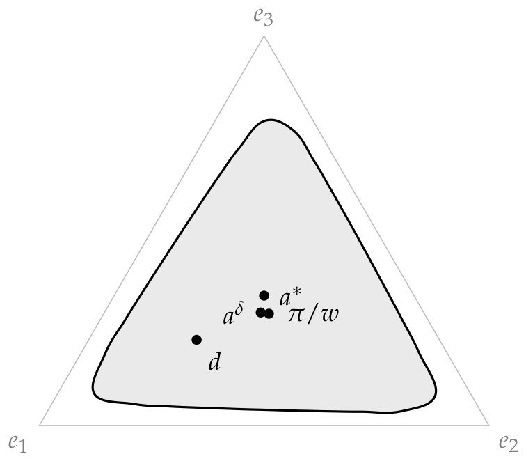
Disclaimer/Publisher’s Note: The statements, opinions and data contained in all publications are solely those of the individual author(s) and contributor(s) and not of MDPI and/or the editor(s). MDPI and/or the editor(s) disclaim responsibility for any injury to people or property resulting from any ideas, methods, instructions or products referred to in the content. |
© 2026 by the authors. Licensee MDPI, Basel, Switzerland. This article is an open access article distributed under the terms and conditions of the Creative Commons Attribution (CC BY) license (http://creativecommons.org/licenses/by/4.0/).
Copyright: This open access article is published under a Creative Commons CC BY 4.0 license, which permit the free download, distribution, and reuse, provided that the author and preprint are cited in any reuse.