

Submitted:
10 August 2026
Posted:
10 August 2026
You are already at the latest version
Abstract
Acoustic logging while drilling (LWD) provides formation shear-wave velocity in real time during drilling, supporting geosteering and geomechanical evaluation. Shear-wave velocity is currently extracted by slowness–time coherence (STC) processing, which relies on a grid search for the global extremum; its hard decision is prone to dense outlier spikes in multi-event wavefields, and its computational burden is unfavorable for downhole real-time evaluation. We propose a lightweight convolutional neural network (CNN) that regresses the inter-receiver moveout directly from array waveforms; five-fold cross-validation on a synthetic dataset yields a median relative velocity error of 2.51% ± 0.16%. The numeric and image-inversion domains, with either a threshold mask or an Attention U-Net segmentation mask, give consistent velocities, with differences between mask methods of ≤0.6%, and 2.5–4.5 kHz band-pass filtering brings the two domains into convergence. As a control, supervised regression labeled by a measured STC log attains per-gather r = 0.72 over the full well interval under random splitting, but r drops to 0.20 under depth-blocked cross-validation that removes near-neighbor leakage, delimiting the applicability boundary of this proxy route. Inference is a single deterministic forward pass, the model occupies only 266 KB, and it runs approximately 25× faster than vectorized STC, making it suitable for edge deployment.
Keywords:
acoustic logging while drilling (LWD)
; convolutional neural network
; moveout regression
; cross-validation
; threshold mask
; edge deployment
1. Introduction
Acoustic logging while drilling (LWD) provides formation elastic-wave velocities in real time during drilling, supporting geosteering, pore-pressure prediction, and geomechanical evaluation without a dedicated wireline run [1,2,3]. A central difficulty of while-drilling measurement and downhole intelligent monitoring is that both the telemetry bandwidth and the downhole computing power are limited in the while-drilling scenario, so processing is best performed locally and in a lightweight manner near the sensor; this practical constraint is the starting point of the method design in this paper [4].
In slow formations, where the formation shear-wave velocity is lower than the acoustic velocity of the borehole fluid, the refracted shear head wave no longer exists, and monopole measurements therefore lose the direct route to the formation shear wave. In this case, one must turn to multipole excitation, which excites a dispersive guided wave in the borehole whose phase velocity at low frequencies approaches the formation shear-wave velocity, from which the shear slowness can be inverted [5,6,7]. For an axially equispaced receiver array, the formation shear information reduces to the constant time shift with which this guided-wave packet advances across the traces, i.e., the time difference between adjacent receivers.
For four decades, the standard method for reading this time shift from array waveforms has been slowness–time coherence (STC) [8,9]: scanning over a slowness–time grid and picking the coherence maximum, with the coherence measure inherited from semblance in multichannel seismic analysis [10]. This paradigm has two prominent limitations in field measurements. First, the hard decision of taking the global maximum: once a secondary coherent arrival captures the peak, the velocity log along depth exhibits dense outliers. Second, the computational cost of the grid search is unfavorable both to high-throughput reprocessing and to real-time downhole evaluation, where telemetry bandwidth is limited and lightweight inference near the sensor is preferred [11,12,13]. Classical improvements have proceeded along two routes, statistical efficiency and dispersion bias: the former improves statistical efficiency and resolution through parametric spectral estimation and maximum-likelihood frameworks [14], whereas the latter removes systematic bias through dispersion correction, such as dispersive STC processing [15] and high-resolution dispersion inversion [16]. Neither, however, departs from the framework of model fitting followed by extremum picking, so the hard-decision outliers and the computational burden persist, leaving room for replacing this paradigm with a learned continuous mapping.
Deep learning has been applied to related problems along three input types—curves, waveforms, and images—and its overall progress in geophysics and seismology is reviewed in [17,18]. Closest to the main line of this paper is the synthetic-training paradigm: supervised training on synthetic forward-modeled data with known ground truth followed by transfer to measured data [19,20,21], together with direct regression of velocity or slowness from array waveforms [22] and physics-informed networks for dispersive dipole data [23,24]. Other applications, including the reconstruction of sonic transit time from other logging curves [25,26], first-arrival picking on waveforms [27,28,29], and the regression of physical quantities from rendered time–frequency or signal images [30,31,32], are more distantly related to the present problem. The main line of this paper belongs to the synthetically supervised category: the network is trained on a synthetic dataset of inter-receiver moveout to learn the kinematic mapping and is then applied to the measured dataset; the measured moveout is a quantity intrinsic to the data and is converted to shear-wave velocity via the effective receiver spacing in Table 1. Unlike explicit dispersion correction or inversion [16,23,24], we do not model dispersion within the network; instead, it is folded into the end-to-end morphological mapping and uniformly absorbed by the value of the effective receiver spacing.
As a comparison, we also examine another supervised route: end-to-end supervised training from scratch directly on the measured dataset, with a measured commercial STC velocity log (hereafter the measured STC) as the label. This route is akin to pseudo-label self-training and functional knowledge distillation, in that its label is itself a self-contained processing-result curve [33,34]; and because the label may contain outliers caused by secondary arrivals capturing the peak, it also bears the character of learning with noisy labels [35]. It yields output on the same scale as the measured STC, which facilitates direct comparison with the measured log, and its attainable accuracy is comparable to that of the measured STC curve. We include it as a comparison to clarify the distinct roles of synthetically supervised shear-wave velocity extraction and a measured-label-supervised proxy.
To our knowledge, there is still no shear-wave velocity estimation model that learns the kinematic mapping of inter-receiver moveout under synthetic supervision, performs extraction on measured data without external labels, supports downhole or near-sensor edge deployment through a single deterministic forward pass, and substantiates its robustness by multiple consistency checks rather than a single reference. To this end, we propose a synthetically supervised lightweight convolutional neural network (CNN) method for inter-receiver moveout regression, which realizes shear-wave velocity extraction through the array-geometry conversion, and we evaluate it on a measured dataset from a quadrupole remote-detection acoustic logging interval of a physical experimental well in a slow formation. The main contributions are as follows:
1. We train a lightweight CNN on a synthetic dataset of inter-receiver moveout to regress the moveout, learning the kinematic mapping from the two-dimensional morphology of the gather to the inter-receiver moveout; when applied to measured data, it requires neither per-depth manual labeling nor any external velocity log. On the synthetic benchmark, the five-fold cross-validation median relative error in velocity is 2.51%, and that on the held-out test set is 2.11%.
2. We present a supervised variant that uses the measured STC log as the label; under random splitting it follows the central trend of the measured STC and markedly reduces the variance, but depth-blocked cross-validation with near-neighbor leakage removed reveals weak cross-depth generalization, thereby delineating the applicability boundary of this proxy route.
3. The model occupies only 266 KB and runs approximately 25 times faster than a vectorized STC grid search on the same hardware; the zero-parameter threshold mask matches the accuracy of an Attention U-Net segmentation-mask front-end with approximately 0.49M parameters, and the entire inference is a single deterministic forward pass, making the method suitable for downhole or near-sensor edge deployment.
The remainder of this paper is organized as follows. Section 2 presents the methodology: we first give an overview of the overall design rationale and processing workflow, then successively lay out the theoretical foundations—quadrupole measurement physics and dispersion, the linear arrival-time model and kinematic identifiability, STC processing, and the statistical limits of moveout estimation—and subsequently describe the acquisition system and measured dataset, the lightweight CNN with the threshold-mask front-end, synthetically supervised training, application to measured data, the measured-STC supervised regression, and the evaluation protocol with statistical tests. Section 3 reports the results, in turn: inter-receiver moveout regression accuracy on the synthetic benchmark, shear-wave velocity extraction on the measured interval, multiple consistency across domains and processing, the comparison and generalization test of the measured-STC label proxy, and computational cost and edge feasibility. Section 4 discusses the mechanistic interpretation, the positioning of the two supervised routes, practical implications, and limitations, and Section 5 concludes.
2. Methods and Principles
We use a synthetically supervised lightweight CNN to regress the inter-receiver moveout directly from array gathers and then convert it to shear-wave velocity through the array geometry. This design exploits the kinematic structure of the quadrupole measurement: in slow formations, the shear-wave information is carried by the quadrupole guided-wave mode, whose low-frequency phase velocity approaches the formation shear-wave velocity [5,6], and the observation of this mode on an axially uniform receiver array reduces to a single kinematic quantity—the constant time shift of the wave packet across traces, i.e., the inter-receiver moveout .
Under the linear arrival-time model, the arrival time is a linear function of the receiver index, and its slope is ; the formation shear-wave velocity is obtained from and the array geometry:
where is the receiver spacing and is the time sampling interval. depends only on the relative phase advance of the wave packet across traces and is independent of both the absolute arrival time and the overall amplitude scale. Standard STC processing performs a grid search over the slowness–time plane and takes the global coherence maximum [8,9]; this hard decision can switch wholesale to a secondary arrival in the wavefield, which appears as dense outlier spikes on the velocity curve along depth.
STC processing is the baseline for shear-wave velocity extraction, and understanding its decision mechanism is a prerequisite for understanding the motivation of our method. Figure 1 illustrates this processing with an example quadrupole array record: (a) shows the 12-trace array waveforms, in which the borehole mud/collar wave, the target quadrupole shear arrival, and the Stoneley wave arrive in succession; the target wave packet of interest advances linearly across the trace index with a constant time shift, the slope of the dashed line corresponds to the slowness, and the shaded band marks its time window; (b) shows the coherence distribution over the slowness–time plane, where several arrivals each form a coherence peak and the slowness at the global maximum is the STC estimate. At the level of results, the figure shows that the STC output is taken from the global maximum of a multi-peak coherence surface. Further analysis reveals that its instability is structural: semblance-type coherence measures are near-optimal under the premise of a single coherent arrival, whereas measured LWD wavefields often contain coexisting secondary coherent arrivals such as reflections from adjacent wells, collar waves, and coda, so the coherence surface is multi-peaked; when a secondary peak approaches the target peak, the hard decision can switch wholesale between peaks. This is precisely the root cause of the dense outlier spikes on the velocity curve along depth, and it is the direct motivation for replacing the scan-and-pick-the-extremum paradigm with continuous regression in this work.
Accordingly, the network is trained on a synthetic forward-modeled dataset with known injected inter-receiver moveouts [19,20,21] and regresses the moveout from threshold-masked gathers; no per-depth labels or reference velocity curves are required on the measured side. The regressed moveout is determined by the waveforms themselves and is converted to shear-wave velocity through Equation (1) using the effective receiver spacing in Table 1.
Figure 2 overviews the overall processing pipeline from array gathers to shear-wave velocity, organized around direct regression of the kinematic quantity. Along the main path, the measured 12-trace waveforms and their gather image (12 × 400) are DC-removed and normalized, after which a threshold mask retains the high-amplitude coherent wave packet and zeroes the remaining samples; the masked gather is fed into the lightweight CNN, which regresses the inter-receiver moveout in a single deterministic forward pass, and the shear-wave velocity is then output via the conversion in Equation (1). The training branch is supervised by a synthetic forward-modeled dataset with known injected moveouts, so no per-depth labels are needed on the measured side. The rationale for this design lies in identifiability: what the array data can uniquely identify is the relative phase advance of the wave packet across traces, and the conversion from moveout to absolute velocity requires only one additional geometric parameter, the receiver spacing, so the network concentrates on learning a quantity intrinsic to the data.
2.1. Theoretical Foundations
2.1.1. Quadrupole Measurement
In slow formations, the formation shear-wave velocity is lower than the acoustic velocity of the borehole fluid, the critical refraction condition is no longer satisfied at the borehole wall, and the refracted shear head wave gliding along the wall therefore does not exist; monopole direct arrivals thus cannot directly provide formation shear-wave information. Multipole excitation must then be employed, of which the quadrupole is the most typical: rather than a body-wave head wave, a quadrupole source in a fluid-filled borehole excites a dispersive guided-wave mode propagating along the borehole axis, whose phase velocity varies with frequency and approaches the formation shear-wave velocity at low frequencies, so the formation shear slowness can be inverted from the low-frequency phase velocity of this mode [5,6]; see [7] for the multipole-source theory of borehole multipole acoustic measurements and [36] for a systematic treatment of borehole acoustic guided waves.
Formally, the formation quadrupole mode is given by the branch of the period equation for a fluid-filled borehole. Denote the dispersion relation of this branch as
where is the axial wavenumber and is the angular frequency; , , and are the formation shear-wave velocity, compressional-wave velocity, and density; and are the acoustic velocity and density of the borehole fluid; and is the borehole radius. For a given frequency, the root satisfying Equation (2) determines the phase velocity of this mode [5,7,36]. The branch has a cutoff frequency and propagates only for ; as , the phase velocity approaches the formation shear-wave velocity from below, and it falls progressively lower as frequency increases [5,6,36].
The mode is inherently dispersive, which has direct consequences for processing: converting a single moveout to velocity under a nondispersive assumption systematically underestimates the shear-wave velocity and overestimates the slowness, because the phase velocity approaches from below only at the low-frequency end of the branch and lies lower at higher frequencies; for the dispersion-induced slowness bias and the rejection of spurious modes, see dispersive STC processing [15] and high-resolution dispersion inversion [16]. In this work, dispersion is not modeled explicitly in the network; instead, it is folded into the end-to-end morphological mapping and absorbed collectively through the choice of the effective receiver spacing.
The LWD environment introduces an additional source of interference: the steel drill collar itself constitutes an acoustic waveguide that supports a quadrupole mode and can contaminate the formation mode. This is precisely one of the important reasons for choosing the quadrupole. Within the low-frequency band of interest, i.e., below the cutoff frequency of the collar quadrupole mode, the collar quadrupole mode does not propagate and is effectively suppressed, and the formation quadrupole mode is relatively dominant, which favors separating and extracting the formation shear wave with little interference from the collar wave [5,6].
At the level of array reception, the physics above reduces to a simple kinematic fact: the wave packet of interest arrives at the axially uniformly spaced receivers in succession with a constant time shift, and this constant time shift is the inter-receiver moveout. The next section formalizes this.
2.1.2. Linear Arrival-Time Model
Let the measured guided-wave mode advance along the borehole axis with slowness , and let denote the axial coordinate of the -th receiver (); the arrival time on that receiver then satisfies
The arrival time is a linear function of trace index: the intercept is determined by the excitation time and the propagation path from the source to the first receiver, whereas the slope is determined by the apparent slowness of the measured guided-wave mode, which approaches the formation shear slowness at the low-frequency end. For an equally spaced array, the arrival-time increment between adjacent receivers is constant, where is the receiver spacing; expressed in samples, this increment is the inter-receiver moveout , with the sampling interval. The velocity conversion (Equation (1)) is nothing more than the inverse of this linear arrival-time model: the same guided-wave mode advances linearly across the equally spaced receivers at a single apparent velocity, and the slope of its time shift across the array uniquely encodes the measured slowness.
Two points follow. First, is a purely kinematic quantity: it depends only on the relative phase advance of the wave packet across receivers and is independent of the absolute arrival time and of any overall amplitude scale, and it is therefore intrinsic to the data. Second, the identifiability of velocity is equivalent to the identifiability of the cross-receiver phase slope: the problem of shear-wave velocity extraction thereby reduces to the robust estimation of a constant inter-receiver time shift. This estimation primitive is shared by classical processing and by the learning-based method of this paper, and it also provides the physical basis for the invariance design of the network (insensitive to global time shifts and amplitude scaling, sensitive to cross-receiver phase).
This model also provides the estimation-theoretic basis for our method design. In shear-wave velocity extraction, what the data can uniquely identify is the kinematic invariant, namely the inter-receiver moveout ; the conversion from to the absolute velocity must introduce the receiver spacing through Equation (1), and the latter constitutes an overall scale degree of freedom that cannot be determined internally from the cross-receiver phase. Accordingly, we assign the identifiable kinematic invariant to a data-driven, geometry-independent continuous estimator, while the receiver spacing required for velocity conversion is supplied as a single geometric parameter given in Table 1. This treatment explicitly separates the quantities that the cross-receiver phase can determine directly from those that must be introduced through the conversion.
2.1.3. Slowness–Time Coherence
For four decades, the standard method for extracting this time shift from array waveforms has been STC processing [8,9], whose coherence measure, semblance, originates from coherence measures in multichannel seismic data analysis [10]. It is constructed as follows: on the slowness–time plane spanned by the candidate slowness and the window start time, the traces are moveout-corrected, aligned, and stacked according to the time shift implied by each candidate slowness, and the coherence is then computed within a fixed time window as the ratio of the energy of the aligned stack to times the sum of the individual trace energies, where is the number of receivers. Denoting the waveform of the -th receiver by and its axial coordinate by (), for candidate slowness and window start time ,
Here the window starts at and contains a fixed number of samples; the factor of in the denominator ensures and makes the measure invariant to an amplitude scale common to all traces. The candidate slowness and the inter-receiver moveout are in one-to-one correspondence through . STC takes as its estimate the slowness (equivalently, the moveout) corresponding to the global maximum of over the plane, which is then converted to velocity via Equation (1) (Figure 1). The scale invariance of semblance removes only the amplitude scale common to all traces; inter-trace gain differences still degrade the constructive alignment of the stack and must therefore be leveled by per-trace amplitude normalization in preprocessing.
From an estimation-theoretic viewpoint, measures the fraction of the total energy captured by the aligned stack: when all traces are perfectly coherent under the candidate time shift, and its expectation is approximately for purely incoherent noise. For the idealized model of a single nondispersive arrival in additive white Gaussian noise, and under the condition that the total in-window energy is approximately invariant to the candidate slowness, maximizing semblance is nearly equivalent to maximum-likelihood slowness estimation; this is the theoretical basis for the near-optimality of STC [8]. The route that improves the statistical efficiency and resolution of slowness estimation through parametric spectral estimation and maximum-likelihood frameworks is presented in [14].
This near-optimality, however, presupposes a unique coherent target. Measured LWD wavefields often contain several secondary coherent arrivals, such as reflections from nearby structures or adjacent wells, strong collar and tool waves, and formation coda; in such a multi-event wavefield, becomes multimodal, and the global maximum is essentially a winner-take-all hard decision: the estimate depends only on which peak of the coherence map is highest, regardless of its physical origin. The argmax operator is inherently discontinuous with respect to data perturbations. When two peaks are close in height, a small perturbation of the wavefield can switch the global maximum between them, and the estimate jumps wholesale to the slowness of the other event rather than degrading continuously; once any secondary event forms a coherence peak at an erroneous slowness that is comparable to or even higher than that of the target wave packet, the decision jumps abruptly to that erroneous event, manifesting as dense, large-amplitude outlier spikes along the depth-wise velocity log. Such large outliers are therefore not random measurement noise but a structural product of a hard-decision coherence measure under multi-event competition; multi-peak extraction, slowness tracking, and quality control in production-grade STC workflows can mitigate, but cannot fully eliminate, this decision switching. Compounding this, the dispersion of the quadrupole mode causes the coherence-peak position to drift with the spectral energy distribution, introducing slowness bias or allowing spurious modes to capture the peak [15,16]; the computational cost of the slowness–time grid search also rises markedly with resolution, which is unfavorable for downhole real-time evaluation. Classical improvements along the statistical-efficiency [14] and dispersion-correction [15,16] routes retain grid scanning or model fitting as their computational core, and the decision still reduces to taking an extremum on a coherence or likelihood surface, so neither the structural outliers under multi-event competition nor the computational burden is fundamentally removed. In this paper, we replace this hard decision and grid search with a continuous mapping determined by the wave-packet morphology.
2.1.4. Moveout Estimation
The precision with which the inter-receiver moveout can be read out is subject to a statistical limit that is independent of the specific estimator and is jointly determined by the waveform energy, the bandwidth, and the array geometry. For the model of a single arrival of known waveform in additive white Gaussian noise (one-sided power spectral density ), the Cramér–Rao lower bound for an unbiased moveout estimate is
where is the signal energy and is the root-mean-square angular bandwidth of the signal (the square root of the second moment of angular frequency weighted by the signal energy spectrum) [37]; the corresponding bound for the passive two-channel stochastic-signal case is given in [38]. This bound constrains unbiased moveout estimators; when the waveform is unknown the bound can only be larger, so Equation (5) remains a valid lower bound, whereas a biased regression mapping trades bias for variance and is not directly constrained by it. Parametric spectral-estimation processing aimed at statistical efficiency [14] uses precisely such limits as its benchmark, connecting to the semblance near-optimality argument of the preceding subsection. Equation (5) shows that the attainable precision of the moveout tightens as the signal-to-noise ratio and the effective bandwidth increase: the quadrupole wave packet is a band-limited signal, so the readout precision of a single-pair inter-receiver moveout is limited, but there is no obstacle in principle.
Array redundancy further tightens the estimation of the moveout slope. Under the linear arrival-time model, if the arrival-time readings of equally spaced receivers each contain independent errors of variance , then for a least-squares fit of the straight line of arrival time versus trace index, the variance of the slope (slowness) estimate scales as
[39]: at a given spacing, the variance decreases approximately with the cube of the number of receivers; at a given number of receivers, it tightens with the square of the array aperture. In other words, even though the readout precision of a single-pair inter-receiver moveout is limited by Equation (5), the linear redundancy across the array still allows the moveout to be identified with high precision. This provides statistical support for the moveout-regression design described above: under the kinematic model of a single dominant arrival, cross-array redundancy makes the moveout information ample and robustly readable; in multi-event situations, discriminating the target mode additionally requires a prior on wave-packet morphology, which we inject through synthetic supervision. Combined with the multi-peak competition analysis of Section 2.1.3, the structural outliers of STC should be attributed to its decision mechanism rather than to an information deficit in the single-arrival sense, and this provides the statistical feasibility basis for estimating the moveout with a continuous mapping.
2.2. Data and Extraction Method
2.2.1. Measured Dataset
The measured data used in this study were acquired by a quadrupole-array acoustic logging-while-drilling (LWD) tool. The receiver section comprises an axial array of receivers with a receiver spacing of m and a time sampling interval of µs; the source–receiver offset of m defines the axial geometry of the array but does not enter the array velocity conversion of Equation (1), which is determined by the inter-receiver moveout. The first samples of each record were retained, which already contain the complete arrival of the wave packet of interest. The acquisition and processing constants are summarized in Table 1.
Reproducibility of the method requires a single source for all acquisition and processing constants. Table 1 summarizes these constants: the number of receiver channels and the time sampling interval define the acquisition geometry; the effective receiver spacing enters the velocity conversion of Equation (1); and the threshold-mask parameter and the band-pass frequency band specify the fixed settings of the processing chain. The symbols and values in all equations in the text follow this table. Consequently, the entire workflow contains no free parameters that must be tuned for each well interval, and the configuration burden is minimal.
The measured data were acquired in the remote-detection acoustic logging experiment [40] at the National Key Laboratory of Deep Oil and Gas, China University of Petroleum (East China), from the laboratory's physical experimental well; they are actual measurements on a physical well rather than numerical simulations. The target formation is a slow formation: the formation shear-wave velocity is lower than the acoustic velocity of the borehole fluid, the critical refraction condition is not satisfied at the borehole wall, and no refracted shear head wave exists, so quadrupole excitation is required; what this paper extracts is precisely the formation shear-wave velocity given by the quadrupole guided-wave mode.
The dataset for this well interval is available in two forms. The first is the raw numeric waveforms sampled directly by the tool, hereafter the numeric domain; the second is rendered waveform images, hereafter the image-inversion domain, the latter reflecting the reality that legacy and exchanged data are often archived as rendered plots. The main-line extraction is performed in the numeric domain, which is free of rendering distortion and is the cleanest; the image-inversion domain is used for cross-domain consistency checks. Quantitative amplitudes in the image-inversion domain are recovered by self-calibrated inversion from the color bar embedded in each PNG: the colormap is sampled from a fixed pixel band in the figure to build a color-to-amplitude lookup table from +1 to −1; the in-axes region is cropped according to the fixed layout and divided into a 12 × 400 cell grid; and the median RGB of each cell is inverted to amplitude by nearest-neighbor lookup in the LUT, with near-gray cells set to zero.
In both domains, each gather is preprocessed by first removing the per-trace DC component and then normalizing to unit maximum absolute amplitude. DC removal also levels inter-trace gain differences, which benefits the aligned stacking underlying the coherence measure.
No independent per-depth ground truth from core or wireline logging is available for this well interval. The main-line network is not supervised by any external curve. The separately configured measured-STC supervised-regression comparison variant uses a measured STC shear-wave velocity log with 1032 depths, with a median of 1095 m/s, an interquartile range (IQR) of 190 m/s, and a range of 826–1544 m/s, paired one-to-one by depth with the image-inversion-domain gathers.
2.2.2. Lightweight CNN
The estimator takes the threshold-masked gather as input and regresses the inter-receiver moveout end to end. Let denote the 12 × 400 gather normalized per gather to unit maximum absolute amplitude; the network input is the threshold-masked (), i.e., samples whose normalized amplitude is not below the threshold are retained element-wise and all others are set to zero, where is the indicator function. is processed by a convolutional network deliberately designed to be small, so as to reduce the parameter count and compute and to facilitate a single deterministic lightweight inference at the downhole or near-sensor edge [11,12,13]. The network contains four convolutional blocks, followed by global average pooling, a 64-unit fully connected layer with ReLU, and a single linear output unit that predicts the moveout magnitude , which is then converted to velocity via Equation (1). The network has approximately 68,000 trainable parameters. The convolution kernels and pooling are anisotropic along the two axes: finer along the channel axis of only 12 traces than along the 400-point time axis, thereby preserving the inter-trace phase information that carries the moveout while aggregating substantially along the time axis; the moveout encoded by this cross-trace phase is exactly the quantity on which the velocity conversion via Equation (1) relies.
Figure 3 shows the architecture of the regression CNN: the input is the threshold-masked 12 × 400 gather, which passes through a series of anisotropic convolutional blocks that extract the two-dimensional morphological features of the wave packet along the channel and time axes; after compression by global average pooling, a fully connected layer outputs the scalar inter-receiver moveout. The architecture contains no search stage over any particular slowness grid; the forward pass is the estimate. In terms of inductive bias, the anisotropic convolution kernels match the constant phase slope of the wave packet along the channel axis; the translation equivariance of convolution renders the estimate insensitive to a global time shift of the arrival; per-gather normalization and masking endow it with invariance to amplitude scaling, of the same origin as the scale invariance of semblance; and the fact that the output is a continuous quantity, with no decision mechanism that switches between peaks, is the structural reason its velocity log is smooth along depth.
Table 2 lists the operators, kernel sizes, and output dimensions of the network layer by layer; its significance lies in quantifying what "lightweight" means: the entire model is only 266 KB, far smaller than the Attention U-Net segmentation front-end with approximately 0.49M parameters. The task only requires regressing a single kinematic scalar from two-dimensional morphology, and wave-packet gating has already been accomplished by the zero-parameter mask; the fact that the network matches the accuracy of the Attention U-Net front-end indicates that the task does not call for a high-capacity model, and the lightweight design does not come at the cost of accuracy. The model size bears directly on the deployment form: at this scale of parameter count and storage, the network fits into downhole or near-sensor edge computing environments and completes inference with a single deterministic forward pass, which forms the basis of the computational cost measurements.
The threshold mask operates as follows. After per-gather normalization, high amplitudes concentrate in the coherent wave packet that carries the inter-receiver moveout, i.e., the event advancing across traces with a constant slope, whereas low-amplitude samples are mostly occupied by incoherent background, weak residual tool and collar waves, and image-inversion residuals. The threshold mask accordingly applies a single hard amplitude gate: it retains the high-amplitude, moveout-bearing structure and zeroes out sub-threshold low-amplitude interference wholesale, so that the subsequent convolutional layers focus on the cross-trace phase structure with less distraction from low-amplitude clutter. This gate is a zero-parameter front-end that introduces no trainable weights and incurs negligible inference overhead. The threshold is taken at the midpoint of the normalized amplitude, balancing retention of the main wave packet against rejection of low-amplitude clutter.
The network implements a deterministic function determined by the parameters , mapping the threshold-masked gather to the moveout-magnitude estimate . Given paired samples , the parameters are fitted with the mean squared error (MSE) in the moveout domain as the objective:
Under this objective, the optimal regression function converges to the conditional expectation , i.e., the expectation of the inter-receiver moveout given the entire gather . The inductive bias is as follows: the moveout manifests as a constant phase slope of the wave packet along the channel axis, the anisotropic convolution kernels extract this cross-trace phase structure layer by layer, and global average pooling then aggregates it into the single scalar . What the network learns is precisely the repeatable mapping from the two-dimensional morphology of the gather to the inter-receiver moveout.
This design also encodes the kinematic invariances explicitly into the estimator. Per-gather normalization and the threshold mask make insensitive to the overall amplitude scale, of the same origin as the scale invariance of semblance; after aggregation by global average pooling, the translation equivariance of convolution [41] renders the output approximately invariant to a global time shift of the wave packet, corresponding exactly to the fact that does not depend on the absolute arrival time . The estimate is therefore driven mainly by the relative cross-trace phase structure.
The essential difference from STC lies in the decision mechanism. The STC estimate is taken from the global maximum of a multi-peaked coherence surface, and when two peaks compete, the decision can switch wholesale between them; in the present method, after the fixed mask front-end, a continuous mapping composed of convolutions, ReLUs, and pooling aggregates the evidence of the entire input into a single estimate—there is no operator that selects "which peak is highest," and hence no corresponding decision-switching mechanism. This structural difference does not by itself guarantee robustness under arbitrary perturbations; its practical effect is corroborated by the observation that the measured extraction exhibits no dense outlier spikes. The main line fits this mapping on synthetic data, whereas the comparison variant fits it on measured STC labels.
2.2.3. Synthetically Supervised Training
The main-line network was supervised on a synthetic forward-modeled dataset, learning the kinematic mapping from the two-dimensional wave-packet morphology to the inter-receiver moveout; no external velocity curve is required when it is applied to measured data [19,20,21]. The synthetic dataset injects a known constant inter-receiver moveout along the channel axis using multi-cycle Gabor wavelets, superimposes interfering reflection events and band-limited random noise, and is calibrated against the measured spectrum so that its frequency band and waveform morphology closely match the measured data. Formally, the synthetic waveform of the -th trace can be written as , where is the multi-cycle Gabor wavelet matched to the measured spectrum, denotes the interference terms crossing the array obliquely at different apparent slownesses, and is band-limited random noise; for each sample, the onset arrival time , the moveout , the interference geometry, and the noise realization are drawn at random.
The regression target is invariant to , to the overall amplitude scale, and to the noise realization; randomizing these nuisance factors during training encourages the network to rely primarily on the invariant feature of the across-trace phase slope to perform the regression. This is precisely the mechanism by which domain randomization enables synthetic-to-measured transfer [42], and its cross-domain effectiveness is corroborated by the consistency checks.
The ground-truth moveout of each sample is injected via ; the synthetic geometry adopts m, consistent with the receiver spacing, so that the synthetic velocities are of slow-formation magnitude and the injected inter-receiver moveouts therefore fall within the measured range. What the network learns is the across-trace wave-packet slope itself, scaled to velocity only through , so the mapping learned from synthetic training transfers directly to measured data.
Training used exactly the same network and preprocessing as the main line and was performed from scratch with a moveout-domain MSE loss: a 4000/800/800 training/validation/test split, the Adam optimizer, an initial learning rate of 0.001 halved every 12 epochs, 40 epochs in total, a batch size of 64, and L2 regularization of 0.001. Training and all timing experiments were carried out in MATLAB R2026a on a single NVIDIA RTX 5080 GPU, and a single training run completed within a few minutes.
2.2.4. Application to Measured Data
The trained network was applied to the measured numeric-domain dataset: after DC removal, normalization, and threshold masking , each gather was processed by a single deterministic forward pass to regress the inter-receiver moveout magnitude , which was then converted to shear-wave velocity via Equation (1). The measured moveout is a quantity intrinsic to the data and is independent of any subsequent geometric assumptions.
Converting the moveout to absolute velocity via Equation (1) additionally requires the receiver spacing . The receiver spacing = 0.1 m from Table 1 was used for this conversion; this effective spacing is an equivalent geometric parameter that absorbs systematic effects such as dispersion and the processing chain. It determines only the overall scale of the absolute velocity and does not alter the relative shape, vertical variation, or scatter of the velocity log.
We emphasize that the measured inter-receiver moveout is intrinsic to the data and that the choice of receiver spacing affects only the absolute velocity scale; the source–receiver offset merely defines the axial geometry of the array and does not enter the array velocity conversion of Equation (1).
2.3. Comparison Protocols
2.3.1. Measured-STC Supervision
For comparison, we implemented a supervised regression variant that uses the measured STC shear-wave velocity log as its label [33,34], which belongs to the same family as prior work in well logging that generates labels from deterministic relations to supervise acoustic-log prediction [34]. On the image-inversion-domain dataset, this variant trains a CNN with the same architecture as the main line end to end from scratch, with a measured STC shear-wave velocity log as the supervision target. The measured STC velocity is converted to the regression target by
appears consistently in both the label encoding and the velocity decoding and therefore cancels, so the converted velocity is independent of the specific value of ; the network outputs velocities on the scale of the measured STC labels.
Preprocessing is identical to the main line. The data were split 80/20 into training and validation subsets; the validation subset does not update the weights and is used only to select the best epoch by validation loss, while the labels of the training subset undergo label-preserving augmentation.
From a learning-theory perspective, training with the MSE loss of Equation (7) on noisy labels drives the regression function toward the conditional expectation, where is the latent ground truth and is the label error. For isolated spikes in the labels caused by secondary arrivals capturing the coherence peak, the arrival evidence may indeed remain in the input , but such samples constitute a minority of the training set and their morphology–velocity correspondence contradicts that of the majority: under the conditional averaging of MSE, the few contradictory labels are diluted by the majority-consistent mapping, and the network tends to output the estimate determined by the majority of samples rather than reproduce the spikes. On the other hand, when the information contained in the input is insufficient to fully determine the label, the spread of the conditional expectation is necessarily smaller than that of the labels, and the predictions shrink toward the label mean. This shrinkage can be formalized by the law of total variance [39]:
By Equation (9), the variance of the ideal regression solution satisfies , and the difference between the two is exactly the conditional variance of the labels that the input cannot explain; the more limited the explanatory power of the input for the labels, the more pronounced the shrinkage.
2.3.2. Evaluation Protocol
Synthetic evaluation reports, on the test set, the mean absolute error (MAE) of the moveout, the median relative error of the velocity converted from the moveout, and the fractions of samples within 5%/10%, with stability assessed by five-fold cross-validation. Measured extraction reports the median and interquartile range (IQR) of the shear-wave velocity and the curve along depth.
Cross-domain consistency is tested at the same effective receiver spacing: the extracted velocity medians and the per-image mask intersection over union (IoU) are compared between the numeric domain and the image-inversion domain, between the threshold mask and the Attention U-Net segmentation mask, across different band-pass filters, and for the quadrupole combination, quantifying the robustness of the extraction to processing details; the results are further cross-checked against self-computed STC on the same dataset.
For the measured-STC supervised regression, we report, on the held-out validation subset, the median ratio to the measured STC, the per-gather median relative error, the fractions within 5%/10%, and the correlation coefficient , compared against a constant baseline given by the median of the training-set labels; over the full well interval, we report the median ratio, IQR and standard deviation. Variance differences are tested in two ways: first, paired bootstrap interval estimation, resampling gathers with replacement times and taking the 2.5/97.5 percentiles to construct confidence intervals; second, the Brown–Forsythe test, which is robust to heavy tails. Cross-depth generalization is tested by depth-blocked five-fold cross-validation that removes near-neighbor leakage, with each fold holding out a contiguous well interval.
Runtimes were measured on the complete dataset: the CNN uses GPU batch processing, and the reference is a vectorized STC grid search parallelized over 16 cores on the same hardware, with a slowness–time grid spanning velocities of 1000–3500 m/s at a step of 25 m/s and a time window of 45 samples. Timing was performed on the same 1032 gathers with repetitions, measured after warm-up and reported as mean ± standard deviation, to quantify the speedup obtained by replacing the grid search with a single deterministic forward pass.
3. Results
3.1. Inter-Receiver Moveout Regression Accuracy
On the synthetic benchmark with known ground truth, the network regresses the inter-receiver moveout approximately without bias, with a median relative error of about 2%–2.5%. The synthetic dataset was calibrated against the measured data, with its frequency band and waveform morphology close to the measurements; its construction and comparison with the measured data are shown in Figure 4.
The synthetically supervised route is valid only if the synthetic training dataset and the measured dataset are sufficiently close along the feature dimensions on which the network relies. Figure 4 provides a visual check: the top row shows examples of measured gathers, in which the target wave packet advances linearly across the trace index with superimposed background disturbances; the lower three rows show examples of synthetic gathers, in which a known constant inter-receiver moveout is injected along the channel axis using multi-cycle Gabor wavelets, interfering events and band-limited random noise are superimposed, and the dominant frequency and signal-to-noise ratio are calibrated against the measurements. The results show that the two groups are close in frequency band, wave-packet extent, and linear cross-trace advance. The underlying mechanism is domain randomization: the regression target depends only on the cross-trace phase slope, and randomizing moveout-irrelevant factors on the synthetic side—waveform details, amplitude, and noise realizations—drives the network to rely on this invariant feature for regression. Transfer therefore does not require pixel-wise similarity between synthetic and measured data, only that the two share the same kinematic invariant and its morphological carrier.
The accuracy on the synthetic benchmark can serve as a benchmark only after the contingency of a lucky split has been ruled out. Figure 5 presents the per-fold results of five-fold cross-validation for the synthetically supervised regression: (a) shows the median relative velocity error for each fold, fluctuating slightly around the five-fold mean of 2.51% ± 0.16%; (b) shows the fraction of samples with error ≤5% and ≤10% for each fold, stable around 77.3% ± 2.9% and 94.7% ± 0.5%, respectively. The cross-fold dispersion is only a few tenths of a percent, indicating that the accuracy is insensitive to the data split. In terms of evaluation design, cross-validation and the held-out test have clearly distinct roles: the former demonstrates the stability of the accuracy, whereas the latter provides an unbiased point estimate on independent samples, and only when the two corroborate each other do they constitute a complete benchmark.
With stability confirmed by cross-validation, the held-out test set provides point estimates and the error structure on independent samples. Figure 6 evaluates this test from three complementary perspectives: (a) a scatter plot of predicted versus true velocity, with samples tightly clustered along the 1:1 line and the ±5%/±10% reference bands covering the vast majority of samples; (b) a histogram of the signed relative error, approximately normal in distribution with a median bias of only +0.63%; (c) the cumulative distribution of the relative error, with 83.0%, 96.5%, and 98.9% of samples within 5%, 10%, and 15%, respectively, and a P95 of 9.0%. Regarding what this error structure implies, the near-zero bias indicates that the network introduces no systematic over- or underestimation, the errors being mainly small random fluctuations around the true values; the controlled tails mean that, along the depth curve, the errors manifest as a dispersion describable by robust statistics such as the median and interquartile range (IQR), rather than as trend-like drifts or frequent gross errors.
Table 3 summarizes the same held-out test with quantitative metrics, providing point estimates that can be directly cited and compared: R² = 0.947, r = 0.974, CCC = 0.973, RMSE of 51 m/s, MAE of 35 m/s, a median relative velocity error of 2.11%, and a gross-error fraction (relative error > 20%) of only 0.50%. The correlation-type and error-type metrics corroborate each other; the held-out point estimate of 2.11% is close to the five-fold cross-validation result of 2.51% ± 0.16%, further indicating that the benchmark accuracy is not the product of a particular split but the stable performance of the network on this synthetic distribution.
3.2. Shear-Wave Velocity Extraction
The synthetically trained network extracts the shear-wave velocity depth by depth on the measured well interval without retraining; the resulting curve is stable along depth, with none of the STC-style dense outlier spikes. Over 2198 consecutive depths in the numeric domain, the extracted velocity has a median of 1200 m/s and an IQR of 72 m/s, and the inter-receiver moveout has a median of 3.02 samples/channel.
Over 2000 consecutive depths in the image-inversion domain, the inputs are waveform pixel images, the same effective receiver spacing as in the numeric domain is used, and no domain-specific retuning is performed: the extracted velocity has a median of 1053 m/s and an IQR of 118 m/s; has a median of 3.44 samples/channel with a unimodal, concentrated distribution, corresponding to an inter-receiver moveout of about 69 µs. The central trend of the velocity log along depth is stable.
The measured extraction is the final output stage of the method: the synthetically trained network is applied directly to the measured well interval without retraining and without any measured labels. Figure 7: (a,b) an example gather, showing the waveform pixel image and the network input after threshold masking, where the high-amplitude coherent wave packet retained by the mask is the morphology on which the regression relies; (c) the shear-wave velocity log along depth (median 1053 m/s), with a stable central trend and no STC-style dense outlier spikes; (d,e) histograms of the inter-receiver moveout and the shear-wave velocity, respectively, giving the distributions over the whole interval; (f) the hyperbolic velocity–moveout conversion relation, with the domain-wide medians falling on the curve, so that the velocity output and the moveout regression are self-consistent through Equation (1). Regarding the difference from STC, the improvement lies not in a general increase in point-wise accuracy but in the elimination of the dense outliers caused by decision switching—the continuous mapping yields, independently for each gather, a moveout determined by the wave-packet morphology, with no cliff-like jumps caused by a secondary peak overtaking the global maximum on the coherence surface; this is a benefit conferred by the structure of the estimator.
The central trends in both domains are stable along depth; the point-wise dispersion in the image-inversion domain is wider than in the numeric domain, but it likewise shows none of the STC-style dense outlier spikes. This behavior is consistent with the absence of any decision-switching mechanism in the continuous mapping.
3.3. Cross-Domain Consistency
Four mutually independent processing paths yield mutually consistent shear-wave velocities under the same effective receiver spacing, indicating that the extracted inter-receiver moveout is an intrinsic, well-defined quantity of the data. First, acquisition-domain consistency: the numeric-domain extraction has a median of 1200 m/s, whereas the image-inversion domain has a lower median because rendering steepens the cross-trace slope; after a 2.5–4.5 kHz band-pass removes the frequency band in which the two domains differ most, the two acquisition domains converge to the same value, i.e., the inter-domain systematic difference is introduced mainly by rendering and out-of-band components and is eliminated by band-pass filtering. Second, mask-method consistency: replacing the zero-parameter threshold mask with an Attention U-Net segmentation mask of approximately 0.49M parameters gives a per-image mask IoU ≈ 0.97 and a difference in median extracted velocity of ≤ 0.6%. Third, combination consistency: the quadrupole-combination extraction agrees with single components. Fourth, mutual corroboration with self-computed STC: self-computed STC on the same dataset gives a similar median (1052 m/s). On image-inversion-domain gathers, the per-example apparent-velocity line from the CNN regression closely tracks the high-amplitude coherent event advancing linearly across traces.
Figure 8 juxtaposes, as violin plots, the shear-wave velocity distributions of nine CNN extraction variants under the same effective receiver spacing, covering three classes of controls: the numeric domain versus the image-inversion domain (each before and after the 2.5–4.5 kHz band-pass), the zero-parameter threshold mask versus the Attention U-Net segmentation mask, and the quadrupole combination versus single components; the median is annotated above each violin, and the scatter shows all data points. The results show that the medians of the variants are close to one another and that, after band-pass filtering, the two acquisition domains converge to the same value. Two points follow from this analysis. First, the inter-domain systematic difference is introduced mainly by rendering and out-of-band components and can be removed by band-pass filtering; it is thus an explainable, correctable processing-chain effect. Second, all variants share the same effective receiver spacing, so these checks demonstrate the robustness of the extraction to processing details; corroboration of the absolute scale must instead come from the comparison with the independent measured STC.
Figure 9 provides the comparison: when the Attention U-Net segmentation mask replaces the threshold mask, the high-amplitude coherent regions retained from the same gather by the two front-ends overlap almost completely (IoU ≈ 0.97), and the difference in median extracted velocity is likewise ≤ 0.6%. The results indicate that the specific form of the mask is not critical. This equivalence admits a two-level interpretation. In terms of information, what the network relies on is chiefly the two-dimensional morphology of the high-amplitude coherent wave packet itself rather than the fine shape of the mask boundary, so a more elaborate front-end has no room to add value. In engineering terms, a fixed threshold keeps the front-end free of any trainable weights, so the entire inference chain remains a zero-configuration deterministic forward pass—of particular importance for the reliability of downhole deployment.
Figure 10 shows extraction examples on image-inversion-domain gathers: the sloped line overlaid on the waveform pixel image corresponds to the apparent velocity implied by the CNN-regressed inter-receiver moveout, and it closely tracks the high-amplitude coherent event advancing linearly across traces. This per-example correspondence is to statistical consistency what mechanistic evidence is to numerical agreement: it directly shows that the estimate is anchored to coherent structure genuinely present in the data, and that what the network has learned is indeed the kinematic feature of the wave packet's cross-trace moveout slope rather than some shortcut cue incidentally correlated with velocity.
As regards the formation shear-wave velocity itself, the image-inversion-domain extraction median (1053 m/s) and the measured STC median (1095 m/s) differ by less than 5% despite their different scale origins, providing limited mutual corroboration of a formation shear-wave velocity on the order of approximately 1100 m/s for this well interval.
3.4. Comparison Tests Against the Measured STC
Under random splitting, the supervised proxy trained with the measured STC curve as labels follows the central trend of that curve and compresses its global spread. On the held-out validation subset, its median ratio to the measured STC is 1.008, the per-gather median relative error is 7.22%, the fractions within 5%/10% are 34%/65%, and the correlation is r = 0.53, outperforming a constant baseline set to the median of the training-set labels. Over the full well interval, it follows the central trend of the measured STC, and the global spread of its velocities is significantly smaller than that of the measured STC: the standard-deviation ratio is 0.74, the interquartile-range ratio is 0.85, and the Brown–Forsythe test gives p = 1.9×10⁻¹⁴.
Figure 11 directly compares it with the measured STC curve: (a) the superposition of the two velocity curves over the full well interval, with the variant following the central trend of the measured STC; (b) a zoom-in on the most informative well interval, where the variant passes smoothly through the large fluctuations of the labels without tracking them point by point; (c) the velocity distributions of the two, with close medians but a markedly narrower global spread for the variant (standard-deviation ratio 0.74, interquartile-range ratio 0.85). This behavior is consistent with the theoretical expectation that MSE regression converges to the conditional expectation: the variant learns the conditional-mean structure of the labels rather than reproducing the labels point by point. It also foreshadows a two-sidedness: following the central trend gives it an apparent accuracy advantage under random splitting, whereas the shrinkage toward the conditional mean sows the problems of stratified bias and point-wise scatter.
However, depth-blocked five-fold cross-validation with near-neighbor leakage removed shows that this apparent learnability is supported mainly by near-neighbor leakage under random splitting. Under blocking, its per-gather correlation drops from 0.53 to 0.20 and the median relative error rises to 11.93%, no longer outperforming the blocked constant baseline in median error; classical regression models trained with the same inputs, labels, and splits attain blocked correlations of only 0.04–0.16.
The validation accuracy under random splitting may be inflated by near-neighbor leakage from adjacent depths and must be discriminated by depth-blocked cross-validation. Table 4 summarizes the accuracy of the comparison variant and the classical regression models under the two protocols: under random splitting, the median relative error and correlation coefficient of the variant are both better than the corresponding results under depth blocking; after switching to the depth-blocked split with near-neighbor leakage removed, the accuracy of all models generally declines, and the per-gather correlation of the variant drops from 0.53 to 0.20. The mechanism is that formation properties vary continuously along depth, so random splitting makes the training and validation samples near-neighbors of one another, and the model can attain apparent accuracy simply by memorizing neighbors; blocking out an entire continuous well interval severs this shortcut, and what remains is the genuine cross-depth generalization ability. The gap between the two protocols thus quantifies the contribution of leakage to the apparent accuracy and provides a direct basis for delineating the applicability boundary of this proxy route.
The residuals of this comparison variant also exhibit a systematic velocity-dependent bias. Over the full well interval, the signed median residual is approximately −14 m/s (about −1.3%), i.e., approximately unbiased overall; however, when stratified into terciles of the measured STC velocity, the signed bias is +1.76% for the slow tercile (826–1036 m/s), +0.93% for the intermediate tercile (1036–1159 m/s), and reaches −5.74% for the fast tercile (1159–1544 m/s), with per-tercile median relative errors of 5.27%, 4.84%, and 7.08%, respectively. This pattern is consistent with the theoretical expectation of shrinkage toward the conditional mean in MSE regression.
Approximate unbiasedness overall does not rule out structural bias, which must be examined by velocity stratification. Figure 12 dissects the residual structure of the comparison variant: (a) shows the binned median of the signed relative error as a function of measured STC velocity, with the error varying monotonically with velocity; (b) summarizes by slow/intermediate/fast terciles, with a bias of +1.76% for the slow tercile, +0.93% for the intermediate tercile, and as much as −5.74% for the fast tercile—a shrinkage pattern of overestimation at the slow end and underestimation at the fast end; (c) shows the residual histogram, with a full-interval signed median residual of approximately −14 m/s (about −1.3%), approximately unbiased overall. As to the cause: by Equation (9), the variance of the MSE regression solution does not exceed the label variance, and the more limited the explanatory power of the input for the labels, the stronger the shrinkage toward the conditional mean; the stratified bias is precisely the projection of this global shrinkage onto the velocity axis. The implication is that when the output of this variant is used in downstream interpretation that depends on absolute velocity levels, this velocity-dependent systematic bias must be taken into account.
At the 153 depths where the measured STC deviates most from the trend, the median |residual| of the CNN about the trend is 66 m/s versus 112 m/s for the measured STC, and the CNN is closer to the trend at 76% of such points—that is, the network does not follow the large excursions of the labels; however, the spread of the CNN about the trend is approximately constant and decoupled from the local roughness of the measured STC, with the direct consequence that the median velocity jump between adjacent depths is 51 versus 23 m/s, and jumps exceeding 100 m/s occur 211 versus 32 times. The comparison variant thus exhibits a globally tighter yet point-wise noisier combination; the global shrinkage and the nearly constant point-wise spread share a common theoretical origin in the variance structure of the conditional expectation.
Figure 13 (a) compares the two velocity curves within a depth interval: where the measured STC deviates strongly from the local trend, the variant does not follow the label spikes, showing that it does suppress label outliers; (b) at the 153 depths where the labels deviate most from the trend, the variant's median |residual| about the local trend is 66 m/s versus 112 m/s for the measured STC, and the variant is closer to the trend at 76% of such points; (c) shows the distribution of velocity jumps between adjacent depths, where the variant's median jump is in fact larger. Taken together, the three panels reveal a globally tighter yet point-wise noisier combination. The reduction in global variance stems from shrinkage toward the conditional mean rather than from point-wise denoising, the global shrinkage and the nearly constant point-wise spread sharing a common theoretical origin in the variance structure of the conditional expectation; evaluating such proxies therefore requires examining both the global and the point-wise scales, and judging merit solely by a narrower global spread would yield misleading conclusions.
3.5. Edge Feasibility
Inference is a single deterministic forward pass whose computational cost satisfies the constraints of downhole or near-sensor edge deployment. GPU batch processing of 1032 gathers takes 26 ms; the vectorized STC grid search parallelized over 16 cores on the same hardware takes 0.64 s, corresponding to a speed-up of approximately 25×; the model occupies only 266 KB. The STC reference here is already a highly optimized vectorized parallel implementation; relative to an unoptimized point-by-point grid scan, the speed-up would be roughly two orders of magnitude higher still. Echoing the cross-processing consistency checks, the zero-parameter threshold mask matches the accuracy of the learned Attention U-Net segmentation front-end of approximately 0.49M parameters, so the front-end need not introduce trainable weights, and the entire inference chain is completed by a fixed threshold plus a single deterministic forward pass.
The feasibility of downhole or near-sensor deployment ultimately comes down to computational cost. Table 5 compares the cost of the CNN and the vectorized STC on the same hardware and the same 1032 gathers: the CNN completes in a single GPU batch in 26 ms total, or approximately 0.025 ms per gather. Regarding the source of the speed-up: the cost of STC grows with the density of the slowness–time grid, whereas the CNN folds the search into the training phase, leaving only a single fixed-cost forward pass at inference; moreover, the reference here is already a highly optimized parallel implementation, and relative to an unoptimized point-by-point grid scan the advantage would be roughly two orders of magnitude larger still, so the reported speed-up is a conservative estimate. A deterministic forward pass at fixed cost, together with a lightweight model, allows the entire extraction chain to satisfy the constraints of edge deployment.
4. Discussion
The central advance of this work is to replace the scan-and-pick-extremum paradigm that array acoustic processing has relied on for four decades with an everywhere-continuous conditional-expectation mapping learned under synthetic supervision, accomplishing shear-wave velocity extraction through direct regression of the inter-receiver moveout. This design reflects the structure of array kinematic observations: under a linear arrival-time model, the inter-receiver moveout depends only on the relative phase advance of the wave packet across receivers, is independent of absolute arrival times and of the overall amplitude scale, and can be read directly from the data, whereas the conversion from moveout to absolute velocity introduces only a single geometric parameter, the effective receiver spacing. Entrusting the kinematic quantity to a robust continuous estimator while concentrating the velocity conversion in a single geometric parameter constitutes the interpretive backbone of all results in this paper.
The robustness originates from the continuity of the estimator rather than from post hoc quality control. The discontinuity of the argmax decision is the source of the structural outliers of STC; our method takes the MSE of Equation (7) as its objective, and the conditional expectation obtained at convergence is continuous everywhere, structurally removing that decision operator. The velocities extracted from the measured data vary smoothly along depth without STC-style dense outlier spikes, consistent with this mechanistic expectation: outliers are not culled after the fact—they simply cannot arise.
Multiple consistency checks establish that the estimated quantity is well defined. The numeric domain and the image-inversion domain converge after 2.5–4.5 kHz band-pass filtering; the zero-parameter threshold mask and the Attention U-Net segmentation mask agree with a per-image IoU ≈ 0.97 and a median difference of ≤ 0.6% in extracted velocity, and the self-computed STC yields a similar median; multiple pipelines built on independent principles are mutually consistent, so the estimated moveout is a quantity inherent to the data rather than the product of any single processing chain. On the scale side, what the effective receiver spacing of m absorbs is not merely the nominal geometry but the net sum of systematic effects—dispersion, the processing chain, and arrival-picking conventions—that come from multiple sources, carry opposite signs, and have not been individually quantified. The cost is that these effects are not explicitly modeled and appear only in the form of an overall scale.
Compared with the synthetic-training/measured-application paradigm [19,20,21] and with approaches that regress velocity or slowness directly from array waveforms [22], our method differs in the supervision target: the network is supervised on a kinematic invariant rather than on velocity itself, so application to measured data requires no per-depth labeling and does not rely on any external velocity curve, with the absolute scale given by the effective receiver spacing. The relationship to explicit dispersion-correction and dispersion-inversion routes [15,16,23,24] is complementary rather than substitutive: STC and its refinements along statistical efficiency [14] and dispersion correction [15,16] all remain within the decision framework of picking extrema on a coherence or likelihood surface; our method replaces this framework itself rather than improving the resolution or location of peaks within it. At the same time, STC retains its reference value as a principle-independent, self-computable cross-check, and the two can coexist in a processing workflow.
The behavior of the comparison variant falls within the expectations of the same theoretical framework. It uses the measured STC curve as labels, which relates it to pseudo-label self-training and knowledge distillation [33,34]; and because the labels may contain outliers caused by secondary arrivals capturing the peak, it also carries the character of learning with noisy labels [35]. Its combination of "globally tighter but pointwise noisier" thereby receives a unified explanation: the spread of the conditional expectation does not exceed that of the labels, and the shrinkage compresses the global spread while introducing a velocity-dependent bias; meanwhile, because the network infers each depth independently and contains no depth-continuity prior, the pointwise spread is approximately constant and decoupled from the local roughness of the labels, with a median adjacent-depth jump of 51 versus 23 m/s. Consequently, whether from the main pipeline or from the comparison variant, the delivered velocity log should be smoothed with a moving median: it mainly suppresses the high-frequency pointwise scatter around the trend, has little effect on the robustly estimated depth trend, and essentially preserves the relative shape.
The primary limitation of the method lies on the scale side. The absolute velocity scale depends on the adopted value of the effective receiver spacing and is linearly sensitive to it; the inter-receiver moveout and the relative velocity profile, by contrast, are inherent to the data and unaffected by it. The mutual corroboration between the image-inversion-domain extraction and the measured STC likewise carries only limited evidential force, since the measured STC is itself not formation ground truth. Users should regard the effective receiver spacing as an effective parameter that can be calibrated against independent ground truth, rather than as a confirmed measured geometric quantity. By the same token, converting velocity from a single moveout implicitly assumes non-dispersive propagation, whereas the quadrupole guided-wave mode is intrinsically dispersive [15,16], its phase velocity approaching the formation shear-wave velocity from below in the low-frequency limit; this bias, together with other effects such as the processing chain, is absorbed into the effective receiver spacing—an engineering simplification.
The scope of evaluation constitutes the second limitation. All extraction and consistency checks were completed on two acquisition domains of a single well interval, so the multiple consistency results remain self-consistency within the same interval and cannot substitute for evidence of generalization across wells and formation conditions; likewise, the domain randomization of the synthetic supervision covers only the specified distribution of nuisance factors, and when measured data present strong interference events, low signal-to-noise ratios, or anomalous wave-packet structures insufficiently covered by the training distribution, the moveout regression may still degrade—its failure boundary has not been systematically characterized, and this residual risk cannot be offset by the consistency checks within this interval. The lesson from the comparison variant is more concrete: the depth-blocked test that removes near-neighbor leakage pushed the apparent correlation from 0.53 down to 0.20, and its median relative error was in fact higher than the 9.50% of the blockwise-constant baseline. This is consistent with the positioning of that route: it fits the conditional expectation of external labels, and its generalizable component cannot exceed the portion of the labels explainable by the input morphology. Apparent performance under random splits can be overestimated by near-neighbor leakage, and reports of proxy methods that use reference curves as labels should include depth-blocked tests by default.
Future work will proceed along four routes. First, calibrate the effective receiver spacing on well intervals with independent ground truth from cores or wireline dipole logging, separating the systematic effects it absorbs from the geometric scale, and quantify the interval over which scale uncertainty propagates linearly. Second, evaluate the transfer stability of the kinematic mapping across multiple wells and diverse slow-formation conditions, with all comparison variants assessed under depth-blocked cross-validation. Third, replace the single-moveout conversion with a dispersion-aware moveout-to-velocity conversion, connecting to dispersion processing [15,16] and physics-informed deep learning routes [23,24]. Fourth, introduce INT8 quantization and hardware-in-the-loop deployment [44,45] to examine the latency and accuracy loss of the deterministic forward pass under realistic downhole compute and power constraints, advancing the edge-deployment conclusion from offline timing to embedded evidence.
5. Conclusions
We proposed a synthetically supervised, lightweight CNN inter-receiver moveout regression method for formation shear-wave velocity extraction in acoustic logging while drilling (LWD). The network learns the kinematic mapping from gather morphology to inter-receiver moveout on a synthetic forward-modeled dataset with known ground truth; when applied to measured data, it requires no per-depth manual labeling and relies on no external velocity curve, and the absolute velocity is obtained via Equation (1) using the effective receiver spacing in Table 1. The main findings are as follows:
1. Five-fold cross-validation on synthetic data gave a fold-stable median relative velocity error of 2.51% ± 0.16%; on a measured quadrupole remote-detection acoustic logging interval of a physical experimental well in a slow formation, the method yielded a shear-wave velocity log with an interquartile range (IQR) of 72 m/s (numeric domain) that is smooth along depth and free of dense STC-style outlier spikes.
2. Supervision with the measured STC curve as the label follows the central trend of the measured STC over the full well interval under random splitting and markedly compresses its global spread, but under depth-blocked cross-validation with near-neighbor leakage removed its cross-depth generalization is weak; its attainable accuracy is upper-bounded by the measured STC curve itself, and it cannot be extended to new unlabeled intervals. The image-inversion-domain median of 1053 m/s and the measured STC median of 1095 m/s, although their scales derive from different sources, differ by less than 5%, providing limited corroboration of a formation shear-wave velocity on the order of approximately 1100 m/s for this interval.
3. The network replaces grid search with a single deterministic forward pass, running approximately 25× faster than the vectorized parallel STC on the same hardware at only about 0.025 ms per gather, with a model size of only 266 KB; the zero-parameter threshold mask and an Attention U-Net segmentation front-end with approximately 0.49M parameters achieve comparable accuracy.
In summary, through synthetically supervised inter-receiver moveout regression, this work delivers a shear-wave velocity extractor that relies on no external velocity curve, whose robustness is corroborated by cross-domain consistency, and that is suitable for edge deployment. Its absolute velocity scale depends on the value of the effective receiver spacing and is linearly sensitive to it; calibrating this scale against independent ground truth from cores or wireline dipole logging, incorporating a dispersion-aware moveout-to-velocity conversion, and validating generalization across multiple wells constitute necessary future work.
Author Contributions
C.X. developed the methodology and software, performed the experiments, validated the results, analyzed the data, prepared the figures, and wrote the main manuscript text. C.H. assisted with the experimental setup, methodology, validation, and provision of resources, and reviewed and edited the manuscript. M.L. conceptualized and supervised the research, provided theoretical guidance, managed the project, acquired the funding, and reviewed and edited the manuscript. All authors have read and agreed to the published version of the manuscript.
Funding
This research was funded by the National Science and Technology Major Project for Deep Earth Probe and Mineral Resources Exploration, grant number 2024ZD1003004.
Institutional Review Board Statement
Not applicable.
Informed Consent Statement
Not applicable.
Data Availability Statement
The measured dataset supporting the conclusions of this study was acquired in the remote-detection acoustic logging experiment on the physical experimental well at the National Key Laboratory of Deep Oil and Gas, China University of Petroleum (East China); together with the measured STC log curve, it is subject to confidentiality restrictions and cannot be deposited publicly, but it can be obtained from the corresponding author upon reasonable request and subject to agreement. The synthetic forward-modeled data can be reproduced independently: the waveform-generation model, the ranges of the injected moveout and the noise, and the interference settings are specified herein, and the acquisition and processing constants and the network architecture are listed in Table 1 and Table 2, respectively. Upon acceptance of the paper, the synthetic forward-modeled data and the image-inversion data will be released in a public repository together with all code and model weights.
Acknowledgments
The authors gratefully acknowledge financial support from the National Science and Technology Major Project for Deep Earth Probe and Mineral Resources Exploration (grant number 2024ZD1003004). The authors also thank the National Key Laboratory of Deep Oil and Gas, China University of Petroleum (East China), for providing the measured data acquired during the remote-detection acoustic logging experiment in a physical experimental well.
Conflicts of Interest
The authors declare no conflicts of interest.
References
- Zhang, K.; Tan, B.; Zhang, W.; Sun, Y.; Zheng, J.; Su, Y.; Liu, X.; Wu, G.; Xin, S. Design of a New Acoustic Logging While Drilling Tool. Sensors 2021, 21, 4385. [Google Scholar] [CrossRef] [PubMed]
- Wang, J.; Che, X.; Qiao, W.; Tao, S.; Zhao, Q. Influence of the Transducer-Mounting Method on the Radiation Performance of Acoustic Sources Used in Monopole Acoustic Logging While Drilling. Sensors 2025, 25, 201. [Google Scholar] [CrossRef] [PubMed]
- Qin, Z.; Lu, J.; Men, B.; Wei, S.; Pan, J. Design of a Multi-Node Data Acquisition System for Logging-While-Drilling Acoustic Logging Instruments Based on FPGA. Sensors 2025, 25, 808. [Google Scholar] [CrossRef] [PubMed]
- Li, X.; Yao, Z.; Zhang, T.; Chang, Z. Sensing While Drilling and Intelligent Monitoring Technology: Research Progress and Application Prospects. Sensors 2025, 25, 6368. [Google Scholar] [CrossRef] [PubMed]
- Su, Y.-D.; Tang, X.-M.; Zhuang, C.-X.; Xu, S.; Zhao, L. Mapping Formation Shear-Velocity Variation by Inverting Logging-While-Drilling Quadrupole-Wave Dispersion Data. Geophysics 2013, 78, D491–D498. [Google Scholar] [CrossRef]
- Wang, H.; Tao, G. Wavefield Simulation and Data-Acquisition-Scheme Analysis for LWD Acoustic Tools in Very Slow Formations. Geophysics 2011, 76, E59–E68. [Google Scholar] [CrossRef]
- Kurkjian, A.L.; Chang, S.K. Acoustic Multipole Sources in Fluid-Filled Boreholes. Geophysics 1986, 51, 148–163. [Google Scholar] [CrossRef]
- Kimball, C.V.; Marzetta, T.L. Semblance Processing of Borehole Acoustic Array Data. Geophysics 1984, 49, 274–281. [Google Scholar] [CrossRef]
- Tao, G.; He, F.; Yue, W.; Chen, P. Processing of Array Sonic Logging Data with Multi-Scale STC Technique. Pet. Sci. 2008, 5, 238–241. [Google Scholar] [CrossRef]
- Neidell, N.S.; Taner, M.T. Semblance and Other Coherency Measures for Multichannel Data. Geophysics 1971, 36, 482–497. [Google Scholar] [CrossRef]
- Huang, Y.; Liang, S.; Cui, T.; Mu, X.; Luo, T.; Wang, S.; Wu, G. Edge Computing and Fault Diagnosis of Rotating Machinery Based on MobileNet in Wireless Sensor Networks for Mechanical Vibration. Sensors 2024, 24, 5156. [Google Scholar] [CrossRef] [PubMed]
- Zhou, Z.; Qiao, Y.; Lin, X.; Li, P.; Wu, N.; Yu, D. A Deployment Method for Motor Fault Diagnosis Application Based on Edge Intelligence. Sensors 2025, 25, 9. [Google Scholar] [CrossRef] [PubMed]
- Reis, M.J.C.S. Lightweight Signal Processing and Edge AI for Real-Time Anomaly Detection in IoT Sensor Networks. Sensors 2025, 25, 6629. [Google Scholar] [CrossRef] [PubMed]
- Hsu, K.; Baggeroer, A.B. Application of the Maximum-Likelihood Method (MLM) for Sonic Velocity Logging. Geophysics 1986, 51, 780–787. [Google Scholar] [CrossRef]
- Kimball, C.V. Shear Slowness Measurement by Dispersive Processing of the Borehole Flexural Mode. Geophysics 1998, 63, 337–344. [Google Scholar] [CrossRef]
- Chen, D.; Guan, W.; Zhang, C.; Zhou, Q.; Hu, H. High-Resolution Inversion for Dispersion Characteristics of Acoustic Logging Waveforms. J. Geophys. Eng. 2020, 17, 439–450. [Google Scholar] [CrossRef]
- Yu, S.; Ma, J. Deep Learning for Geophysics: Current and Future Trends. Rev. Geophys. 2021, 59, e2021RG000742. [Google Scholar] [CrossRef]
- Mousavi, S.M.; Beroza, G.C. Deep-Learning Seismology. Science 2022, 377, eabm4470. [Google Scholar] [CrossRef] [PubMed]
- Farris, S.; Clapp, R.; Araya-Polo, M. Learning-Based Seismic Velocity Inversion with Synthetic and Field Data. Sensors 2023, 23, 8277. [Google Scholar] [CrossRef] [PubMed]
- Xiao, S.-Y.; Zhao, X.-D.; Mao, T.-H.; Wang, Y.-W.; Chen, Y.-Q.; Zhang, H.-Y.; Wang, J.; Wang, J.-J.; Liu, S.; Chen, T.-P.; Liu, Y. Data-Augmented Deep Learning for Downhole Depth Sensing and Validation. Sensors 2026, 26, 775. [Google Scholar] [CrossRef] [PubMed]
- Shin, Y. Domain Adaptation from Drilling to Geophysical Data for Mineral Exploration. Geosciences 2024, 14, 183. [Google Scholar] [CrossRef]
- Zheng, K.-Y.; Su, Y.-D.; Gu, X.-H.; Li, S.-Q.; Zhuang, C.-X.; Tang, X.-M. Fast Inversion of Formation Slowness from LWD Acoustic Wave Modes Using Deep Learning. Pet. Sci. 2026. [Google Scholar] [CrossRef]
- Kong, F.; Liu, Y.; Zhang, B.; Luo, C.; Gu, X. A Physics-Informed Deep Learning Method for Dispersive Processing of Borehole Dipole Wave Data Using Synthetic Dataset. Geoenergy Sci. Eng. 2026, 260, 214383. [Google Scholar] [CrossRef]
- Kong, F.; Liu, Y.; Zhang, B.; Luo, C.; Gu, X.; Li, Z. A Dispersive Processing of Borehole Guided Wave Data Using Multitask Physics-Informed Deep Learning. IEEE Trans. Geosci. Remote Sens. 2025, 63, 1–13. [Google Scholar] [CrossRef]
- Zhang, J.; Liu, G.; Wei, Z.; Li, S.; Zayier, Y.; Cheng, Y. Machine Learning-Based Prediction of Well Logs Guided by Rock Physics and Its Interpretation. Sensors 2025, 25, 836. [Google Scholar] [CrossRef] [PubMed]
- Vázquez-Ayala, J.A.; Ortiz-Alemán, J.C.; López-Juárez, S.; Couder-Castañeda, C.; Trujillo-Alcántara, A. Prediction of Sonic Well Logs Using Deep Neural Network: Application to Petroleum Reservoir Characterization in Mexico. Geosciences 2025, 15, 424. [Google Scholar] [CrossRef]
- Yin, Y.; Han, L.; Zhang, P.; Lu, Z.; Shang, X. First-Break Picking of Large-Offset Seismic Data Based on CNNs with Weighted Data. Remote Sens. 2023, 15, 356. [Google Scholar] [CrossRef]
- Wen, Z.; Ma, J. Effective First-Break Picking of Seismic Data Using Geometric Learning Methods. Remote Sens. 2025, 17, 232. [Google Scholar] [CrossRef]
- Choi, S.; Lee, B.; Kim, J.; Jung, H. Deep-Learning-Based Seismic-Signal P-Wave First-Arrival Picking Detection Using Spectrogram Images. Electronics 2024, 13, 229. [Google Scholar] [CrossRef]
- Lalla, A.; Albini, A.; Di Barba, P.; Mognaschi, M.E. Spectrogram Inversion for Reconstruction of Electric Currents at Industrial Frequencies: A Deep Learning Approach. Sensors 2024, 24, 1798. [Google Scholar] [CrossRef] [PubMed]
- Choi, I.; Lee, S.G.W.; Kong, H.-J.; Hong, K.J.; Kim, Y. Estimation of Compression Depth During CPR Using FMCW Radar with Deep Convolutional Neural Network. Sensors 2025, 25, 5947. [Google Scholar] [CrossRef] [PubMed]
- Chen, H.-Y.; Lee, C.-H. Deep Learning Approach for Vibration Signals Applications. Sensors 2021, 21, 3929. [Google Scholar] [CrossRef] [PubMed]
- Gou, J.; Yu, B.; Maybank, S.J.; Tao, D. Knowledge Distillation: A Survey. Int. J. Comput. Vis. 2021, 129, 1789–1819. [Google Scholar] [CrossRef]
- Zhao, L.; Liu, J.; Xu, M.; Zhu, Z.; Chen, Y.; Geng, J. Rock-Physics-Guided Machine Learning for Shear Sonic Log Prediction. Geophysics 2024, 89, D75–D87. [Google Scholar] [CrossRef]
- Song, H.; Kim, M.; Park, D.; Shin, Y.; Lee, J.-G. Learning from Noisy Labels with Deep Neural Networks: A Survey. IEEE Trans. Neural Netw. Learn. Syst. 2023, 34, 8135–8153. [Google Scholar] [CrossRef] [PubMed]
- Tang, X.-M.; Cheng, A. Quantitative Borehole Acoustic Methods. In Handbook of Geophysical Exploration: Seismic Exploration; Elsevier: Amsterdam, The Netherlands, 2004; Vol. 24. [Google Scholar]
- Van Trees, H.L. Detection, Estimation, and Modulation Theory, Part I: Detection, Estimation, and Linear Modulation Theory; Wiley: New York, NY, USA, 1968. [Google Scholar]
- Knapp, C.H.; Carter, G.C. The Generalized Correlation Method for Estimation of Time Delay. IEEE Trans. Acoust. Speech Signal Process. 1976, 24, 320–327. [Google Scholar] [CrossRef]
- Hastie, T.; Tibshirani, R.; Friedman, J. The Elements of Statistical Learning: Data Mining, Inference, and Prediction, 2nd ed.; Springer: New York, NY, USA, 2009. [Google Scholar] [CrossRef]
- Su, Y.; Rao, B.; Zhuang, C.; Li, S.; Tan, B.; Tang, X. Solving the Azimuthal 180°-Ambiguity Problem in Borehole Dipole Shear Wave Reflection Imaging: Theory, Method and Experiment. Sci. China Earth Sci. 2025, 68, 2138–2153. [Google Scholar] [CrossRef]
- LeCun, Y.; Bengio, Y.; Hinton, G. Deep Learning. Nature 2015, 521, 436–444. [Google Scholar] [CrossRef] [PubMed]
- Valtchev, S.Z.; Wu, J. Domain Randomization for Neural Network Classification. J. Big Data 2021, 8, 94. [Google Scholar] [CrossRef] [PubMed]
- Copas, J.B. Regression, Prediction and Shrinkage. J. R. Stat. Soc. Ser. B 1983, 45, 311–335. [Google Scholar] [CrossRef]
- Cordova-Cardenas, R.; Amor, D.; Gutiérrez, Á. Edge AI in Practice: A Survey and Deployment Framework for Neural Networks on Embedded Systems. Electronics 2025, 14, 4877. [Google Scholar] [CrossRef]
- Khaki, A.M.Z.; Choi, A. Optimizing Deep Learning Acceleration on FPGA for Real-Time and Resource-Efficient Image Classification. Appl. Sci. 2025, 15, 422. [Google Scholar] [CrossRef]
Figure 1.
Principle of slowness–time coherence (STC) processing: (a) 12-trace array waveforms; (b) STC coherence estimation.
Figure 1.
Principle of slowness–time coherence (STC) processing: (a) 12-trace array waveforms; (b) STC coherence estimation.
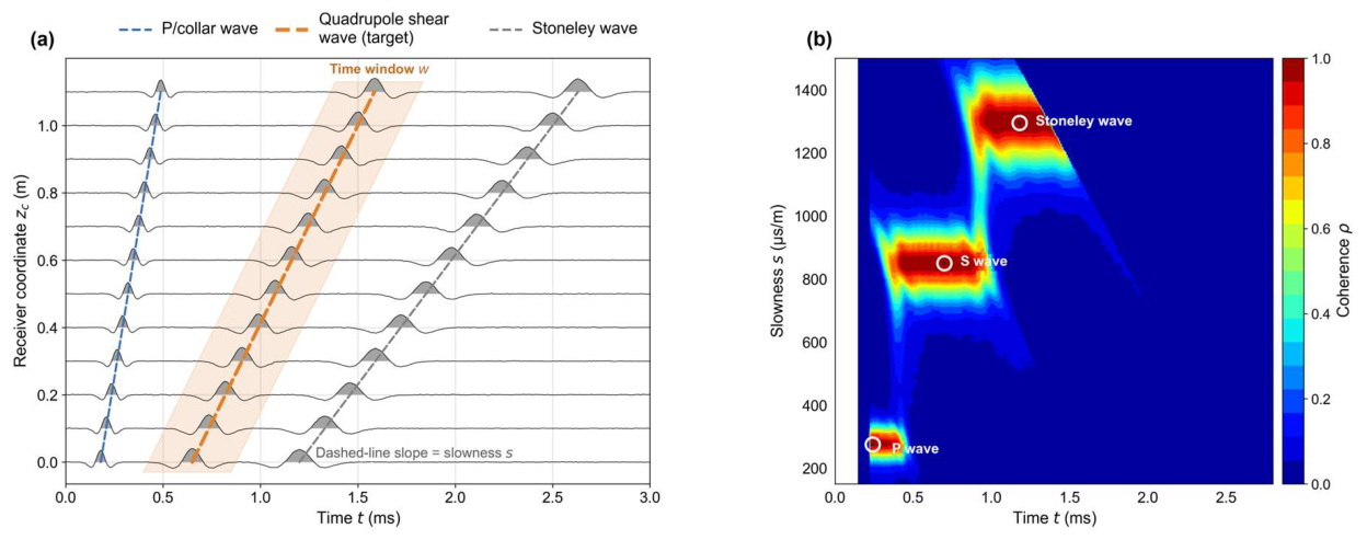
Figure 2.
Overall processing pipeline from array gathers to shear-wave velocity extraction.
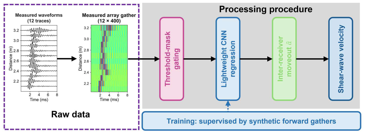
Figure 3.
Architecture of the regression CNN.
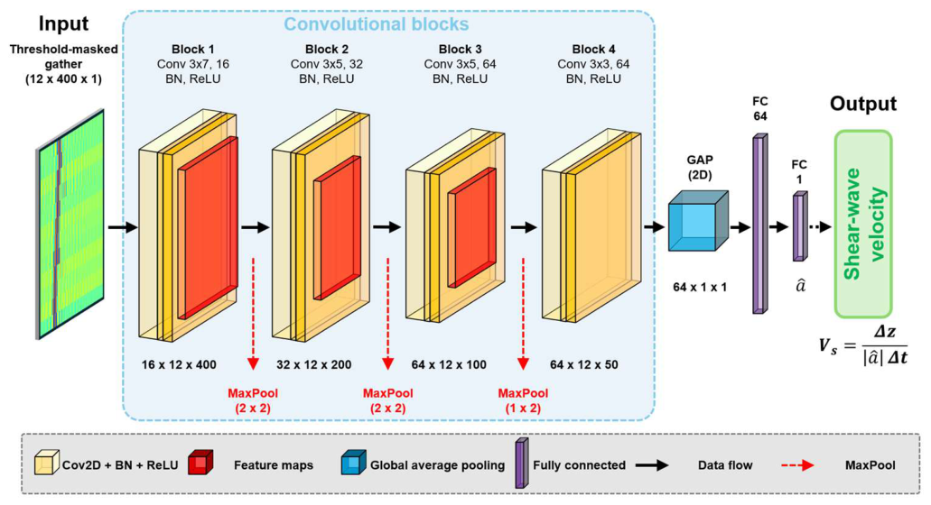
Figure 4.
Morphological comparison between synthetic training gathers and measured gathers.
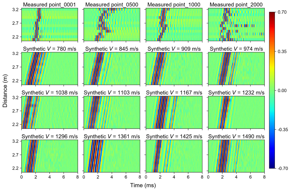
Figure 5.
Five-fold cross-validation of the synthetically supervised regression. (a) Median relative velocity error of each fold. (b) Fraction of samples with velocity errors ≤5% and ≤10% in each fold.
Figure 5.
Five-fold cross-validation of the synthetically supervised regression. (a) Median relative velocity error of each fold. (b) Fraction of samples with velocity errors ≤5% and ≤10% in each fold.
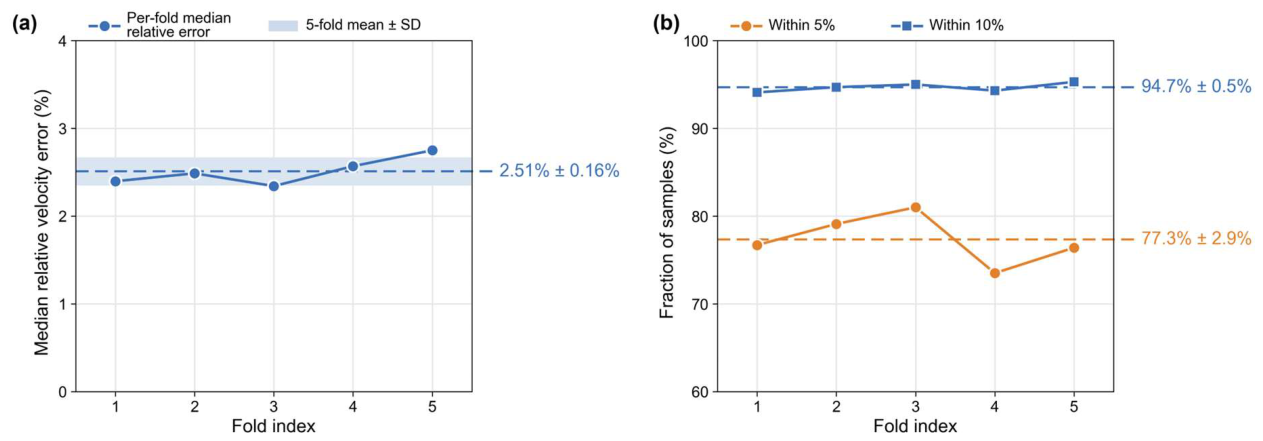
Figure 6.
Comprehensive evaluation of the inter-receiver moveout regression CNN on the synthetic test set. (a) Scatter plot of predicted versus true velocity. (b) Histogram of relative error with a normal fit. (c) Cumulative distribution of relative error.
Figure 6.
Comprehensive evaluation of the inter-receiver moveout regression CNN on the synthetic test set. (a) Scatter plot of predicted versus true velocity. (b) Histogram of relative error with a normal fit. (c) Cumulative distribution of relative error.
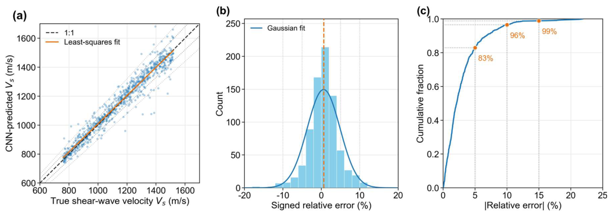
Figure 7.
Shear-wave velocity extraction on the measured well interval. (a) Waveform pixel image. (b) Input after threshold masking (). (c) Shear-wave velocity log. (d) Inter-receiver moveout histogram. (e) Shear-wave velocity histogram. (f) Hyperbolic velocity–moveout relation.
Figure 7.
Shear-wave velocity extraction on the measured well interval. (a) Waveform pixel image. (b) Input after threshold masking (). (c) Shear-wave velocity log. (d) Inter-receiver moveout histogram. (e) Shear-wave velocity histogram. (f) Hyperbolic velocity–moveout relation.
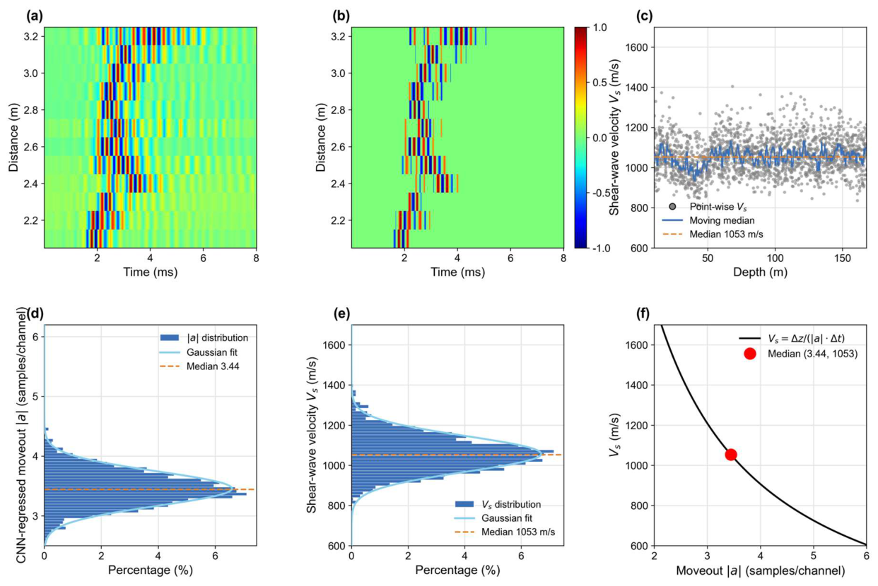
Figure 8.
Cross-domain and cross-processing consistency.
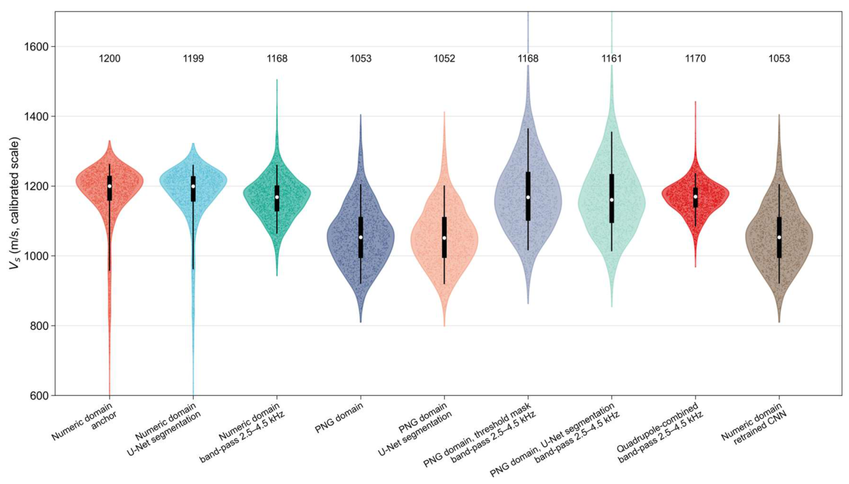
Figure 9.
Comparison between the threshold mask and the Attention U-Net segmentation mask.
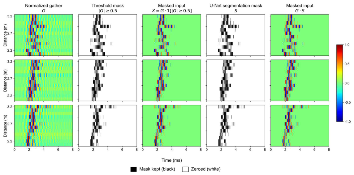
Figure 10.
Examples of CNN regression-based extraction on image-inversion-domain gathers.
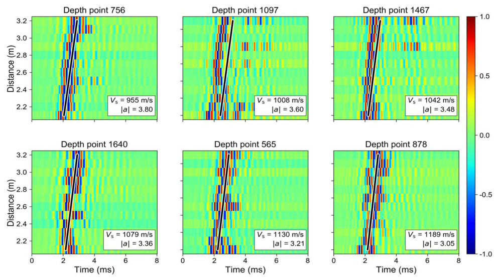
Figure 11.
Comparison between the measured-STC-supervised variant and the measured STC curve. (a) Velocity curves: CNN versus measured STC. (b) The most informative well interval. (c) Velocity distributions: CNN versus measured STC.
Figure 11.
Comparison between the measured-STC-supervised variant and the measured STC curve. (a) Velocity curves: CNN versus measured STC. (b) The most informative well interval. (c) Velocity distributions: CNN versus measured STC.
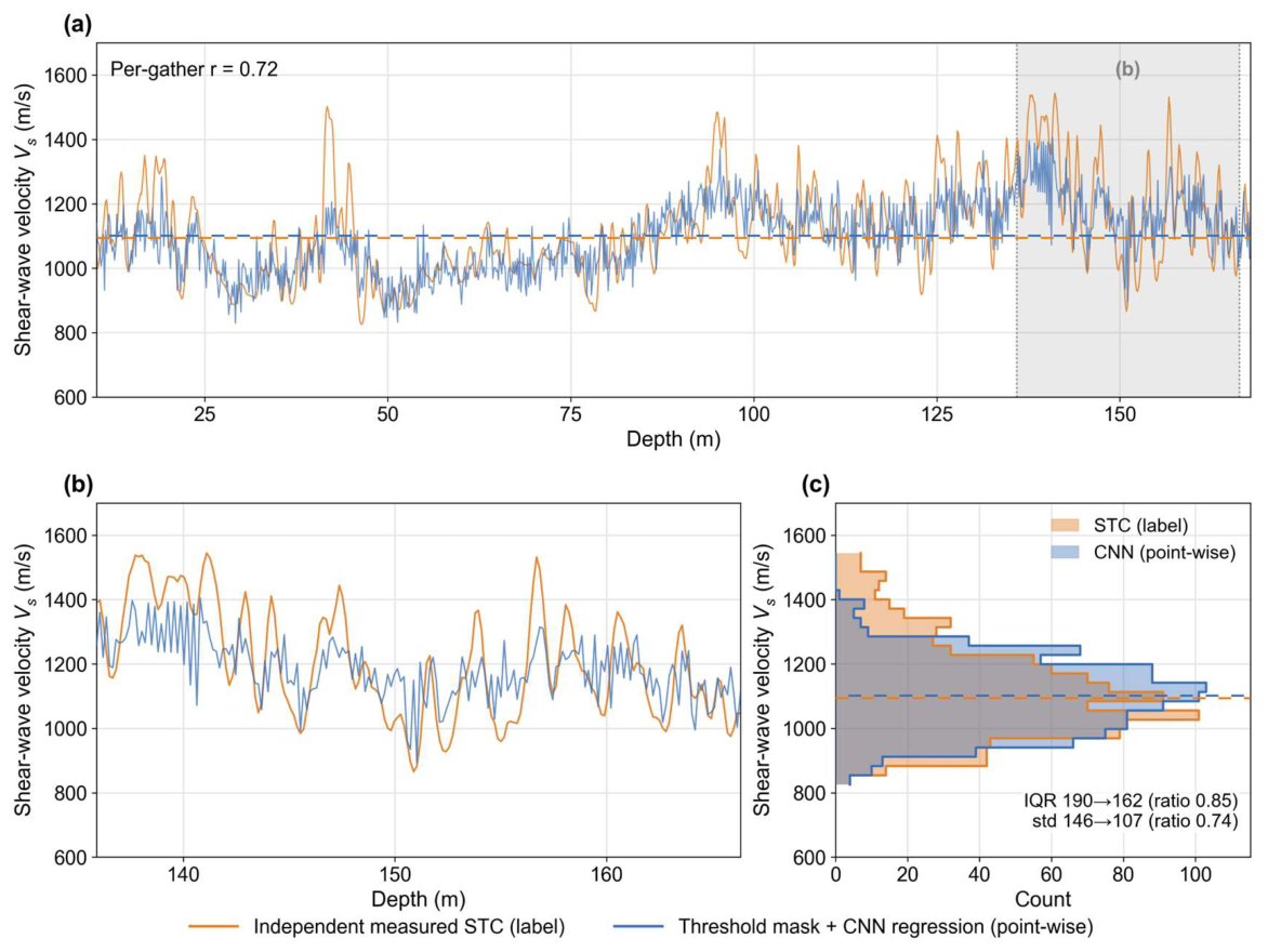
Figure 12.
Error structure and velocity-dependent bias of the comparison variant. (a) Binned median of the signed relative error. (b) Signed bias for the slow/intermediate/fast terciles. (c) Histogram of the residual CNN − measured STC.
Figure 12.
Error structure and velocity-dependent bias of the comparison variant. (a) Binned median of the signed relative error. (b) Signed bias for the slow/intermediate/fast terciles. (c) Histogram of the residual CNN − measured STC.
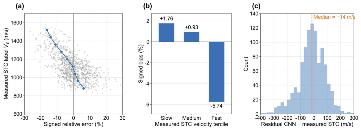
Figure 13.
Outlier suppression by the comparison variant. (a) Measured STC and CNN velocity curves within a depth interval. (b) Median residuals about the local trend. (c) Distribution of between adjacent depths.
Figure 13.
Outlier suppression by the comparison variant. (a) Measured STC and CNN velocity curves within a depth interval. (b) Median residuals about the local trend. (c) Distribution of between adjacent depths.
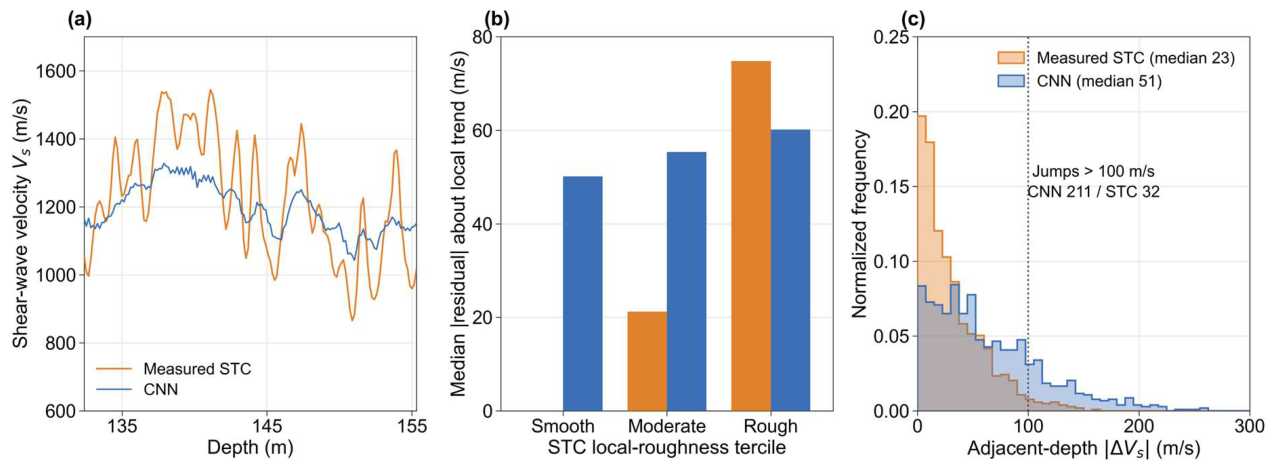

Table 1.
Acquisition and processing constants.
| Quantity | Symbol | Value |
| Number of receiver channels | Nch | 12 |
| Nominal receiver spacing | Δznom | 0.1 m |
| Time sampling interval | Δt | 20 µs |
| Time samples used per trace | Nt | 400 |
| Threshold-mask level | θ | 0.5 (normalized amplitude) |
| Number of measured numeric-domain gathers | — | 2198 (consecutive depths) |
| Synthetic training / validation / test split | — | 4000 / 800 / 800 |
| Measured STC comparison-label gathers | — | 1032 (80/20 = 826/206) |
| STC reference search: velocity range / step | — | 1000–3500 m/s / 25 m/s |
| STC reference search: time window | — | 45 samples (0.9 ms) |
Table 2.
Architecture of the regression CNN.
| Layer | Kernel / units | Output size |
| Input | — | 12 × 400 × 1 |
| Conv + BN + ReLU | 3 × 7, 16 | 12 × 400 × 16 |
| MaxPool | 2 × 2, stride 2 | 6 × 200 × 16 |
| Conv + BN + ReLU | 3 × 5, 32 | 6 × 200 × 32 |
| MaxPool | 2 × 2, stride 2 | 3 × 100 × 32 |
| Conv + BN + ReLU | 3 × 3, 64 | 3 × 100 × 64 |
| MaxPool | 1 × 2, stride [12] | 3 × 50 × 64 |
| Conv + BN + ReLU | 3 × 3, 64 | 3 × 50 × 64 |
| Global average pooling | — | 64 |
| Fully connected + ReLU | 64 | 64 |
| Fully connected (linear) | 1 | 1 (â, samples/channel) |
Table 3.
Comprehensive evaluation metrics of the inter-receiver moveout regression CNN on the synthetic held-out test set.
Table 3.
Comprehensive evaluation metrics of the inter-receiver moveout regression CNN on the synthetic held-out test set.
| Metric | Value |
| Coefficient of determination R² | 0.947 |
| Pearson correlation coefficient r | 0.974 |
| Spearman rank correlation ρ | 0.975 |
| Concordance correlation coefficient CCC | 0.973 |
| Root-mean-square error RMSE (m/s) | 51 |
| Mean absolute error MAE (m/s) | 35 |
| Mean absolute percentage error MAPE (%) | 3.02 |
| Median relative error (%) | 2.11 |
| Signed median bias (%) | +0.63 |
| Fraction within 5% / 10% / 15% (%) | 83.0 / 96.5 / 98.9 |
| Gross-error (>20%) fraction (%) | 0.50 |
| P90 / P95 |relative error| (%) | 6.8 / 9.0 |
Table 4.
Comparison between the measured-STC-supervised comparison variant and classical regression models.
Table 4.
Comparison between the measured-STC-supervised comparison variant and classical regression models.
| Model | Random MRE | Random r | Blocked MRE | Blocked r |
| CNN threshold-mask (comparison variant) | 7.22% | 0.53 | 11.93% | 0.20 |
| ExtraTrees(300) | 5.57% | 0.66 | 8.94% | 0.13 |
| Random forest RF(300) | 6.79% | 0.62 | 8.80% | 0.14 |
| HistGBM | 6.56% | 0.62 | 9.07% | 0.16 |
| SVR(RBF) | 6.78% | 0.57 | 9.66% | 0.11 |
| Ridge regression | 6.82% | 0.56 | 10.24% | 0.04 |
| Constant baseline | 9.03% | — | 9.50% | — |
Table 5.
Computational cost of the CNN and the vectorized STC.
| CNN | STC | |
| Parameters / size | 0.068 M / 266 KB | — |
| Runtime for 1032 gathers | 26 ± 0.4 ms (GPU) | 640 ms |
| Per gather | 0.025 ms | 0.62 ms |
| Relative speed-up | ≈25× | 1× |
Disclaimer/Publisher’s Note: The statements, opinions and data contained in all publications are solely those of the individual author(s) and contributor(s) and not of MDPI and/or the editor(s). MDPI and/or the editor(s) disclaim responsibility for any injury to people or property resulting from any ideas, methods, instructions or products referred to in the content. |
© 2026 by the authors. Licensee MDPI, Basel, Switzerland. This article is an open access article distributed under the terms and conditions of the Creative Commons Attribution (CC BY) license.
Copyright: This open access article is published under a Creative Commons CC BY 4.0 license, which permit the free download, distribution, and reuse, provided that the author and preprint are cited in any reuse.