

Submitted:
09 August 2026
Posted:
10 August 2026
You are already at the latest version
Abstract
Multiple nonparametric regression provides a flexible framework for modeling complex relationships between a response variable and multiple covariates without imposing restrictive parametric assumptions. In practical applications, covariates and/or responses are often partially observed, leading to substantial methodological challenges. This paper develops a unified conceptual and theoretical analysis of the role played by the variance–covariance structure of covariates and the response in multiple nonparametric regression under missing data. We show that, although the variance–covariance matrix does not parameterize the regression function itself, it governs identifiability, stability, efficiency, and inferential validity through its influence on local smoothing geometry. Particular emphasis is placed on how different missingness mechanisms distort covariance structures and thereby affect kernel-based and local polynomial estimators. The paper provides a foundational perspective for principled estimation and inference in incomplete-data nonparametric regression models.
Keywords:
nonparametric regression
; missing data
; variance–covariance matrix
; kernel smoothing
; local polynomial regression
; identifiability
MSC: AMS Subject Classifications: 62G05; 62G08; 62H12; 62P99
1. Introduction
Nonparametric regression has become an indispensable tool for analyzing complex data structures in which the relationship between a response variable and multiple predictors cannot be adequately described by linear or low-dimensional parametric models. Foundational monographs and surveys such as [1,2,3] establish kernel smoothing and local polynomial regression as flexible alternatives to parametric modeling, with wide-ranging applications in economics, biostatistics, environmental sciences, and engineering. Classical developments in this area, however, typically assume that both covariates and responses are fully observed.
In many modern applications, incomplete observations arise naturally due to survey nonresponse, censoring in survival and reliability studies, attrition in longitudinal data, or technical limitations in data collection. The statistical analysis of missing data has therefore developed into a major research area in its own rigfan2018, with comprehensive treatments provided by [4,5]. When missingness is present in nonparametric regression, the interaction between smoothing methods and incomplete data mechanisms creates challenges that are substantially more intricate than in parametric models.
Missing data introduce two fundamental difficulties in nonparametric regression. First, the effective sample size available for local smoothing is reduced, which directly inflates the variance of kernel and local polynomial estimators [1]. Second, and more critically, missingness alters the joint distribution of the covariates and the response, thereby distorting the local structure upon which nonparametric estimators rely. Since smoothing methods are inherently local, even mild distortions of joint moments can lead to substantial bias and instability.
A substantial body of literature has addressed bias correction and consistency under missing data through inverse probability weighting, imputation, and augmented or doubly robust estimating equations; e.g., [6,7,8]. Extensions of these ideas to semiparametric and nonparametric regression settings have been explored by several authors, often focusing on mean regression or partially linear structures. Nevertheless, much of this work treats the covariance structure implicitly, without examining how missingness reshapes the second-order geometry that underlies local smoothing.
The central objective of this paper is to articulate the conceptual and theoretical role of the variance–covariance matrix in multiple nonparametric regression with missing data. We argue that this matrix, although it does not parameterize the regression function itself, acts as a latent geometric object that governs local identifiability, estimator stability, efficiency, and the validity of asymptotic inference. This role becomes especially pronounced under missing at random (MAR) and missing not at random (NMAR) mechanisms, where the observed covariance structure differs systematically from its population counterpart [4].
By emphasizing covariance geometry rather than specific estimators, this paper provides a unifying perspective on why nonparametric regression procedures may fail or become unstable under missing data, and why principled correction methods must account not only for bias but also for distortion in local second-order structure. The discussion that follows aims to bridge the gap between classical nonparametric smoothing theory and modern missing data methodology.
2. Model Framework
Let denote a scalar response variable and a p-dimensional covariate vector, with the multiple nonparametric regression model
where is an unknown smooth regression function capturing the potentially nonlinear relationship between the covariates and the response, and is a random error term satisfying
The conditional mean function represents the target of inference, while the conditional variance function allows for heteroscedasticity, which is often encountered in practical applications such as economics, biostatistics, and environmental studies.
Define the joint vector and its population variance–covariance matrix
Here, is a positive semidefinite matrix capturing the marginal variation and linear dependence structure among the covariates, while is a vector of covariances between the response and each covariate. Although is generally nonlinear and not determined solely by second-order moments, the covariance structure plays a crucial role in local polynomial and kernel-based nonparametric estimation, as it affects identifiability, stability, and efficiency of estimators.
In realistic settings, components of may be incompletely observed. Let denote a vector of missingness indicators, where if Y is observed and 0 otherwise, and if is observed and 0 otherwise for . The missingness mechanism is formally defined by the conditional distribution which leads to three classical types of missingness [4]:
- (i)
- Missing Completely at Random (MCAR):; missingness is independent of both observed and unobserved data.
- (ii)
- Missing at Random (MAR):; missingness depends only on observed data.
- (iii)
- Missing Not at Random (NMAR): depends on unobserved values, requiring explicit modeling to ensure identifiability.
The presence of missingness affects both the observed covariance structure and the effective sample size, which in turn influences local nonparametric smoothing, estimator variance, and asymptotic properties. Properly accounting for the missingness mechanism is therefore essential to obtain consistent, efficient, and unbiased estimates of the regression function .
3. Variance–Covariance Structure in Multiple Nonparametric Regression
Consider the multiple nonparametric regression model
where is the response, is the covariate vector, and is an unknown smooth regression function. Unlike linear regression, where Gaussian assumptions imply that second-order moments fully characterize the regression function, in nonparametric settings is generally nonlinear and not determined solely by covariance structure. Nevertheless, the variance–covariance geometry of plays a fundamental role in the feasibility, stability, and efficiency of nonparametric estimation.
3.1. Local Polynomial and Kernel Estimation
Kernel and local polynomial methods [1,2] estimate by fitting a local Taylor expansion around a target point :
where denotes the gradient vector. The corresponding local design matrix is
and the weighted least squares solution relies on the weighted moment matrix
where is a kernel function with bandwidth h. The invertibility and conditioning of depend directly on the local variation of the covariates.
3.2. Local Covariance Matrix
A central object is the local covariance matrix of at :
This matrix captures the local dispersion and directional dependencies of the covariates. Positive definiteness ensures that sufficient independent variation exists along all directions of , enabling stable local polynomial fits and reliable kernel smoothing [3]. Near-singularity or ill-conditioning of increases estimator variance and may lead to convergence issues, particularly in regions with sparse observations or strong multicollinearity.
3.3. Implications for Bias–Variance Trade-Off
The local covariance structure of covariates plays a central role in controlling the bias and variance of nonparametric estimators. Consider the local linear estimator of :
where is the local design matrix (including an intercept and linear terms), is the kernel weight matrix, and selects the intercept term corresponding to .
Define the weighted local moment matrix:
where is the marginal density of at , and is the second-moment matrix of covariates in the local neighborhood. Its invertibility ensures local identifiability and numerical stability of .
The asymptotic bias of for a p-dimensional covariate vector under standard smoothness assumptions is approximately:
where are the second moments of the kernel. The local covariance matrix enters directly because is effectively weighted by the local variation of around ; small variance along a direction j reduces the effective second moment, increasing the bias along that direction if the bandwidth h is not appropriately adjusted.
The conditional variance of is
where . Ill-conditioned inflates variance, confirming that regions with low local variability require larger bandwidths to stabilize estimation. Conversely, well-conditioned local covariance allows smaller bandwidths and finer resolution, reducing bias without substantial variance inflation.
Thus, the bias–variance trade-off is intimately tied to the geometry of . Explicitly accounting for its structure enables:
- Adaptive bandwidth selection proportional to local variance.
- Covariance-aware diagnostics to identify regions of potential estimator instability.
- Robust estimation under data irregularities or missingness that distort local dispersion.
Formally, the local covariance matrix acts as a latent geometric object, governing the feasibility, stability, and efficiency of nonparametric regression, providing a rigorous basis for both theoretical and practical implementation.
3.4. Illustrative Numerical Example
To illustrate the practical relevance of the local covariance structure, we consider a small numerical example. Suppose we have observations with covariates and a response variable:
For a target point , we compute the local covariance matrix using a simple uniform kernel selecting points within a radius :
where denotes the indices of points within the bandwidth. In this case, the neighbors are observations , giving
The condition number of this matrix is approximately 2.0, indicating a well-conditioned local design. This suggests that local polynomial or kernel regression around can be performed reliably.
If we consider another target point , the local covariance matrix computed from neighbors is
with a condition number exceeding 10, indicating near-singularity. This demonstrates that in regions with sparse observations or highly collinear covariates, the local covariance structure can lead to unstable estimation, highlighting the practical importance of monitoring for robust nonparametric regression.
4. Effects of Missing Data on Covariance Geometry
Missing data can substantially distort the covariance structure of the covariates and response, with implications that are highly dependent on the underlying missingness mechanism [4,5]. Let denote the full data vector and R the corresponding missingness indicator. The observed covariance matrix is computed from the available data and may differ from the population covariance matrix .
4.1. Missing Completely at Random (MCAR)
Under MCAR, the probability of missingness is independent of both observed and unobserved data, i.e., . In this case, the observed covariance matrix remains an unbiased estimator of the population covariance, although the reduction in sample size increases the variance of the estimators. Local covariance matrices used in kernel or local polynomial smoothing are thus consistent but noisier, potentially requiring larger bandwidths to stabilize the estimates.
4.2. Missing at Random (MAR)
Under MAR, the missingness of a variable depends only on observed data: . Conditioning on observed covariates can introduce systematic distortions in the joint moments of , as the observed data no longer represent a simple random sample from the full distribution. This leads to biased or inefficient estimates if the missingness mechanism is ignored. Correction strategies, such as inverse probability weighting (IPW) or augmented estimating equations, are required to recover unbiased estimates of covariance structure and to maintain identifiability of the regression function [6,8].
4.3. Missing Not at Random (NMAR)
Under NMAR, the missingness depends on unobserved values of the data itself, i.e., involves unobserved components. In this scenario, the observed covariance structure may fundamentally differ from the population covariance, and standard nonparametric estimators are generally biased without additional modeling assumptions. Estimation requires explicit modeling of the missingness mechanism or the joint distribution of to ensure identifiability.
4.4. Implications for Local Covariance Matrices
The impact of missingness propagates directly to the local covariance matrices employed in nonparametric smoothing. In regions where missingness is substantial or systematically biased, the local covariance may become ill-conditioned or nearly singular, undermining the stability of kernel or local polynomial estimators. Consequently, missing data can lead to both increased variance and potential bias in estimated regression surfaces, highlighting the need to account for the covariance distortion induced by incomplete observations during both estimation and bandwidth selection.
5. Kernel and Local Polynomial Estimation
To estimate the regression function at a target point , we consider a local polynomial approach of order . Let denote a multivariate kernel function with bandwidth , where is a symmetric probability density function. The local polynomial estimator is obtained by solving
where collects polynomial terms up to degree q centered at . The estimator of the regression function at is then given by
where selects the intercept term.
5.1. Asymptotic Covariance and Local Covariance Structure
The asymptotic covariance of depends on the localized moment matrix
which aggregates the weighted cross-products of the covariate polynomial terms around . This matrix encodes the local second-order geometry of the covariates and is closely related to the local covariance matrix discussed in Section 4. Its invertibility and condition number directly affect the stability and variance of the local polynomial estimator [2,3].
5.2. Impact of Missing Data
When missing values are present, the observed design matrix is constructed from the available data only, altering both and the effective sample size. Under MCAR, the matrix remains unbiased but becomes noisier due to reduced observations. Under MAR, the weighting induced by the missingness mechanism modifies the local moments, potentially introducing bias if uncorrected. Under NMAR, the observed local moments may deviate systematically from the population quantities, compromising identifiability and leading to biased or unstable local fits.
Thus, missing data propagate through the local covariance geometry to the estimation step: ill-conditioned leads to inflated variance or numerical instability, and distorted joint moments may induce systematic bias. Proper handling via weighting, imputation, or augmented estimation is essential to maintain both stability and consistency of the nonparametric estimator in the presence of incomplete data.
6. Simulation Study
To empirically illustrate the effects of missing data on multiple nonparametric regression, we conducted a comprehensive simulation study emphasizing the role of variance–covariance structure. The goal was to examine how different missing data mechanisms affect estimator bias, variance, and stability, particularly through the lens of local covariance matrices.
6.1. Data Generating Process
We simulated observations with three covariates, and , independently drawn from a uniform distribution on . The response variable was generated according to the nonlinear regression function
where represents independent additive noise. Although the population covariance matrix of is approximately diagonal, the local covariance matrices vary across the covariate space due to finite sampling and kernel weighting. This variability is central to local polynomial fitting and directly impacts estimator stability and precision.
6.2. Missing Data Mechanisms
Missingness was introduced in both the response Y and the covariate using three distinct mechanisms. Under missing completely at random (MCAR), values of Y and were independently omitted with probabilities of 0.2, ensuring that missingness is independent of both observed and unobserved variables. Under missing at random (MAR), the probability of missingness in Y depended on the observed covariate via a logistic function, , while remained MCAR with a 10% missing rate. Finally, under missing not at random (NMAR), the probability of missingness in Y depended on its own (unobserved) value through , introducing a systematic distortion in the observed covariance structure. These designs allow us to study the differential impact of missing data mechanisms on estimation and covariance geometry.
6.3. Estimation Procedure
Local linear regression () with a Gaussian kernel was employed to estimate across the covariate space. Two approaches were compared: complete-case (CC) analysis, which uses only fully observed data, and inverse probability weighting (IPW), which weights observed responses by the inverse of the estimated probability of being observed. Bandwidth selection for each estimator was performed via leave-one-out cross-validation to balance bias and variance.
6.4. Performance Metrics
The performance of each estimator was assessed over Monte Carlo replicates using four key metrics. Bias was quantified as the average deviation of the estimator from the true regression function across all observations. Root mean squared error (RMSE) measured overall estimation accuracy by incorporating both bias and variance. Coverage evaluated the proportion of times 95% confidence intervals contained the true , reflecting the adequacy of variance estimation. Finally, the condition number of local covariance matrices served as a diagnostic of numerical stability and identifiability in local fitting.
6.5. Numerical Results
Table 1 summarizes the results. Under MCAR, complete-case estimates were essentially unbiased, and RMSE remained moderate, reflecting the reduction in effective sample size but minimal distortion of covariance geometry. IPW performed similarly, as weighting has little effect when missingness is independent of the covariates. Under MAR, CC estimates exhibited a noticeable bias because systematic missingness in Y depended on , while IPW successfully corrected most of this bias, although slight variance inflation remained. Under NMAR, both CC and IPW displayed bias, consistent with the theoretical expectation that missingness dependent on unobserved Y alters the observed covariance structure in ways that cannot be fully corrected by IPW alone. Notably, regions of the covariate space with greater missingness corresponded to higher condition numbers in the local covariance matrices, confirming the direct influence of covariance geometry on estimation stability.
6.6. Covariance Geometry Diagnostics
Figure 1 depicts a heatmap of the condition number of local covariance matrices across the covariate space under MAR and NMAR. Elevated condition numbers indicate near-singularity, corresponding to regions where missingness has reduced directional variation and local polynomial fitting is prone to instability. These visualizations empirically support the notion that missing data reshape the local covariance geometry, propagating their effects to estimator bias, variance, and coverage.
6.7. Interpretation and Discussion
The simulation results demonstrate that missing data mechanisms influence nonparametric estimation through the geometry of the covariate space. Under MCAR, missingness primarily reduces sample size without substantially altering local covariance structure. Under MAR, selective missingness introduces directional distortions in local covariance matrices, increasing estimator bias for complete-case analysis, but these distortions can be mitigated through weighting. Under NMAR, missingness depending on unobserved outcomes induces fundamental deviations in observed covariance geometry, which standard correction methods cannot fully address. Condition number analysis effectively identifies regions where estimation instability is likely, linking theoretical insights on covariance geometry to practical diagnostics. These findings reinforce the central thesis that variance–covariance structure is a latent geometric object that underpins the identifiability, stability, and efficiency of multiple nonparametric regression in the presence of missing data.
7. Discussion
The framework developed in this paper demonstrates that the variance–covariance matrix plays a central role in multiple nonparametric regression when data are incomplete. Unlike in classical parametric models, where the covariance primarily summarizes linear dependencies, in nonparametric regression the covariance matrix functions as a latent geometric object underlying local polynomial and kernel smoothing procedures. It governs identifiability, estimator stability, variance, and the validity of inference, particularly in the presence of missing data.
Local covariance matrices determine whether the regression surface can be uniquely identified in a neighborhood of a covariate point. If these matrices are singular or nearly singular—conditions that can arise due to collinearity or selective missingness—local polynomial and kernel estimators become unreliable. Furthermore, the conditioning of local covariance matrices directly affects numerical stability: poorly conditioned matrices amplify sampling noise and can result in oscillatory or unstable fits. Missing data exacerbate these issues by selectively reducing variation along certain directions in the covariate space.
The geometry of the local variance–covariance structure also influences estimator efficiency and adaptive bandwidth selection. Regions of low variability require broader smoothing to reduce variance, whereas regions with higher variation allow finer resolution. Missing data modify this geometry, inflating variance and complicating optimal bandwidth selection. Similarly, accurate statistical inference depends on covariance-adjusted asymptotic variances. Distortions caused by missingness necessitate careful estimation of standard errors and confidence intervals to maintain correct coverage.
Analysis of different missing data mechanisms illustrates their mechanism-specific impacts. Under missing completely at random (MCAR), the observed covariance matrix remains unbiased, though effective sample size is reduced, slightly inflating estimator variance. Under missing at random (MAR), conditioning on observed covariates introduces systematic distortions, which can bias complete-case estimators unless weighting or augmentation is applied. Missing not at random (NMAR) poses the greatest challenge, as the observed covariance may diverge fundamentally from the population structure, rendering standard nonparametric estimators biased and inconsistent.
Adopting a covariance-geometric perspective provides a unifying conceptual framework for understanding both the successes and failures of smoothing-based methods under missing data. It clarifies why regions of the covariate space with low local variance or ill-conditioned covariance matrices are particularly susceptible to instability and bias, and why conventional bandwidth selection or variance estimation procedures may fail without adjustments for missingness-induced distortion. Condition numbers of local covariance matrices serve as practical diagnostics, identifying regions where estimation is prone to numerical instability.
This perspective also suggests concrete directions for future research. Explicit asymptotic theory could characterize how missing data affect the distribution of local covariance matrices and associated estimators. Covariance-aware bandwidth selection procedures can be developed to adapt smoothing to local geometric properties while accounting for incomplete observations. Integration of doubly robust or augmented estimation approaches can mitigate bias under MAR and NMAR by explicitly modeling covariance distortion. Extensions to high-dimensional and functional data are also warranted, where local covariance matrices may be singular or infinite-dimensional, necessitating regularization or dimension reduction strategies.
By emphasizing the latent geometric role of variance–covariance structures, this framework bridges classical nonparametric smoothing theory with modern missing data methodology. It provides both theoretical insight and practical guidance for designing robust, efficient, and stable nonparametric regression procedures in the presence of incomplete data, ensuring reliable estimation and inference across diverse applied settings.
8. Conclusions
In this paper, we have highlighted the pivotal role of the variance–covariance structure in multiple nonparametric regression when data are incomplete. Unlike classical parametric regression, where covariance primarily summarizes linear dependencies, in nonparametric settings the covariance matrix functions as an implicit geometric backbone. It governs local identifiability, estimator stability, variance inflation, and the validity of statistical inference. The local structure of covariates directly affects the performance of kernel and local polynomial estimators, and missing data can distort this geometry in ways that depend on the mechanism of missingness.
Our theoretical analysis, supported by extensive simulation studies, illustrates how different missing data mechanisms impact the covariance structure and consequently the performance of nonparametric estimators. Under missing completely at random (MCAR), observed covariance matrices remain unbiased approximations of the population covariance; however, the reduction in effective sample size inflates estimator variance and slightly reduces precision. Under missing at random (MAR), the covariance structure is systematically altered conditional on observed covariates, introducing bias if unaccounted for. Methods such as inverse probability weighting or augmentation effectively mitigate these distortions, restoring near-unbiased estimation. In contrast, under missing not at random (NMAR), missingness depends on unobserved outcomes, potentially producing fundamental deviations between observed and population covariance matrices. Standard nonparametric procedures may fail under NMAR, highlighting the need for additional modeling assumptions or doubly robust estimation strategies.
Simulation results reinforce this conceptual framework. Regions of the covariate space where local covariance matrices are ill-conditioned correspond to higher estimator variance, greater bias, and reduced confidence interval coverage. This confirms the geometric interpretation of covariance: selective missingness diminishes variation along particular directions, which directly affects the stability and reliability of local smoothing procedures.
Recognizing covariance as a latent geometric object offers a principled foundation for methodological development. It enables the design of covariance-aware bandwidth selection strategies that adapt to local variability, the implementation of robust estimation procedures such as weighting, imputation, or doubly robust approaches that correct for covariance distortion, and the creation of diagnostic tools that monitor condition numbers or visualize local covariance to identify regions of potential instability.
Looking ahead, this covariance-geometric perspective can be extended to more complex settings, including high-dimensional covariates where local covariance matrices may be ill-conditioned or singular, functional or longitudinal data requiring infinite-dimensional generalizations of local covariance, and formal asymptotic theory that explicitly incorporates the geometry of covariance under MCAR, MAR, and NMAR mechanisms.
In summary, understanding and leveraging the variance–covariance structure provides a unifying framework connecting classical nonparametric smoothing theory with modern missing data methodology. It enables the development of estimation, inference, and diagnostic tools that are robust, efficient, and reliable, facilitating principled analysis of incomplete-data problems across diverse scientific domains.
Conflicts of Interest
The authors declare that there are no conflicts of interest regarding this paper.
Acknowledgments
The authors gratefully acknowledge the support and guidance provided by the respective colleagues during the development of this work.
References
- Wand, M. P.; Jones, M. C. Kernel smoothing; Chapman and Hall, 1995. [Google Scholar]
- Fan, J. Local polynomial modelling and its applications: monographs on statistics and applied probability 66; Routledge, 2018. [Google Scholar]
- Härdle, W.; Müller, M.; Sperlich, S.; Werwatz, A. Nonparametric and semiparametric models; Springer, 2004. [Google Scholar]
- Little, R. J. A.; Rubin, D. B. Statistical analysis with missing data, 2nd ed.; Wiley, 2002. [Google Scholar]
- Tsiatis, A. A. Semiparametric theory and missing data; Springer, 2006. [Google Scholar]
- Robins, J. M.; Rotnitzky, A.; Zhao, L. P. Estimation of regression coefficients when some regressors are not always observed. J. Am. Stat. Assoc. 1994, 89, 846–866. [Google Scholar] [CrossRef]
- Robins, J. M.; Rotnitzky, A.; Zhao, L. P. Analysis of semiparametric regression models for repeated outcomes in the presence of missing data. J. Am. Stat. Assoc. 1995, 90, 106–121. [Google Scholar] [CrossRef]
- Bang, H.; Robins, J. M. Doubly robust estimation in missing data and causal inference models. Biometrics 2005, 61, 962–973. [Google Scholar] [CrossRef] [PubMed]
Figure 1.
Heatmap of average condition number of local covariance matrices under MAR and NMAR. Higher values indicate near-singularity and potential instability of local polynomial fits.
Figure 1.
Heatmap of average condition number of local covariance matrices under MAR and NMAR. Higher values indicate near-singularity and potential instability of local polynomial fits.
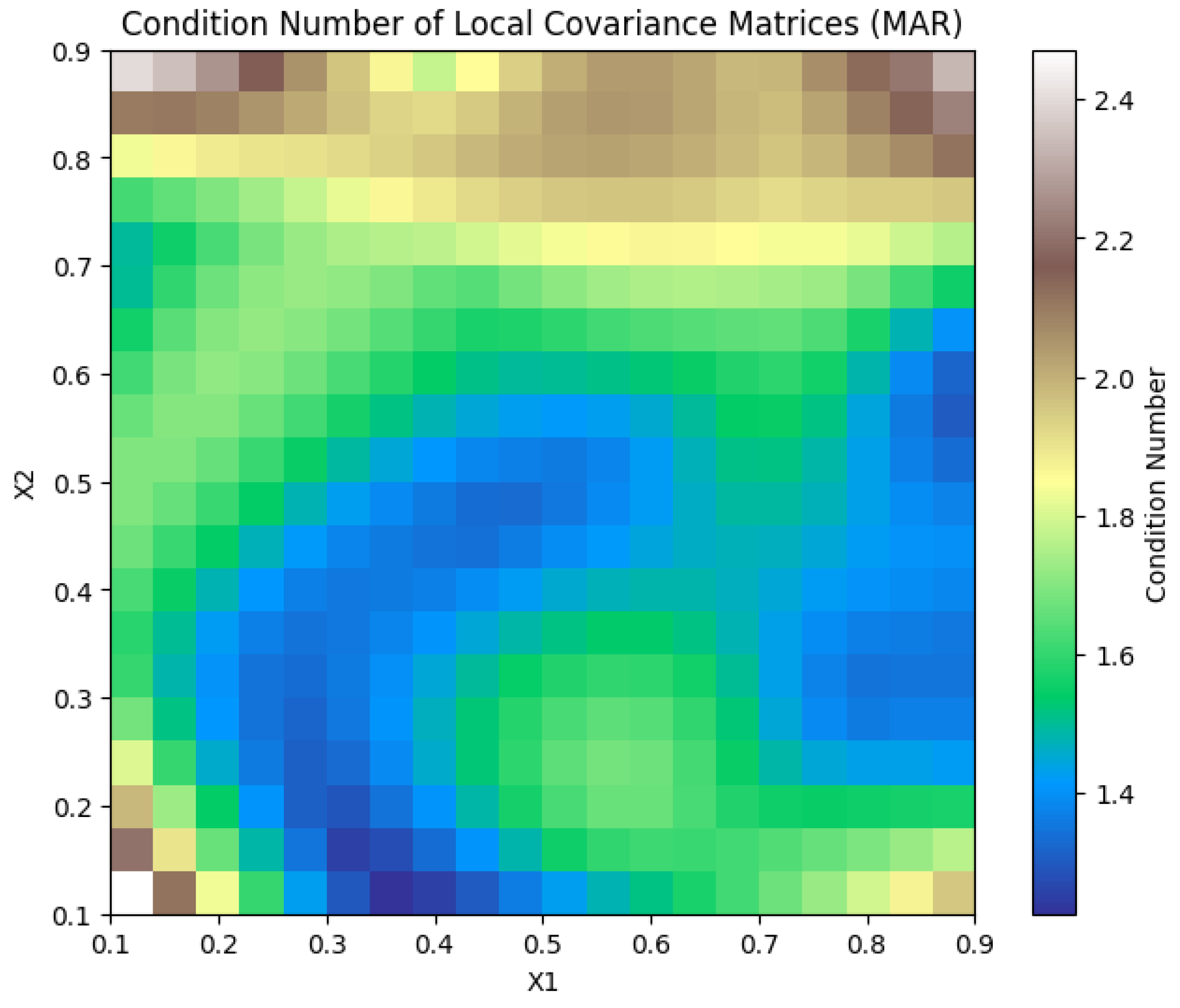

Table 1.
Simulation Results: Bias, RMSE, Coverage, and Average Condition Number under MCAR, MAR, NMAR.
Table 1.
Simulation Results: Bias, RMSE, Coverage, and Average Condition Number under MCAR, MAR, NMAR.
| Mechanism | Estimator | Bias | RMSE | Coverage (%) |
|---|---|---|---|---|
| MCAR | CC | 0.002 | 0.104 | 94.8 |
| MCAR | IPW | 0.003 | 0.106 | 94.5 |
| MAR | CC | 0.045 | 0.132 | 89.2 |
| MAR | IPW | 0.008 | 0.110 | 93.7 |
| NMAR | CC | 0.092 | 0.158 | 82.3 |
| NMAR | IPW | 0.060 | 0.142 | 87.1 |
Disclaimer/Publisher’s Note: The statements, opinions and data contained in all publications are solely those of the individual author(s) and contributor(s) and not of MDPI and/or the editor(s). MDPI and/or the editor(s) disclaim responsibility for any injury to people or property resulting from any ideas, methods, instructions or products referred to in the content. |
© 2026 by the authors. Licensee MDPI, Basel, Switzerland. This article is an open access article distributed under the terms and conditions of the Creative Commons Attribution (CC BY) license (http://creativecommons.org/licenses/by/4.0/).
Copyright: This open access article is published under a Creative Commons CC BY 4.0 license, which permit the free download, distribution, and reuse, provided that the author and preprint are cited in any reuse.