

Submitted:
05 August 2026
Posted:
07 August 2026
You are already at the latest version
Abstract
Running a vocational training program requires connected decisions, not merely a published course. This conceptual framework article combines design-science research with a tutorial format to show how AI-supported decisions can be linked without confusing model advice with organizational authority. Nine decision models (M1–M9) support program features, price and class size, demand, learner journeys, partners, service coverage, three resource types, cohort economics, and the next permitted action. Across them, four shared mechanisms clarify decision objects, put required conditions before preference, reconstruct realistic action spaces, and permit abstention. An optional tenth model (M10) reviews whether the model set should continue, change, simplify, pause, or stop. Each model has a stated basis, input–output contract, procedure, adaptation, checkable design property, and stop condition. The models sit within a nine-stage service journey, while people and authorized bodies retain responsibility for approval, examination, and certification. Evidence consists of a directed narrative review, a design-conformance check, and researcher-generated synthetic mechanism checks. The findings are intentionally mixed: some prototypes enforce stated conditions at an economic cost; the demand model improves only half of the synthetic paths; joint price–capacity planning loses profit after conditions change; and model-set review fails when assumptions about corrective action are wrong. These illustrations reveal rule behavior, trade-offs, and failure modes, not field performance or universal superiority. The contribution is an adaptable decision framework and tutorial that organizations can examine, simplify, and later test with their own evidence.
Keywords:
vocational training
; operations management
; artificial intelligence
; conceptual framework
; design science
; tutorial framework
; decision support
; model-set review
1. Introduction
To a learner, a credential program may look like a short sequence: choose a course, register, study, take an examination, and receive a result. The organization has to manage a much longer journey. It decides what to offer, who may enrol, what price and class size are workable, how teachers and learning materials will be supplied, how refunds and complaints will be handled, and where its authority ends when an external body controls examination or certification.
These decisions affect one another, but they are not the same decision. A lower price may attract more learners and overload tutors. A cheaper partner may lack the required qualification. A reminder may help one learner and become excessive contact for another. Even an accurate forecast is useless if the organization cannot take the suggested action or cannot later tell whether the action was carried out.
Operations research and educational analytics already provide many useful methods. Previous studies cover capacity planning, institutional planning, performance measurement, educational prediction, and decision support [1,2,3]. The difficulty is not a shortage of models. The difficulty is connecting models that speak about different things: prices are measured in money, teaching capacity in hours, learner journeys in events and time, and certification in decisions made by an authorized body. If these differences are hidden inside one score, the workflow becomes difficult to explain and easy to misuse.
This paper asks a practical question: how can an organization introduce AI into a vocational training workflow without losing the meaning of each decision or the person responsible for it? The framework connects recurring activities such as program design, registration, learning, examination, problem handling, and follow-up. Examination and certification decisions remain outside the operating models: reading a result does not give a model the authority to award a credential.
The term AI-supported is used broadly but precisely. It refers to a socio-technical decision system in which prediction, optimization, statistical learning, and explicit rules help people compare possible actions. It does not mean that every prototype is a machine-learning model, that every numerical method is newly invented, or that a model acquires the authority of the person or organization responsible for the decision.
This study takes a real project setting as its practical context. The online training initiative of 工业和信息化部教育与考试中心(rendered here descriptively as the Education and Examination Center of the Ministry of Industry and Information Technology) includes the “智能大数据分析师” (Intelligent Big Data Analyst) and “ESG管理评价师” (ESG Management Evaluator) programs, with 东方星野数字科技(北京)有限公司 as an authorized training base. The author serves as co-founder and Chief Technology Officer in the development and operation of the initiative, the two programs, and the training base. This setting makes program design, recruitment, pricing, online delivery, examination coordination, learner support, and later improvement concrete. The role is disclosed as a potential conflict of interest; the study uses no operating data or internal event logs from the training base and received no company funding.
The answer developed here is a 9+1 framework. The letter M means a decision model. Models M1–M9 support nine different kinds of operating decision; their numbers are labels, not a required running order. M10 looks at the model set itself and asks whether it should continue unchanged. The letter P later denotes a business stage; P1–P9 follow the service journey. This distinction is essential: AI supports the workflow, but it is not the workflow.
Article type.
This manuscript should be read and reviewed as a Conceptual Framework / Design Science Research / Tutorial Framework article. Its contribution is the decision architecture, the model adaptations, and the practical method for connecting them. It is not an empirical field-effect study or a pure algorithm-performance paper.
The paper makes four contributions. First, it proposes an end-to-end business journey that includes refunds, complaints, appeals, service recovery, and feedback rather than only the successful path. Second, it gives each of the ten prototypes a name, a clear use condition, defined inputs and outputs, a step-by-step algorithm, and a limited mathematical property that can be checked from the algorithm itself. Third, it explains how outputs move between business decisions without mixing units or transferring authority. Fourth, it reports both helpful and unfavorable synthetic results and examines ten normal and exceptional workflow scenarios. Together, these elements form a workflow concept and design-science artifact supported by algorithm prototypes and explanatory illustrations [4,5,6,7].
2. The Work Behind a Credential Program
2.1. One Service Journey, Many Different Decisions
The service journey draws on recurring decisions in the two named programs and on the literature. It begins with needs and program design, continues through price, recruitment, registration, payment, learning support, and examination-related work, and ends with result handling, case resolution, follow-up, and feedback. The result is a design synthesis that defines what the framework must connect while leaving institution-specific approvals, contracts, data ownership, and local operating details to each adopter.
The letter P means a business stage. P1–P9 follow the service journey; unlike M1–M9, they do have an operating order. A shared rules function, labelled G0, sits across all stages. P1 covers needs and project initiation; P2 product, curriculum, staffing, and delivery design; P3 price, recruitment, intake, and capacity planning; P4 outreach, consultation, trial, and registration; P5 documents, eligibility, orders, payment, cancellation, and refund; P6 access, scheduling, learning, and learner support; P7 checks application materials and operator-owned course prerequisites, coordinates dates and logistics, and records any final examination-eligibility decision made by the authorized examination body; P8 receives, authenticates, records, communicates, and supports queries about examination or certification results issued by the authorized body; and P9 covers case resolution, follow-up service, and feedback. Examination administration, final examination-eligibility decisions where applicable, certification decisions, corrections, and withdrawals remain with the body legally or contractually authorized to make them. A correction, refund, deferral, return to learning, complaint, appeal, or service recovery may send a case back to an earlier stage. A workflow that shows only the successful route is incomplete.
Six shared responsibilities keep the journey connected. The suffix 0 means that they work across stages rather than at one point in the journey. G0 records rules and authority; D0 records events, decisions, and versions; E0 carries out approved actions and checks what happened; Q0 handles quality problems and cases; A0 receives and verifies examination or certification results sent by the authorized body; and H0 records human decisions and responsibility. A0 is an interface inside the training workflow, not the body that issues or changes the result. These labels are shorthand, not six extra algorithms or six required software systems. If every model is removed, records and quality cases can still go to a responsible person, then to execution, and back to the record: D0/Q0 → H0 → E0 → D0.
2.2. What Existing Methods Can and Cannot Do
The nine modules draw on established work, but each transfer requires a change in decision meaning. Kano-family analysis distinguishes attractive, one-dimensional, must-be, indifferent, and reverse qualities; quantitative research shows that classification and prioritization need not be the same operation [8]. Price-sensitivity measurement can describe a perceived acceptable range, but willingness-to-pay measurement is not automatically a demand function or a profit optimum [9]. Bass diffusion models cumulative adoption through innovation and imitation parameters [10]; later work explains why the model may fit even when decision variables are absent [11]. In a credential setting, the endpoint must therefore be named—interest, paid registration, examination attendance, or certification cannot be treated as the same adoption count.
Multi-state models provide a language for transitions, competing outcomes, and time in state [12], while process-mining research emphasizes event records and conformance rather than merely predicting an end label [13]. Multi-criteria decision methods and supplier-selection research help structure partner choice [14,15], but a high weighted score cannot compensate for a failed authorization or conflict-of-interest rule. Facility-location models make geographical trade-offs explicit [16]; service programs additionally need online substitution and temporary capacity, including the legitimate option of opening no permanent site. The classic economic order quantity remains useful for storable items [17], but tutor hours expire and digital content ages by version rather than by physical holding cost.
Activity-based costing research links organizational choices and implementation to the way activity costs are represented [18]. Service yield management shows why capacity and time matter together [19]. Robust optimization makes the cost of protection against uncertainty visible [20], while conditional value-at-risk (CVaR) summarizes poor outcomes in the lower end of a distribution [21]. These ideas support cohort economics, but only after refund timing, minimum quality, capacity, and cash are separated. Finally, association rules describe events that occur together [22]; they do not prove that a message or service action causes a better result. Policy learning needs recorded action probabilities or another defensible evaluation design [23], and a responsible system must be allowed to make no recommendation when the evidence is insufficient [24].
Descriptive management views remain useful as baselines. Drill-down, cohort, cash-flow, and price comparisons help organize questions, but they do not by themselves define an intervention. Recency, frequency, and monetary value (RFM) analysis has a formal customer-base tradition [25]. A recent preprint combines dynamic RFM with discrete-interval hazards to estimate repurchase probability [26]. Both remain predictive or descriptive comparators here: spending and repurchase probability are not learning value, and neither defines a permissible intervention or overrides privacy, eligibility, and contact-frequency rules.
Several neighboring fields address parts of the connection problem. Process-mining research links event records to process comparison, while service blueprinting makes the learner-facing and behind-the-scenes parts of a service visible [13,27]. Research on human–automation allocation, human–AI interaction, and hybrid intelligence explains why a model answer must remain connected to human judgment and organizational responsibility [28,29,30,31]. Table 1 compares the integrative traditions closest to the proposed framework among the literature examined here. The comparison asks what each tradition already connects, which practical question remains, and what this paper adds in the vocational-training setting.
2.3. What Is Still Missing
Across the sources reviewed for this study, the remaining problem is not a lack of individual methods but a lack of one decision-by-decision connection method for this setting. Four practical questions remain: when should a model not be used; is the suggested action actually allowed; can the next model understand the output; and what should happen when evidence becomes weaker after the model is introduced? Guidance for complex interventions likewise warns against reducing context, implementation, explanation, and outcome to one number [34]. Research on micro-credentials and vocational education shows that a credential belongs to an institutional and labor-market setting, not only to a digital platform [32,33]. Learning analytics adds privacy duties [35], while education governance research shows that AI changes responsibility as well as information flow [36].
3. How the Framework Was Developed
3.1. What Kind of Evidence This Study Provides
The study followed a design-science sequence: identify the decisions, state what a useful solution must do, design the framework, build small executable prototypes, and illustrate how they behave and fail in synthetic settings [4,5,7]. In design-science terms, the framework and prototypes are the research contribution. The synthetic examples are explanatory demonstrations, not a test inside a live organization, which follows the Framework for Evaluation in Design Science (FEDS) distinction between when, why, and how a design is evaluated [6].
The literature component is a directed narrative review, not a systematic review. It was organized around three needs: established algorithm prototypes, recurring vocational-training decisions, and responsibility in human–AI work. Bibliographic details were checked against DOI records and publisher pages when available. Accordingly, the claim that no complete connection method was found applies only to the literature examined here; it is not a claim of exhaustive coverage.
The evidence is intentionally matched to a conceptual framework paper. Literature supports the established theories; definitions and limited mathematical properties explain how the proposed changes work; and synthetic examples make consequences and failure modes visible. The paper does not use those examples to estimate field performance or to claim that every organization must adopt the same workflow.
3.2. Framework-Level Design Conformance Check
Before checking the numerical prototypes, the framework was compared with seven design requirements drawn from the problem definition and neighboring literature. Table 2 records this internal design-conformance check. “Present in the design” means that the required component can be located and inspected; it does not mean that a real organization has accepted it or that its effects have been established.
3.3. Four Shared Innovation Mechanisms
The nine operating models are not nine unrelated techniques. They express four shared innovation mechanisms that change how an operating decision is formulated before a numerical method is chosen. Table 3 makes this common structure explicit.
The grouping identifies each model’s dominant mechanism rather than assigning exclusive membership: for example, M1 also filters disallowed attributes, M4 also removes prohibited transitions, and M9 also constructs a permitted action set. The mechanisms operate together rather than as four competing schools. Decision-object clarification defines what is being decided; required conditions and action-space reconstruction define what may be compared; explicit abstention governs what happens when a defensible choice cannot be made. M10 sits one level above them because it observes the model set rather than another operating decision. It asks whether the current combination should continue, change, simplify, pause, or stop. The shared readiness rule, feasible-action rule, and hand-off contract below turn the four mechanisms into one reusable decision language.
3.4. A Common Rule for Deciding Whether a Model Should Run
Before a model calculates anything, the framework asks a simple readiness question: does this decision exist, and is there enough information to support it? For model m, the answer is written
where contains the minimum information needed for the decision. RUN means the prototype can be used as written; DEGRADE means that only a simpler or more cautious method is justified; NOT_APPLICABLE means there is no such decision; and UNIDENTIFIABLE means the decision exists but cannot be estimated from the available information. A model that cannot identify its target must not quietly return a precise-looking number. Its input and output are summarized by
where identifies the rules and data used, describes uncertainty in the input, is the proposed action, carries uncertainty forward, records whether minimum quality and other required conditions were met, and explains why the model could not make a normal recommendation.
Some conditions are not open to trade. A missing qualification, lack of authority, or failure to meet minimum quality cannot be cancelled out by higher profit. In mathematical form, the allowed action set is checked first; only then is the operating loss compared:
An output can move from model i to model j only when the hand-off states its meaning, unit, learner group, time period, uncertainty, and version. A number called “demand” is not enough: the next model must know whether it means inquiries, paid registrations, learners in service, or examination candidates.
4. The 9+1 Method: Connecting AI to the Workflow
4.1. How a Recommendation Becomes a Result the Organization Can Learn from
The method is easiest to understand by following one decision. Suppose an organization is considering a price, a class size, a partner, or a learner-support action. It first records the business object, the responsible role, and the rules that apply. It then creates a snapshot containing only information that was available at that time. A model may study the snapshot, but its answer is still a recommendation. Where human judgment is required, the responsible person approves, rejects, or changes it. The approved action is then carried out, the result is confirmed, and both the action and later outcome are linked back to the original decision. Examination and certification facts continue to come from the authorized body rather than from an operating model.
Four connected cycles result. The service cycle follows the learner and the cohort from program design to later service. The decision cycle moves from information to recommendation, approval, action, confirmation, and outcome. The quality cycle gives complaints, missing information, and service failures a named person and resolution path instead of merely turning a dashboard red. The learning cycle compares what was expected with what happened and asks whether a model should continue. Together they prevent AI from becoming a separate system that nobody fully owns.
A useful decision record is therefore more important than a complicated model. At minimum it records: what decision was made; which program or learner group it concerned; what was known at the time; which rules and data versions were used; what the model suggested and how uncertain it was; who approved any high-risk action; what was sent for execution; what actually happened; when the outcome would be checked; and how any correction, appeal, or return to an earlier version was handled. These fields may live in one database, several existing systems, or a controlled spreadsheet. The method describes the information that must remain connected; it does not require six new software platforms.
There are three common routes. On the normal route, the required information is available and a suitable model may make a recommendation. On the exception route, a missing document, refund, deferral, complaint, appeal, or service problem goes to the responsible role and may return to an earlier business stage. On the fallback route, a model says that it should not be used or that the evidence is too weak, so a rule or person makes the decision instead. A complete loop means that every important event has somewhere to go and every action can be traced back to a decision. It does not mean that every learner receives a credential or every decision is automated.
Figure 1 shows the idea in one view. The P nodes form the proposed service journey. Model labels inside a node mean “may support this decision,” not “must run here.” M10 observes the model set rather than controlling P8 or deciding a learner’s result. The six responsibilities below the journey remain necessary even when no model is used.
4.2. A Ten-Step Guide for Applying the Method
The framework can be applied to another credential program, training service, or similarly governed service in ten steps.
- 1.
- Fix the authority boundary. List who owns product rules, learner eligibility, examination, certification, finance, data access, complaints, and model approval. Record what the operating team cannot decide. G0 records this boundary; A0 defines how externally issued results enter the training workflow. Both precede data modeling.
- 2.
- Name the business objects. Define product, offering, cohort, learner, order, payment, refund, learning event, assessment event, certificate status, partner, service point, resource, campaign, and action. Give each object an identifier and version rule. Ambiguous nouns such as “traffic,” “conversion,” or “inventory” should be split before analysis begins.
- 3.
- Draw the observable event path. For each P1–P9 node, write the event that opens the decision, the party responsible, the possible actions, and the event that closes it. Add correction, cancellation, refund, deferral, re-entry, complaint, appeal, and recovery paths. The result is a process map, not yet an algorithm map.
- 4.
- Define results and minimum conditions separately. Choose results at the correct level and time horizon: product adoption, paid registration, learning participation, examination attendance, service quality, contribution, cash, or later response. Then write the authorization, fairness, privacy, capacity, and quality conditions that must be met regardless of profit.
- 5.
- Create the event and version record. Capture when an event happened, when the organization learned about it, where it came from, what its definition was, and whether it was later corrected. A result entered later must not be treated as if it had been known at an earlier decision time.
- 6.
- Check whether each model is ready to use. Ask whether the decision exists, the desired result can be observed, the required events are mature, and a real action is available. “Do not use this model yet” is a useful answer when it prevents a meaningless calculation.
- 7.
- Compare only actions that are allowed and possible. Remove disallowed or undeliverable actions first. Then use the simplest method that can distinguish the remaining choices. Record uncertainty and at least one workable alternative. A score without a possible action and a responsible owner is not a completed decision.
- 8.
- Approve and carry out the action. High-risk actions receive case-specific approval; lower-risk actions may follow a previously approved rule. Use the same request identifier when an action is retried so that it is not performed twice. Keep recommendation time, approval time, sending time, and confirmed result separate.
- 9.
- Observe the result after a stated period. Link the later result to what was known and what was actually done. If cause and effect cannot be separated, say so directly; a later success is not automatically caused by the model recommendation.
- 10.
- Review the model set. Compare decisions made by rules, people, and models. Look for changed conditions, missing execution results, complaints, and evidence that should have arrived but did not. Continue, update, simplify, pause, return to an earlier version, or ask for human review. M10 may help, but the workflow must still function without it.
This sequence does not require a large technology project. An organization can begin with three simple items: a versioned workflow table, a decision record, and a monthly review of unresolved cases. Models are introduced only where a decision repeats, the information is adequate, and there are real alternatives. This order avoids building a sophisticated model first and inventing its business purpose afterward.
4.3. Where Each Model May Help
Table 4 connects the business stages to the models that may support them. A stage may use no model, one model, or several models. A model may also help at more than one stage when it is still answering the same kind of question. Each stage needs a clear closing event; otherwise the organization can make recommendations without knowing whether anything happened.
4.4. Minimum Operating Responsibilities and Controls
The stages become usable only when a role is named for each decision. Table 5 gives a minimum responsibility map. “Accountable” means the role that owns the final decision; “responsible” means the role that completes the work. A colon divides a stage into responsibility types; it does not create another business stage. The same person may hold several roles in a small organization, but the responsibilities should not disappear. An algorithm is never listed as accountable.
The role map does not replace ordinary operating controls. Before live use, the organization still needs approved marketing claims and channel scripts; contracts, invoices, tax and reconciliation rules; refund and chargeback settlement; instructor qualification and replacement; schedules, make-up classes and platform-failure plans; clear separation between examination coordination and certification authority; complaint deadlines, escalation and remedies; partner exit and learner transfer; privacy, retention, security and incident handling; and links among learning objectives, occupational skills, formative assessment and employer feedback. These are workflow responsibilities, not reasons to invent another algorithm. Scheduling, teacher shifts, and examination-seat allocation remain an explicit decision gap that can first be handled by rules or existing scheduling tools.
The next section keeps three layers separate. The classical method is the established idea on which a model builds. The target model is the fuller method proposed for future development. The current prototype is the smaller algorithm that was actually executed in the synthetic study. A formula may describe the target model even when the prototype implements only part of it; each subsection states this difference explicitly.
4.5. The Ten Decision Models at a Glance
M stands for decision model. The number identifies a type of decision; it does not tell the organization when the model must run. Table 6 gives each executable prototype a stable name. These names refer to the smaller prototypes evaluated in this study, not to the more ambitious target models discussed later. The claimed improvements are also separated carefully: some models improve the definition of the problem, some enlarge or narrow the possible actions, and some guarantee a structural property. The paper does not claim that every numerical solver is new.
Table 7 shows the information that a real workflow hand-off needs. It is a design requirement; some of these fields remain to be added before the prototypes can enter live use. Every hand-off should include a version, time period, unit, and uncertainty statement even when these columns are omitted from the compact display.
The current prototypes return less information than Table 7 requires. M1 returns the selected and blocked attributes plus role-disagreement diagnostics. M2 returns a price only when one of the tested prices is feasible. M3 returns coefficients and then a forecast path. M4 returns either a transition-probability table or a separate REVIEW_REQUIRED signal, and M5 the partner subset. M6 returns the site subset, total cost, and temporary share, but not a complete regional-capacity object. M7 returns three plan values; shortage, overflow, and aging measures are calculated separately in the synthetic mechanism checks. M8 returns the chosen action and two profit summaries but not an explanation for every excluded action. M9 returns recommended contexts plus a reason for every context without a recommendation. M10 returns a model-set review proposal and diagnostics, not a record of the model version actually in use. The richer hand-offs in Table 7 are therefore work still required before live integration.
The propositions below state checkable design properties of the implemented prototypes. Most follow from filtering, ordering, bounded updates, or finite enumeration. They show that the algorithms respect the rules they claim to implement; they are not presented as new foundational theorems or as proofs of real-world benefit.
4.5.1. M1 — Choosing Product Attributes with RMGS
When to use it.
The first model, the Rule-filtered Multi-role Greedy Selector (RMGS), helps when a program team must choose among optional product attributes under a budget. It should not run when there is no real design choice, when attributes have no stable meaning, or when the relevant roles cannot be identified.
Prototype theory and mechanism.
Kano analysis classifies attributes from responses to their presence and absence and can support prioritization [8]; it does not by itself solve a budgeted choice involving several roles and disallowed attributes. RMGS is a downstream selection layer. It removes attributes that are not permitted or deliverable, combines the overall view with the least favorable role, displays disagreement, and then applies a value-per-cost greedy rule. Earlier work on quantifying qualitative design judgments and on sign orientation illustrates why inputs must be measurable and point in a common direction [37,38]; it does not validate the RMGS weights or its use in vocational training.
Input, calculation, and output.
For attribute i and role r, let be a finite score on a common scale oriented so that larger is always better, the role weight, the cost, an indicator that the attribute is allowed, and B the budget. RMGS computes
Here says how strongly disagreement is penalized, and is the unweighted population standard deviation across roles; the role weights enter only the first term. The synthetic example uses and role weights . The coefficients 0.45 and 0.55 deliberately give slightly more weight to the least satisfied role than to the weighted mean. They are example design choices for sensitivity testing, not universal vocational-training constants. RMGS then places positive-value zero-cost attributes first, sorts the remaining allowed attributes by , and adds an attribute only when it still fits the budget. The output lists the selected attributes, the attributes removed by current rules, and the role disagreement. A responsible role must approve the selection before it becomes the product version used by the price and demand models.
Procedure.
(1) Fix the product version and attribute meanings. (2) confirm the roles and their weights. (3) mark attributes that the organization is allowed and able to deliver. (4) calculate the weighted, least-role, and disagreement terms in Equation (4). (5) rank the remaining attributes by value per unit of cost. (6) add them while budget remains. (7) show which role or rule caused an exclusion. (8) record the approved product version for later decisions.
Innovation and boundary.
Kano classifies needs; RMGS turns those assessments into a constrained choice. The innovation is the combination of rule filtering, least-role protection, disagreement reporting, and budgeted selection—not a new Kano theory. The current prototype does not estimate Kano probabilities, model complementarity or substitution among attributes, or guarantee global optimality over all subsets.
Proposition 1 (rule and budget consistency).
Suppose the attribute set is finite, , costs are finite and non-negative, scores are finite and on the common scale just defined, and role weights are non-negative and sum to one. RMGS treats a positive-value zero-cost attribute as having first priority; positive-cost attributes are ordered by . Every returned attribute has , and total selected cost is at most B. Proof. The algorithm scans a finite sorted list. It skips every item with and adds an item only after checking that the new total does not exceed B. Both statements are invariants of every addition and therefore hold when the scan ends. This proves feasibility, not global optimality.
Evidence boundary.
In the synthetic study, regret fell in nine of ten seeds. The comparator did not use the same rule check or least-role term, so the result shows how this selection rule behaves; it does not prove that RMGS estimates real satisfaction more accurately.
4.5.2. M2 — Choosing a Workable Price with PSPS
When to use it.
The second model, the PSM-bounded Scenario Price Selector (PSPS), is used only when the organization has genuine pricing discretion, a product version has been fixed, and it can state plausible demand, refund, cost, and capacity scenarios. If the price is externally fixed or the perceived price range is missing, the model should not present an “optimal” price.
Prototype theory and mechanism.
The Van Westendorp price sensitivity meter (PSM) derives perceived price points or intervals from four price judgments; it is not a causal demand curve and does not identify the most profitable price [9]. PSPS therefore follows “bound, screen, rank”: PSM bounds the candidate grid, price-indexed demand and refund scenarios screen it for capacity and group-difference limits, and only the surviving prices are ranked by average and poor-case profit.
Input, calculation, and output.
The prototype receives a price grid, interval , demand and refund share for group g, scenario , and price , group market size , unit cost c, capacity C, and two permitted-difference limits. It defines
where is the arithmetic mean of the lowest scenario profits. The prototype keeps each group market size fixed across scenarios; also keeps the illustrative rate defined if a supplied size is zero. Here controls how much poor-case profit matters beside mean profit; the synthetic illustration uses . A candidate is retained only when , , and . These are researcher-chosen illustration values. is only a group-difference signal, not a complete definition of fairness or access. PSPS returns the retained price with the largest , together with its poor-case profit and number of feasible prices. If the candidate list is empty, it returns no price. A returned price goes to approval and then to demand, resource, and cohort-planning models with an expiry date.
Procedure.
(1) Confirm that the organization may set the price. (2) establish the perceived interval and its sampling limits. (3) define candidate prices. (4) calculate net registrations after refunds in each scenario. (5) remove prices outside the interval or beyond capacity and group-difference limits. (6) calculate Equation (5). (7) compare sensitivity to demand, refunds, capacity, and . (8) return the price or explain that no tested price is feasible.
Innovation and boundary.
Traditional PSM ends with a perceived range; PSPS converts that range into a conditional operating choice without pretending it is a demand curve. Capacity and group differences define the feasible set before profit is compared, and an empty set produces no price rather than a forced answer. The current prototype receives a precomputed PSM interval, chooses one common price, and uses the same 160 scenarios for selection and scoring. It does not estimate the four PSM curves, identify price elasticity, model multi-period cash, or guarantee fair access.
Proposition 2 (finite-grid feasibility).
Whenever PSPS returns RUN, its price lies in and satisfies the two implemented limits; among tested prices that satisfy those checks, it maximizes Equation (5). Proof. Only prices passing all three checks are appended to the finite candidate list. The algorithm returns the list element with maximum . This proves optimality only on the stated grid and scenarios, not for every possible price or future demand.
Evidence boundary.
In the synthetic scenarios, capacity violations disappeared and the group gap fell, while mean synthetic profit fell sharply. This is an explicit trade-off inside the same scenarios, not out-of-sample evidence that the selected price will work in practice.
4.5.3. M3 — Forecasting a Named Demand path with SBRF
When to use it.
The third model, the Shock-augmented Bass Ridge Forecaster (SBRF), is for a new or growing offer when a clearly named cumulative event must be forecast. “Interest,” “paid registration,” “learning start,” “examination attendance,” and “certification” are different events. The model should not run on an unnamed “user growth” series or on a mature offer with no meaningful diffusion process.
Prototype theory and mechanism.
The Bass model describes adoption through an innovation term p and an imitation term q [10,11]. SBRF adds one recorded shock , such as a campaign launch, and estimates the coefficients by ridge regression. Imitation can accelerate adoption, while the remaining market creates saturation. The shock separates a known intervention from endogenous diffusion, ridge regularization limits unstable coefficients, and clipping prevents negative growth or growth beyond the stated ceiling. With , , and cumulative count , the period-t update is
For fitting, the prototype sets and . The denominator floor of one avoids division by zero after the path reaches m. Before fitting, cumulative observations must be finite, non-decreasing, measured from the same process origin, and no greater than the stated ceiling. Before clipping p and q to be non-negative, the ridge estimate is
Here I is the identity matrix and is the ridge penalty; the synthetic example uses . The fuller target model may allow , , and to change over time, but that extension was not executed here.
Input and output.
Inputs are the named event, a versioned cumulative training series, the market ceiling, observed shock values, a ridge parameter, and a later evaluation period. The current prototype accepts only interest and paid; learning start, examination attendance, and certification are examples for later endpoint-specific models, not currently supported endpoints. It returns p, q, and , followed by a bounded cumulative forecast path. The path can become a demand scenario for resource and economic planning; it is not itself a staffing order.
Procedure.
(1) Name the event and time unit. (2) reconcile corrections and learner groups. (3) check that diffusion is a sensible description. (4) hold later periods back from fitting. (5) compute the unconstrained ridge estimate with the recorded shock. (6) clip negative estimates of p and q to zero. (7) generate the path with Equation (8). (8) compare it with the held-back period and pass scenarios forward.
Innovation and boundary.
The contribution is not a new Bass theory. It is the disciplined combination of a named vocational-training event, a recorded shock, regularized estimation, and a market-bounded path. This prevents different events from being mixed, known activity from being hidden inside unexplained growth, and an unbounded forecast from becoming a staffing instruction. The shock coefficient is a conditional association, not a causal campaign or policy effect. The current prototype fixes , uses constant p and q, and fits 18 periods before a 10-period holdout.
Proposition 3 (bounded path and unique ridge estimate).
If and , every SBRF forecast satisfies and . If , the unconstrained ridge estimate is unique. Proof. Equation (8) clips each increment between zero and , so induction gives monotonicity and the upper bound. For any nonzero vector a, ; the matrix is positive definite and invertible. Clipping p and q afterward is deterministic, but it is not the solution of a non-negatively constrained ridge problem.
Evidence boundary.
Path error improved in only five of ten synthetic seeds. SBRF is therefore a clearer planning structure, not a demonstrated forecasting winner.
4.5.4. M4 — Describing the Learner Journey with EJTT
When to use it.
The fourth model, the Eligibility-conditioned Journey Transition Table (EJTT), is used when the organization needs to estimate movement among clearly defined states such as registered, paid, learning, inactive, examined, withdrawn, or refunded. Eligibility remains a separate condition rather than a credential decision made by the state model. EJTT requires dated events and stable, mutually exclusive state definitions. It does not decide whether a learner passed or received a credential; those facts are issued by the authorized body and enter the operating workflow through A0.
Prototype theory and mechanism.
A funnel compares totals at several points. A multi-state model instead asks which move happened, when it happened, and which other moves were possible [12]. Process-mining research adds the idea that an event should retain its origin and should follow a stated process [13]. The fuller target model uses a continuous-time transition generator . Prohibited moves have , and . With arrivals , expected state totals follow
The row vector contains the expected number of learners in each named state at time t. The matrix contains transition rates: is the rate from state g to state , and the diagonal term balances each row. The vector records new arrivals from outside the current state system. These quantities belong to the future target model; the current prototype estimates one-step probabilities rather than continuous-time rates.
Current prototype, input, and output.
Let count records with current state g, synthetic age band a, eligibility e, and next state h; let contain permitted next states. With , EJTT estimates
The permitted set is supplied as an input before any count is smoothed. Every permitted state receives the same pseudocount, including a state not observed in that particular group, while a prohibited state receives none. The three synthetic age bands only demonstrate conditioning; they do not establish that age is necessary or appropriate in real learner decisions. For an unseen band, the prototype borrows only from the same state and eligibility. If none exists, an ordinary state is held. A conflict involving PAID, EXAM, or an externally issued CERTIFIED result returns REVIEW_REQUIRED; the training-operations model does not cancel or rewrite the authoritative fact. The output is a probability table or a review signal, not an examination or certification decision.
Procedure.
(1) Agree the state names and final states. (2) preserve both event time and the later time at which the organization learned the event. (3) identify duplicates and impossible orders. (4) group the training transitions by state, age band, and eligibility. (5) define the permitted next states for every state–eligibility pair. (6) add the same pseudocount to every permitted state, but not to a prohibited state. (7) divide by the permitted total and test the table on later records. (8) pass workload and case information forward with its state version.
Innovation and boundary.
EJTT does not merely add vocational-training stages to a funnel. It replaces the one-way funnel with an eligibility-conditioned multi-state journey: a learner may enter, remain, withdraw, receive a refund, or return, while the permitted state set is established before probabilities are formed. Authoritative results still come from the authorized body and enter the training workflow through A0. The current prototype receives this rule table as an input; it does not yet read a versioned rule from G0 or estimate hazards, censoring, competing risks, complete return paths, or full process conformance.
Proposition 4 (valid allowed-state probabilities).
For every EJTT group that enters the ordinary probability calculation with a non-empty permitted set, the returned probabilities are non-negative, sum to one, and give no probability to a prohibited forward state. Proof. Each permitted state receives a non-negative count plus the positive pseudocount , so the denominator in Equation (11) is positive. Division preserves non-negativity and makes the permitted probabilities sum to one; states outside the set are zero by definition. An average of same-eligibility probability vectors also sums to one. With no matching evidence, an ordinary state may remain unchanged. A conflict involving PAID, EXAM, or CERTIFIED instead returns the separate REVIEW_REQUIRED signal, which is outside the probability distribution. This proves probability consistency for the ordinary table, not calibration or the validity of any authoritative result.
Evidence boundary.
On held-back synthetic records, EJTT removed all prohibited transition probability. On the shared set of records for which EJTT returned an ordinary probability distribution, state accuracy rose from 0.4975 to 0.5644, while negative log-likelihood changed from 1.1171 to 1.1375 and paid-state count error from 8.01 to 11.85. EJTT sent another 6.54% of records to the separate review path; those records were excluded from both methods’ three conditional measures. The exercise therefore shows the intended rule and review behavior, not better probability calibration or real-world predictive superiority.
4.5.5. M5 — Choosing a Partner Combination with QPPE
When to use it.
The fifth model, the Qualified Partner Portfolio Enumerator (QPPE), is for a genuine choice among optional venue, technology, content, delivery, or support partners. A body required by regulation or contract is not a candidate to be ranked. The model should also stop when qualification documents are missing or expired.
Prototype theory and mechanism.
The original operating brief began with the Analytic Hierarchy Process (AHP). AHP can structure criteria and weights [14,15], but its weighted ranking is compensatory: a high commercial score can hide failed qualification. QPPE changes the order of the decision. It defines who may be compared, removes combinations that cannot deliver the required capacity, and then stress-tests portfolios rather than ranking one partner at a time. With eligibility , selection , criterion weights , and scenario score , the fuller target form is
Here says whether candidate v is selected, says whether that candidate may be considered, is its score on criterion l in scenario , and is the criterion weight. The quantities and B are partner cost and total budget. Budget and concentration appear only in this future target form, not in the executable prototype.
Current prototype, input, and output.
QPPE receives candidate identity, a current qualification flag, a fixed-actor flag, capacity, cost, a maximum of three partners, minimum required capacity, and 100 synthetic utility scenarios. It considers only candidates satisfying qualified AND not fixed. The binary flag cannot distinguish confirmed failure from missing or expired evidence, so an upstream check must resolve that uncertainty before this prototype runs. For a subset S, its implemented score is
In the prototype, is the synthetic utility of partner v in scenario , is its cost score, and is an illustrative cost weight. It returns the highest-scoring capacity-feasible subset, or explains that capacity cannot be met. A responsible owner must then approve the partner set and complete any agreement before confirmed capability is passed to location, resource, and cohort-planning decisions.
Procedure.
(1) Separate required bodies, internal units, and genuine candidates. (2) verify current qualification. (3) exclude fixed and unqualified actors before scoring. (4) build synthetic or estimated utility scenarios. (5) enumerate subsets from one partner to the stated size limit. (6) remove subsets below required capacity. (7) calculate Equation (13) and choose the maximum. (8) send the result to human approval, contracting, and later quality review.
Innovation and boundary.
QPPE makes three structural changes to AHP-style ranking: qualification precedes preference, a portfolio replaces one winner, and capacity plus worst-scenario utility replace average score alone. Qualification filtering defines the permitted action set; finite enumeration then examines every capacity-feasible combination within the size limit. The prototype does not perform AHP pairwise comparisons or adaptive weighting. Budget, concentration, and explicit backup constraints remain target-model features.
Proposition 5 (qualified finite-set optimum).
Every partner returned by QPPE is qualified and not a fixed actor. Among all enumerated subsets within the size limit that meet capacity, the returned subset maximizes Equation (13). Proof. The enumeration indices are constructed only from qualified, non-fixed candidates. Every subset below capacity is skipped, and every remaining subset is evaluated once before the largest score is returned. The result is optimal only for this finite search and implemented score.
Evidence boundary.
The synthetic candidate removed all unqualified selections and improved worst-scenario utility. Because the two compared methods used different action sets and the same scenarios for choice and scoring, the experiment supports the qualification-first structure, not general superiority.
4.5.6. M6 — Planning Service Coverage with ZHCE
When to use it.
The sixth model, the Zero-site Hybrid Coverage Enumerator (ZHCE), is used when regional demand can be served by some combination of online support, permanent service points, and temporary capacity. It is not needed for a fully digital offer with no location decision, and a location plan cannot be inferred from web traffic or IP addresses alone.
Prototype theory and mechanism.
The original brief used a centre-of-gravity idea. That method can suggest where one point belongs from demand and distance weights, but it cannot naturally represent no permanent point, several capacity-limited candidates, online substitution, and temporary service. ZHCE therefore reformulates the decision as a small hybrid coverage and facility-location problem [16]. Prior layout work supports only the general need to encode spatial functions and constraints, not the vocational-service claims made here [39]. A simplified target objective is
subject to coverage, permanent-point capacity, travel distance, required on-site work, and the condition that a closed point receives no assignment. Online and temporary service also need quality and availability limits. Here is one when permanent point h is opened, is demand from region r assigned to point h in scenario , and is temporary service. The terms , , and are fixed, assignment, and temporary-service costs, while is the scenario weight. The current prototype is deterministic, so it has no or and uses a fixed greedy assignment order.
Current prototype, input, and output.
ZHCE receives regional demand, the share that must be served in person, distances, permanent-point capacity and fixed cost, travel cost, temporary unit cost, a soft reference gap for regional temporary-service rates, and a non-negative penalty coefficient . Demand must be finite and non-negative with a positive total; each in-person share must lie in ; distances, capacities, costs, , and must be finite and non-negative. Invalid input returns UNIDENTIFIABLE. The prototype fixes the online share, enumerates zero, one, or two permanent points, and assigns required in-person demand to the nearest open point with remaining capacity. Anything left is sent to temporary service. For each subset, it calculates
where ; zero-demand regions do not enter the rate difference. The prototype minimizes J. Because is a soft reference rather than a hard limit, a sufficiently cheaper plan may exceed it. The output is the permanent-point set, raw total cost, temporary-service share, and regional gap; the penalized objective can be reconstructed from the disclosed inputs.
Procedure.
(1) Define the service task and unit. (2) estimate regional demand from defensible location information. (3) state what must occur in person. (4) verify candidate points, distance, capacity, and costs. (5) enumerate zero-, one-, and two-point choices. (6) allocate demand by distance and remaining capacity. (7) send the remainder to temporary service under the stated assumption. (8) For every subset, calculate raw cost, temporary-service share, regional gap G, and full objective J; return the smallest J and report any excess over .
Innovation and boundary.
ZHCE changes “where should one point be” into “whether to open, where to open, and how to cover.” It includes the empty set, separates online from mandatory in-person work, uses temporary service as recourse, and exposes unequal regional dependence on that recourse. The gap is an access signal, not a fairness guarantee. The current prototype still assumes unlimited temporary capacity at unit cost 52 and omits temporary quality, maximum travel, and unmet-demand cost.
Proposition 6 (complete comparison within the prototype’s search).
Suppose demand is finite and non-negative with positive total, in-person shares lie in , and distances, capacities, costs, , and are finite and non-negative. Then is non-empty. ZHCE returns the lowest implemented penalized objective among every permanent-point subset up to its stated limit, including the empty set, when each subset is evaluated by the fixed demand-ordering rule. Under unlimited temporary service, all demand is assigned. Proof. Positive total demand makes at least one region enter . The algorithm enumerates every permitted subset and evaluates raw cost, the regional gap, and the penalty once. Permanent points serve demand in the fixed order; the non-negative remainder goes to temporary service. A different assignment order may change the value, so this is not joint location–allocation optimality.
Evidence boundary.
In the synthetic instance, ZHCE opened no permanent point and lowered raw cost, but the mean regional temporary-service gap worsened from 0.1276 to 0.2300 and exceeded the soft reference value 0.18. This negative access trade-off is as important as the cost reduction. The result shows why the zero-point option and the gap should both be tested; it does not show that a real organization should close or avoid permanent service points.
4.5.7. M7 — Planning Three Different Resource Types with TQRP
When to use it.
The seventh model, the Three-class Quantile Resource Planner (TQRP), is used when a program must plan physical items, service hours, and digital content. These resources behave differently: printed materials can be stored, teacher or support hours disappear when a period ends, and digital content can be copied cheaply but becomes outdated.
Prototype theory and mechanism.
Economic order quantity (EOQ) and safety-stock reasoning concern storable physical items [17]; yield management concerns time-limited service capacity [19]. Neither applies unchanged to digital content. TQRP therefore separates three mechanisms:
Costs may be combined only after each quantity keeps its own unit. A printed copy, an instructor-hour, and a content version are never added as raw quantities.
For physical requirements and service load, the quantile rule follows the classic newsvendor critical-fractile logic under asymmetric loss [40]. If , , and these denote under-capacity and unused-capacity costs, then
A larger shortage cost therefore implies a higher planning quantile. For digital content, the prototype uses only as a response heuristic: a larger aging-exposure score gives a shorter interval. The score is not assumed to be a calibrated failure probability, and the interval is not cost-optimal.
Current prototype, input, and output.
TQRP receives synthetic observations for physical demand , service load , and a non-negative digital-aging exposure score h. Its one-period plan is
Here is the mean exposure score in the synthetic planning records. The floor only prevents division by zero; the range of one to twelve periods and the 0.90 and 0.95 quantiles are illustrative policies. In the mechanism check, is reported as accumulated aging exposure, not as the probability that content becomes outdated. is not an EOQ or a live order quantity: it is a one-period physical-requirement target that would later be adjusted for stock on hand, outstanding orders, and lead time. The outputs keep that target, service capacity, and digital update interval separate.
Procedure.
(1) Translate demand into named units and periods. (2) classify each resource. (3) separate mixed bundles. (4) calculate the physical 90th percentile. (5) calculate the service 95th percentile. (6) calculate the digital update interval from average aging exposure. (7) report shortage, overflow, and accumulated aging exposure separately. (8) pass the three results forward without merging their units.
Innovation and boundary.
TQRP replaces one misleading “inventory” formula with three resource-specific mechanisms: physical items can carry over, service time expires, and versioned digital content ages without being consumed. It is a one-period quantile planner, not the multi-period optimization in Equation (16); it does not jointly optimize orders, shifts, outsourcing, lead times, refresh cost, or corrective action.
Proposition 7 (separation and monotone response).
If active inputs are non-empty, finite, and non-negative, all plan values are non-negative and unlike units are never added. If a demand distribution shifts right in first-order stochastic dominance, its fixed quantile cannot fall; away from the clipping breakpoints, increasing cannot lengthen . Proof. Quantiles preserve first-order stochastic order. The map is decreasing, ceiling and clipping preserve the weak direction, and all three calculations use separate fields. This proves a directionally coherent response, not minimum total cost.
Evidence boundary.
In the later synthetic records, total cost, service overflow, and accumulated aging exposure fell, but physical shortage rose from zero to 0.697. The model reveals a trade-off; total cost alone cannot decide whether that trade-off is acceptable.
4.5.8. M8 — Choosing a Cohort Plan with FTPS
When to use it.
The eighth model, the Feasibility-first Tail-profit Selector (FTPS), compares a small set of cohort-level plans, such as class size, campaign intensity, staffing package, or service arrangement. It requires a defined learner group, a fixed planning period, candidate actions, profit scenarios, and observable minimum conditions. If refund timing, settlement rules, or major cost drivers cannot be described, the fuller economic model cannot be identified.
Prototype theory and mechanism.
Activity-based costing separates the activities that create operating cost [18]; conditional value-at-risk (CVaR) summarizes the poor tail [21]; robust optimization makes protection against uncertainty visible [20]. FTPS uses a lexicographic mechanism: encoded authorization, capacity, access, and quality conditions define the feasible set; poor-tail profit ranks that set first; mean profit only breaks a tie. Cash is a target-model condition, not one of the three implemented binary checks.
Current prototype, input, and output.
The prototype receives six actions, 180 already-computed profit scenarios , three binary minimum-condition indicators, and a quality scenario for each action. In a live model, profit would separate revenue, refunds, teaching, support, content, authorization, compliance, and platform costs; the current prototype does not validate that accounting model. It forms
In the synthetic example, the three indicators stand for authorization, capacity, and access; is quality. For loss , the mean of the lowest 20% of profit is the return-side empirical tail measure . The 0.72 threshold and tail fraction are example values, not standards. Strict lexicographic order means even a small tail-profit advantage outranks any mean-profit difference; this is a strong management preference for protecting the poor case.
Procedure.
(1) Fix the cohort and time period. (2) list the candidate actions. (3) create joint profit, quality, and minimum-condition scenarios. (4) remove every action that fails any encoded condition. (5) calculate the mean of the lowest 20% profits. (6) compare those values, then means. (7) in a live implementation, explain which condition removed each action and how much average profit was given up; the current prototype does not yet return that full explanation. (8) send the chosen cohort plan for approval and later compare it with realized cash and quality.
Innovation and boundary.
A cost–sales fit asks which plan is profitable; FTPS asks first which plans are admissible and survivable. Its innovation is the non-compensatory order of minimum conditions, tail profit, and mean profit: high profit cannot buy its way past a failed condition. The current prototype does not generate activity costs, model refund timing, or calculate liquidity, and it uses the same scenarios for choice and scoring.
Proposition 8 (non-compensatory feasibility).
An action outside can never be returned, regardless of profit. If is non-empty, the returned action has tail profit no lower than any other feasible action and, among equal-tail actions, the highest mean profit. Proof. Filtering occurs before any profit ordering. The finite feasible set is then ordered lexicographically by . If it is empty, no automated action is returned.
Evidence boundary.
The synthetic study removed all encoded violations and improved poor-case profit, but average profit fell. The prespecified primary result strictly improved in only two seeds and was no worse in all ten; these are not ten strict wins.
4.5.9. M9 — Choosing the Next Permitted Action with SEAS
When to use it.
The ninth model, the Stable Eligible Action Selector (SEAS), is used when the organization has a real choice among learner- or cohort-facing actions after an observed event. The decision time, outcome window, allowed actions, consent, purpose, contact history, and delivery capacity must be stated. If there is no intervention choice or no evidence for alternatives, the model makes no recommendation.
Prototype theory and mechanism.
SEAS is not an improved RFM formula. Association rules describe co-occurrence [22], RFM summarizes past activity [25], and dynamic RFM with discrete-interval hazards can turn that history into a time-indexed repurchase-probability estimate [26]. Work on employee-turnover warning in finance and taxation education likewise uses prediction to support attention to talent retention [41]. Its target is employees rather than learners, and neither a turnover warning nor a repurchase probability identifies the effect of a next action. SEAS therefore reframes the problem as a decision with an explicit action set and outcome window. Its mechanism is “allowed, supported, stable, valuable”: filter by permission, sample support, and a rough early–late drift check, then compare historical net value. Causal policy evaluation would require action propensities or another defensible design [23].
Current prototype, input, and output.
For context x and allowed action a, let be eligible historical records, their mean synthetic outcome, the value of one outcome in the same utility unit as cost , and
Let be the value of taking no action in context x. An action is considered only when , , both periods are observed, , and . In the synthetic prototype , , and is a success-equivalent utility deduction, not money. The thresholds are illustrative, and the early–late difference is only a crude drift screen; it cannot remove confounding or action-selection bias. Examination-facing actions mean reminders or support within the operator’s authority, never eligibility rulings, examination administration, or certification decisions.
Procedure.
(1) Name the decision, context, and outcome window. (2) construct the allowed action list before looking at outcomes. (3) retain only eligible records known at the decision time. (4) require at least 35 records. (5) require observations in both early and late periods. (6) calculate instability and remove actions above 0.11. (7) compare outcome value minus cost in one unit and remove any action that does not beat no action. (8) select the remaining action with the largest value, or record no recommendation.
Innovation and boundary.
Association rules and RFM answer whom to notice; SEAS asks what may be done next. Its innovation is the combination of an allowed set, support, temporal stability, comparable net value, and explicit abstention. The prototype receives rather than deriving it from authority, consent, eligibility, contact-frequency, and capacity rules. It does not estimate causal uplift or perform off-policy evaluation.
Proposition 9 (context-level permission and abstention).
For each context, every returned action belongs to , meets the support, period-coverage, and stability conditions, and has estimated net value above . If no action passes, that context remains without a recommendation even when another context makes the overall run status positive. Proof. Candidates are built separately by context from allowed actions that pass every stated check, including ; selection occurs only inside that list. An empty list has no returned action. This proves filtering behavior, not causal benefit.
Evidence boundary.
The revised comparison gives SEAS and the comparator the same context-level permission rules and the same person-level eligibility check. Both therefore have a zero disallowed-action rate. The comparator chooses the permitted action with the highest eligible historical mean in each context; it does not use the support, stability, or cost checks. SEAS acts less often (0.7021 versus 0.8007) and has lower mean synthetic gain (0.2122 versus 0.2463). This is a cost of abstaining under the stated thresholds, not evidence that SEAS improves outcomes. RFM, a fixed-contact policy, and a causal policy method remain useful future comparisons.
4.5.10. M10 — Reviewing whether the model set should continue
When to use it.
The tenth model looks at the other models rather than at an individual learner or program action. It is called the Evidence- and Reversibility-aware Model Review (ERMR), or simply the model-set review model. It asks whether the current combination of models, rules, information passed between decisions, and alternative methods should continue. “Missing evidence” means results, action confirmations, or reviews that should already exist but do not. M10 is optional, and the business workflow must remain usable without it.
Underlying idea.
The model may propose KEEP, RECALIBRATE, DEGRADE, FREEZE, ROLLBACK, or HUMAN_REVIEW. These mean, respectively: continue; update parameters; use a simpler method or narrower action range; pause new automated actions; return to a named stable version; or ask a responsible person to review the situation. M10 can only propose a response; it cannot change the model set by itself. Classical change detection and model predictive control remain important comparison points [42,43]. Published work on enterprise financial-risk warnings is an example of an object-level warning intended to focus managerial attention [44]. It is a contrast, not a theoretical source or validation for ERMR, and it does not answer M10’s different question of whether an entire model set should continue.
Input and output.
Inputs include the model-set version, current rules, model-level risk, changed data, service loss, human changes, a synthetic signal representing missing confirmations, the share of results mature enough to judge, unresolved cases, the previous response, a waiting period between changes, and a compatible stable version. In each synthetic period, 24 rows contain five scores between zero and one: risk, data change, performance loss, human-change frequency, and confirmation gap. Outputs include one of the six responses, the affected models, a missing-evidence score, predicted worst risk, service loss, and a status showing whether a human decision is still required. A separate list records actual human approval and execution confirmation. A proposal without the required confirmation does not become the effective review action, and its missing confirmation increases the evidence-debt input in the next period. M10 never makes an examination, certification, or learner-level next-action decision.
Calculation.
Let contain the responses allowed by the current rules, waiting period, result maturity, and availability of a stable version. For each response a, the prototype calculates an unsafe indicator , a combined burden containing service loss, changed-data exposure, switching, severity jump, and reversibility, and predicted worst risk . It chooses by priority rather than by turning safety into money:
The function lexargmin means “compare the first value; use the second only to break a tie; then use the third.” The first value is one when the predicted worst risk exceeds the synthetic-example limit 0.45; it is also one for KEEP when the missing-evidence score exceeds 1.20. The third value is the largest predicted post-response risk among the 24 synthetic rows. The middle value is
where is predicted service loss, is mean data-change signal, is the response’s risk multiplier, records a change from the previous response, measures an abrupt severity increase, is a waiting-period cost, and is the encoded reversibility score. Every coefficient and threshold in this equation is a researcher-chosen simulation setting, not a validated operating standard. The ordered comparison means that a lower service cost cannot compensate for a response predicted to be unsafe.
Procedure.
(1) Confirm that a named model-set version exists. (2) use only results mature at the review time. (3) update the missing-evidence score from missing outcomes, the synthetic confirmation-gap signal, uncertain rules, unresolved human changes, and any missing approval or execution confirmation from the preceding period. (4) distinguish a serious failure from ordinary variation. (5) build the allowed response set; for example, a return to an earlier version requires a named compatible version. (6) calculate Equations (23) and (24). (7) issue a proposal and explanation, not a state change. (8) update the simulator’s recorded review action only after the required human decision and action confirmation. A live system would additionally need a separate record of the model version actually in use.
What was improved.
The model-set review prototype brings four issues into one decision: missing evidence, the ability to reverse a change, explicit assumptions about what a corrective response will do, and the difference between proposing and successfully applying a change. It uses fixed effect parameters, not an uncertainty distribution or a robust uncertainty set. Its synthetic model signals cover M2, M4, M7, M8, and M9 only. Hidden response effects are generated separately from the model’s assumptions, so the illustration can show failure when those assumptions are wrong; it does not estimate causal effects from operating data.
Proposition 10 (no unconfirmed review action, with delayed evidence debt).
In the implemented simulation, a non-KEEP proposal that lacks its required human approval or action confirmation does not replace the previously recorded review action, and the missing confirmation raises the next period’s evidence-debt input. Proof. ERMR first returns the proposal with a pending-human status. The simulation updates last_action only when both later checks succeed; otherwise it copies the previous value and sets prior_confirmation_missing for the next observation. The next debt update adds a positive term for that flag. The prototype does not store or lock the model version actually in use, so the proposition must not be read as a real-world version guarantee. It also says nothing about an external refund or message whose confirmation was lost.
Evidence boundary.
The model-set review prototype should begin as a read-only aid. It performs worse than a threshold rule when hidden response effects are reversed, and it cannot recover when no real return path exists. If it cannot add value over a simpler review under matched conditions, it should be reduced to a checklist or removed.
4.6. How the Model Outputs Fit Together: A Worked Example
In the target workflow, models exchange business objects rather than unexplained scores, but a model output does not become an approved object by itself. M1 proposes attributes; after responsible approval, D0 records a product version for M2 and M3. M2 proposes a price; M3 supplies paid-registration scenarios; only an approved price–intake plan moves to M7 and M8. M4 supplies learner-state probabilities and workload estimates to M7 and sends suitable cases to Q0 or M9. M5 proposes a partner set; after qualification, approval, and any required agreement, confirmed capability can inform M6–M8. M6 currently proposes a site set, cost, and temporary share; a live implementation must turn these into a versioned regional-capacity object before M7 uses them. M7 reports plan quantities, and a later evaluation step supplies feasibility measures to M2 and M8. M8 proposes a cohort plan; approval turns it into an operating range, never a profit label for an individual. M9 proposes an action for any required approval and execution. M10 reads evidence about the model set but cannot bypass the responsible person or action-confirmation process. The current M1–M3 prototypes are evaluated with separate synthetic inputs: M1 passes an approved product version rather than its score, and the current SBRF has no price predictor. Their business hand-offs are defined, but price-conditioned numerical coupling remains future work.
The feedback between price and resources is handled in rounds. M2 reads a capacity version that has been frozen for the current calculation. If M7 finds the price–intake plan infeasible, a new P3 plan version is created and the calculation is repeated. The loop ends when a feasible plan is approved, a stated iteration limit is reached, or the models make no recommendation. This avoids two models endlessly recalculating from one another’s unfinished output.
Consider a new synthetic credential offering. At the rule stage, the organization records current authorization, learner eligibility, examination, privacy, refund, complaint, and quality rules. At P1, it approves a needs brief; product selection or demand forecasting may help, but either model may decline to recommend. At P2, RMGS compares optional features across learner, employer, instructor, and delivery roles, removes a prohibited claim, and helps create product version V1. QPPE, ZHCE, and TQRP can then test whether partners, service modes, and resources can deliver that version. At P3, PSPS uses price perception only to bound candidate prices, SBRF creates four-week paid-registration scenarios, and TQRP and FTPS test resource and economic feasibility. The responsible role approves the final planning range.
At P4, outreach and registration events are recorded; SEAS is used only when there is a permitted action to choose. At P5, documents, eligibility, order, and payment follow stated rules rather than a generic score. At P6, EJTT represents learner states, while ZHCE and TQRP support scheduling, materials, teacher hours, and digital updates without mixing units. FTPS has already removed the highest-mean plan because it falls below minimum quality, so service follows a smaller approved plan. At P7, the operator checks application completeness and its own course prerequisites, coordinates logistics, and records any eligibility decision owned by the authorized examination body; models may estimate workload but cannot determine examination eligibility or certification.
At P8, only the authorized examination or certification body issues the authoritative result; A0 verifies its source, records its receipt, and passes it to the training operator’s communication process. A later appeal enters P9, is routed to the authorized body, and closes only when that body returns a disposition through A0 and D0 links it to the original result. Operational complaints separately create Q0 cases and may trigger H0 review. A refund follows its own full path: request and rule check, approved refund request, E0 execution, payment-provider confirmation or failure, and D0 registration of a new REFUND_SETTLED or REFUND_FAILED event linked to the original payment. The original payment is corrected only if that record was itself wrong. The appended event changes the M4 state and M8 cash path; neither event is deleted for convenience.
Human approval can be specific to one high-risk case or can take the form of a limited standing rule for low-risk actions. Routine recording and authoritative certification updates need not wait for a person to sign each time. The execution record stores both the request and the later confirmation. If confirmation of an external payment, refund, or notice is missing, the case becomes PENDING/UNKNOWN. The system asks for status using the same request identifier and reconciles the result; it does not blindly repeat the action. A model-set change is simpler: the new version is not recorded as effective until the required decision and confirmation are present.
Once enough later results are available, the model-set review model may see missing confirmations and out-of-date validation, propose DEGRADE, and wait. In the current simulator, rejection or missing confirmation preserves the previously recorded review action. In a real workflow, D0 should continue to show the already adopted model version until an approved change is confirmed; that version record is not implemented here. This example is a conceptual tutorial, not a claim that one executable program has passed the same records through all ten models. The current evidence consists of separately tested prototypes, one price–capacity exercise, and one model-review exercise.
4.7. A Gradual Way to Introduce the Method
Implementation can progress through four levels. At Level 0, the organization uses clear rules, records, execution confirmations, case handling, external certification results, and responsible human decisions, but no model. At Level 1, selected prototypes study past cases without affecting service. At Level 2, they run beside the existing process so that recommendations, human decisions, actions, confirmations, and outcomes can be compared. At Level 3, one narrowly scoped model may help with an approved range of decisions, with observation and a tested alternative. ERMR, if used, begins as a read-only review aid even when another model has reached assisted use.
Movement between levels depends on evidence, not on how many months have passed. A model needs stable event meanings, a useful comparison method, known failure reasons, a workable alternative, and a named owner. A high score on past data is not enough. The organization can always return to a lower level when rules change, data quality falls, complaints rise, or actions cannot be carried out reliably. A clear manual process is better than a sophisticated model that nobody can explain or use safely.
5. How the Synthetic Mechanism Checks Were Constructed
5.1. Purpose and Evidence Boundary
Synthetic testing is useful only when the data-generating process, question, method, and measure are stated clearly [45,46]. We created a separate synthetic data process for each of M1–M9, with one ordinary setting and one setting in which the model should not run normally. Ten fixed random-number starting points (seeds 0 through 9) repeated each comparison; each module adds a fixed offset of 0, 1000, …, 8000 to keep its random stream separate. Most comparators were deliberately simple and sometimes had a different feasible action set. M9 was rerun with shared context permissions and shared person-level eligibility, using a context-specific historical-mean comparator. The purpose is to check mechanisms and expose trade-offs, not to claim a fair competition between mature algorithms. Appendix B states the sample shapes, fixed settings, comparators, and measure definitions.
The way each example is divided also differs by module. M3, M4, M7, and M9 reserve later synthetic records for a separate check. M1 uses hidden conditional noise. M2, M5, and M8 choose and describe an action within the same scenario set. M6 is one deterministic illustration. Boundary settings check prewritten responses such as NOT_APPLICABLE; they do not show that a prototype can discover every unknown problem. The design yields 360 run-level records: nine modules, two methods, two setting types, and ten seeds. These records organize the demonstration; they are not a sample from a real population.
A price–capacity planning exercise then compared joint risk-aware planning, point-estimate joint planning, and separate price/capacity planning across matched, misspecified, adversarial heavy-tail, and non-stationary families at coupling levels 0.1, 0.4, 0.7, and 0.9. Ten fixed seeds produced 480 policy rows. The joint and separate strategies do not have identical objectives or search budgets, so the exercise tests how this connection behaves and where it fails; it does not estimate a pure coordination effect or represent the complete workflow.
M10 was illustrated separately in nine synthetic settings against six alternatives. Seeds 100 through 129, nine settings, and seven policies produced 1,890 run-level records and 63 summaries. The settings included no useful signal, delayed effects, missing evidence, parameter error, effects opposite to those expected, and an unavailable return path. M10’s fixed response assumptions were kept separate from the hidden effect so that those assumptions could be wrong. The main illustration assumes successful human approval and action confirmation; separate paths cover rejection and missing confirmation.
For a loss metric, the descriptive paired direction is
the sign is reversed for a benefit metric. We report means, seed standard deviations, direction rates, and non-inferiority-to-the-proxy rates only as descriptions of runs under fixed random seeds. We did not run significance tests, estimate a real-world success probability, or construct field-valid confidence intervals.
5.2. Synthetic Checks of the Business Journey
Ten synthetic cases were taken through P1–P9 and selected return paths. Each hand-off names the case, stage, object type, version, unit, accountable owner, receiving owner when authority crosses organizations, human decision, rule version, confirmation type, execution confirmation, completion evidence, feedback target, and model status. The scenarios in Table 8 deliberately separate routine handling from disputes, service eligibility from examination eligibility, service complaints from certification appeals, and case closure from learning-quality return. All ten reached the expected terminal state. This checks the proposed hand-offs and paths; it does not show that the stages are complete, accepted by practitioners, or effective in a real organization. No case is forced through all ten models because the models answer different optional questions and several should legitimately not run for the same case.
6. Mechanism Insights from Synthetic Scenarios
6.1. What the M1–M9 Mechanism Checks Show
Every prototype gave the expected “do not run normally” response in its ten synthetic boundary cases. This checks responses that were written in advance; it does not show that the models can discover every unknown problem in practice. Table 9 reports the main measure and the important cost or side effect that accompanied it.
No single “better” label describes these mechanism-check outcomes. M2 reduces the registration-rate difference between three synthetic groups and avoids overload at a large synthetic profit cost; this is not evidence of equal access or a complete fairness assessment. M4 removes probability from prohibited learner moves and improves conditional accuracy, but its conditional NLL and paid-learner count error become slightly worse while some records leave the probability path for review. M6 saves raw cost while increasing unequal reliance on temporary service beyond its soft reference. M7 improves service overflow and digital updating while creating more physical shortage. M8 meets all encoded minimum conditions, but the prespecified primary comparison strictly improves in only two seeds. M3 is a genuine negative result: adding the shock term does not give a stable advantage. M9 is another: after the comparison was made permission-matched, SEAS abstained more often and produced lower synthetic gain.
6.2. Joint Price and Capacity Planning Can Fail When Conditions Change
When synthetic training and test conditions match, joint price and capacity planning generally shows higher mean profit, fewer failures of minimum conditions, and higher quality than the two simpler approaches. Here, a coupling value of 0.7 means that the synthetic link between intake and required capacity is relatively strong. At that value, joint planning produces mean synthetic profit 153,407 and a failure rate of 0.092, compared with 130,833 and 0.347 for separate planning. The methods also differ in objective and search effort, so this comparison does not isolate the effect of coordination alone.
The profit ordering reverses when the synthetic environment changes. At coupling 0.7, joint planning produces 107,841 compared with 118,601 for separate planning, although its failure rate remains lower (0.021 versus 0.155) and quality remains higher (0.997 versus 0.970). The same ordering appears at all four changed-condition levels. A closely connected plan can preserve the safety priorities learned earlier and still lose money after the environment moves. Closer integration therefore increases the need to watch for change and retain an exit, rather than proving that one joint optimizer will remain best.
6.3. The Model-Set Review Works Only When Corrective Responses Behave as Assumed
The M10 simulator records proposals, actions accepted into its review memory, and actions whose hidden effects are applied; these can differ when approval, confirmation, or delay intervenes. The fields proposal_rule_violation_rate, proposed_switch_count, and human-review count describe proposals. The first is a narrow rule check: it counts KEEP or RECALIBRATE proposals made during a hard rule failure, incompatible version, unknown rule, or severe evidence gap. It is not the selected action’s , a safety probability, or an applied-effect measure. Excess-risk area and service loss describe the action whose hidden effect was actually applied. In the main setting, ERMR and the threshold rule have no such proposal-rule violations; ERMR proposes about seven changes, while its applied actions produce mean excess-risk area 0.00017 and service loss 12.55. The threshold rule proposes more changes (10.67) and four human reviews; its applied actions have higher excess-risk area (0.424) and similar service loss (12.38). Always keeping the current model proposes fewer changes and loses less service, but one quarter of its proposals violate the stated rule and its applied excess-risk area is 3.41. These mixed measures describe different parts of the simulation and must not be collapsed into one universal ranking.
Tracking missing evidence helps only in some settings. When missing results accumulate, ERMR proposes about 4.93 fewer changes than the same method without this memory, but applied service loss rises from 8.31 to 12.64. In all 30 paired runs it reduces proposed changes and hidden exposure, but it also increases applied service loss. In a stable setting with no useful warning signal, the additional calculation has no benefit and may add cost.
Two failures define the limit. When corrective responses have effects opposite to those assumed, ERMR has worse excess risk and hidden exposure than the threshold rule in all 30 paired runs. When returning to an earlier version is unavailable in reality, the method proposes two apparently valid returns and recovers zero times. A careful recommendation cannot create a recovery path that does not exist. ERMR must therefore remain optional and subject to real approval and execution confirmation.
7. Discussion
7.1. The Central Methodological Change
The framework changes the first question asked about AI. Instead of beginning with “Which model has the best score?”, it begins with “Is there a clear decision that this model is allowed and able to support?” Equation (1) checks whether the decision and evidence exist. Equation (3) limits comparison to actions the organization may actually take. Equation (2) makes the output understandable to the next decision. Statistical theory on rejecting a prediction is related [24], but the present method is broader: a model may decline because authority, event meaning, or a real action is missing even when it can calculate a number. Human–automation research likewise treats the level of automation and the transfer back to people as design choices [28,29].
The second change is to keep unlike quantities unlike. Physical items, teacher hours, digital versions, people, money, probabilities, and quality scores do not become comparable simply because a dashboard calls them all “resources” or “traffic.” TQRP makes this visible. Every other hand-off follows the same rule: a convenient measure used by one model must not silently become the outcome of another.
The third change is to keep unfavorable findings in the design. SBRF shows that a more detailed forecast need not be better. PSPS and FTPS show that meeting access, capacity, or quality requirements can cost money. EJTT shows that removing prohibited transitions can worsen another probability score. The price–capacity exercise shows that closer coordination can become more vulnerable when conditions change. ERMR shows that model-set review depends on both correct assumptions about corrective responses and a real path back to a stable version.
7.2. What This Means for an Operations Team
An organization does not need to deploy ten models. It should ask, in order: What decision repeats? Who may make it? What information was available at that time? Which actions are genuinely possible? How will execution be confirmed? What will happen when the model is not suitable? The answer may be a simple rule, a human decision, or no action. A complex model earns a place only when it improves a decision that can later be traced and reviewed.
For a small first implementation, M4/EJTT, M7/TQRP, and M8/FTPS are the most central candidates because they describe learner state, resource feasibility, and the minimum conditions of a cohort plan. M2, M3, M5, and M9 become useful only when the corresponding price, early-demand, partner, or action decision truly repeats and has usable evidence. M1 is useful when product features are genuinely contested; M6 may be unnecessary in a fully online initiative; M10 should not be algorithmized until several real models and their outcome records already exist. This is an implementation priority, not a statement that any prototype has passed field validation. A minimum quality or access condition may reduce synthetic profit without making the model a failure. Conversely, a low-cost location plan may be unusable when temporary service is not truly available. Managers should therefore see the operating outcome and the required conditions side by side rather than as one total score. Robust optimization makes the price of protection explicit [20]; management must decide whether that price is acceptable.
The method does not transfer certification authority to the operating team. The authorized body remains the source of authoritative results, while A0 is the controlled channel through which those results enter the operating record and H0 keeps human responsibility visible for high-risk choices and exceptions. This is consistent with research that identifies responsibility and transparency as recurring principles in AI governance [47]. Nor does the method require a real-time platform. A controlled spreadsheet and signed decision record can be enough at an early stage.
7.3. Why the Ten Models Belong in One Study
The models belong together because they support different decisions in one service journey and follow the same rules for readiness, hand-off, responsibility, and evidence. Their differences are necessary. One general learner score cannot preserve the meaning of price, geography, teacher hours, cash dates, and certification authority. M10 adds a second-level question—whether the currently used model set should continue—but remains subject to the same people and execution process.
The contribution is therefore not the invention of Kano analysis, Bass diffusion, multi-state models, facility location, CVaR, or policy evaluation. It lies in redefining these methods for specific vocational-training decisions; checking required conditions before preferences; making “no model” and “no recommendation” legitimate results; keeping the zero-site choice; separating three resource types; defining the hand-offs; and allowing M10 to be removed without breaking the responsibility path. New solvers may be developed later, but solver novelty is not claimed for every prototype here.
8. Scope and Use of the Conceptual Framework
Because the contribution is conceptual, the paper uses literature, design-conformance checks, limited mathematical properties, and synthetic mechanism checks rather than field-effect estimation. The numbers are researcher-defined examples that explain mechanisms and trade-offs. They do not estimate demand, learning results, access, cost, cash, or risk for either named program, the training base, or another organization. Several comparisons deliberately change the available actions or required conditions, so their differences illustrate what a design choice does rather than the independent quality of a solver.
An organization that wants to use the framework should adapt it rather than treat it as a finished software package. It should first mark which decisions actually exist, who owns them, which models are unnecessary, and how authoritative external results enter the record. It may then begin with rules and a controlled decision record, use selected prototypes only as illustrations or read-only aids, and introduce a narrowly scoped decision aid only when the local information and responsibility path are clear. Future studies may add interviews, operating data, stronger algorithm comparisons, or cross-organization studies, but those are extensions rather than conditions for the conceptual contribution made here.
9. Conclusions
The framework proposes that AI may support improvement in a vocational training workflow only when the organization first makes the decisions, responsibilities, information, and possible actions clear. The business journey is not a row of models. In the proposed 9+1 method, nine prototypes support different decisions and a tenth reviews whether the current model set should continue. Rules, records, execution, quality handling, certification authority, and human responsibility remain visible around them.
Across M1–M9, four shared mechanisms change the decision before a numerical method chooses an answer: they clarify the business object, place required conditions before preference, reconstruct the realistic action space without mixing unlike units, and permit no action or no recommendation when a defensible choice is unavailable. These mechanisms overlap within individual models rather than forming exclusive categories. ERMR then works one level above the operating models by reviewing whether the model set should continue, change, simplify, pause, or stop, without turning an unconfirmed proposal into an applied change.
The synthetic mechanism checks also show why limits matter. SBRF has no stable forecasting gain. Joint planning loses mean profit after conditions change. Several models meet required conditions at an economic cost. ERMR fails when its assumptions about corrective responses are reversed or when there is no real return path. The study therefore provides a practical method and a set of testable prototypes, not proof of real-world benefit. Its simplest lesson is also its most important: before asking AI for an answer, make the decision, responsibility, information, action, alternative, and later evidence visible.
Intellectual Property StatementAll intellectual property created through this study belongs to the author.
Author Contributions
Conceptualization, methodology, software, validation, formal analysis, investigation, data curation, visualization, writing—original draft, writing—review and editing, supervision, and project administration: H.W. The author has read and agreed to the published version of the manuscript.
Funding
This research received no external funding.
Institutional Review Board Statement
Not applicable. The study used published papers and researcher-generated synthetic data and did not recruit human participants.
Informed Consent Statement
Not applicable.
Data Availability Statement
Synthetic data and supporting research materials are available from the author on reasonable request.
Conflicts of Interest
The author serves as co-founder and Chief Technology Officer in the development and operation of the online training initiative, the two named programs, and the authorized training base operated by 东方星野数字科技(北京)有限公司. This organizational, operational, and commercial relationship is disclosed as a potential conflict of interest. The company provided no funding for this research, and no company operating data or internal event logs were used. The author is solely responsible for the study design, prototype implementation, analysis, interpretation, and manuscript.
Acknowledgments
Not applicable.
Abbreviations
| AI | Artificial intelligence |
| CVaR | Conditional value-at-risk |
| DGP | Data-generating process |
| ERMR | Evidence- and reversibility-aware model review |
| EJTT | Eligibility-conditioned journey transition table |
| EOQ | Economic order quantity |
| FTPS | Feasibility-first tail-profit selector |
| H0 | Human decisions and responsibility |
| PSM | Price sensitivity meter |
| PSPS | PSM-bounded scenario price selector |
| QPPE | Qualified partner portfolio enumerator |
| RFM | Recency, frequency, and monetary value |
| RMGS | Rule-filtered multi-role greedy selector |
| SBRF | Shock-augmented Bass ridge forecaster |
| SEAS | Stable eligible action selector |
| TQRP | Three-class quantile resource planner |
| ZHCE | Zero-site hybrid coverage enumerator |
Appendix A. Synthetic Illustration and Mechanism-Check Details
All M1–M9 synthetic examples use fixed pseudo-random seeds 0–9 and fixed module offsets. Table A1 and Table A2 state the synthetic settings, comparison methods, and measures. “Primary” means the measure named before the summary comparison; secondary measures are retained to prevent a favorable primary result from hiding a cost elsewhere.

Table A1.
Synthetic settings, comparators, and measures for M1–M5.
| ID | Synthetic setting | Simple comparator | Measures |
|---|---|---|---|
| M1 | 4 roles, 9 attributes, budget 10, 80 hidden evaluation scenarios; role weights and disagreement penalty .35 | Greedy value-per-cost using the unweighted mean and no rule filtering | Primary regret: best permitted budget-feasible least-role utility minus chosen utility. Also least-role utility and whether a prohibited attribute was selected. |
| M2 | 160 scenarios, 3 synthetic groups, 13 prices from 800 to 2000; PSM interval 1000–1800, capacity 470, limits .25 and .32 | Midpoint of the PSM interval | Primary group registration-rate difference: scenario mean of the highest minus lowest group rate. Also mean and lowest-20% profit and capacity-violation frequency. |
| M3 | 18 fitting periods and 10 later periods; ; generating , , shock effect .055; ridge .04 | Bass ridge fit without the shock column | Primary path MAE: mean absolute error of cumulative counts. Also peak-increment timing and final-count errors. |
| M4 | 5000 training and 1800 later transitions; 3 age bands; eligibility probability .78; count smoothing .5 | Transition table indexed only by current state | Primary prohibited probability: mean mass assigned to PAID, EXAM, or CERTIFIED for an ineligible record. Conditional NLL, accuracy, paid-count error, and probability-sum residual compare both methods on EJTT’s shared non-review set; review rate is reported separately. |
| M5 | 7 candidates, 100 utility scenarios, at most 3 partners, required capacity 150, cost weight .25 | Rank candidates by mean utility until capacity is reached, without qualification filtering | Primary disallowed-selection rate. Also capacity shortfall and worst-scenario portfolio utility. |
The price–capacity exercise uses seeds for . Each family–coupling cell has 900 selection observations and 3500 independent evaluation observations. Four families (matched, misspecified, adversarial, and non-stationary), four coupling values , 15 prices from 800 to 2200, and 16 capacities from 40 to 220 are used. Joint planning scores mean profit plus .35 times the lowest-10% mean and applies a penalty when the violation frequency exceeds .10. The measures are mean and lowest-10% profit, violation frequency, mean quality, and mean overflow. The three policies use the same synthetic worlds but not identical objectives, so the comparison remains descriptive.
Table A2.
Synthetic settings, comparators, and measures for M6–M9.
| ID | Synthetic setting | Simple comparator | Measures |
|---|---|---|---|
| M6 | 6 regions, 4 candidate points, at most 2 permanent points; deterministic assignment; unlimited temporary capacity at unit cost 52; soft gap reference .18; penalty coefficient 15,000 | Open the one point with the smallest demand-weighted distance | Raw total cost, full penalized objective, number of open points, temporary-service share, and regional temporary-service gap; zero-demand regions are excluded from the gap. |
| M7 | 80 planning and 50 later synthetic records; physical 90th and service 95th percentiles; digital update interval 1–12 | Pool physical quantities and service hours, use mean plus one standard deviation for both, and update digital content every 8 periods | Main illustration measure: synthetic total cost. Also physical shortage, service overflow, and accumulated digital-aging exposure, each kept in its own unit. |
| M8 | 180 profit scenarios, 6 actions, 3 encoded minimum conditions, quality floor .72, and lowest-20% profit | Select the action with highest mean profit without checking the encoded conditions | Primary encoded-condition violation. Also minimum-quality violation, mean profit, and lowest-20% profit. |
| M9 | 4200 historical events, 1000 potential-outcome records, 4 contexts and 4 actions; support at least 35, early–late difference at most .11, and no-action value .08 | Within each context, choose the permitted action with the highest mean among eligible historical records; apply the same person-level eligibility check to both policies | Primary disallowed-action rate. Also synthetic expected gain and action frequency. |
M10 uses development seeds 0–29 and separate evaluation seeds 100–129. Each run contains 24 periods and 24 five-signal rows per period. Nine synthetic settings are crossed with seven review policies: always keep, fixed-period review, threshold rules, hysteresis rules, exponentially weighted rules, ERMR without missing-evidence memory, and the full ERMR prototype. The synthetic-example risk limit is .45 and missing-evidence limit is 1.20. Proposal-level measures are rule violations, proposed switches, and human-review count. Applied-effect measures are excess-risk area and service loss. The evaluation also records returns to an earlier version, the highest missing-evidence score, and hidden exposure. The main comparison assumes that approvals and confirmations succeed; separate failure paths cover rejection and show how a missing confirmation raises the missing-evidence score in the next period.
Appendix B. Future Target Models and Their Notation
The executable algorithms are intentionally small. The following formulas show how later research can extend the same decision objects; they are not claims about capabilities already evaluated.
For M1, let be one when attribute i is selected and let contain the sets allowed by current rules and budget. The index r denotes a role and an uncertainty scenario; contains the Kano-category probabilities, maps them to value, is the role-specific weight, is disagreement in scenario , and is its penalty:
M2 can first obtain a perceived interval for product j, then choose price by comparing scenario profit and a stated downside-risk measure. Let be capacity-violation frequency, the group registration-rate difference, and their chosen limits. With loss , gives one explicit downside-risk definition:
For M3, is the cumulative count of one named event Y, its ceiling, and the innovation and imitation terms, and recorded outside factors with coefficient . A separate one-off shock should enter rather than be counted twice:
where . M4 can replace the one-step table with the already defined transition-rate matrix . M5 can add a true money budget, concentration limits, and backup capability to the eligible-set portfolio in Equation (12). M6 can add scenarios, online shares, temporary-capacity limits, travel limits, and service-quality conditions to Equation (14). M7 can turn the three separate balances in Equation (16) into a multi-period plan without adding unlike units.
For M8, is cohort contribution in scenario ; is the activity cost for driver a; is period cash flow; and is cash balance. The floor and allowed failure probability must be set by the responsible organization:
Only after the required conditions are met may a fuller model compare . For M9, is the allowed action set in context x, is an estimable action value, and is a chosen penalty on the stated uncertainty measure. Define the value of NO_RECOMMENDATION as the estimated value of no action, , with zero action-specific uncertainty penalty:
An RFM score may remain a descriptive comparator, but it does not replace an allowed action set or an evaluable action policy.
Appendix C. How an M10 Proposal Enters the Simulation Record
- 1.
- M10 proposes how the model set should be handled; it does not apply the change.
- 2.
- Every non-KEEP proposal is checked against G0 authority and current D0 versions.
- 3.
- H0 records approval or rejection and the accountable person or role.
- 4.
- E0 sends the approved request and requires confirmation; in the current simulation, a failed or unconfirmed request does not replace the previously recorded review action.
- 5.
- A real implementation would still need D0 to register the model version actually in use and link the proposal, human decision, request, confirmation, and any later correction; that adopted-version record is not part of the present prototype.
- 6.
- If M10 exits, D0/Q0 → H0 → E0 → D0 remains available.
References
- Makki, A.A.; Sindi, H.F.; Brdesee, H.; Alsaggaf, W.; Al-Hayani, A.; Al-Youbi, A.O. Goal Programming and Mathematical Modelling for Developing a Capacity Planning Decision Support System-Based Framework in Higher Education Institutions. Appl. Sci. 2022, 12, 1702. [Google Scholar] [CrossRef]
- Villegas, J.G.; Castañeda P., C.; Castañeda-Gómez, E. Planning and Performance Measurement in Higher Education: Three Case Studies of Operational Research Application. Rev. Fac. De Ing. Univ. De Antioq. 2021. [Google Scholar] [CrossRef]
- de Souza Zanirato Maia, J.; Bueno, A.P.A.; Sato, J.R. Applications of Artificial Intelligence Models in Educational Analytics and Decision Making: A Systematic Review. World 2023, 4, 288–313. [Google Scholar] [CrossRef]
- Hevner, A.R.; March, S.T.; Park, J.; Ram, S. Design Science in Information Systems Research. MIS Q. 2004, 28, 75–105. [Google Scholar] [CrossRef]
- Peffers, K.; Tuunanen, T.; Rothenberger, M.A.; Chatterjee, S. A Design Science Research Methodology for Information Systems Research. J. Manag. Inf. Syst. 2007, 24, 45–77. [Google Scholar] [CrossRef]
- Venable, J.; Pries-Heje, J.; Baskerville, R. FEDS: A Framework for Evaluation in Design Science Research. Eur. J. Inf. Syst. 2016, 25, 77–89. [Google Scholar] [CrossRef]
- Gregor, S.; Hevner, A.R. Positioning and Presenting Design Science Research for Maximum Impact. MIS Q. 2013, 37, 337–355. [Google Scholar] [CrossRef]
- Violante, M.G.; Vezzetti, E. Kano Qualitative vs Quantitative Approaches: An Assessment Framework for Products Attributes Analysis. Comput. Ind. 2017, 86, 15–25. [Google Scholar] [CrossRef]
- Kloss, D.; Kunter, M. The Van Westendorp Price-Sensitivity Meter as a Direct Measure of Willingness-to-Pay. Eur. J. Manag. 2016, 16, 45–54. [Google Scholar] [CrossRef]
- Bass, F.M. A New Product Growth for Model Consumer Durables. Manag. Sci. 1969, 15, 215–227. [Google Scholar] [CrossRef]
- Bass, F.M.; Krishnan, T.V.; Jain, D.C. Why the Bass Model Fits without Decision Variables. Mark. Sci. 1994, 13, 203–223. [Google Scholar] [CrossRef]
- Putter, H.; Fiocco, M.; Geskus, R.B. Tutorial in Biostatistics: Competing Risks and Multi-State Models. Stat. Med. 2007, 26, 2389–2430. [Google Scholar] [CrossRef] [PubMed]
- van der Aalst, W. Process Mining. ACM Trans. Manag. Inf. Syst. 2012, 3, 1–17. [Google Scholar] [CrossRef]
- Saaty, T.L. A Scaling Method for Priorities in Hierarchical Structures. J. Math. Psychol. 1977, 15, 234–281. [Google Scholar] [CrossRef]
- Ho, W.; Xu, X.; Dey, P.K. Multi-Criteria Decision Making Approaches for Supplier Evaluation and Selection: A Literature Review. Eur. J. Oper. Res. 2010, 202, 16–24. [Google Scholar] [CrossRef]
- Klose, A.; Drexl, A. Facility Location Models for Distribution System Design. Eur. J. Oper. Res. 2005, 162, 4–29. [Google Scholar] [CrossRef]
- Harris, F.W. How Many Parts to Make at Once. Oper. Res. 1990, 38, 947–950. [Google Scholar] [CrossRef]
- Gosselin, M. The Effect of Strategy and Organizational Structure on the Adoption and Implementation of Activity-Based Costing. Account. Organ. Soc. 1997, 22, 105–122. [Google Scholar] [CrossRef]
- Kimes, S.E. Yield Management: A Tool for Capacity-Considered Service Firms. J. Oper. Manag. 1989, 8, 348–363. [Google Scholar] [CrossRef]
- Bertsimas, D.; Sim, M. The Price of Robustness. Oper. Res. 2004, 52, 35–53. [Google Scholar] [CrossRef]
- Rockafellar, R.T.; Uryasev, S. Optimization of Conditional Value-at-Risk. J. Risk 2000, 2, 21–41. [Google Scholar] [CrossRef]
- Agrawal, R.; Imieliński, T.; Swami, A. Mining Association Rules between Sets of Items in Large Databases. In Proceedings of the Proceedings of the 1993 ACM SIGMOD International Conference on Management of Data, 1993; pp. 207–216. [Google Scholar] [CrossRef]
- Dudík, M.; Erhan, D.; Langford, J.; Li, L. Doubly Robust Policy Evaluation and Optimization. Stat. Sci. 2014, 29, 485–511. [Google Scholar] [CrossRef]
- Chow, C.K. On Optimum Recognition Error and Reject Tradeoff. IEEE Trans. Inf. Theory 1970, 16, 41–46. [Google Scholar] [CrossRef]
- Fader, P.S.; Hardie, B.G.S.; Lee, K.L. RFM and CLV: Using Iso-Value Curves for Customer Base Analysis. J. Mark. Res. 2005, 42, 415–430. [Google Scholar] [CrossRef]
- Wei, H. DynRFM-Hazard: Repurchase Probability Estimation Using Dynamic RFM and Discrete-Interval Hazards. Preprints 2026. Prepr. Version 1. [CrossRef]
- Bitner, M.J.; Ostrom, A.L.; Morgan, F.N. Service Blueprinting: A Practical Technique for Service Innovation. Calif. Manag. Rev. 2008, 50, 66–94. [Google Scholar] [CrossRef]
- Parasuraman, R.; Sheridan, T.B.; Wickens, C.D. A Model for Types and Levels of Human Interaction with Automation. IEEE Trans. Syst. Man. Cybern. A Syst. Hum. 2000, 30, 286–297. [Google Scholar] [CrossRef] [PubMed]
- Amershi, S.; Weld, D.; Vorvoreanu, M.; Fourney, A.; Nushi, B.; Collisson, P.; Suh, J.; Iqbal, S.; Bennett, P.N.; Inkpen, K.; et al. Guidelines for Human-AI Interaction. In Proceedings of the Proceedings of the 2019 CHI Conference on Human Factors in Computing Systems, 2019; ACM; pp. 1–13. [Google Scholar] [CrossRef]
- Jarrahi, M.H. Artificial Intelligence and the Future of Work: Human–AI Symbiosis in Organizational Decision Making. Bus. Horiz. 2018, 61, 577–586. [Google Scholar] [CrossRef]
- Dellermann, D.; Ebel, P.; Söllner, M.; Leimeister, J.M. Hybrid Intelligence. Bus. Inf. Syst. Eng. 2019, 61, 637–643. [Google Scholar] [CrossRef]
- Brown, M.; Nic Giolla Mhichil, M.; Beirne, E.; Mac Lochlainn, C. The Global Micro-Credential Landscape: Charting a New Credential Ecology for Lifelong Learning. J. Learn. Dev. 2021, 8, 228–254. [Google Scholar] [CrossRef]
- Fisher, R.M.; Leder, H. An Assessment of Micro-Credentials in New Zealand Vocational Education. Int. J. Train. Res. 2022, 20, 232–247. [Google Scholar] [CrossRef]
- Skivington, K.; et al. A New Framework for Developing and Evaluating Complex Interventions: Update of Medical Research Council Guidance. BMJ 2021, 374, n2061. [Google Scholar] [CrossRef] [PubMed]
- Pardo, A.; Siemens, G. Ethical and Privacy Principles for Learning Analytics. Br. J. Educ. Technol. 2014, 45, 438–450. [Google Scholar] [CrossRef]
- Filgueiras, F. Artificial Intelligence and Education Governance. Educ. Citizsh. Soc. Justice. First published online in. 2024, 19, 349–361. [Google Scholar] [CrossRef]
- Wei, H. Exploring and Practicing the Quantification of Interior Design Colors from an IKEA Design Perspective. J. Sens. Netw. Data Commun. 2024, 4, 1–12. [Google Scholar] [CrossRef]
- Wei, H. Negative Indicators and Ordering Stability in Exploratory Factor Analysis: A Sign-Orientation Theory with Reproducible Simulation Evidence. Preprints 2026. Prepr. Version 1. [CrossRef]
- Wei, H. DecorPGNet: Functional Area Division and Layout Algorithm Model in Living Rooms of Chinese Apartment-Style Family Homes. Civ. Eng. Res. J. 2024, 15, 555902. [Google Scholar] [CrossRef]
- Petruzzi, N.C.; Dada, M. Pricing and the Newsvendor Problem: A Review with Extensions. Oper. Res. 1999, 47, 183–194. [Google Scholar] [CrossRef]
- Wei, H. AI-Driven Employee Turnover Warning for Talent-Retention Decision Support in Finance and Taxation Education: Model Development and Comparison. Preprints 2026. Prepr. Version 1. [CrossRef]
- Page, E.S. Continuous Inspection Schemes. Biometrika 1954, 41, 100–115. [Google Scholar] [CrossRef]
- Qin, S.J.; Badgwell, T.A. A Survey of Industrial Model Predictive Control Technology. Control Eng. Pract. 2003, 11, 733–764. [Google Scholar] [CrossRef]
- Wei, H.; Wang, X. Financial Risk Management Early-Warning Model for Chinese Enterprises. J. Risk Financ. Manag. 2024, 17, 255. [Google Scholar] [CrossRef]
- Burton, A.; Altman, D.G.; Royston, P.; Holder, R.L. The Design of Simulation Studies in Medical Statistics. Stat. Med. 2006, 25, 4279–4292. [Google Scholar] [CrossRef] [PubMed]
- Morris, T.P.; White, I.R.; Crowther, M.J. Using Simulation Studies to Evaluate Statistical Methods. Stat. Med. 2019, 38, 2074–2102. [Google Scholar] [CrossRef] [PubMed]
- Jobin, A.; Ienca, M.; Vayena, E. The Global Landscape of AI Ethics Guidelines. Nat. Mach. Intell. 2019, 1, 389–399. [Google Scholar] [CrossRef]
Figure 1.
The proposed 9+1 framework. It is a concept map to be checked in real organizations, not a claim that all stages or models have been run end to end.
Figure 1.
The proposed 9+1 framework. It is a concept map to be checked in real organizations, not a claim that all stages or models have been run end to end.
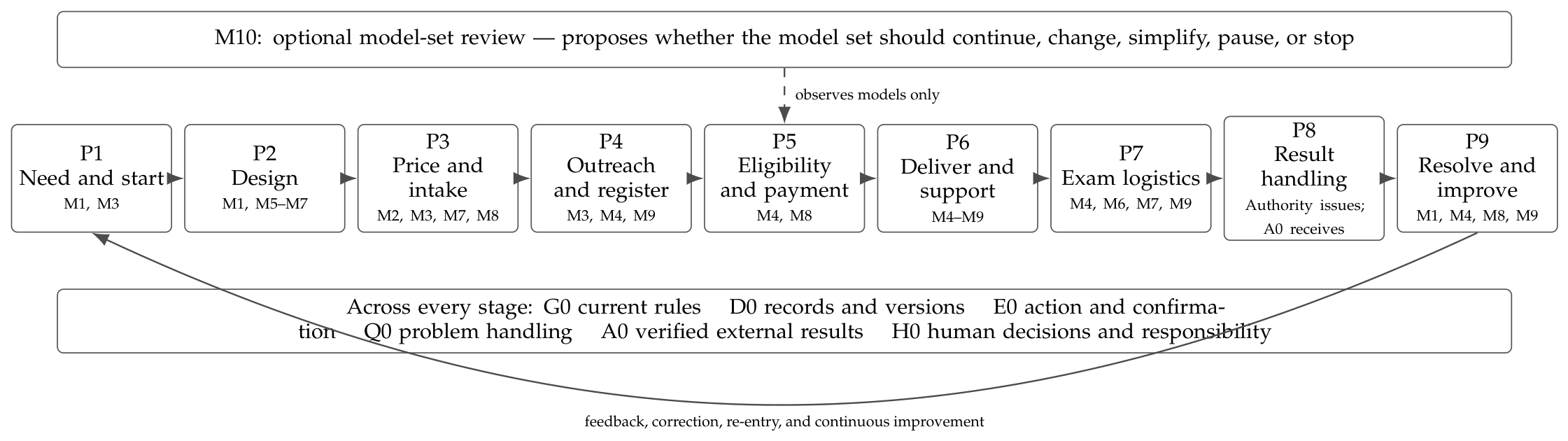
Table 1.
Closest integrative traditions in the literature examined and the remaining connection gap.
Table 1.
Closest integrative traditions in the literature examined and the remaining connection gap.
| Tradition | What it already connects | Remaining question | What this paper adds |
|---|---|---|---|
| Service blueprinting [27] | Learner-facing service, backstage work, and service evidence | How unlike operating decisions exchange information and close. | Named decisions, readiness checks, permitted actions, versioned hand-offs, and model exit. |
| Process mining [13] | Event records, observed paths, conformance, and process improvement | What should be defined before complete event logs exist. | A prospective design for authority, minimum inputs, allowed actions, and human fallback. |
| Human–AI and hybrid intelligence [28,29,30,31] | Human judgment, automation levels, interaction, and complementary work | How advice becomes a traceable operating result. | A chain that separates advice, approval, execution, confirmation, and later evidence. |
| Design science and FEDS [4,5,6] | Artifact construction and choices about when and how to assess a design | Which domain decisions and failure paths the artifact must connect. | Nine operating decisions, exceptional paths, and an optional model-set review. |
| Micro-credential and vocational-education research [32,33] | Institutional, learner, credential, and labor-market context | How to operate a program without confusing service and certification authority. | A route from program design to follow-up that keeps authoritative decisions outside the models. |
Table 2.
Design-conformance check for the candidate framework.
| Design requirement | Implemented response | Question for local use |
|---|---|---|
| Cover the service journey and exceptions | P1–P9 plus refund, complaint, appeal, correction, return, and feedback paths | Which local exception or return path is still missing? |
| Preserve authority | G0 and H0 keep operating advice and human responsibility visible; the authorized body owns examination and certification decisions, while A0 receives and records them | Who owns each decision in the organization using the method? |
| Preserve meaning across hand-offs | Version, unit, owner, approval and confirmation accompany business information | Which local record carries these fields? |
| Allow a model to decline | Four readiness states include not applicable and unidentifiable | What simpler rule or human route remains available? |
| Keep models optional | Every stage has a human/rule fallback; M10 can be removed | Which models are unnecessary in this setting? |
| Check normal and failure paths | Ten synthetic workflow scenarios | Which local scenarios deserve an additional walkthrough? |
| Review change over time | M10 separates proposal, approval, confirmation and applied effect | Is model-set review useful yet, or is a simple checklist enough? |
Table 3.
Four shared innovation mechanisms across M1–M9.
| Mechanism | Models | Change to the decision design | Workflow consequence and boundary |
|---|---|---|---|
| Decision-object clarification | M1, M3, M4 | Names the attribute, forecast event, or learner state and preserves that meaning in later hand-offs. | Downstream models receive a defined business object rather than an unexplained score; clearer meaning does not by itself prove prediction accuracy or state validity. |
| Required conditions before preference | M2, M5, M8 | Builds the feasible set from capacity, qualification, authorization, access, or quality before comparing price, score, or profit. | An attractive number cannot compensate for an inadmissible action; the method still depends on the institution setting the right conditions. |
| Realistic action-space reconstruction | M6, M7 | Adds legitimate alternatives such as no permanent site and temporary service, while separating physical items, expiring service time, and aging digital content. | The model compares actions that can exist in practice without adding unlike units; it cannot create capacity or service quality that is absent in reality. |
| Explicit abstention | M9 | Treats no action and no recommendation as defined outcomes when permission, support, stability, or value is insufficient. | Weak evidence returns the decision to rules or a responsible person instead of forcing an answer; abstention alone does not identify causal benefit. |
Table 4.
Where models may support the business journey.
| Node | Opening object/event | Decision and accountable boundary | Candidate | Close event and common return path |
|---|---|---|---|---|
| G0 | New or changed rule, authority, standard, or policy | Approve rule, owner, scope, effective date, and prohibited actions | No optimizer | Signed/versioned rule enters D0; unknown or conflicting rule returns to H0 and source authority. |
| P1 | New occupational/learner need or project proposal | Decide whether to initiate or revise an offering; no certification decision | M1; M3 as scenario support | Approved project brief or rejection; later P9 feedback returns to P1. |
| P2 | Approved need and design brief | Design curriculum, version, staffing, delivery mode, partners, and quality standard | M1, M5–M7 | Approved claims boundary, curriculum/content version, qualified instructor and replacement plan, and delivery/platform plan; capability failure returns to P1/G0. |
| P3 | Deliverable product and intake occasion | Set price, recruitment, channel, intake, and capacity envelope | M2, M3, M7, M8 | Approved price, recruitment, capacity, and cost plan with a validity window; overload or weak economics returns to P2/P3. |
| P4 | Campaign, consultation, trial, or registration event | Manage lawful outreach and state progression; no automatic enrollment entitlement | M3, M4, M9 conditionally | Approved claims/script used, consent and contact recorded, and registration accepted or declined; data or consent issue returns to G0/Q0/H0. |
| P5 | Application, document, order, payment, cancellation, or refund | Verify, request correction, transact, reconcile, or refund under rules | M4 and M8 as support only | Service eligibility, contract/order, payment, invoice, refund, and reconciliation status recorded; exception returns to applicant, finance, G0, or H0. |
| P6 | Valid enrollment and service-start event | Open access, schedule, allocate resources, support learning, assess progress, and manage content versions | M4–M9 as applicable | Learning and service result, formative assessment, make-up action or platform incident, and applicable content version recorded; shortage, weak learning outcome, or complaint returns to P2/P3/Q0. |
| P7 | Examination-application window | Training staff check document completeness and internal prerequisites; the authorized body makes any required final examination-eligibility decision and exceptions | M4, M6, M7, M9 as support only | Preliminary check, submission, authorized eligibility response, seat/date, notice, and exception status recorded; an internal deficiency returns to P5/P6, while an external decision is referred to the authorized body. |
| P8 | Result issued by an authorized body | Receive, authenticate, record, communicate, and support queries; do not decide, correct, or withdraw the authoritative result | No operating optimizer; M4 observes state | A0-verified external result linked to the training operator’s receipt and communication record; correction or withdrawal returns to the authorized body, while an appeal is forwarded through P9. |
| P9 | Lifecycle case resolution, follow-up service, and feedback | Resolve service complaints and financial disputes; forward and track certification appeals; support resit, maintenance, employment, and lawful aggregate learning | M1/M8 use closed-case aggregates; M4 observes state; M9 supports notices only | Accountable owner, disposition, notice, remedy, and execution confirmation recorded; the authorized body makes any certification disposition and A0 records its return; curriculum quality, occupational competence, and employer feedback return to P2. |
| Model review | Scheduled review, changed conditions, stale evidence, missing confirmation, or serious failure | Propose how the model set should be handled; no operational or certification authority | M10 optional | H0 decision + E0 confirmation + D0 adopted version; failure preserves the prior record and uses a human alternative. |
Table 5.
Minimum role map for the candidate workflow.
| Stage | Accountable | Responsible | Must be consulted or informed |
|---|---|---|---|
| P1–P2 | Program owner | Product/curriculum lead | Employer or learner representatives, teaching lead, rules/data lead |
| P3 | Program owner | Operations and finance | Recruitment, teaching support, partner manager |
| P4 | Recruitment owner | Consultation/channel team | Rules/data lead; prospective learner receives approved claims and terms |
| P5: eligibility/order | Operations or eligibility owner | Eligibility and order staff | Learner, finance, and rules lead |
| P5: payment/refund | Finance owner | Payment, invoice, refund, and reconciliation staff | Learner, operations, and case owner when disputed |
| P6 | Teaching-service owner | Instructor and learner-support team | Product, platform, scheduling, quality and data roles |
| P7: preliminary check | Examination-coordination owner | Examination-service team checks documents and internal prerequisites | Learner, training operations, authorized examination body |
| P7: final eligibility | Authorized examination body, when its rules require a final decision | Its designated eligibility staff | Learner and examination-liaison owner are informed |
| P8: authority | Authorized examination/certification body | Its designated examination/certification staff | Training operator and learner are informed; the operator does not decide the result |
| P8: internal handling | Examination-liaison owner | Result receipt, authentication, registration, communication, and query staff | Authorized body, learner, data/records lead |
| P9: service complaint | Service-quality owner | Complaint and service-recovery staff | Relevant stage owner, learner, and rules lead |
| P9: financial dispute | Finance owner | Finance case and reconciliation staff | Learner, operations, payment provider when needed |
| P9: appeal decision | Authorized body | Its designated appeal staff | Learner and examination-liaison owner are informed |
| P9: appeal tracking | Examination-liaison owner | Internal staff forward, record, notify, and follow up | Learner, authorized body, and records lead |
| Model review | Business/model-risk owner approves pause, change, or return | Data/algorithm and system teams implement the approved version | Independent reviewer confirms activation; rules lead and affected staff are informed |
Table 6.
The ten executable prototypes and the decisions they support.
| ID | Prototype name | Decision | Main change from a simple baseline |
|---|---|---|---|
| M1 | Rule-filtered Multi-role Greedy Selector (RMGS) | Product attributes | Removes disallowed attributes, protects the least satisfied role, and makes disagreement visible before greedy selection. |
| M2 | PSM-bounded Scenario Price Selector (PSPS) | Price and intake | Uses price perception only to set a search range; capacity and group differences are checked before profit. |
| M3 | Shock-augmented Bass Ridge Forecaster (SBRF) | Demand path | Names the predicted event and adds an observed shock term to a bounded Bass forecast. |
| M4 | Eligibility-conditioned Journey Transition Table (EJTT) | Learner journey | Conditions transitions on eligibility and removes impossible next states before probabilities are returned. |
| M5 | Qualified Partner Portfolio Enumerator (QPPE) | Partner combination | Excludes unqualified and fixed actors, then compares small partner combinations under scenarios. |
| M6 | Zero-site Hybrid Coverage Enumerator (ZHCE) | Service coverage | Compares online, permanent, and temporary service, including the choice to open no permanent point. |
| M7 | Three-class Quantile Resource Planner (TQRP) | Resource plan | Plans physical items, service hours, and digital updates separately instead of treating all three as inventory. |
| M8 | Feasibility-first Tail-profit Selector (FTPS) | Cohort economics | Removes actions that fail minimum conditions, then compares poor-case profit before average profit. |
| M9 | Stable Eligible Action Selector (SEAS) | Next action | Considers only allowed actions with sufficient and temporally stable evidence; otherwise makes no recommendation. |
| M10 | Evidence- and Reversibility-aware Model Review (ERMR) | Model-set review | Compares six review responses in a fixed order, including missing evidence and whether an earlier stable version really exists. |
Table 7.
Information required when the ten prototypes are connected to a workflow.
| ID | Minimum input | Main output | Next use |
|---|---|---|---|
| M1 | Product version, attributes, role scores, allowed flags, cost, budget | Selected and excluded attributes; disagreement information | Approved product version for M2/M3 |
| M2 | Product version, price grid, PSM range, demand/refund scenarios, cost, capacity, group-difference limit | Price, number of feasible prices, poor-case profit, or reason not to price | Approval; demand and resource planning in M3/M7/M8 |
| M3 | Named event, cumulative training series, market ceiling, observed shocks, future period | p, q, shock coefficient, bounded time path | Demand scenarios for M7/M8, never a direct staffing instruction |
| M4 | State definitions, eligibility, age group, observed transitions, prohibited moves | Next-state probabilities, a separate REVIEW_REQUIRED signal, service arrivals, or reason no estimate is possible | Workload for M7; reviewed cases for Q0 and suitable cases for M9 |
| M5 | Candidate identity, qualification, fixed-actor flag, scenario utility, capacity, cost | Partner combination and worst-scenario score | Partner-agreement approval; available capability for M6/M7/M8 |
| M6 | Regional demand, required on-site share, distances, site capacities/costs, temporary cost | Permanent-point choice, total cost, temporary-service share | Regional service capacity for M7 |
| M7 | Training demand for three resource classes and a digital-aging exposure score | Physical-requirement target, service capacity, digital update interval, or reduced plan | Feasibility information for M2/M8 |
| M8 | Candidate cohort actions, profit scenarios, minimum-condition status, quality scenarios | Cohort action, poor-case and mean profit, or no automated choice | Approval and execution; operating range for M9 |
| M9 | Context, allowed actions, eligible history, support and stability limits, action cost, no-action value | Context-specific action whose net value exceeds , its stability, or no recommendation | Risk-based approval and execution |
| M10 | Model-set version, model signals, missing results or confirmations, rule status, stable version, prior review | Review proposal, affected models, missing-evidence score, expected risk, decision status | Human decision, action confirmation, and adopted-version record |
Table 8.
Executable business-journey scenarios and observed terminal states.
| Scenario | Trigger | Rule checked | Outcome/path |
|---|---|---|---|
| Successful journey | No exception | Versioned hand-offs and confirmations exist through all stages | Completed; P1–P9 |
| Routine refund | Approved ordinary refund at P5 | A routine refund closes with its transaction record and need not become a P9 dispute | Refunded; closes at P5 |
| Refund dispute | Refund remains disputed at P5 | Financial disagreement receives a named P9 case owner | Dispute resolved; P5→P9 |
| Service complaint | Service problem arises at P6 | The service-quality path is separate from certification authority | Complaint resolved; P6→P9 |
| Certification appeal | Learner challenges a result after P8 | P9 forwards it, the authorized body returns its disposition through A0, and P9 links notice and closure | Closed; P8→P9→P8→P9 |
| Learning-quality return | P6 assessment signals weak learning quality | Service-quality owner records remedy and cause; approved feedback returns to P2 as a new program revision record | Improvement recorded; P6→P9→P2 |
| Service ineligibility | Service/admission condition fails at P5 | An ineligible record cannot enter learning service | Closed as ineligible; no P6 |
| Examination ineligibility | An operator-owned prerequisite fails or the authorized body issues an ineligible decision at P7 | Learning may occur, but the case cannot proceed to P8; the source of the decision is retained | Closed as exam-ineligible; no P8 |
| Missing critical confirmation | Required completion confirmation is absent at P6 | Only a confirmation defined as an examination prerequisite blocks P7 | Blocked; stops at P6 |
| Model not applicable | A candidate model declines at P3 | Human workflow and responsibility remain available without the model | Completed; P1–P9 |
Table 9.
What changed in the synthetic mechanism checks for M1–M9 (means over ten fixed seeds).
| ID | Primary measure (lower is better) | Comparator | Candidate | Interpretation and retained trade-off |
|---|---|---|---|---|
| M1 | Regret | 0.9475 | 0.1556 | Lower in 9/10 seeds; RMGS also removes disallowed choices, so the difference is not a pure gain in estimating Kano preferences. |
| M2 | Group registration-rate difference | 0.4370 | 0.2726 | Capacity violations fall from 0.0519 to 0, but mean synthetic profit falls from 408,913 to 186,380. This difference is only one signal for later fairness discussion. |
| M3 | Mean absolute path error (MAE) | 2.7507 | 2.6150 | Lower is better; only 5/10 seeds improve. The shock-aware form has no stable advantage in these worlds. |
| M4 | Prohibited-transition probability | 0.2414 | 0 | On EJTT’s shared non-review set, accuracy rises from 0.4975 to 0.5644, NLL changes from 1.1171 to 1.1375, and paid-count error from 8.01 to 11.85; 6.54% are routed to review. |
| M5 | Unqualified partner rate | 1 | 0 | The qualification check works by construction; worst utility rises from 0.052 to 2.295, but the two methods do not choose from the same set. |
| M6 | Total cost | 9,166.75 | 7,001.96 | Candidate opens no permanent site and uses 24.26% temporary service, but the regional gap worsens from 0.1276 to 0.2300, above the 0.18 soft reference. Result depends on unlimited temporary capacity and the stated penalty. |
| M7 | Total cost | 835.17 | 801.44 | Service overflow and accumulated digital-aging exposure fall, but physical shortage rises from 0 to 0.697. |
| M8 | Minimum-condition failures | 0.20 | 0 | Strictly better in 2/10 and no worse in 10/10 seeds. Mean profit falls from 145.23 to 129.72; poor-case mean rises from 72.49 to 101.59. |
| M9 | Disallowed action rate | 0 | 0 | Under shared permission and eligibility checks, both methods avoid disallowed actions. SEAS acts less often (0.7021 vs. 0.8007) and mean synthetic gain falls from 0.2463 to 0.2122. |
Disclaimer/Publisher’s Note: The statements, opinions and data contained in all publications are solely those of the individual author(s) and contributor(s) and not of MDPI and/or the editor(s). MDPI and/or the editor(s) disclaim responsibility for any injury to people or property resulting from any ideas, methods, instructions or products referred to in the content. |
© 2026 by the author. Licensee MDPI, Basel, Switzerland. This article is an open access article distributed under the terms and conditions of the Creative Commons Attribution (CC BY) license.
Copyright: This open access article is published under a Creative Commons CC BY 4.0 license, which permit the free download, distribution, and reuse, provided that the author and preprint are cited in any reuse.


