Climate Signal or Network Artefact? A Relative-Homogeneity and Gauge-Support Screen for Areal Precipitation Trends, Applied to 73 Greek Lake Catchments

Nikolaos Gourgouletis; Evangelos Baltas

doi:10.20944/preprints202608.0406.v1

Submitted:

04 August 2026

Posted:

06 August 2026

You are already at the latest version

Abstract

Areal precipitation series inherit their network’s composition: no record separates a station discontinuity from a regional shift; changing which gauges report moves the mean with none changing. The screen is two-layer, implementable on any network: a four-test relative-homogeneity battery on each gauge’s neighbour-ratio series, then propagation of those verdicts through realized rather than static Thiessen weights. Of Greece’s 187 weight-carrying gauges, 168 were testable and 19 were not; 96 classified useful, 30 doubtful and 42 suspect; relative and absolute verdicts agreed for only 87 of 168 (κ = 0.17). A drop-only screen cannot change a retained slope, so the suspect gauges are deleted, the weights renormalized over the survivors and every areal series rebuilt: of 16 field-significant increases, 14 survive, 2 lose field significance and 3 new detections appear on two distinct series. Individual catchment verdicts are fragile; the field verdict is not: it holds under nulls recalibrated for persistence, skewness and calendar gaps, and under every removal rule but the most aggressive, which leaves 10. That invariance is to detectable, non-shared inhomogeneity only. Deletion itself amplifies, 7 of 71 catchments rising to 16 of 66. Homogeneity screening alone is insufficient: the one field-significant decrease passes it yet is composition-dominated.

Keywords:

relative homogeneity

;

areal precipitation

;

gauge network composition

;

Thiessen weights

;

change-point detection

;

SNHT

;

Monte-Carlo critical values

;

trend attribution

;

Greece

Subject:

Environmental and Earth Sciences - Water Science and Technology

1. Introduction

A catchment precipitation series is almost never measured. It is constructed — by Thiessen polygons [1], inverse-distance weighting, kriging or a gridded interpolation — from point records that begin, end, move and change instrumentation on administrative rather than climatic schedules. The sparsity of that support is a well-documented global problem [2], and network design has long been treated as a first-order determinant of what a hydrometric record can support [3]. What is treated far less often is what happens to a derived areal series when the network changes during the record.

Whatever the interpolation, the constructed series carries two distinct kinds of non-climatic content. The first is familiar: a gauge record may contain a step change caused by relocation, a change of exposure, a change of gauge type or a change of observer, and that step propagates into the areal mean in proportion to the gauge’s weight. The second is less often confronted at catchment scale, although it is a known problem in the construction of large-area averages: the set of gauges contributing to a given year is not constant. When a weighting scheme renormalizes over the gauges that actually reported — as almost every operational implementation does, because the alternative is to discard the year — the effective weight of a surviving gauge rises as its neighbours terminate. If that gauge sits at a systematically different mean level from the ones it replaces, the areal series steps. And it steps without any gauge record containing a step at all.

Both mechanisms matter for trend detection, and neither is addressed by the statistical machinery trend studies normally apply. A Mann–Kendall test [4,5] with a Hamed–Rao variance correction [6] handles serial dependence — itself a consequential and contested choice [7,8]. A Benjamini–Hochberg procedure [9] handles multiplicity across a field of catchments, with Benjamini–Yekutieli [10] available when dependence cannot be signed, and field significance is by now an expectation rather than an option [11]. A Theil–Sen estimator [12] gives a robust slope. None of them asks whether the series being tested is a homogeneous measurement of anything. A field of trends can be internally impeccable and still be a map of the archive’s administrative history — a failure mode adjacent to, but distinct from, the methodological over-reading diagnosed elsewhere in the trend literature [13].

The homogenization literature is mature, and its central insight is old: homogeneity must be assessed relatively, against neighbouring records, because a candidate series tested against itself confounds station history with regional climate [14,15,16,17]. The standard normal homogeneity test (SNHT), the Buishand [18] range test, the Pettitt [19] rank test and the von Neumann [20] ratio form the conventional four-test battery, and the convention for combining them — 0–1 rejections useful, 2 doubtful, 3–4 suspect — was fixed for European daily series by Wijngaard et al. [21] and used to characterize the European Climate Assessment dataset [22]. Fully automated systems exist and have been benchmarked against one another on synthetic networks with known inhomogeneities [23,24,25,26], and national applications, including for Greek temperature, are established [27]. A distinct branch dispenses with a composite reference altogether and works from pairwise differences among all admissible neighbour pairs [28] — the direct alternative to the composite-reference construction used here, and one that shares its blindness to network composition, since a pairwise difference is still a statement about gauges. What the automated, interactive and pairwise families have in common is their objective and their yardstick: they exist to correct series, and they are judged on how faithfully they recover inhomogeneities that are known because they were inserted.

The stakes are not merely procedural. Whether Mediterranean precipitation is declining remains actively contested, with assessments reaching different conclusions depending on region, season and window [29,30], and with recent work arguing that high temporal variability rather than trend dominates the regional signal [31]. In a debate of that kind, a gauge-network artefact of a few tens of millimetres per decade in a subset of catchments is not a rounding error. It is the size of the effect being argued about.

Three gaps separate that literature from the problem a catchment-scale trend study actually faces. The first is one of purpose. Homogenization is normally an end in itself: the deliverable is a corrected series or a corrected gridded product. A trend study that inherits a network it did not build, and that reports an uncorrected estimate because a corrected product would be a different deliverable — one requiring its own validation and a strongly method-dependent choice of correction package (Section 4.5) — needs something else. It needs a screen that says how much of a given catchment’s areal estimate rests on questionable support, and whether the study’s conclusions survive removing that support. The relevant unit is not the gauge but the catchment-year weight.

The second gap is not the machinery. Two of the four tests used here were introduced on rainfall records in the first place [14,18], ACMANT has a precipitation branch [26], the MULTITEST project benchmarked packages on synthetic monthly precipitation alongside temperature [32], and four packages have been compared on 299 Irish precipitation records [33]. The gap sits upstream of the test statistic. Precipitation is harder than temperature because annual totals at two stations 15 km apart in complex terrain routinely correlate below the thresholds temperature homogenization takes for granted, so the reference-construction step is where a precipitation application succeeds or fails. What is scarce is not a test but a reference-admission rule: a reproducible statement of what counts as a usable precipitation reference, published with its failure mode and with the gauges it excludes counted as their own class rather than quietly passed.

The third gap matters most here. The network-composition mechanism described above is documented — but in a different literature, and answered there in a way a catchment-scale trend study cannot simply inherit. Wherever a large-area average is assembled from a station population that changes over time, the standard structural response is to combine anomalies rather than absolute values: the reference-station, climate-anomaly and first-difference methods were devised precisely so that a change in which stations report does not move the average [34], and operational gridded products interpolate monthly anomalies for the same reason [35]. A relative battery cannot see the mechanism at all, because it is not a property of any gauge: every record can pass every relative test while the areal series still contains a composition-driven step. What appears to be missing from both literatures is the diagnostic a study inheriting a published areal product actually needs — a per-catchment, per-year statement of how much of an areal estimate rests on questionable support, and of whether the conclusions survive removing it. Homogeneity screening and gauge-support screening answer different questions, and a study that runs only the first will confidently certify an artefact.

The absence of an integrated screen has a quieter consequence as well. Change-point evidence is often produced by applying an absolute test — commonly Pettitt — to the areal or gauge series and reporting the resulting break years, and such evidence is easy to over-read. A regional wet-to-dry transition and a network-wide instrumentation programme both produce clusters of absolute break years; only a relative test can tell which is which. Section 3.4 shows that on the same 168 series the absolute and relative verdicts agree for barely half the gauges.

This paper therefore sets out a two-layer screen and applies it to a real, awkward network. The contribution is method, not a regional climate claim, and it has five parts.

A reproducible relative-homogeneity battery for precipitation, with an explicitly stated neighbour-admission rule, a composite reference whose correlation with the candidate is itself gated, four test statistics with Monte-Carlo rather than tabulated critical values, and a unit-test suite that verifies the size, power and break-location behaviour of every implementation before any result is produced.
A fail-closed reconstruction proof that certifies the screen is screening the right gauges. Gauge series rebuilt from raw daily files, recombined with the published areal weights, must reproduce the published areal series catchment by catchment and year by year within an analytic bound, or the procedure aborts. Without it, a homogeneity assessment of “the network” is an assessment of a set of gauges that may not be the set the areal product used.
Propagation through realized rather than static weights, which is what makes the screen quantitative at catchment scale, and which exposes the composition mechanism as a by-product.
A leave-suspect-out reconstruction, the operation that makes the screen a test rather than a subset. A drop-only screen leaves every retained series bit-identical, so its count of catchments that are retained and then lose field significance is close to structurally guaranteed to be zero. Deleting the suspect gauges, renormalizing the weights over the survivors and rebuilding the areal series can and does change verdicts; the changes are reported here, including those that count against the screen.
A result reported with its failures, together with the diagnostics that distinguish “the screen removed the signal” from “the screen removed catchments”, and an explicit statement of what the screen cannot do.

Section 2 sets out the data, states the method in transferable form and gives the parameter values used for the Greek application. Section 3 reports the results, Section 4 discusses them and states the limits, and Section 5 concludes.

2. Materials and Methods

2.1. Data

2.1.1. The Gauge Archive

The input is the Greek national daily-rainfall archive as exposed through the Hydroscope national databank [36] together with the national meteorological service’s daily series. From the full inventory, candidate series were those that are daily, of the rainfall variable group, carry coordinates, pass a record-length pre-filter, and — for the meteorological-service subset — are reported in millimetres and are not duration series. This yields 466 candidate daily-rainfall series.

Three successive filters, applied in a fixed order, reduce the candidates to the gauge universe: a value-based completeness filter requiring at least ten years with at least 340 real daily values each (drops 101); a record-quality filter on the meteorological-service subset requiring at least 25 valid years, a mean annual total between 150 and 2,500 mm, and a first valid year no later than 1990 (drops 25); and a co-located de-duplication on rounded projected coordinates, retaining the series with the most valid years (drops 0 here). The result is a gauge universe of 340 gauges (Table 1).

Annual totals are calendar-year sums over years with at least 340 real daily values; a plausibility floor masks annual totals below 30 mm, affecting 25 gauge-years. A second, season-level floor masks a gauge-season whose recorded days pass the seasonal coverage rule but whose total is exactly zero — the signature of a zero-filled rather than a dry season, which an annual-only floor cannot see because the remaining months carry the annual total above 30 mm — and propagates that mask to the gauge’s annual value as the first floor does; it removes 57 further gauge-years. The resulting annual matrix spans 1932–2019 and holds 86 of those 88 calendar years by 340 gauges — no gauge anywhere in the network meets the 340-real-day rule in 1944 or 1945, so those two wartime years carry no valid gauge-year and are absent — with 15,602 valid gauge-years.

2.1.2. Catchments and Their Weights

Seventy-three lake catchments are delineated across the fourteen Greek river-basin districts, and each has a Thiessen weight vector over the gauge universe. 187 of the 340 gauges carry non-zero Thiessen weight and are therefore the gauges whose homogeneity can affect a published areal series; these 187 are the population screened here. Six of the 187 come from the meteorological-service subset; among the 187 the median full-record length is 51 years and the median length inside the 1984–2019 analysis window is 29 years. Catchments carry between 1 and 27 weighted gauges (median 3); 21 of the 73 are single-gauge catchments.

One duplicate pair was detected among the annual series — two archive entries under the name ΚAΣΤEΛΙ, identical over 34 common years — and each was excluded from the other’s reference set, because a candidate referenced against a copy of itself cannot be tested.

2.1.3. The Trend Family Being Screened

The areal precipitation series screened in Section 3 are Thiessen-weighted annual catchment totals over the 73 lake catchments, built from the daily gauge records of Section 2.1.1 — the Hydroscope national daily-rainfall archive together with the national meteorological service’s daily series — using the catchment weight vectors of Section 2.1.2. Those series, those weights and the catchment trend family estimated from them are the ones reported by a companion catchment-scale hydroclimatic analysis by the present authors (manuscript in preparation). The weights are not provider metadata but the authors’ own derived product: the 73 catchments were delineated from the 25 m EU-DEM digital elevation model [37] by flow-direction and flow-accumulation procedures from each lake outlet, and each gauge’s Thiessen (Voronoi) weight is the area fraction of the catchment nearest that gauge on a 1 km grid, renormalized each year over the gauges that actually reported — the realized weighting whose consequences Section 2.2.6 propagates. The derived series and the trend family are deposited, and the deposit is named under Data availability; the gauge-to-catchment weight table is not, because it is keyed one-to-one to a station inventory of names and coordinates, although a reader holding the public gauge coordinates can recompute it and the five weights of the EL13 Aposelemi catchment are printed in Section 3.7. The screened quantity is the annual precipitation trend field over 1984–2019, the openly disseminated daily record ending in 2019, estimated with a Theil–Sen slope and a modified Mann–Kendall test with an ungated lag-1 Hamed–Rao variance inflation, and controlled for multiplicity by Benjamini–Hochberg at q = 0.05 within each family. The unscreened family comprises 71 catchments (two of the 73 fall below the minimum-length requirement), with 30 raw-significant increases and 1 raw-significant decrease, 16 increases and 1 decrease surviving false-discovery-rate control, and a network-median slope of +54.222 mm decade⁻¹. These values are reproduced by the screening code as a parity gate (Section 2.2.6) before any screened variant is computed. The present paper does not defend or reinterpret that field; it screens it. Those Benjamini–Hochberg counts are adopted under positive regression dependence on a subset (PRDS), a property this spatially correlated field is assumed rather than shown to have: under the arbitrary-dependence Benjamini–Yekutieli variant, whose penalty here is c(71) = 4.85, just one of the 16 increases survives in this family — EL04_LIMNI_EVINOU, at p = 1.30 × 10⁻⁴ against a rank-one threshold of 1.45 × 10⁻⁴ — and the decrease does not, so every count screened below is a Benjamini–Hochberg count conditional on that assumption.

2.2. The Two-Layer Screen

The method is stated here in general terms. Everything in this section is independent of Greece and of the particular trend estimator; a reader with another network, another weighting scheme and another trend test can implement it as written. Section 2.3 gives the parameter values used in the present application.

2.2.1. Step 0: Reconstruct, and Prove the Reconstruction

The screen begins with an operation that is usually skipped. Rebuild the gauge-level series from the raw inputs using the areal product’s own construction rules — the same completeness thresholds, the same plausibility masks, the same de-duplication — then recombine them with the published weights under the product’s own missing-data policy, and require that the result reproduce the published areal series.

Two things must match: the year set of every catchment, which encodes the gauge-availability structure and is therefore the object the second screening layer reasons about; and the values, to within an analytic bound derived from the precision at which the weights are stored. If weights are stored rounded to d decimals, each weight deviates by at most 5 × 10⁻⁽ᵈ⁺¹⁾ from its exact value, and the induced deviation of a catchment-year value is bounded by

|ΔP| ≤ (5 × 10⁻⁽ᵈ⁺¹⁾ / Σ_i w_i r_i) · Σ_i r_i |x_i − P| + δ_print,

where x_i is gauge i’s value, r_i indicates whether it reported, P is the areal value and δ_print is the rounding at which the product is published. Any catchment-year exceeding its own bound is a genuine disagreement and must halt the procedure.

This step is not bookkeeping. Without it, a homogeneity assessment is an assessment of a set of gauges, and the inference that a given catchment’s areal estimate rests on suspect support is unsupported. With it, the gauges screened are provably the gauges the areal series is built from.

2.2.2. Step 1: A Composite Reference for Each Candidate

For each candidate gauge, admissible neighbours are those that (i) lie within a maximum distance, (ii) share at least a minimum number of valid years with the candidate over the full record, (iii) correlate with the candidate above an individual-correlation floor, and (iv) are not duplicates of the candidate.

The reference is an Alexandersson-type composite: each admitted neighbour is rescaled to the candidate’s mean over their common years and the rescaled neighbours are averaged with weights r², where r is the neighbour’s correlation with the candidate. A reference value exists for a year when at least two neighbours report it.

Neighbour selection proceeds in tiers. The primary tier takes the k nearest admissible neighbours. If the resulting composite fails the reference gate, the k best-correlated admissible neighbours are tried. If neither in-window tier yields an admissible reference — for any of the gate’s reasons, whether the candidate or the reference is too short inside the analysis window or the in-window composite simply fails the correlation criterion — both tiers are retried on the full record. The tier and the window actually used are recorded for every gauge, and both belong in the result: a gauge recovered on its full record is classified over a longer span than the trend field being screened, which is a real if unavoidable mismatch.

The reference gate is where a precipitation application succeeds or fails. A usable reference requires at least three neighbours, at least a minimum number of test years, and — the operative criterion — a Pearson correlation between candidate and composite above a threshold. For annual precipitation totals in mountainous terrain, single-gauge correlations rarely reach the level at which a difference or ratio series is informative even at short separations, whereas a five-gauge composite generally does. Gating on the composite correlation rather than on individual neighbour correlations is therefore the design decision that makes the battery usable for precipitation.

A gauge that fails the gate is recorded as untestable, with the reason. It is emphatically not recorded as useful. Treating “no usable reference” as “passed” is the single most consequential error available in this analysis, because the gauges without references are systematically the isolated and insular ones — exactly the ones whose weight a sparse network concentrates.

2.2.3. Step 2: The Test Series

Two test series are formed per gauge over the years where both candidate and reference exist:

the ratio series x_i / ρ_i (primary; the multiplicative convention appropriate to precipitation), and
the difference series x_i − ρ_i (reported alongside).

The candidate’s own absolute series is deliberately not tested. That is the entire point of the design: a regional climatic shift is common to candidate and reference and cancels in the ratio, whereas a station-specific discontinuity does not. Section 3.4 shows what is lost by testing the absolute series instead.

2.2.4. Step 3: Four Tests with Simulated Critical Values

The four conventional tests are applied to each test series (Table 2). SNHT [14] maximizes a two-segment likelihood-ratio statistic on the standardized series; the Buishand [18] range test uses the rescaled adjusted partial-sum range; Pettitt [19] uses the rank-based Mann–Whitney statistic maximized over split points; the von Neumann [20] ratio compares the mean square successive difference with the variance and, unlike the others, does not locate a break — it detects departure from randomness in either direction and is rejected in the lower tail.

Critical values and p-values are obtained by Monte-Carlo simulation under an i.i.d. Gaussian null, separately for every series length present in the dataset, from a generator seeded deterministically as a function of the length. There are three reasons to simulate rather than to transcribe published tables. Tabulated values exist only at selected lengths and interpolating between them is an uncontrolled approximation; the published tables differ in their normalization conventions (the Buishand statistic in particular is reported both as R and as R/√n, and with the standard deviation defined with either n or n − 1 in the denominator), so a transcription error is silent; and simulation makes every critical value auditable and exactly reproducible from a seed. An upper-tail p-value is computed with the add-one estimator, which never returns exactly zero. Simulated sizes and error rates are quoted in the text to the precision their replicate counts support (at 50,000 replicates the binomial standard error of a rate near 0.02 is about 0.0006); the per-quantity Monte-Carlo standard errors are carried in the archived gate reports and per-gauge tables beside the estimates rather than repeated inline. The null is Gaussian while the tested quantity is a ratio of two right-skewed variables; Section 4.5 and Table 3 measure what that costs, and the answer is that the individual tests are mis-sized but the three-of-four rule is not.

The von Neumann statistic provides an independent correctness check on the simulation, because its null moments are known analytically: E[N] = 2 and Var[N] = 4(n − 2)/(n² − 1). Agreement between the simulated and analytic moments verifies the null-generation machinery without reference to any published table.

Each gauge is classified on the number of tests rejecting at the 5% level, following the convention of Wijngaard et al. [21]: 0–1 useful, 2 doubtful, 3–4 suspect.

2.2.5. Step 4: Implementation Unit Tests, Run Before Results

The battery is only as trustworthy as its four implementations, and all four are easy to get subtly wrong. Before any substantive result is produced, the following are verified, and a failure aborts the run:

Size. On homogeneous i.i.d. series of length 36 — the width of the analysis window, against a modal primary test-series length of 32 and a median of 30 — each test’s rejection rate at the nominal 5% level must be ≈ 0.05.
Power. With a step of 1.5 standard deviations injected at the midpoint, each test’s rejection rate must exceed a stated floor.
Break location. For the three tests that locate a break, the median located split point must recover the injected one.
Noiseless discontinuity. On a noiseless step, all four tests must reject and all three locating tests must return the correct year.
Noiseless control. On a single homogeneous realization, the classification must be useful.
Analytic moments. The simulated von Neumann null mean and variance must match theory.
Cross-implementation parity. The fast rank-identity Pettitt statistic must agree with an independent reference implementation, on both the break index and, where recoverable, the statistic itself.

A double-mass diagnostic is computed alongside as an interpretive aid: cumulative candidate against cumulative reference, with an objective two-segment least-squares break (minimum segment length imposed), reported as the break year, the post/pre slope ratio, the fractional sum-of-squares reduction and a nested-model F. The F is descriptive, not a calibrated test — cumulative series are serially dependent by construction — but the sign of the slope ratio is informative and is used in Section 3.5.

2.2.6. Step 5: Propagation to Catchments Through Realized Weights

The gauge verdicts are mapped into catchment space through the weights, and here the screen departs from what is usually done.

The published weight of a gauge is a static area share. The areal series, however, renormalizes each year over the gauges that actually reported. A gauge’s realized weight — the per-year renormalized share, averaged over the analysis window — is therefore the fraction of the areal estimate it actually produced, and it can differ from the static weight by more than an order of magnitude in either direction. A gauge with a large static weight but a short record contributes far less than its weight suggests; a nominally negligible gauge that outlives its neighbours contributes far more.

Each catchment therefore receives a weight fraction in each class — useful, doubtful, suspect, untestable — computed on realized weights (primary) and on static weights (reported as a sensitivity). Catchment-level screening scenarios then drop catchments whose class fraction exceeds a threshold, and the trend field is re-estimated on the retained subset with the multiplicity correction re-applied within the reduced family, since the family has changed.

Two design requirements make the re-runs interpretable:

Fail-closed parity. The unscreened family must be reproduced exactly — same n, same raw and adjusted counts, same median slope — before any screened variant is computed. Any discrepancy means the screening code and the published analysis are not the same analysis, and the comparison would be meaningless.
A scenario family, not a scenario. A single threshold is a researcher degree of freedom, so the screen is run over a grid of scenarios × thresholds spanning the plausible range of conservatism, from “drop any catchment with any suspect weight” to “tolerate half”.

2.2.7. Step 6: Leave-Suspect-Out Reconstruction

Catchment-level screening has a structural limitation that must be stated before its results are read, because it is easy to mistake for a finding.

A drop-only screen cannot change a retained catchment’s answer. Every retained catchment keeps the areal series it always had, so its Theil–Sen slope and its test statistic are bit-identical to the unscreened ones, and the only route to a changed verdict is the multiplicity correction, whose threshold depends on the size and composition of the family. A tally of “catchments retained by the screen that then lost field significance” is therefore close to structurally guaranteed to be small, and at a suspect-weight threshold of zero it is guaranteed to be uninformative, because the retained set carries no suspect weight by definition. Such a screen answers “is the conclusion carried by the clean part of the network?”, which is worth knowing, but not “does removing the questionable data change the answer?”.

The leave-suspect-out reconstruction answers the second question. For each catchment, delete the gauges its own classification flags, renormalize the weights over the survivors under the areal product’s own per-year missing-data policy, rebuild the areal annual series from the gauge series, and re-estimate the trend with the same estimator and the same multiplicity control. Reconstruction is used throughout in exactly this sense — re-aggregation of the areal series from the retained gauges under renormalized weights; no missing gauge value is infilled or estimated. The catchment set is held fixed as far as the data allow, so a change in a verdict is caused by the removal of the gauges and not by the shrinking of the family. A reversal, throughout this paper, is exactly that change of verdict — a catchment that held Benjamini–Hochberg field significance against the matched baseline and no longer holds it once its flagged gauges are deleted — and never a change in the sign of its slope; a change in the other direction, a catchment that gains field significance, is reported separately as a new detection. Three points of discipline make the comparison honest:

Compare reconstruction with reconstruction. The baseline is not the published series but the drop-nothing reconstruction, run through the identical pipeline. Any residual deviation from the published product — here, the effect of storing weights rounded to four decimals, which moves no drop-nothing slope by more than 0.091 mm decade⁻¹ — is then identical on the two sides for every catchment whose gauge set is unchanged, and of the same negligible order for those whose gauge set changes, so it cannot manufacture or mask a reversal.
Re-apply multiplicity control on the matched set. Because some catchments become unreconstructible, the baseline for the false-discovery-rate comparison is the drop-nothing reconstruction restricted to exactly the catchments that survive in that variant, with the correction re-applied. Otherwise a change in family size masquerades as a change in evidence.
Report the catchments that lose all support. A catchment whose every gauge is flagged has no reconstruction at all. That is an outcome, not a missing value, and it must be counted and named rather than silently dropped.

The same variant logic is applied to the gauge-removal rule, so the answer is reported as a range across variants rather than asserted from a single choice.

2.2.8. Step 7: Separating “Removed the Signal” from “Removed the Catchments”

Screened counts alone cannot answer the question. Dropping catchments shrinks the family, and a smaller family has less power under false-discovery-rate control, so a fall in the number of significant trends is expected even if screening changes nothing. Four diagnostics separate the explanations:

The rate, not the count. The proportion of retained catchments that are raw-significant is not mechanically reduced by shrinking the family. If inhomogeneity manufactured the trends, removing suspect catchments should lower this rate.
Dose–response. If inhomogeneity inflated the trends, suspect-heavy catchments should carry the larger slopes; a rank correlation between suspect weight fraction and slope should be strongly positive.
Sign symmetry. A network-wide artefact — a re-siting programme, a change of standard gauge — should be predominantly one-signed. Bidirectional relative breaks are the signature of station-specific noise rather than a coherent bias.
Reversal count under reconstruction. The decisive quantity, measured on rebuilt series rather than on a retained subset (Section 2.2.7): how many catchments keep a series after their suspect gauges are removed and then lose significance relative to the matched baseline. A reversal here is a changed Benjamini–Hochberg verdict caused by deleting data, in the sense defined in Section 2.2.7; the corresponding count from a drop-only screen is not.

2.3. Application to the Greek Network

2.3.1. Parameter Values

Neighbours: maximum distance 150 km; minimum 15 overlapping valid years; individual correlation floor r ≥ 0.50; k = 5 (with k = 3 as a sensitivity). Reference gate: at least 3 neighbours, at least 20 test years, and candidate-versus-composite correlation r ≥ 0.70. Test window 1984–2019, matching the analysis window of the trend family.

Monte-Carlo: 20,000 i.i.d. standard-normal replicates per series length, generator seeded as 20260725 + 1000n, giving deterministic critical values on the grid of 31 series lengths the run requested, n = 20 to n = 67. That grid is wider than the tested set: the 168 series actually tested span 21 to 67 years over 26 distinct lengths, while n = 20 — the reference gate’s minimum test-year count — and the n = 36 unit-test length are on the grid but carried by no tested series. 4,000 replicates per unit-test scenario. Classification threshold α = 0.05 throughout.

Catchment-level screening: six scenarios (A–F, Table 4) at three thresholds each (0.00, 0.25, 0.50), giving 18 combinations. Scenario A (realized suspect weight) is primary; B adds untestable weight to suspect, extending the range on the conservative side; C adds doubtful weight, which is deliberately over-conservative; D classifies on the worse of the ratio and difference verdicts; E counts a suspect gauge only if a located break falls inside the analysis window; F repeats A on static rather than realized weights.

Leave-suspect-out reconstruction (Section 2.2.7): seven gauge-removal rules (L1–L7), each applied to every catchment. L1 (delete every gauge classified suspect on the primary ratio series) is primary; L2 additionally deletes untestable gauges; L3 additionally deletes doubtful ones; L4 uses the worse of the ratio and difference verdicts; L5 deletes a suspect gauge only if its located break falls inside the analysis window; L6 and L7 use the multiplicity-controlled classifications of Section 3.2. A reconstructed catchment enters the family under the same minimum-length rule as the unscreened one (at least ten valid annual values in the window).

2.3.2. The Reconstruction Proof

The rebuilt gauge series recombined with the published Thiessen weights reproduced the published areal annual series for all 73 catchments over 4,287 catchment-years, with identical year sets in every catchment and every value inside its analytic weight-rounding bound (99.49% of catchment-years within 0.1 mm; the largest single deviation was 1.800 mm, in EL05_POURNARI2, a catchment with many gauges whose 4-decimal stored weights leave the widest bound). The gauges screened below are therefore provably the gauges the areal series is built from.

2.3.3. Testability of the Network

Of the 187 weight-carrying gauges, 168 obtained a usable reference and 19 did not (Table 1, Figure 1). Among the tested gauges the primary tier — the five nearest admissible neighbours inside the analysis window — sufficed for 115; 17 required the best-correlated five, and 36 fell through to the full record (27 nearest-five, 9 best-correlated-five). Those 36 divide into two unequal groups, and the distinction matters: 23 had fewer than the required 20 years in which candidate and composite both existed inside the window, while 13 had 23 to 35 window years, reached the correlation criterion in-window and simply failed it — against the 0.733 to 0.902 their full-record composites reached. Those 13 are therefore classified on 23 to 67 years of record, in most cases longer than the 36 the trend field they screen spans, and they are not a benign subset: 8 classify useful, 1 doubtful and 4 suspect. Test-series length ranged from 21 to 67 years (median 30). The candidate-versus-composite correlation ranged from 0.700 (the gate) to 0.960, with median 0.807, achieved at a median mean neighbour distance of 23.6 km from a median of 34 admissible neighbours.

The 19 untestable gauges failed for four reasons: too few admissible neighbours (9), reference correlation below 0.70 (6), too short a record (3), and — for one Cretan gauge with many neighbours but a composite covering only 18 of its 34 years — fewer than the 20 test years the battery requires (1). They are not a random sample. Five are island gauges — Naxos, Rhodes, two on Lesvos, and one on Crete — and the remainder are isolated mainland sites, several in the northern border mountains, where the surrounding archive is thin or the neighbours are decorrelated by terrain.

2.3.4. Declaration of Generative-AI Use

Generative-AI assistance was used in preparing this study — for data extraction, figure generation through writing and reviewing the figure-plotting code, and review of the existing analysis code, with every output reviewed and edited by the authors — and the tools, their versions, the period of use and the authors’ assumption of full responsibility for the content are stated in the Use of Generative AI declaration in the back matter.

3. Results

3.1. Classification of the Gauge Network

On the primary ratio series, the 168 testable gauges classify as 96 useful, 30 doubtful and 42 suspect (Figure 1, Table 1).

Three comparisons bear on how firm that classification is, and all three are reported on the same footing — raw agreement, the agreement expected by chance from the marginals, and Cohen’s κ — because reading one comparison as “stable” and another as “disagreement” when both are bare percentages is a double standard rather than an inference. The difference series gives 95 / 28 / 45 and agrees with the ratio verdict for 141 of 168 gauges (84%; chance 42%, κ = 0.72); taking the worse of the two per gauge gives 86 / 33 / 49. The k = 3 sensitivity, computable for 146 of the tested gauges, agrees for 102 (70%; chance 43%, κ = 0.47) and returns almost the same suspect count (37 at k = 3 against 36 at k = 5 on that same 146-gauge subset). The absolute battery of Section 3.4 agrees for 87 of 168 (52%; chance 42%, κ = 0.17).

The ordering is the point: substantial agreement between ratio and difference, moderate between k = 5 and k = 3, and barely distinguishable from chance between relative and absolute. The marginal totals are therefore robust to the design choices internal to the relative battery while the per-gauge labels are only moderately so — which is why the worst-of-two and k-sensitivity views are carried as screening scenarios rather than adopted as primary, and why per-gauge labels are never used here to make a claim about an individual station.

All four unit tests of size returned empirical rejection rates in the range 0.046–0.054 against the nominal 5%; power against an injected 1.5-standard-deviation step was 0.94 (SNHT), 0.93 (Buishand), 0.97 (Pettitt) and 0.68 (von Neumann); the three locating tests recovered the injected split point exactly at the median; the noiseless step was detected by all four with the correct year; and the simulated von Neumann null moments matched theory (mean 2.0016 against 2, variance 0.1034 against 0.1050). The fast Pettitt implementation agreed with the reference implementation on the break index in 200 of 200 random series and on the statistic in all 141 cases where it was recoverable (Table 2).

Figure 2 shows the two ends of the classification. AΝΩ BΡOΝΤOΥ (suspect; all four tests reject; n = 34 years, reference correlation 0.771) steps in its ratio to its neighbours from a segment mean of 0.84 to 1.28 at 1998, and its double-mass slope ratio is 1.366 — the gauge began recording about a third more, relative to its neighbours, than it had before. On this gauge the absolute battery agrees with the relative one, rejecting all four tests and locating the same break year, so AΝΩ BΡOΝΤOΥ is an illustration of a detected relative break and not of the divergence between the two designs. ΠΛAΤAΝOΣ (useful; no test rejects; n = 32, reference correlation 0.919) tracks its composite closely throughout, with a double-mass slope ratio of 0.968 — and is where the two designs do part company, since the absolute battery rejects two of its four tests and would call it doubtful. Neither gauge settles the comparison on its own; that is what Section 3.4 does, over all 168, where the two verdicts agree for barely half the network at κ = 0.17.

3.2. Multiplicity, and the Size of the Battery Under Serial Dependence

A paper whose complaint is that trend fields need multiplicity control cannot apply 672 uncorrected tests — 168 gauges × 4 statistics at α = 0.05 — and decline to examine the consequence. Both the inferential argument and the correction are therefore reported.

Why screening is a different inferential setting. Field significance controls the rate of false discoveries in a set of claims, and the claim there is “this catchment has a trend”. Nothing of that kind is claimed per gauge here. The class labels are not discoveries; they are the input to a removal rule whose purpose is to be over-inclusive, because the cost of retaining a broken gauge is a corrupted areal series while the cost of removing a sound one is a slightly thinner network. Multiplicity control moves in exactly the wrong direction for that purpose: it reduces the flagged set, and hence weakens the screen. Uncorrected testing is therefore the conservative choice for a screen, in the same way that it would be the anti-conservative choice for a set of discoveries.

The correction, applied. That argument does not excuse leaving the magnitude unmeasured, so it is computed here. Applying Benjamini–Hochberg at q = 0.05 within each test across the 168 gauges reduces the rejections from 62 to 31 (SNHT), 61 to 29 (Buishand), 49 to 23 (Pettitt) and 74 to 55 (von Neumann); applying it jointly across all 672 gauge-tests gives 31 / 30 / 24 / 47. Re-running the Wijngaard rule on the controlled rejections reclassifies the network as 133 useful, 14 doubtful and 21 suspect (within-test control) or 133 / 15 / 20 (joint control), against 96 / 30 / 42 uncorrected.

The controlled suspect set is a strict subset of the uncorrected one: all 21 were already suspect, and no gauge is promoted into the class by the correction. Both controlled classifications are carried through the leave-suspect-out reconstruction as variants L6 and L7 (Section 3.6), where they give the same two reversals as the uncorrected classification. The screen’s conclusion is therefore insensitive to the multiplicity choice, and the uncorrected classification is reported as primary on the stated grounds rather than because it is more favourable — it is not: it removes 42 gauges rather than 21. Two caveats attach to the correction rather than to the primary layer. Benjamini–Hochberg is applied here across 168 gauges within a test and across all 672 gauge-tests jointly, and neither family is shown to satisfy the dependence conditions the procedure requires — the four statistics are computed on the same series and neighbouring candidates share reference gauges — so the positive-regression-dependence assumption stated for the 71-catchment trend family in Section 2.1.3 is not claimed for either gauge-level family here. And the p-values corrected are the i.i.d.-calibrated ones whose size is measured below, so L6 and L7 are the multiplicity-controlled classifications of an i.i.d.-calibrated battery and not error-rate-controlled statements about station history.

The i.i.d. null is false for the whole battery, not for von Neumann alone. Von Neumann rejects for 74 of 168 gauges (44%), far above the other three (62, 61, 49), but all four counts stand far above the eight or nine that a correctly sized 5% test would return, and none of the four is distribution-free with respect to serial dependence, so one violation of the null mis-sizes all four. Simulating homogeneous AR(1) series at the median test-series length (n = 30) with the median lag-1 coefficient the ratio series actually show (+0.211, quantified below), and judging them against the same i.i.d. Monte-Carlo critical values the battery uses, the empirical size at a nominal 5% is 0.135 (SNHT), 0.164 (Buishand), 0.130 (Pettitt) and 0.282 (von Neumann) — inflation factors of 2.7, 3.3, 2.6 and 5.6. With the persistence removed the same code returns 0.051, 0.051, 0.049 and 0.050, and re-simulating the null as AR(1) at the same coefficient restores 0.053, 0.053, 0.050 and 0.053, so the over-rejection is a property of the null and not of the implementations. It worsens steeply: at φ = 0.4 the factors are 5.5, 7.0, 5.1 and 13.1.

The size of the rule is not the size of its tests. Those are marginal sizes, and because the four statistics are computed on the same series they are strongly dependent, so the size of the classification rule cannot be read off them and has to be simulated in its own right. Simulating the Wijngaard rule itself at n = 30 on 50,000 replicates, the probability that a homogeneous series is classified suspect — three or four rejections — is 0.020 under the i.i.d. null and 0.091 at the observed median persistence of φ = 0.211, rising to 0.239 at φ = 0.4; at φ = 0.227 it is 0.101, which is where two independent re-implementations of this calculation by the authors landed.

Four independent 5% tests would give 0.0005, so even at φ = 0 the rule is forty times the size that independence implies, and the whole of that excess is test dependence. In expectation this is 3.4 false suspects among 168 correctly calibrated gauges against 15.4 at the network’s observed persistence and 40.2 at φ = 0.4 — 168 × 0.0203, 0.0914 and 0.2395, the unrounded simulated rates behind the three-decimal figures quoted above, which is why the middle entry is 15.4 and not the 15.3 that 168 × 0.091 would give. The three-of-three locating rate on which the reassurance below rests is inflated in the same way, from 0.015 to 0.061. Requiring three of four tests to reject does not repair a mis-sized battery unless the rule’s own size is measured, and when the same rule is run against AR(1)-recalibrated critical values it is correctly sized at every persistence tested (0.019 to 0.023). Nothing already published moves — 15.4 expected false suspects of 168 sits well inside the paper’s own 4-to-42 calibration-dependent range — but the classification rate, and not the marginal size, is what a flagged count must be read against, and it is a further reason to report the 42 as the upper stress-test endpoint of a calibration-dependent range rather than as a count of broken gauges.

The recalibrated classification, and why 42 and 4 are two endpoints rather than replacements for one another. Re-simulating each test’s null as an AR(1) process at each gauge’s own test-series length and its own fitted lag-1 coefficient, and re-running the identical battery, reclassifies the 168 testable gauges as 157 useful, 7 doubtful and 4 suspect against 96 / 30 / 42 (Table 5). Per-test rejections fall from 62 / 61 / 49 / 74 to 22 / 12 / 20 / 1, and the count is stable across four ways of estimating the coefficient: 4, 3, 4 and 5. Two disclosures belong with that 4 before it can be read as a corrected four-test count.

Table 5. The AR(1) calibration sensitivity (Section 3.2). Each row re-simulates all four null distributions as an AR(1) process at every gauge’s own test-series length and fitted lag-1 coefficient φ̂, then re-runs the identical battery, the identical Wijngaard rule and the identical leave-suspect-out reconstruction. “Rejections” are SNHT / Buishand / Pettitt / von Neumann at α = 0.05 over the 168 testable gauges. Rates and medians are the matched-baseline value before the arrow and the reconstructed value after it. The i.i.d. row is the paper’s primary layer, unchanged.

Calibration	φ̂ estimator	useful / doubtful / suspect	Rejections	Family n	Of the 16: kept / lost	raw rate	median (mm dec⁻¹)
i.i.d. (primary)	—	96 / 30 / 42	62 / 61 / 49 / 74	66	14 / 2	0.439 → 0.485	+55.6 → +63.9
AR(1) (primary sensitivity)	plug-in lag-1, ratio series	157 / 7 / 4	22 / 12 / 20 / 1	71	15 / 1	0.423 → 0.394	+54.2 → +57.0
AR(1), φ̂ truncated at 0	plug-in lag-1, truncated	157 / 8 / 3	21 / 12 / 19 / 1	71	15 / 1	0.423 → 0.408	+54.2 → +54.2
AR(1), φ̂ bias-inverted	plug-in lag-1, bias-inverted	160 / 4 / 4	18 / 11 / 11 / 1	71	15 / 1	0.423 → 0.394	+54.2 → +57.0
AR(1) on the difference series	plug-in lag-1, difference series	154 / 9 / 5	26 / 18 / 22 / 1	71	15 / 1	0.423 → 0.394	+54.2 → +54.2

Empirical size of each test at a nominal 5%, judged against the published i.i.d. critical values, at the median test-series length n = 30: 0.051 / 0.051 / 0.049 / 0.050 at φ = 0; 0.135 / 0.164 / 0.130 / 0.282 at φ = 0.211, the observed median; 0.274 / 0.349 / 0.257 / 0.654 at φ = 0.4. Re-simulating the null as AR(1) at the same coefficient restores 0.053 / 0.053 / 0.050 / 0.053. Monte-Carlo standard errors are 0.001 to 0.002 on 50,000 replicates. Size of the combined Wijngaard classification rule itself, simulated at the same length on 50,000 replicates: the probability that a homogeneous series is classified suspect is 0.020 at φ = 0, 0.091 at φ = 0.211, 0.101 at φ = 0.227 and 0.239 at φ = 0.4, and the three-of-three locating rate is 0.015, 0.061, 0.067 and 0.159; run instead against AR(1)-recalibrated critical values the same rule is sized 0.020, 0.023, 0.023 and 0.019.

The recalibrated battery is no longer a four-test battery. Under the AR(1) null von Neumann rejects for exactly one gauge of the 168, and that near-silence is close to vacuous by construction rather than a result: N ≈ 2(1 − r₁), and r₁ is the plug-in coefficient, so calibrating the null at φ̂ = r₁ centres it on the statistic actually observed (the median AR(1) von Neumann p is 0.378). The AR(1) suspect set is consequently identical — the same 4 gauges, not merely the same count — to the set on which all three locating tests reject, so the four-test Wijngaard rule has collapsed into a three-of-three locating rule. That is a defensible rule, and it is the one recommended below, but it is not the published rule recalibrated.

The recalibration is not one-signed. Of the 42, thirty-nine are demoted and 3 survive, while one gauge with negative fitted persistence — AΧΛAΔOΧΩΡΙ, φ̂ = −0.09 — is promoted into the class, because a narrower null makes its marginal rejections significant. The AR(1) suspect set is therefore not a subset of the i.i.d. one. That promotion is not peripheral to the parent trend field: AΧΛAΔOΧΩΡΙ is the gauge that inherits the dominant share of EL11_KERKINI when the leave-suspect-out reconstruction deletes that catchment’s three suspect gauges (Section 3.6), so the catchment whose evidence the primary rule strengthens is flagged at the other end of the calibration range.

Neither end of the pair is the right answer, and the reason is symmetric and measurable. The i.i.d. 42 is inflated, because persistence is read as evidence of a break. The AR(1) 4 is deflated, because a step change creates apparent lag-1 autocorrelation, so a coefficient estimated from the candidate’s own ratio series absorbs part of any genuine inhomogeneity into the very persistence it then calibrates against. That circularity is visible in the data: median φ̂ is +0.434 among the 42 gauges the published battery calls suspect, +0.355 among the 30 doubtful and +0.101 among the 96 useful, so precisely the gauges most likely to be broken are given the widest nulls — a gradient equally consistent with “flagged because persistent” and with “persistent because broken”, which this design cannot separate. The authors therefore report 4 and 42 as a calibration-dependent range for the number of detectably inhomogeneous gauges — two stress-test deletion endpoints, the lower from a calibration that absorbs signal into noise, the upper from one that reads noise as signal — and keep 42 as the primary count, because a screen should over-remove rather than under-remove. Neither endpoint bounds the number of inhomogeneous gauges, and no such claim is made here: the shared-break bias of Section 4.2 is a property of the relative design and so pushes both endpoints in the same direction, which leaves the true number free to lie above 42 as well as between.

The field verdict across the range. Re-running the leave-suspect-out reconstruction on the AR(1) suspect set rather than the i.i.d. one is the test that matters, and one half of it is robust while the other is not (Table 5). Deleting 4 gauges rather than 42 leaves all 71 catchments reconstructible — none loses its entire support, none falls below the minimum-length rule, and only 6 lose any gauge at all — and 15 of the 16 field-significant increases survive, with a single reversal (EL02_ASTERIOU) instead of two, identically under all four coefficient estimators. That high end is a much lighter perturbation than the low one, and the qualifier belongs with it: only two of the 16 are among those 6 — EL02_ASTERIOU and EL11_KERKINI — against eight of the 16 under the primary rule, and every one of the 16 the rule does not touch reconstructs to a slope shift of exactly zero. Across the whole range, then, 14 or 15 of the 16 survive deletion of their flagged gauges, and EL02_ASTERIOU is the only catchment that reverses at both ends. The aggregate direction does not hold up the same way, and it is reported here rather than the flattering end: where the i.i.d. rule raises both the raw-significance rate (0.439 to 0.485) and the median slope (+55.6 to +63.9 mm decade⁻¹), the AR(1) rule lowers the rate (0.423 to 0.394) while raising the median (+54.2 to +57.0), produces no new discoveries, and is not stable across the coefficient estimators (the truncated and difference-series variants leave the median at +54.2). With only 6 of 71 catchments losing any weight and a per-catchment median slope shift of zero, none of these aggregate movements is a field shift in either direction. The conclusion that the reconstruction moves against the artefact hypothesis therefore rests on the field-significance verdict, which holds under every calibration tested, and not on the direction of the rate, which does not.

Von Neumann is simply the most sensitive of the four to the persistence in the neighbour-ratio series, and its rejection rate is not a coding error: the implementation’s size on i.i.d. series is 0.0493 at the nominal 5%, and its simulated null moments match the analytic E[N] = 2 and Var[N] = 4(n − 2)/(n² − 1) (Table 2). The source of the mis-sizing is measurable: the lag-1 autocorrelation of the neighbour-ratio series has median +0.211 (interquartile range +0.066 to +0.372) and is positive for 141 of 168 gauges, and the correlation between that autocorrelation and the von Neumann statistic is −0.969. The observed median statistic, 1.469, is close to the 2(1 − r₁) = 1.578 that the observed persistence implies, and far from the i.i.d. expectation of 2. The persistence is inherited from three sources: the candidate series (median r₁ = +0.183), the composite reference (+0.174), and the year-to-year change in which neighbours constitute the reference, which imposes low-frequency structure on the ratio.

One convention in that treatment belongs on the record. The test series are not calendar-complete: 143 of the 168 contain at least one internal gap where the candidate or its composite is missing, and only 25 are calendar-contiguous, with a median of 3 missing years inside a median span of 34 (maximum 30 missing, longest single gap 27 years). Both the lag-1 estimate and the AR(1) null are formed on the retained observations in sequence, so a multi-year gap is treated as a single step. The null is thereby matched to the same compressed series the statistics are computed from, which is self-consistent for calibration; but under an AR(1) process the dependence across a gap of δ years is φ raised to the power δ rather than φ, so compressing the calendar biases φ̂ downward. The median reported above is then the persistence of the compressed series and understates the persistence of the underlying annual ratio, so the i.i.d. mis-sizing reported here is a conservative statement of the problem rather than a generous one, and a calendar-aware calibration could only move the AR(1) endpoint of the range further down, never the i.i.d. primary. That was an argument; it is now a measurement, and the measurement is in the next paragraph.

The calendar-aware calibration, performed (Table 6). Marginalising a discrete annual AR(1) over the unobserved years leaves the correlation between two retained observations δ calendar years apart at exactly φ raised to the power δ, so the null can be built on each gauge’s own year vector rather than on its compressed one, and the battery’s own lag-1 estimator can be inverted against it. Doing so raises the network median from the compressed +0.211 to an annual-scale +0.302 (interquartile range +0.127 to +0.484). The correction separates into two parts, and attributing both to the calendar would be wrong: +0.061 is the ordinary finite-sample bias of a lag-1 estimator at n ≈ 30, which the φ̂ bias-inverted row of Table 5 already carries, and +0.013 is the calendar compression itself, reaching +0.084 at ΣΚAΛΩΤH, one of the two gauges missing 30 years inside its span. All three are medians of per-gauge quantities and so do not add: the two components are the medians of their own distributions, the median per-gauge total correction is +0.075, and +0.090 is the distance between two network medians. None of the four is the sum of any other two. The direction argued above holds for the 141 gauges whose observed persistence is positive; for the 27 whose persistence is negative φ raised to the power δ alternates sign with the parity of the gap, so compression can bias the estimate upward instead, as it does for 16 of them — ΧAΛAΝΔΡΙ and ΚAΤΩ ΝEΥΡOΚOΠΙ among them. Both statements of direction are made at the ±0.02 granularity of the inversion grid, which is the tolerance the run’s own direction gates apply; every counter-signed gauge of either sign falls inside it.

Table 6. The calibration range, carried through to the field verdict on all three axes of the null (Section 3.2 and Section 4.5). Each row recalibrates the null on one axis, re-runs the identical battery and Wijngaard rule, and then re-runs the identical leave-suspect-out reconstruction on whatever suspect set that calibration produces, so the axes are comparable by construction rather than by assertion; the reconstruction column is the same quantity Table 5 reports for the serial axis. “Of the 16” is the number of the published field-significant increases that keep false-discovery-rate significance against the matched baseline. The i.i.d. row is the paper’s primary layer, unchanged. The calendar-aware row is new: its null is an annual AR(1) observed only in each gauge’s retained years, so the dependence across a gap of δ years is φ raised to the power δ rather than φ.

Null axis	Recalibration	useful / doubtful / suspect	gauges deleted	Of the 16: kept / lost	new detections	raw rate	median (mm dec⁻¹)
— (primary)	i.i.d. Gaussian, as published	96 / 30 / 42	42	14 / 2	3	0.439 → 0.485	+55.6 → +63.9
Serial	AR(1) at each gauge’s own fitted φ̂	157 / 7 / 4	4	15 / 1	0	0.423 → 0.394	+54.2 → +57.0
Distributional	lognormal at each gauge’s own fitted skewness	99 / 29 / 40	40	14 / 2	3	0.439 → 0.455	+55.6 → +63.9
Calendar	annual AR(1) on each gauge’s own year vector	160 / 4 / 4	4	15 / 1	0	0.423 → 0.394	+54.2 → +57.0

What the four rows show, and what they do not: Across all four rows 14 or 15 of the 16 keep field significance, and EL02_ASTERIOU is the only catchment that reverses on every axis; EL08_LIMNI_KARLAS reverses on the two axes that delete 40 or more gauges. The distributional axis deletes 40 gauges rather than 42 and returns the same two reversals and the same three new detections as the primary rule, which is what “within redraw noise” means when it is carried through to the field rather than stopped at the classification. The calendar axis flags the same four gauges as the serial one — the same set, not merely the same count — so the two low rows are one endpoint reached twice. The suspect counts 4 and 42 are therefore best read as the ends of a calibration-dependent range: neither is a bound on the number of inhomogeneous gauges, for the reason Section 4.2 gives, and the field verdict is what survives across the range rather than at any one point in it. Skewness and persistence are recalibrated on separate axes here and never jointly; the joint null is not simulated, so the claim that the agreement structure of the three-of-four rule absorbs a shape error while amplifying a dependence error is established on each axis separately and not for the pair.

Sized against a calendar-aware truth on a per-gauge footing — each gauge at its own length, own year vector and own coefficient, since the 0.091 quoted above is a single cell at n = 30 and comparing an average against it would confound the change of truth with the change of construction — the published i.i.d. critical values classify a homogeneous gauge suspect with probability 0.195, against 0.142 for the same per-gauge construction under the compressed truth: 32.8 expected false suspects of 168 rather than 23.9. The AR(1)-recalibrated endpoint (Table 5) is mildly liberal on the same footing (0.040, 6.8 of 168) and the calendar-aware critical values are correctly sized (0.021, 3.5). The classification, however, does not move. The calendar-aware battery returns 160 useful, 4 doubtful and 4 suspect against the compressed recalibration’s 157 / 7 / 4, and those 4 are the same four gauges the compressed AR(1) recalibration flags, not merely the same count. The refinement therefore enlarges the measured mis-sizing of the primary — which is conservative for a screen, because a screen should over-remove — and leaves the low end of the calibration range exactly where it was.

Von Neumann is a randomness test, not a change-point test, and it is behaving exactly as defined: it detects the persistence, and the Wijngaard rule then counts that as evidence of inhomogeneity. Two things follow. First, the effect is conservative for the screen: it inflates the suspect count and therefore removes more gauges, so it cannot manufacture the invariance reported here. Of the 42 suspect gauges, 34 have all three locating tests rejecting and are suspect on the locating evidence alone; 8 are suspect only because von Neumann joins two locating tests. Fifteen of the 74 von Neumann rejections have no locating test rejecting at all, and those gauges have the highest ratio-series persistence (median r₁ = +0.320). That reassurance must itself be read against the persistent null rather than the i.i.d. one, however: of those 34, only 3 still carry three locating rejections once each null is recalibrated as AR(1) (3 to 4 across the four coefficient estimators), so “suspect on the locating evidence alone” is a much weaker guarantee than the i.i.d. count makes it look. Second, a user of this battery who wants a change-point classification rather than a randomness-and-change-point classification should simulate the null of all four tests under a fitted autoregressive process rather than an i.i.d. one, and may in addition drop von Neumann and use a three-test rule. The i.i.d. calibration is kept as primary, the mis-sizing is reported, and what it costs is quantified.

3.3. Where the Suspect Weight Sits

Mapped through realized weights, the 71 catchments in the trend family carry on average 42.3% of their areal estimate on useful gauges, 16.3% on doubtful, 23.1% on suspect and 18.3% on untestable gauges. On static weights the corresponding means are 45.2 / 13.9 / 21.9 / 19.0%, so the aggregate picture is similar, but the per-catchment differences are large and consequential (Section 3.7).

The distribution is strongly bimodal. 30 of the 71 catchments carry no suspect weight at all, while 26 carry more than a quarter and 16 more than half. Twenty-one catchments carry some untestable weight and 11 rest entirely on gauges that could not be tested — a purely insular and isolated set for which this method returns no information whatever. Counting by dominant gauge, the highest-realized-weight gauge is useful in 28 catchments, suspect in 19, doubtful in 12 and untestable in 12.

3.4. The Relative Verdict Is Not the Absolute Verdict

Because the same battery can be run on the candidates’ own series, it is possible to quantify directly what an absolute test would have concluded on identical data and identical years (Figure 3). The absolute battery classifies the same 168 gauges as 94 useful, 24 doubtful and 50 suspect — marginal totals close to the relative ones. The agreement, however, is poor: the two verdicts coincide for only 87 of 168 gauges (52%), against the 42% that the marginals alone would produce by chance, so κ = 0.17 — on the scale used consistently in Section 3.1, the weakest of the three comparisons by a wide margin, and the only one close to chance. Twenty gauges called suspect by the absolute test are useful under the relative test, and 19 gauges called useful by the absolute test are suspect under the relative test. The agreement statistic establishes only that the two designs disagree; it is the design argument of Section 2.2.3, not κ, that reads the first group as regional climatic variability misread as station artefact and the second as station artefacts hidden by the regional signal they share with nothing.

The break years tell the same story from the other side. The absolute Pettitt test rejects for 70 gauges and the relative Pettitt test for 49, but only 27 of the 70 absolute breaks fall in 1995–2004, against 30 of the 49 relative breaks. The absolute break-year distribution is broad and includes a substantial 1980s mode; the relative distribution concentrates in the decade around 2000. In other words, the relative test strengthens rather than dissolves the case for a real break cluster at the turn of the century in this network, while reassigning which gauges belong to it. This is precisely the discrimination an absolute test cannot make, and it is the reason the absolute series is excluded from the battery by design.

3.5. Catchment-Level Screening: What a Drop-Only Screen Can and Cannot Show

The four diagnostics of Section 2.2.8 are collected in Table 7 and displayed in Figure 4 and Figure 5.

Figure 4. Signal or artefact. (a) Catchment Sen slope against the realized suspect-gauge weight fraction for the 71 catchments in the trend family; filled blue markers are the unscreened Benjamini–Hochberg discoveries. No association is detected (Spearman ρ = +0.072, p = 0.55), so the test provides no evidence that inhomogeneity inflated the trends; at this sample size it also cannot exclude a modest positive association. (b) Distribution of the double-mass post/pre slope ratio at the 42 suspect gauges: 24 shifted wetter and 18 drier relative to their neighbours (median 1.098), so the detected relative breaks are bidirectional rather than a one-signed network-wide bias.

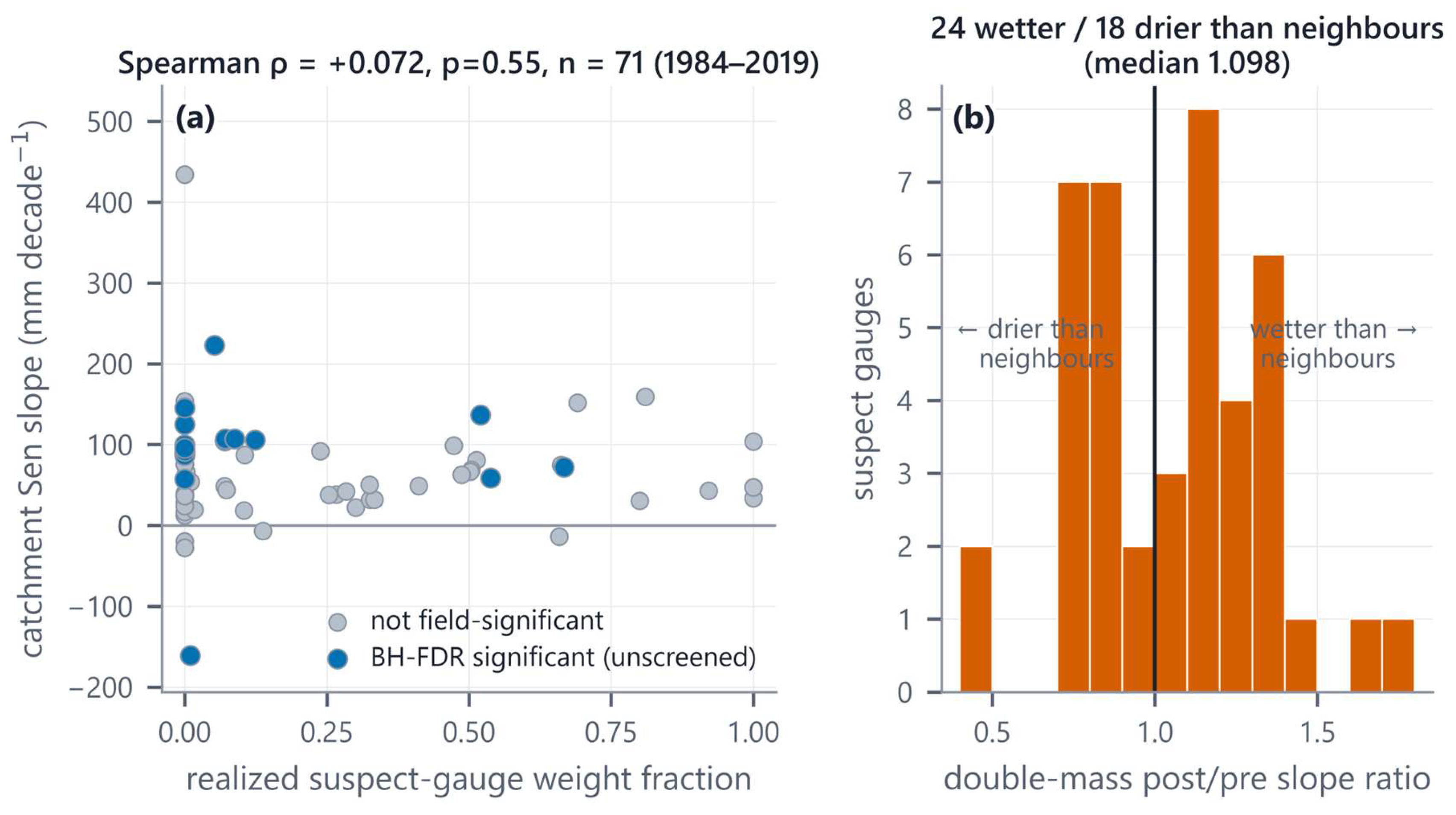
Figure 5. What catchment-level screening can show. (a) Raw-significant increase rate against retained family size for all 18 scenario × threshold combinations, with the unscreened reference (star, dashed rule) at 30/71 = 0.423. The rate does not fall materially under the primary scenario; across the family it moves in both directions (7 combinations above the reference, 11 below), the low outliers being scenario C, which removes 49 of 71 catchments. (b) Fate of the 16 unscreened field-significant increases (rows, ordered by Sen slope) across the 18 combinations (columns, grouped by scenario). Blue = survives false-discovery-rate control in the screened family; pale grey = removed from the family by the screen. A third conceivable outcome — retained by the screen but losing significance — never occurs (0 of 288 catchment-outcomes) and therefore has no cell in the matrix; that count is close to structurally guaranteed, because a retained catchment keeps its original series unchanged and the three most suspect-heavy of the 16 are removed in all 18 combinations (Section 3.5). The test that can change a verdict is the leave-suspect-out reconstruction of Section 3.6 and Table 8 and Table 9, which costs two of the 16 their field significance and creates three new detections.

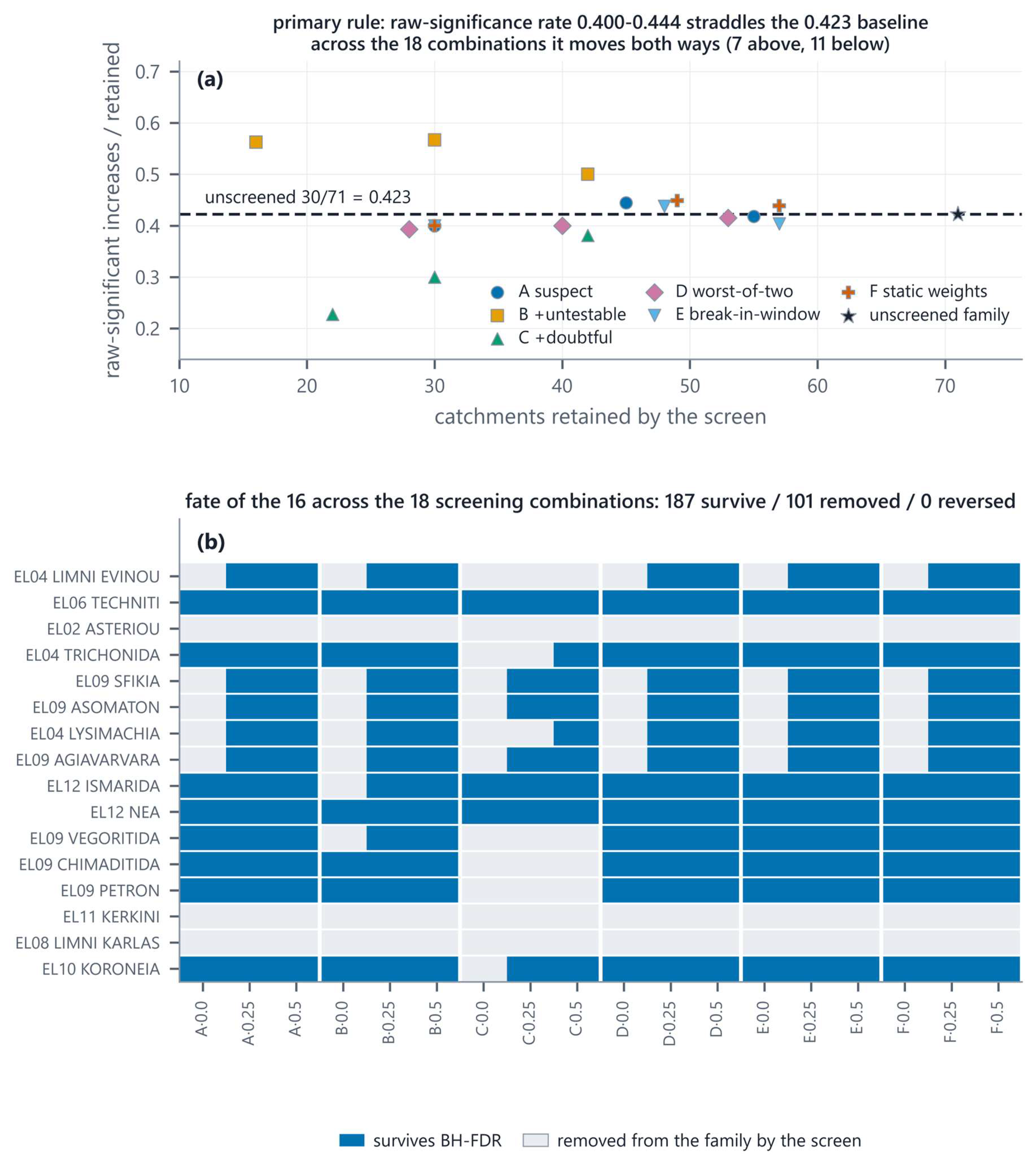
Table 7. Diagnostics separating “screening removed the signal” from “screening removed catchments”.

Diagnostic	Value	Reading
Raw-significant increase rate, unscreened	30/71 = 0.423	reference rate
Raw rate, scenario A at thresholds 0 / 0.25 / 0.5	0.400 / 0.444 / 0.418	does not fall materially under the primary rule; would fall if inhomogeneity manufactured the increases
Raw rate, full range over the 18 combinations	0.227–0.567 (7 above the reference, 11 below)	moves in both directions; the “does not fall” reading is scoped to the primary scenario, not to the family
Spearman ρ (realized suspect weight, Sen slope)	+0.072 (p = 0.548, n = 71)	no dose–response; static-weight version +0.024 (p = 0.840)
Median Sen by suspect-weight stratum	0: +48.3 (n = 30); 0–0.25: +65.6 (n = 15); > 0.25: +49.5 (n = 26)	flat, and not ordered with suspect weight
Direction of shift at suspect gauges (double-mass post/pre slope)	24 wetter / 18 drier (n = 42, median 1.098, range 0.406–1.705)	a network-wide artefact would be one-signed
SNHT-located relative breaks at suspect gauges inside 1995–2004 inclusive (on the wider 1995–2005 window, the one the deposited diagnostic table uses: 18 of 42, Pettitt-located 24 of 42)	17 of 42 (Pettitt-located: 23 of 42)	a genuine relative break cluster, not merely an absolute one
Catchments retained by the drop-only screen that then lost BH-FDR significance, summed over all 18 combinations	0 of 288 catchment-outcomes (187 survive, 101 removed)	the increases are not confined to the suspect-supported network — but a retained series is unchanged by construction, so this is not a test of the data (Section 3.5)
Of the 16, reversals under the primary leave-suspect-out reconstruction (L1)	14 survive, 2 lose field significance, 3 new detections appear on 2 distinct series (16 − 2 + 3 = 17)	the decisive count: verdicts measured on rebuilt series (Section 3.6)
Raw rate and median slope under L1, matched catchments	rate 0.439 → 0.485; median +55.6 → +63.9 mm decade⁻¹	both rise; the artefact hypothesis predicts both fall

Table 8. The leave-suspect-out reconstruction. Each rule deletes a class of gauges from every catchment’s weight vector, renormalizes the surviving weights under the areal product’s own per-year policy, rebuilds the areal annual series and re-estimates the trend. “Matched BH ↑” applies Benjamini–Hochberg to the drop-nothing reconstruction restricted to the same catchments, so the comparison is paired. L0 is the fail-closed parity row: it must reproduce the published family exactly. The BH columns count hypotheses rather than distinct series, so the nominal counts include reconstructed catchments that collapse to a single identical series; the deduplicated counts for the primary and most-affected rules are given in Section 3.6.

Rule	Gauges deleted	n	Lost: no gauge / too short	raw ↑/↓	BH ↑/↓	median (mm dec⁻¹)	Matched BH ↑/↓	Matched median	Of the 16: kept / lost	Gained
L0 — delete nothing (parity)	0	71	0 / 0	30/1	16/1	+54.2	16/1	+54.2	16 / 0	0
L1 — suspect (primary)	42	66	3 / 2	32/1	17/1	+63.9	16/1	+55.6	14 / 2	3
L2 — suspect + untestable	61	55	15 / 1	31/1	20/1	+75.7	16/1	+66.5	14 / 2	6
L3 — suspect + doubtful	72	62	6 / 3	26/1	13/1	+65.8	16/1	+52.2	10 / 6	3
L4 — worst of ratio/difference	49	65	4 / 2	29/1	17/1	+57.0	16/1	+54.2	14 / 2	3
L5 — suspect with in-window break	38	67	2 / 2	33/1	17/1	+65.2	16/1	+54.2	14 / 2	3
L6 — suspect, BH-FDR within test	21	70	0 / 1	31/1	16/1	+62.8	16/1	+55.6	14 / 2	2
L7 — suspect, BH-FDR over all 672 tests	20	70	0 / 1	31/1	16/1	+62.8	16/1	+55.6	14 / 2	2

Table 9. The 16 field-significant increases under the primary leave-suspect-out rule (L1), together with the single field-significant decrease (EL13_APOSELEMI) shown in italics, ordered by outcome then by the static weight deleted. “w deleted” is the fraction of the catchment’s static Thiessen weight carried by its suspect gauges. “Sen before” and “p before” are the drop-nothing reconstruction values of Section 3.6 rather than the published ones, so every comparison in this table is reconstruction against reconstruction. Every one of the 16 remains reconstructible; none changes sign. p is the ungated lag-1 Hamed–Rao p-value; the Benjamini–Hochberg verdict is taken against the matched baseline. The “lost” outcome is the reversal counted in Section 3.6: the catchment no longer holds field significance against that baseline, and both catchments it applies to keep a positive, still raw-significant slope. “Shift” is the difference of the unrounded Sen slopes, rounded once, so in three rows it differs by 0.1 from the difference of the two rounded columns printed beside it.

Catchment	Gauges	w deleted	Years before → after	Sen before	Sen after	Shift	p before	p after	Outcome
EL02_ASTERIOU	3 → 2	0.620	35 → 35	+136.5	+90.7	−45.8	0.0051	0.0309	lost (still raw-significant)
EL08_LIMNI_KARLAS	4 → 3	0.566	35 → 35	+58.8	+50.5	−8.4	0.0070	0.0409	lost (still raw-significant)
EL11_KERKINI	7 → 4	0.756	36 → 36	+72.1	+71.8	−0.3	0.0079	0.0006	retained
EL04_LYSIMACHIA	10 → 9	0.115	35 → 35	+105.5	+117.1	+11.6	0.0015	0.0026	retained
EL13_APOSELEMI (the decrease)	5 → 4	0.026	35 → 35	−161.0	−163.6	−2.6	0.0005	0.0005	retained
EL04_LIMNI_EVINOU	6 → 5	0.020	33 → 33	+223.0	+225.8	+2.9	0.0001	0.0002	retained
EL09_SFIKIA	3 → 2	0.006	30 → 28	+107.2	+105.2	−2.1	0.0074	0.0037	retained
EL09_ASOMATON	3 → 2	0.004	30 → 28	+107.2	+102.9	−4.3	0.0060	0.0037	retained
EL09_AGIAVARVARA	3 → 2	0.004	30 → 28	+105.0	+101.6	−3.4	0.0074	0.0037	retained
EL06_TECHNITI	2 → 2	0.000	31 → 31	+145.5	+145.5	0.0	0.0016	0.0016	retained (unchanged)
EL04_TRICHONIDA	5 → 5	0.000	35 → 35	+125.0	+125.0	0.0	0.0021	0.0021	retained (unchanged)
EL09_VEGORITIDA	6 → 6	0.000	36 → 36	+91.7	+91.7	0.0	0.0012	0.0012	retained (unchanged)
EL09_PETRON	3 → 3	0.000	32 → 32	+86.8	+86.8	0.0	0.0014	0.0014	retained (unchanged)
EL10_KORONEIA	5 → 5	0.000	36 → 36	+57.0	+57.0	0.0	0.0054	0.0054	retained (unchanged)
EL09_CHIMADITIDA	2 → 2	0.000	32 → 32	+89.5	+89.5	0.0	0.0020	0.0020	retained (unchanged)
EL12_ISMARIDA	5 → 5	0.000	35 → 35	+99.8	+99.8	0.0	0.0029	0.0029	retained (unchanged)
EL12_NEA	1 → 1	0.000	34 → 34	+95.5	+95.5	0.0	0.0049	0.0049	retained (unchanged)

The rate. Unscreened, 30 of 71 catchments are raw-significant increases, a rate of 0.423. Under the primary scenario A the rate is 0.400 (12/30) at threshold 0, 0.444 (20/45) at 0.25 and 0.418 (23/55) at 0.5 — numerically indistinguishable from the unscreened 0.423, and not falling materially (Figure 5a). No significance test is attached to that comparison; the informative statement is the direction of the change and its spread. That statement holds for the primary scenario and must not be generalized to the family. Across all 18 combinations the rate ranges from 0.227 to 0.567 and moves in both directions: above the unscreened rate in 7 combinations and below it in 11. The lowest come from scenario C, which drops any catchment carrying any doubtful or suspect weight and so removes 49 of 71, leaving a small and spatially unrepresentative residue; the highest from scenario B, which also removes the untestable-weight catchments and retains as few as 16. The defensible summary is that the rate does not fall materially under the primary rule and is not systematically directional across the family — not that it fails to fall in every combination, which is untrue.

Dose–response. The Spearman rank correlation between realized suspect weight fraction and catchment Sen slope is +0.072 (p = 0.548, n = 71) — no association at all (Figure 4a). The static-weight version is +0.024 (p = 0.840). Stratified: catchments with zero suspect weight have a median slope of +48.3 mm decade⁻¹ (n = 30), those with 0 < suspect weight ≤ 0.25 have +65.6 (n = 15), and those above 0.25 have +49.5 (n = 26). The gradient is flat and not ordered with suspect weight.

Sign symmetry. Among the 42 suspect gauges, the double-mass post/pre slope ratio is above 1 for 24 and below 1 for 18, with a median of 1.098 and a full range of 0.406 to 1.705 (Figure 4b). Relative breaks in this network are bidirectional — some gauges started reading high relative to their neighbours, others low. A network-wide artefact capable of manufacturing a coherent wetting field would have to be overwhelmingly one-signed; this is not. That balance is network-wide, taken over all 42 flagged gauges rather than over the flagged gauges that carry weight in the 16 field-significant increases; the direction restricted to those 16 is reported in Section 3.6, where deleting their flagged gauges leaves a median slope shift of exactly zero (8 unchanged, 6 falling, 2 rising).

Retention count, and what it is worth. Across the 18 scenario × threshold combinations, the 16 field-significant increases generate 288 catchment-outcomes: 187 survive and 101 are removed from the family by the screen. The number retained by the screen and then losing false-discovery-rate significance is zero (Figure 5b).

That count is real, and it is also close to structurally guaranteed, so what it does and does not show is worth stating plainly. A retained catchment’s areal series, Theil–Sen slope and Hamed–Rao p are bit-identical to the unscreened ones, and at threshold 0.00 the retained set carries no suspect weight by construction, so the catchments most exposed to inhomogeneity are excluded from the tally rather than tested by it. The three members of the 16 that carry more than half their realized weight on suspect gauges — EL11_KERKINI (0.667), EL08_LIMNI_KARLAS (0.538) and EL02_ASTERIOU (0.520) — are screened out in all 18 combinations, and so are structurally incapable of contributing a reversal. They account for 54 of the 101 removals. The zero is therefore evidence that the increases are not confined to the suspect-supported part of the network — a real and useful statement — and it is not evidence that removing the suspect data leaves the trends unchanged. That second question requires rebuilding the series, and Section 3.6 does so — on all three of these catchments, which is precisely where it changes the answer.

3.6. The Decisive Test: Leave-Suspect-Out Reconstruction

Deleting the suspect gauges, renormalizing the Thiessen weights over the survivors and rebuilding every areal series (Section 2.2.7) converts the screen from a subset statement into a test. The drop-nothing reconstruction reproduces the published family exactly — n = 71, 30 raw increases and 1 raw decrease, 16 and 1 surviving false-discovery-rate control, the same 16 catchments and the same decrease — with per-catchment slopes agreeing to within 0.091 mm decade⁻¹ (the largest single deviation, at EL13_FANEROMENIS) and the network median to within 0.063 mm decade⁻¹ of the published values, the residual being the sub-millimetre effect of storing weights to four decimals. All comparisons below are reconstruction against reconstruction, so that residual cancels.

The primary rule (L1) costs two of the 16 their field significance and creates three new detections. Deleting all 42 suspect gauges leaves 66 of the 71 catchments reconstructible. Three lose every gauge they had (EL05_PIGESAOOU, EL09_PRAMORITSA, EL13_KOURNA) and two fall below the minimum-length rule (EL10_PIKROLIMNI, EL12_IASIO); none of the five was field-significant, and their drop-nothing reconstruction slopes were +33.7, +103.8, +47.1, +47.1 and +159.1 mm decade⁻¹ at p = 0.40, 0.11, 0.73, 0.60 and 0.040. Every one of the 16 keeps a reconstructible series. Against the matched baseline, 14 of the 16 retain false-discovery-rate significance and 2 lose it — EL02_ASTERIOU and EL08_LIMNI_KARLAS — while 3 catchments that were not field-significant become so: EL04_AMVRAKIA, EL04_OZEROS and EL08_LIMNI_SMOKOVOU. The arithmetic is therefore 16 − 2 + 3 = 17, and the reconstruction is not a purely subtractive operation: it creates detections as well as removing them.

The three new detections rest on only two distinct series. Under this rule EL04_AMVRAKIA and EL04_OZEROS both lose every gauge but ΛEΠEΝOΥ and reconstruct to the identical 30-year record (+144.8 mm decade⁻¹, p = 0.0072 in both), so a single reconstructed series enters the Benjamini–Hochberg family as two hypotheses; EL08_LIMNI_SMOKOVOU is independent of them, losing 0.537 of its static weight and rising from +62.9 to +83.7 mm decade⁻¹ with p from 0.0489 to 0.0111. Catchments resting on the same single record — or, more generally, on gauge sets whose renormalized weights coincide — carry identical series and so enter the Benjamini–Hochberg family as duplicate hypotheses; sharing a gauge list is not by itself sufficient, because unequal Thiessen areas renormalize to different weights, so duplicates are identified on the values of the reconstructed series rather than on their gauge lists. This is a property of the published family as well as of the reconstructed ones — that family carries four duplicate groups of its own, collapsing its 71 catchments onto 63 distinct series without changing its 16 increases and 1 decrease — and it inflates the hypothesis count without adding information.

The field count is 17 increases and 1 decrease, against 16 and 1 on the matched baseline (Table 8). Collapsing each family to distinct reconstructed series before the correction — one hypothesis per identical series, represented by a single member of each group, identical series carrying identical p so that the choice is a label rather than a selection — makes that inflation measurable rather than rhetorical: the reconstructed family of 66 holds five duplicate groups and collapses to 57 distinct series, the matched baseline four groups and 58, and the Benjamini–Hochberg step-up on the collapsed families returns 16 increases and 1 decrease on both, with no catchment changing verdict in either direction. On distinct series the screened arithmetic is therefore 16 − 2 + 2 = 16 — the 14 survivors plus the two distinct new series — and the nominal gain of one increase over the baseline is entirely the duplicate hypothesis that the shared ΛEΠEΝOΥ record contributes twice.

The reversals fall exactly where the drop-only screen was blind. Both of the two are drawn from the three members of the 16 that carry more than half their realized weight on suspect gauges (Section 3.5) — the three that catchment-level screening removed from its own tally in all 18 combinations. The third, EL11_KERKINI, loses 76% of its static weight and gains evidence: its slope barely moves (+72.1 to +71.8 mm decade⁻¹) while its p falls from 0.0079 to 0.00063. That gain is support concentration and should be read as such rather than as independent confirmation: the reconstruction leaves the catchment resting on four surviving gauges instead of seven, with the dominant share passing to AΧΛAΔOΧΩΡΙ — which is also the single gauge the AR(1) recalibration promotes into the suspect class (Section 3.2), so Kerkini is flagged at the other end of the calibration range rather than cleared by it. This is the clearest possible demonstration that the two procedures are not measuring the same thing: the drop-only count was zero precisely because it excluded the catchments where the reconstruction finds all of its action.

The two reversals deserve their detail rather than a count, because they are not equivalent (Table 9). Both keep a positive slope; neither changes sign. EL02_ASTERIOU loses 62% of its static weight, keeps all 35 years, and falls from +136.5 to +90.7 mm decade⁻¹ with p moving from 0.0051 to 0.0309 — still raw-significant at 5%, demoted only by the multiplicity threshold. EL08_LIMNI_KARLAS loses 57% of its weight, keeps all 35 years, and falls from +58.8 to +50.5 with p from 0.0070 to 0.0409 — again still raw-significant. Neither is a collapse of support: the clearest instance of that is EL10_DOIRANI, a two-gauge catchment reduced to one whose record halves from 33 years to 18 and whose slope falls from +74.7 to +38.3 mm decade⁻¹ at p 0.018 to 0.395. Doirani is not among the 16 — it is nominally but not field-significant on the baseline — but it is the clearest single demonstration that a catchment resting on two gauges cannot survive losing one, and it is why any such change is reported here as a support loss rather than as evidence of inhomogeneity.

The aggregate moves the other way — under this calibration. On the same 66 catchments the raw-significant increase rate rises from 0.439 on the matched baseline to 0.485 after reconstruction, and the median slope from +55.6 to +63.9 mm decade⁻¹. Deleting the suspect gauges makes more catchments significant, not fewer. This direction is specific to the i.i.d. calibration of the battery: on the smaller suspect set an AR(1)-calibrated battery flags, both quantities move the other way (Section 3.2, Table 5), so the aggregate direction is not a robust finding and only the field-significance verdict is. Of the 66 reconstructed catchments, 30 carry no suspect gauge and are numerically unchanged; among the 36 that do lose weight the median slope shift is −0.4 mm decade⁻¹ and 24 shift by more than 10 mm decade⁻¹ in absolute value, in both directions (full range −118.5 to +114.4). Among the 16 the median shift is exactly zero: 8 are unchanged, 6 fall and 2 rise.

The scenario range (L2–L7). The two reversals are the same two under every variant except the deliberately over-conservative one. Deleting untestable gauges as well (L2) leaves 55 catchments — 15 lose all support, essentially the insular set — and gives the same two reversals among the 16, with six newly field-significant catchments (again including the ΛEΠEΝOΥ pair, so five distinct series); that reconciles the L2 row of Table 8 (16 − 2 + 6 = 20). The worst-of-ratio-and-difference rule (L4) gives the same two, as does restricting to suspect gauges with an in-window break (L5). Both multiplicity-controlled rules (L6, L7) delete only 21 and 20 gauges, lose no catchment to total gauge loss, and give the same two reversals, with the ΛEΠEΝOΥ pair as the only gain. Only L3 — deleting suspect and doubtful gauges, 72 of 187 — moves the field materially: 6 of the 16 reverse, the field falls to 13 increases, and the raw rate falls to 0.419 against a matched baseline of 0.435. That is the one variant in which the aggregate evidence weakens, and it is also the variant that removes 39% of the weight-carrying network, including every gauge that merely returned two rejections out of four. It is reported rather than omitted, and it is not treated as the primary answer.

Verdict. The honest summary is two-sided. Individual catchment verdicts in this field are fragile: two of the 16, and up to six under the most aggressive rule, do not survive having their flagged gauges deleted, so any use of a single catchment’s field-significant increase as a local climatic claim is unsafe. The field-level conclusion is not fragile, and it moves against the artefact hypothesis rather than with it: 14 of the 16 keep their field significance under every gauge-removal rule but L3 — which leaves 10 — and 14 or 15 of the 16 under every null calibration tested — 15 under the serial and calendar recalibrations, 14 under the distributional one (Table 6) — three new detections appear on two distinct reconstructed series, and no reversal involves a change of sign. What would have supported the artefact hypothesis — a falling rate, a falling median, reversals concentrated in the suspect-heavy catchments — is not what the reconstruction produces, except in L3, where it produces a falling rate at the cost of deleting most of the network.

The dose–response, and which end of the range is the harder test. Ordering every rule by the number of gauges it deletes turns that invariance into a dose–response rather than an assertion, and the ordering is informative in a way the individual rows are not. Against a like-for-like denominator — all 16 field-significant increases are reconstructible under every one of the nine rules, so no comparison below is confounded by a shrinking family — the number of the 16 whose weight vector the rule actually touches rises monotonically with dose: 0 gauges deleted touches none, 4 touches two, 20 touches seven, 21, 38, 42 and 49 each touch eight, 61 touches ten and 72 touches thirteen. The number keeping field significance falls far more slowly: 16, 15, then 14 across the whole span from 20 to 61 deleted gauges, and 10 only at 72. The consequence runs opposite to the way the calibration question is usually posed. The AR(1)-recalibrated set, which deletes 4 gauges, perturbs only two of the 16 and is therefore the weakest perturbation in the family; the i.i.d.-calibrated primary rule, which deletes 42, perturbs eight and leaves 14 standing. Whatever is true about the relative sizing of the two nulls — and Section 3.2 measures it rather than assuming it — the primary calibration subjects the field result to four times as much disturbance as the recalibrated one and the result survives, so the choice of primary is conservative in the direction that matters for the conclusion drawn from it. The two reversals separate cleanly along the same axis: EL02_ASTERIOU reverses at every non-zero dose including the 4-gauge one, which makes it a property of that catchment’s own support rather than of any screening threshold, while EL08_LIMNI_KARLAS enters at 20 and is stable from there. The remaining four reversals appear only at 72, the rule that additionally deletes every doubtful gauge, which locates the breakpoint of the whole family at the doubtful class rather than anywhere in the suspect one.

3.7. The Artefact the Homogeneity Screen Cannot See

The screen’s second layer earns its place on a catchment where the first layer returns nothing. The Cretan Aposelemi catchment (EL13) is the only field-significant decrease in the trend family (−161.0 mm decade⁻¹, p = 0.00052, n = 35 years). Its realized weight is 79.2% useful, 19.8% untestable and just 0.9% suspect — the relative-homogeneity battery flags essentially nothing, and the catchment survives homogeneity screening at every threshold above zero.

Yet the dominant part of the decrease is, under the decomposition tested here, attributable to network composition (Figure 6). The catchment’s five weighted gauges divide the area very unequally: static weights of 0.587 (AΓ. ΓEΩΡΓΙOΣ), 0.344 (ABΔOΥ), 0.026 (AΡMAΧA), 0.021 (ΚAΣΤEΛΙ) and 0.021 (ΚAΛAMAΥΚA). The two dominant gauges are also the wettest — mean annual totals of 989 mm and 793 mm over the years they report — and both terminate early, in 2000 and 1994 respectively. The three residual gauges are drier: 753 mm (AΡMAΧA), 576 mm (ΚAΣΤEΛΙ) and 641 mm (ΚAΛAMAΥΚA), and AΡMAΧA itself ends in 1994 alongside ABΔOΥ, so beyond 2000 only ΚAΣΤEΛΙ (to 2011) and ΚAΛAMAΥΚA (to 2018) still report. Because the areal estimate renormalizes each year over whoever reported, those two inherit the vacated share. Averaged over the 35 catchment-years, ΚAΛAMAΥΚA’s realized weight is 0.367 — 17.3 times its static weight of 0.0212, which the list above rounds to 0.021 — and from 2012 onwards it alone constitutes the catchment’s “areal” precipitation.

The consequence is a step in the areal series with no step in any gauge series: the catchment mean falls from 898 mm over 1984–2000 to 576 mm over 2001–2018, a drop of 322 mm, while ΚAΛAMAΥΚA’s own record over the same window trends at only −45.4 mm decade⁻¹ (p = 0.096, n = 30), not significant and less than a third of the areal slope. The areal series is therefore not measuring a drying catchment of the magnitude it reports; the dominant part of the slope is a migration down the catchment’s own precipitation gradient, executed by the archive. Section 4.4 measures what survives removal of that level offset — 27% to 54% of the slope, a residual that brackets ΚAΛAMAΥΚA’s own non-significant −45.4 mm decade⁻¹ — so a smaller genuine decrease is not excluded, and this design cannot separate one from the post-2012 collapse onto a single gauge.

Aposelemi is the clearest case but not a unique one. In 8 of the 73 catchments the dominant gauge’s realized weight exceeds twice its static weight — 7 of the 71 that enter the trend family, the eighth (EL12_GRATINI) being one of the two catchments too short to be tested. The list includes EL06_TECHNITI, one of the 16 field-significant increases, where a gauge with a static weight of 0.042 does 0.660 of the work — an amplification of 15.7. Weight amplification is a property of the network’s mortality schedule, and it operates on increases and decreases alike; it is not a mechanism that conveniently only afflicts the results one is disinclined to believe.

The symmetry, performed. That last sentence is a claim about the method, so the same dissection was run on EL06_TECHNITI that Figure 6 runs on Aposelemi, with Aposelemi retained as a positive control that must reproduce its published numbers before the new catchment is reported. The mechanism is the same one, in mirror image, and even on the same schedule. Techniti’s two weighted gauges are ΧAΛAΝΔΡΙ, holding 0.958 of the static weight, and AΛMΥΡOΠOΤAMOΣ, holding 0.042. ΧAΛAΝΔΡΙ’s record ends in 2000 — the same year AΓ. ΓEΩΡΓΙOΣ leaves Aposelemi — after which the catchment rests on AΛMΥΡOΠOΤAMOΣ alone, whose realized weight over the 31 catchment-years is 0.660, or 15.7 times its static share. The displacement runs up the precipitation gradient rather than down it: AΛMΥΡOΠOΤAMOΣ averages 730 mm against ΧAΛAΝΔΡΙ’s 413 mm, and the catchment mean steps from 480 mm over 1984–2000 to 833 mm over 2001–2014, a rise of 353 mm, against Aposelemi’s fall of 322 mm. Both gauges are classified useful, so no removal rule touches the catchment and its series is unchanged at 31 years under every scenario in Table 9.

One quantity separates the two cases, and it is the one that matters. ΚAΛAMAΥΚA’s own record trends at −45.4 mm decade⁻¹ at p = 0.096, not significant and less than a third of Aposelemi’s areal slope, so the areal decrease is largely composition. AΛMΥΡOΠOΤAMOΣ’s own record trends at +100.6 mm decade⁻¹ at p = 0.030 over the same 31 years — significant in its own right, and 69% of the +145.5 the areal series reports. Composition inflates Techniti’s increase by roughly half again; it does not manufacture it. The symmetry the paragraph above claims is therefore real as a mechanism and asymmetric in this instance as a verdict, and it is reported that way: the same archival process that fabricates most of one field-significant decrease exaggerates, but does not invent, one field-significant increase.

The diagnostic, applied to the screen’s own products. Leave-suspect-out deletion is itself an amplification operation — it renormalizes the weight of whatever survives — so the test of Section 3.7 has to be turned on the reconstructions of Section 3.6 as well as on the published product, or the screen exempts itself from its own test. Table 10 does that for all nine rules — the eight deletion rules of Section 3.6 and, as L8, the 4-gauge recalibrated deletion that is the low end of the dose–response. The answer depends entirely on the reference point, and that dependence is the finding. Measured the way the published diagnostic measures it, renormalizing the static share over the surviving gauges, the reconstructions look better than the product: the count falls from 7 of 71 to 5 of 66 under the primary rule and the median amplification is exactly 1.000 under every rule. But that measure is structurally blind to the deletion, because a catchment reduced to one surviving gauge has realized weight equal to static weight and scores exactly 1.0 whatever the original network looked like.

Measured against the original network the primary rule more than doubles the count, 7 → 16, and lifts the of-the-16 field-significant increases sitting on an amplified gauge from 4 to 7. Naming those seven answers the question the count provokes, and the answer is not a random draw from the 16. Four of them — EL04_LIMNI_EVINOU, EL06_TECHNITI, EL09_PETRON and EL12_ISMARIDA — are amplified in the published product before anything is deleted, and all four survive the primary rule unchanged. The three the deletion adds are EL02_ASTERIOU, EL08_LIMNI_KARLAS and EL11_KERKINI, which are exactly the three members of the 16 that carry more than half their realized weight on suspect gauges (Section 3.6): the two reversals and the one catchment whose evidence strengthens. Concentration onto a gauge the published product barely used therefore falls precisely on the three catchments the reconstruction acts hardest on, which is both why they move and a reason to read the direction in which they move as a property of the deletion rather than of the climate.

The three new detections are outside this list by construction, since it is drawn from the 16 baseline increases; their own concentration factors are given above. This bears directly on the three new detections of Section 3.6: EL04_AMVRAKIA is itself an amplification product, ΛEΠEΝOΥ carrying all of the catchment on 0.171 of the original static weight (5.8×), and EL04_OZEROS reconstructs to the same ΛEΠEΝOΥ series, so the two are one piece of evidence rather than two; only EL08_LIMNI_SMOKOVOU, at 2.0×, retains four gauges. The new discoveries are accordingly reported as what the reconstruction produces, not as independent confirmations, and the same caution applies to EL11_KERKINI, whose gain in evidence under L1 (Section 3.6) is a 4.0× concentration onto AΧΛAΔOΧΩΡΙ. Throughout, deletion-amplified single-gauge dependence is a property of the aggregation topology — the realized weights of whichever gauges survive must sum to one — and not evidence that the surviving gauges are homogeneous.

4. Discussion

4.1. What the Screen Establishes, and What It Does Not

The results of Section 3.5 and Section 3.6 answer two different questions and must be kept apart, because the weaker one is the more quotable.

What catchment-level screening establishes. The 18 combinations establish that the field’s increases are not confined to the suspect-supported part of the network: a family assembled from catchments carrying no suspect weight at all still returns a comparable raw-significance rate and a comparable median slope. What they cannot establish is that removing the suspect data leaves the trends unchanged, because they never remove the data. Reporting a zero reversal count from such a procedure as the central result would be, at the strictest threshold, reporting a definition. An earlier version of this analysis did exactly that, and the correction is worth stating explicitly rather than quietly: a screen that only partitions a family tests membership, not measurement.

What the reconstruction establishes. Deleting the flagged gauges and rebuilding does change answers, and the changes are informative in both directions (Section 3.6). The artefact hypothesis makes a directional prediction — remove the questionable gauges and the wetting should weaken — and the reconstruction fails to reproduce that prediction at field level under every gauge-removal rule but the most aggressive, L3, which deletes 72 of the 187 weight-carrying gauges, costs 6 of the 16 their field significance and leaves 10. Detectable, non-shared gauge discontinuities alone therefore do not explain the field-level result under the rules tested; the prediction does hold for a minority of individual catchments under every rule, individual catchment verdicts are correspondingly fragile, and the aggregate rate and median are evidence in neither direction (Section 3.2 and Section 4.5).

The distinction that matters for a reader of the parent trend field is therefore between the count and the map. The count is robust except under the most aggressive rule: 14 or 15 of the 16 under every gauge-removal rule and every null calibration tested but L3, which deletes 39% of the weight-carrying network and leaves 10. The identity of the catchments is not, and the two that change status under the primary rule are two of the three a drop-only screen was structurally unable to examine.

None of this is validation. A screen cannot validate; it can only fail to falsify. The trends could still be wrong for reasons neither layer can address — a bias shared by candidate and reference (Section 4.2), a change in the instrument population common to the whole network, a gradual drift, an error in the interpolation, or simple sampling variability in a 36-year window. What the exercise removes from the table is one specific alternative explanation, and only that one: that the field’s increases were manufactured, at field level, by the discontinuities in the gauge records that carry them.

4.2. Two Bounding Caveats, of Opposite Sign

The most important limitation is structural and cannot be engineered away within this design. The reference neighbours are themselves untested gauges from the same archive. A relative test detects a change in the candidate relative to its reference; a break shared by candidate and reference cancels in the ratio and is invisible. Since neighbouring stations in a national network are frequently operated by the same authority, re-equipped in the same programme, relocated under the same policy and digitized in the same campaign, shared breaks are not a hypothetical concern. The converse ambiguity is equally structural and equally unresolved here: a ratio series steps if the composite steps, so a detected relative break cannot be attributed to the candidate rather than to its reference — and the composite is itself rebuilt each year from whichever admitted neighbours reported, which is the third source of ratio persistence quantified in Section 3.2. Two things bound it.

The composite does not inherit the level step, because every neighbour is rescaled to the candidate’s mean over their common years before it is averaged, so a neighbour entering or leaving cannot move the reference by the amount its own mean differs from the candidate’s. And a fixed-support reference, restricted to years in which every admitted neighbour reports, is not an available alternative on this archive: that restriction leaves most tested gauges below the twenty-year floor the battery requires, so it would trade the bias for a much smaller and differently selected tested set. The rescaling is also done pair by pair, over each neighbour’s own overlap with the candidate, so a neighbour whose overlap sits mostly on one side of a candidate break carries that side’s candidate level into the composite, and a break coinciding with a change of neighbour membership is therefore partly absorbed by the reference rather than isolated by it.

The screen is also a single pass: neighbours are admitted on the criteria of Section 2.2.2, none of which is a homogeneity verdict, so a composite may contain gauges that the same pass later classes suspect, and the battery is not re-run with those excluded. And because a reference value exists for a year when at least two admitted neighbours report it, the number of neighbours behind the composite varies from year to year within a series, so the reference is not equally well determined in every year, and that per-year count is not carried into the test statistics. This is why no per-gauge label here is used as a claim about an individual station’s history, and why the k = 3 neighbour-set sensitivity is carried as a screening scenario rather than as a robustness certificate.

The detection of inhomogeneity here is therefore bounded below and not above: what a relative battery can see is a subset of what is there, so this bias pushes the true number of inhomogeneous gauges above the detected set. It does not follow that the flagged set is a bound on that number, because a second bias runs the other way — the i.i.d. critical values applied to the persistent test series of Section 3.2 inflate the flagged set relative to the genuinely broken one. The 42 suspect gauges are therefore neither a count nor a one-sided bound: two biases of opposite sign act on them. Section 3.2 quantifies the second and puts a calibration-dependent range on the detectably inhomogeneous count, 4 gauges against 42, and nothing in the field-level verdict depends on choosing between them: 14 of the 16 field-significant increases survive deletion of the 42 and 15 of the 16 survive deletion of the 4.

Two consequences follow. The class labels should be read as “detectably inhomogeneous relative to neighbours”, not as “inhomogeneous”, and useful is the weakest of the three, meaning only that a relative test found nothing. And, most consequential for the negative result, the field-level invariance in Section 3.5 and Section 3.6 is invariance to detectable, non-shared inhomogeneity: a synchronized network-wide change would pass through the entire screen undetected. Only an independent, differently-constructed dataset — a homogenized gridded product, a reanalysis, a different observing system — can address that, and such comparisons are a different exercise from the one performed here. For Greece the candidates now exist: a homogenized 1 km daily gridded precipitation and temperature product [38], gridded and reanalysis intercomparisons [39], and independent national trend assessments [40,41]. Their value as a cross-check is real but bounded: a product that is homogenized but draws on the same gauges provides a processing-robustness check rather than a data-independent one. One such bounded comparison is performed here, where it bears directly on the second layer’s worked example — Section 4.4 reads the Aposelemi composite against CLIMADAT-GRid primarily at the level, keeping its slope only as a consistency estimate.

The same logic applies to the tests themselves. All four are single-break detectors. Multiple breaks, gradual drift — vegetation growth around a gauge is the classic example, and it produces exactly the slow relative decline that a step test is least able to see — and slowly-changing exposure are outside their reach. Nor is the screen validated end to end against a known truth. The reconstruction and trend-family paths are proved against the published product itself (Section 2.2.1 and Section 2.3.2, and the L0 parity row of Table 8) and the four implementations against idealised series (Section 2.2.5), but the classification layer’s false-classification rate, its power and its break-year accuracy have not been established on synthetic networks carrying spatial climate covariance, precipitation skew, missingness and gauge entry and exit. Until such a benchmark exists, the counts reported here are counts under this battery rather than calibrated detection rates, and building one — with reference-admission failures and catchment reconstruction error reported on it — is the natural next step for this screen.

4.3. The 19 Untestable Gauges Are a Finding, Not Only a Limitation

Nineteen of 187 weight-carrying gauges could not be tested at all, and 11 catchments rest entirely on such gauges — the nine Aegean-island lakes and the two Prespa lakes on the northern border — so for those 11 the conclusion of this screen is no information: not support, and not doubt (Section 3.3). The companion catchment-scale hydroclimatic analysis by the present authors reaches the same boundary from the other side, treating island and single-gauge catchments as indicative throughout. It would be convenient to treat these as a small residual. They are not, for two reasons.

They are systematically selected. A gauge is untestable precisely when it has too few correlated neighbours — that is, when it is isolated or insular. But isolation is also what gives a gauge a large Thiessen weight: in a sparse region one gauge represents a large area. The untestability of a gauge and its influence on the areal field are therefore positively correlated by construction, which is the opposite of the benign case. Relative homogeneity testing is systematically blind in exactly the places where a single gauge’s behaviour matters most.

They are also a structural finding about sparse networks. Here the untestable set is essentially the Aegean islands plus the isolated northern border sites, and any relative method applied to an insular or mountainous network will encounter the same thing. The honest response is to report it as its own class, quantify the weight it carries, and extend the reported range with a scenario that treats untestable weight as suspect — scenario B, which drops as many as 55 of 71 catchments, and its reconstruction counterpart L2, under which 15 catchments lose every gauge they had and simply cease to have an areal series. Neither rescues the untestable set; both quantify what is at stake in it. Reporting untestable gauges as “useful” — which any implementation that silently defaults to “no rejection” will do — would have hidden 18.3% of the network’s realized weight behind a passing grade.

4.4. Two Layers, Because There Are Two Mechanisms

Section 3.7 makes the architectural argument concretely. Aposelemi carries 0.9% suspect weight; on a homogeneity screen alone it is clean, and a study that ran only layer one would have reported a field-significant catchment-scale drying signal whose magnitude is dominated by a weighting artefact rather than by climate, with a smaller genuine decrease not excluded. The two layers answer different questions:

Layer one (relative homogeneity) asks whether a gauge’s record changed relative to its neighbours; it is blind to composition, which is not a property of any gauge.
Layer two (realized-weight support) asks whether the set of gauges producing the areal series changed, and whether the entering and exiting gauges sit at different mean levels; it is blind to inhomogeneity, because a gauge with a step can hold a perfectly stable weight.

Layer two is also detector-agnostic. It consumes per-gauge verdicts, whatever produced them, so an automated detector — ACMANT [26], Climatol [23] or the pairwise algorithm [28] — could supply layer one and the propagation of Section 2.2.6 would be unchanged. What an established package would not supply is what layer one is built for: a null simulated from a seed at each series length, so that the size of every test is exact rather than interpolated across test-series lengths spanning 21 to 67 years (Section 4.5), and a classification a reader can audit rule by rule. Choosing the battery over a package is therefore a transparency and size-control choice, not a claim that it detects more.

Neither subsumes the other, and the diagnostic for layer two is cheap: compare each gauge’s realized weight with its static weight, and flag catchments where the ratio is far from one. On this network that test flags 8 of 73 catchments (7 of the 71 in the trend family), of which one — the only field-significant decrease in the study — turns out to be dominated by composition rather than by climate. The authors would recommend that any study reporting areal-precipitation trends from a Thiessen-type product publish this comparison as a matter of routine; it costs one table and it is decisive where it fires.

The structural remedy, and why this paper diagnoses rather than cures. Outside the homogeneity literature the answer to composition is not a diagnostic but a change of construction: recombine anomalies, or ratios to each gauge’s own normal, rather than absolute values, so that a gauge entering or leaving cannot move the areal mean by the amount its own level differs from its neighbours’ [34,35]. On Aposelemi that works, partly. Recombining the same five gauges with the same realized per-year weights as ratios to each gauge’s own record mean, and re-expressing the result through the static-weighted catchment normal, gives −68.8 rather than −161.0 mm decade⁻¹: 57% of the artefact removed, and 46% to 73% across the six combinations of ratio-versus-departure with three normal periods (each gauge’s own record; the nine years all five gauges report; a fixed 1984–1994 window). The choice made here is nevertheless to diagnose rather than to cure, for two reasons. A screen must audit the product as published, and an anomaly recombination is a different product requiring its own validation — a study cannot certify a series it has replaced. And the remedy carries a free parameter of its own, the normal period, which is what the 27-point spread above is worth. The residual is instructive as well: from 2012 the catchment rests on one gauge under every recombination rule, and the remaining −43 to −87 mm decade⁻¹ brackets ΚAΛAMAΥΚA’s own −45.4. Anomaly recombination removes the level offset; it does not restore the support.

An external product, read primarily at the level. A differently constructed estimate of the same catchment exists — CLIMADAT-GRid, a homogenized 1 km daily gridded product for Greece [38] — and for this worked example it is worth reading primarily for its absolute level, its slope entering below only as a consistency estimate, because spatial interpolation damps gridded slopes network-wide, a comparison the companion paper by the present authors carries for the whole network. Over Aposelemi’s 329 grid cells the CLIMADAT annual catchment mean agrees with the five-gauge composite to −3.8 mm (0.4%) over 1984–2000, while the composite still rests on gauges spanning the catchment’s precipitation gradient, and then sits +284.7 mm (49.4%) above it over 2001–2018, after the composite has collapsed onto the drier residual gauges — a divergence step of +288.5 mm — while the two series track each other’s interannual variability better in the late period (r = 0.911) than in the early one (r = 0.845).

On the gauge-matched 1984–2018 window CLIMADAT’s own trend over the catchment is −51.2 mm decade⁻¹ and not significant (plain Mann–Kendall p = 0.244; p = 0.318 under the primary Hamed–Rao correction; over its own full 1984–2019 record it is −31.2 and also not significant), so three methodologically distinct estimates of the non-composition slope — ΚAΛAMAΥΚA’s own record (−45.4), the anomaly-recombination residual (−43 to −87) and the gridded product (−51.2) — land in −43 to −87 mm decade⁻¹ against the published areal −161.0, the anomaly recombination rather than the damped gridded slope now supplying the least-negative endpoint, and the gridded estimate falling inside the range rather than at its edge. The check is bounded, and the bound must be stated with it: CLIMADAT is not an independent observing system — 190 of its 312 precipitation stations come from the same national archive analysed here and the remainder from the Hellenic National Meteorological Service and National Observatory networks — but its construction differs in exactly the way this section needs, because its series are quality-controlled, gap-filled and homogenized before interpolation and its contributing-station count grows through the period rather than collapsing onto survivors. It is a processing-robustness check on the aggregation step, not a data-independent verification; it cannot exclude a bias shared by both products, and its persisting negative slope leaves a smaller genuine decrease standing.

4.5. Method Choices, and What They Cost

The screen rests on a handful of design choices, none of them free, and this section states what each one bought and what it cost. The first was to simulate critical values rather than copy them from published tables. Simulation removes an entire class of silent errors — a mistranscribed normalization convention has nothing to fail against, whereas a simulated value is auditable from its seed — and it makes the length-dependence of every critical value exact rather than interpolated, which matters in a dataset whose test-series lengths run from 21 to 67 years. The price is a few seconds of computation and a residual dependence on the draw itself, which a transcribed table would not carry: the zero-skewness control run reported below returns 95 / 32 / 41 against the published 96 / 30 / 42.

The composite-correlation gate cost more. Setting the gate on the composite rather than on individual neighbours is what makes precipitation tractable in the first place, but the gate is a free parameter: a lower threshold would have admitted more gauges, at the cost of noisier references and more false useful verdicts. It was fixed at 0.70 in advance, and the 19 gauges it excludes are reported — 6 of them failing on the correlation criterion itself — rather than the threshold being tuned until they disappeared. Its quieter cost surfaced later: 13 further gauges cleared the gate only on their full records after failing it in-window (Section 2.3.3), and those gauges are therefore classified over a longer span than the field they screen.

Taking the ratio rather than the difference as the primary test series was the more comfortable choice of the two conventions. For a strictly positive, right-skewed variable the multiplicative convention is the natural one, and it makes the tested quantity dimensionless and comparable across a network whose gauge mean annual totals span roughly 370 to 2,300 mm. But the choice is not innocent, which is why the difference series is reported alongside it: the two conventions agree in aggregate and still disagree for individual gauges often enough that the worst-of-two view is carried as a screening scenario of its own.

The least comfortable choice is a Gaussian null for a ratio series, and it sits in open tension with Section 2.2.4: a ratio of two right-skewed variables is not Gaussian, and of the four tests only Pettitt, being rank-based, is distribution-free. Nor is the departure hypothetical — the moments say it is real. Across the 168 test series the ratio-series sample skewness has median +0.272 (interquartile range −0.176 to +0.677, range −1.682 to +3.455) and median excess kurtosis +0.295; 79 of 168 exceed |g₁| > 0.5 and 34 exceed 1.0. Unlike persistence, however, skewness carries no gradient across the verdict — median +0.281 among the 96 useful, +0.330 among the 30 doubtful and +0.242 among the 42 suspect — so it cannot manufacture the class structure the way the circularity of Section 3.2 can.

Its consequence for the screen is correspondingly smaller, and it is smaller for a structural reason rather than by luck (Table 3). Skewness distorts the two non-distribution-free locating tests in opposite directions: at the observed upper quartile the SNHT size rises from 0.049 to 0.069 while the Buishand size falls from 0.051 to 0.047, and at a skewness of 3 the two reach 0.154 and 0.018. Because Wijngaard’s rule counts agreement among four tests rather than any one of them, the inflation and the deflation cancel in the count: the combined rule’s false-suspect rate is 0.020 at zero skewness, 0.020 at the observed median, 0.020 at the upper quartile, and falls to 0.009 at a skewness of 3. Re-running the entire battery with a null built at every gauge’s own length and own fitted skewness moves the classification from 96 / 30 / 42 to 99 / 29 / 40, with 7 of 168 gauges changing class — but a control run of the same path at zero skewness returns 95 / 32 / 41 instead of the published 96 / 30 / 42, so that movement is within the Monte-Carlo redraw noise of the null itself. That reassurance is about the counts rather than the labels, and on the same per-gauge footing Section 3.1 requires it is weaker: the zero-skew control moves only 2 of 168 gauges (166 of 168 agreeing, κ = 0.98) against the recalibration’s 7 (161 of 168, κ = 0.93), so roughly 5 of the 7 moves are attributable to the skew treatment rather than to redraw noise.

The distributional misspecification is therefore real in the marginals, absent in the rule, and not a source of the counts reported here. This is the opposite of the serial finding, where the same rule is mis-sized at 0.091 rather than 0.020, and the contrast is the useful part: it is the agreement structure of the three-of-four rule that absorbs a shape error and amplifies a dependence error. Two qualifications belong with that sentence. The first is that it is established on each axis separately: Table 5 varies persistence at zero skewness and Table 3 varies skewness at zero persistence, the joint null is not simulated, and a shape error and a dependence error acting together need not decompose the way the two margins do. The second is that “within redraw noise” is a claim about the classification, which is where Table 3 stopped; carried through the leave-suspect-out reconstruction, the skew-recalibrated suspect set of 40 gauges returns the same two reversals and the same three new detections as the published rule, so the distributional axis reaches the field verdict as well as the class counts and changes neither (Table 6).

Deletion rather than adjustment. The reconstruction deletes a flagged gauge; it does not correct it. Missing metadata is not the reason, and it would be wrong to imply that it is: ACMANT [26], Climatol [23] and the pairwise algorithm of Menne and Williams [28] are built to run without metadata, and packages of that family have been benchmarked on synthetic precipitation where there is no metadata at all [32].

The reasons are different ones. A corrected product is a different deliverable, and would require its own validation before anything could be concluded from it. Correction of precipitation is strongly method-dependent, so the choice of package would become a research decision in its own right: on the same 299 Irish precipitation records, four packages returned break counts differing by a factor of eight and judged between 22% and 85% of the series homogeneous [33]. And a screen’s job is to audit the product as published, not to publish a new one.

The price of deletion is that it is not neutral: it removes information as well as error, it shortens catchment-years where the deleted gauge was the only reporter, and in a two-gauge catchment it can halve the record — which is exactly what happens at EL10_DOIRANI (Section 3.6), and is why any such change is reported here as a support loss rather than as evidence of inhomogeneity. A reader is entitled to read the two reversals as an upper bound on the damage attributable to inhomogeneity, since some of the damage is attributable to deletion itself.

The counterpart is not that the same operation cannot inflate the field: it can, by the very mechanism of Section 3.7, and Table 10 measures how much rather than leaving it at two anecdotes. Deleting a gauge concentrates the realized weight of the survivors, and where a catchment collapses onto a single high-trend gauge the slope can rise sharply — EL04_AMVRAKIA from +30.3 to +144.8 and EL12_ESYMI from +43.0 to +77.0 mm decade⁻¹, both two-gauge catchments reduced to one. Measured against the original network, the primary rule leaves 16 of its 66 reconstructible catchments with a dominant gauge carrying more than twice its original static share, against 7 of 71 in the published product, and the most aggressive rule reaches 24 of 62. Excluding the five catchments that L1 reduces to a single gauge, the aggregate still rises but by less: rate 0.443 to 0.475 and median +54.2 to +57.0 mm decade⁻¹ on the remaining 61. Five of the six remaining gains, moreover, are two groups of near-identical catchments — three on the Acheloos sharing 24 of about 26 gauges, and two on the Arachthos sharing 16 of 17 — whose slopes rise by factors of 1.6 to 5 together, so they carry about two independent pieces of evidence rather than five. The direction of the aggregate move survives both of those corrections but not the AR(1) recalibration, which reverses it (Section 3.2, Table 5), so the aggregate rate is not evidence in either direction.

Realized weights as primary. Static weights are what a weights file contains and what almost every downstream analysis uses. For any network with heterogeneous record lengths they are also the wrong answer to “how much of this number came from that gauge”. Running both (scenarios A and F) costs nothing and checks the whole propagation step; that the two give nearly identical screened counts is reassuring for the aggregate, and Section 3.7 shows how misleading the static view can be for one catchment.

4.6. Transferability

The requirements for reuse are: raw station data plus the exact construction rules of the areal product (Step 0); coordinates and a plausible neighbour radius (Step 1); and a weighting scheme whose per-year renormalization can be reproduced (Step 5). Inverse-distance products satisfy the last as long as the per-year weights can be recovered, because deleting a gauge only renormalizes a closed-form weight set. Kriging is a weaker case: recovering the published per-year weights is not sufficient, because deletion requires re-solving the kriging system on the reduced support — and refitting the variogram, if it was fitted on the full station set — so the covariance model and not only the weights must be available. Gridded products built by more elaborate schemes may not satisfy the requirement at all, in which case layer two must be replaced by a sensitivity analysis over the station set.

The minimum-network requirement is explicit, and it is a gate on the reference rather than on the candidate: a gauge is testable only if at least 3 admissible neighbours lie within 150 km, sharing at least 15 valid years with it at an individual correlation of at least 0.50, and the composite they form reaches r ≥ 0.70 with the candidate over at least 20 years inside the analysis window (Section 2.3.1). Here that gate excludes 19 of the 187 weight-carrying gauges — 9 for too few neighbours, 6 for reference correlation, 1 for too few shared years and 3 for record length — which is 10.2% of the gauges but 18.3% of the realized areal weight (Section 2.3.3 and Section 4.3), and 11 catchments rest entirely on the excluded class. That is not converted into an expected failure rate for a national network: the battery was run only on the weight-carrying subset and never on the 153 zero-weight gauges of the 340-gauge universe, and the 187 are selected for areal coverage rather than sampled at random, so 10.2% is a property of this population and not an estimate for another. The direction is nonetheless predictable — the untestable share should be expected to rise, not fall, wherever a network is insular or mountainous, for the reason given in Section 4.3.

The parameter values in Section 2.3.1 are a starting point for a Mediterranean network with strong orographic gradients, not universal constants; a flatter, denser network can afford a shorter neighbour radius and a higher correlation gate, and should use them.

Recommended configuration for reuse. The advice of Section 3.2 and Section 4.4 collects into five rules. (i) Use the i.i.d.-calibrated four-test battery under the Wijngaard rule as the screen: it over-removes by construction — 42 of the 168 testable gauges here — and over-removal is the conservative error for a screen. (ii) Use the AR(1)-recalibrated battery as the change-point classification: it collapses to a three-of-three locating rule once von Neumann is effectively silenced, and flags 4 gauges here. (iii) Report the two as a calibration-dependent range for the detectably inhomogeneous count rather than choosing between them, because the first reads persistence as a break and the second absorbs a break into the persistence it calibrates against, and run the leave-suspect-out reconstruction at both ends — here 14 and 15 of the 16 field-significant increases survive. (iv) Measure the size of the combined classification rule, not only of its component tests, before any flagged count is interpreted. (v) Run layer two, the realized-versus-static weight comparison, in every case: it costs one table and it is the only step that can see composition at all — and run it on your own reconstructions as well as on the published product, measured against the ORIGINAL network’s static shares rather than renormalized over the survivors, because the second reference point is structurally blind to the deletion and will report that the reconstruction improved matters when it has concentrated the catchment onto one gauge (Table 10).

5. Conclusions

Screening the gauges requires first proving they are the right gauges. Rebuilt gauge series recombined with the published weights reproduced all 73 catchment areal series over 4,287 catchment-years, with identical year sets and every value inside its analytic weight-rounding bound. Making this a fail-closed gate rather than a check converts a homogeneity assessment of “the network” into one of the specific gauges the published numbers rest on.
A relative battery is implementable for precipitation if the reference gate is set on the composite. Of 187 weight-carrying gauges, 168 obtained a usable reference (median 30 test years, median candidate-composite correlation 0.807) and classified as 96 useful, 30 doubtful and 42 suspect. Nineteen could not be tested — a systematically insular and isolated set carrying 18.3% of the network’s realized weight, which must be reported as its own class rather than passed.
The relative verdict is not the absolute verdict. Run on the same series and years, the absolute battery agrees with the relative one for only 87 of 168 gauges — 52% against a chance 42%, κ = 0.17 — calling 20 relative-useful gauges suspect and, on the same design argument, missing 19 relative-suspect ones. Absolute change-point evidence on single series should not be read as evidence of station inhomogeneity.
A screen that only drops catchments cannot test the trends; one that rebuilds them can. Dropping catchments leaves every retained series bit-identical, so the zero reversals found across 18 scenarios × threshold combinations show only that the increases are not confined to the suspect-supported network: at the strictest threshold the retained set carries no suspect weight by definition, and the three most suspect-heavy of the 16 are excluded from the tally. Deleting the suspect gauges, renormalizing the weights and rebuilding the areal series is the test that can change an answer, and it does: 14 of the 16 field-significant increases survive, 2 lose field significance and 3 new detections appear under the primary rule, so the reconstructed family carries 17 increases (16 − 2 + 3 = 17), or 16 on distinct reconstructed series (16 − 2 + 2 = 16), the gain of one being entirely a duplicate hypothesis. The two reversals fall in two of those same three catchments, and the three new detections rest on only two distinct reconstructed series, because EL04_AMVRAKIA and EL04_OZEROS reconstruct to the same record. Six of the 16 are lost under the rule that also deletes doubtful gauges.
The field-level evidence moves against the artefact hypothesis, while individual catchment verdicts are fragile. Fourteen of the 16 field-significant increases survive deletion of their flagged gauges under every gauge-removal rule but L3 — which leaves 10 — and 15 of the 16 survive under an AR(1)-recalibrated battery; no reversal changes sign; suspect weight and trend magnitude remain unassociated (ρ = +0.072, p = 0.55); relative breaks are bidirectional (24 wetter, 18 drier). Under the primary calibration reconstruction also raises the raw-significance rate and the median slope, from +55.6 to +63.9 mm decade⁻¹, but that movement reverses under an AR(1) null, so the field-significance verdict rather than the rate is what the conclusion rests on. Multiplicity control cuts the suspect class from 42 to 21 and yields the same two reversals; an AR(1)-calibrated battery cuts it to 4 and yields one. The count of field-significant increases is robust; the identity of the catchments carrying them is not, and no single catchment’s increase should be read as a local climatic claim without inspecting its gauge support.
Homogeneity screening alone is not enough. The one field-significant decrease in the trend field carries 0.9% suspect weight and passes the homogeneity screen, yet the dominant part of its slope is, under the decomposition tested here, produced by per-year weight renormalization onto a gauge whose realized weight is 17.3 times its static weight and whose mean level is 250 mm below the mean of the two dominant gauges it replaced; what survives removal of that level offset is a smaller, non-significant decrease that this design cannot separate from the collapse of the catchment onto a single gauge. Comparing realized with static weights flags 8 of 73 catchments — 7 of the 71 in the trend family — at negligible cost and should be routine wherever areal series are built from networks with heterogeneous record lengths.
The same comparison has to be turned on the screen’s own products, and when it is, the screen fails its own test in the informative direction: measured against the original network rather than against the survivors, deleting the 42 suspect gauges more than doubles the count, 7 of 71 to 16 of 66, and lifts the field-significant increases resting on an amplified gauge from 4 of the 16 to 7 — the three additions being exactly the two reversals and the one catchment whose evidence strengthens (Table 10). Deletion renormalizes, so any rule that removes gauges is itself an amplification operation; a screen that exempted its own output from its own diagnostic would be committing the error it was built to detect. Composition is also not a mechanism that only afflicts inconvenient results: the same archival process that produces most of the one field-significant decrease exaggerates, without inventing, one field-significant increase (Section 3.7).
No number here is a clean estimate of inhomogeneity. References are untested gauges from the same archive, so a break shared by candidate and reference cancels in the ratio and is invisible, which pushes the true number of inhomogeneous gauges above the detected set; the i.i.d. critical values applied to persistent test series push the detected set the other way (Section 3.2), so 4 and 42 delimit a calibration-dependent range for the number of detectably inhomogeneous gauges rather than bounding it on one side. They do not bound the number of inhomogeneous gauges, and no such claim is made: the shared-break bias is a property of the relative design and pushes both endpoints in the same direction, leaving the true number free to lie above 42. The 42 are therefore neither a count nor a one-sided bound, and they are kept as primary because a screen should over-remove; the useful label means only that a relative test found nothing; and the field-level invariance is invariance to detectable, non-shared inhomogeneity only.
What 4 and 42 do delimit is a calibration-dependent range, and the round of recalibration reported in Table 6 is what makes that description testable rather than rhetorical: nulls rebuilt on three separate axes — serial dependence, marginal skewness, and the calendar gaps the compressed test series conceal — move the suspect count to 4, 40 and 4 respectively, and carried through the leave-suspect-out reconstruction they leave 15, 14 and 15 of the 16 field-significant increases standing. The calendar-aware and serially recalibrated nulls flag the same four gauges, but they are two related corrections on the same persistence-and-calendar axis rather than independent routes, so the low end of the range is one endpoint reached twice rather than two agreeing lines of evidence; EL02_ASTERIOU is the only catchment that reverses on every axis. A synchronized network-wide change would pass through both layers undetected. The screen can fail to falsify; it cannot validate.

Author Contributions

Conceptualization, N.G. and E.B.; methodology, N.G. and E.B.; software, N.G.; formal analysis, N.G.; data curation, N.G.; visualization, N.G.; writing—original draft preparation, N.G.; writing—review and editing, E.B.; supervision, E.B.; funding acquisition, N.G. All authors have read and agreed to the published version of the manuscript.

Funding

This research was supported by the Hellenic Foundation for Research and Innovation (HFRI), 5th Call for HFRI PhD Fellowships, Fellowship Number 20652.

Institutional Review Board Statement

Not applicable.

Informed Consent Statement

Not applicable.

Data Availability Statement

Derived catchment series and computed results — the per-gauge test statistics, the Monte-Carlo critical values (both i.i.d. and AR(1)-calibrated), the catchment weight fractions by class, the catchment-level screening grid, the multiplicity-controlled and von Neumann per-gauge diagnostics, the leave-suspect-out reconstruction outputs including the amplification diagnostic re-run on them (Table 10), the AR(1) calibration sensitivity of Section 3.2, the distributional and calendar-aware recalibrations behind Table 3 and Table 6 with their per-gauge classifications and their gate reports, the leave-suspect-out reconstruction of each recalibrated suspect set (Table 6), the de-duplication of the reconstructed and matched-baseline families onto distinct series with its gate report (Section 3.6), the CLIMADAT-GRid level comparison for EL13 Aposelemi with its gate report (Section 4.4), the anomaly-recombination summary behind Section 3.7 and Section 4.4, and the unit-test results — are archived at https://doi.org/10.5281/zenodo.21596720 under CC BY 4.0. Per-gauge tables are deposited with each station name replaced by an opaque key and with coordinates, provider record indices and derived geometry (neighbour distances and gauge weights) removed; one key denotes one physical gauge and is used consistently across tables, and the key-to-station mapping is retained by the authors. The gauge-to-catchment weight table is not deposited as a whole, because it is keyed one-to-one to an undeposited station inventory of names and coordinates; the five static weights of the EL13 Aposelemi catchment are printed in Section 3.7 because the composition argument cannot be made without them. The per-catchment amplification factors quoted in the text are not deposited either, because they cannot be published without publishing those withheld static weights; the scenario-level aggregates behind Table 10 are. The deposited series are full-record rather than clipped to the analysis window, so reproducing a published trend requires subsetting to 1984–2019 first. Raw gauge records and station metadata are available from the Hydroscope portal and the Hellenic National Meteorological Service under their own terms. The areal series screened here, and the catchment trend family estimated from them, are those of the companion catchment-scale hydroclimatic analysis by the present authors, which is their source of record and which carries the network-wide slope comparison. The analysis code of this screen — the battery, the leave-suspect-out reconstruction, the AR(1) recalibration and the trend engine they share — is deposited with the data, so the implementation can be read against the Methods above. Its pure-simulation layer runs from the archive alone: the implementation unit tests of Section 2.2.5 and the Monte-Carlo critical values of Section 2.2.4, in both their i.i.d. and AR(1) forms, regenerate offline and reproduce the deposited tables exactly. Everything downstream of a gauge series cannot be executed there, because those raw inputs are the station-identified gauge records, which are not redistributable. The figure code is available from the corresponding author on reasonable request.

Use of Generative AI

During the preparation of this study, the authors used Claude (Anthropic; Claude Code with Claude Opus-family models) and ChatGPT (OpenAI; GPT-5-family models), accessed June – July 2026, for the purposes of data extraction, figure generation through writing and reviewing the figure-plotting code, and review of the existing analysis code. The authors have reviewed and edited the output and take full responsibility for the content of this publication.

Conflicts of Interest

The authors declare no conflict of interest.

References

Thiessen, A.H. Precipitation averages for large areas. Mon. Weather Rev. 1911, 39, 1082–1089. [CrossRef]
Kidd, C.; Becker, A.; Huffman, G.J.; Muller, C.L.; Joe, P.; Skofronick-Jackson, G.; Kirschbaum, D.B. So, How Much of the Earth’s Surface Is Covered by Rain Gauges? Bull. Am. Meteorol. Soc. 2017, 98, 69–78. [CrossRef]
Mishra, A.K.; Coulibaly, P. Developments in hydrometric network design: A review. Rev. Geophys. 2009, 47, RG2001. [CrossRef]
Mann, H.B. Nonparametric tests against trend. Econometrica 1945, 13, 245–259. [CrossRef]
Kendall, M.G. Rank Correlation Methods; 4th ed.; Charles Griffin: London, UK; ISBN 978-0852641996, 1975.
Hamed, K.H.; Rao, A.R. A modified Mann-Kendall trend test for autocorrelated data. J. Hydrol. 1998, 204, 182–196. [CrossRef]
Yue, S.; Pilon, P.; Phinney, B.; Cavadias, G. The influence of autocorrelation on the ability to detect trend in hydrological series. Hydrol. Process. 2002, 16, 1807–1829. [CrossRef]
Collaud Coen, M.; Andrews, E.; Bigi, A.; Martucci, G.; Romanens, G.; Vogt, F.P.A.; Vuilleumier, L. Effects of the prewhitening method, the time granularity, and the time segmentation on the Mann–Kendall trend detection and the associated Sen’s slope. Atmos. Meas. Tech. 2020, 13, 6945–6964. [CrossRef]
Benjamini, Y.; Hochberg, Y. Controlling the false discovery rate: a practical and powerful approach to multiple testing. J. R. Stat. Soc. Ser. B Methodol. 1995, 57, 289–300. [CrossRef]
Benjamini, Y.; Yekutieli, D. The control of the false discovery rate in multiple testing under dependency. Ann. Stat. 2001, 29, 1165–1188. [CrossRef]
Wilks, D.S. “The Stippling Shows Statistically Significant Grid Points”: How Research Results Are Routinely Overstated and Overinterpreted, and What to Do about It. Bull. Am. Meteorol. Soc. 2016, 97, 2263–2273. [CrossRef]
Sen, P.K. Estimates of the regression coefficient based on Kendall’s tau. J. Am. Stat. Assoc. 1968, 63, 1379–1389. [CrossRef]
Serinaldi, F.; Chebana, F.; Kilsby, C.G. Dissecting innovative trend analysis. Stoch. Environ. Res. Risk Assess. 2020, 34, 733–754. [CrossRef]
Alexandersson, H. A homogeneity test applied to precipitation data. J. Climatol. 1986, 6, 661–675. [CrossRef]
Alexandersson, H.; Moberg, A. Homogenization of Swedish temperature data. Part I: Homogeneity test for linear trends. Int. J. Climatol. 1997, 17, 25–34. [CrossRef]
Costa, A.C.; Soares, A. Homogenization of climate data: review and new perspectives using geostatistics. Math. Geosci. 2009, 41, 291–305. [CrossRef]
Domonkos, P. Relative homogenization of climatic time series. Atmosphere 2024, 15, 957. [CrossRef]
Buishand, T.A. Some methods for testing the homogeneity of rainfall records. J. Hydrol. 1982, 58, 11–27. [CrossRef]
Pettitt, A.N. A non-parametric approach to the change-point problem. J. R. Stat. Soc. Ser. C Appl. Stat. 1979, 28, 126–135. [CrossRef]
von Neumann, J. Distribution of the ratio of the mean square successive difference to the variance. Ann. Math. Stat. 1941, 12, 367–395. [CrossRef]
Wijngaard, J.B.; Klein Tank, A.M.G.; Können, G.P. Homogeneity of 20th century European daily temperature and precipitation series. Int. J. Climatol. 2003, 23, 679–692. [CrossRef]
Klein Tank, A.M.G.; Wijngaard, J.B.; Können, G.P.; Böhm, R.; Demarée, G.; Gocheva, A.; Mileta, M.; Pashiardis, S.; Hejkrlik, L.; Kern-Hansen, C.; et al. Daily dataset of 20th-century surface air temperature and precipitation series for the European Climate Assessment. Int. J. Climatol. 2002, 22, 1441–1453. [CrossRef]
Guijarro, J.A. climatol: Climate Tools (Series Homogenization and Derived Products); R package, first released 2004; CRAN: Vienna, Austria. [CrossRef]
Wang, X.L. Accounting for autocorrelation in detecting mean shifts in climate data series using the penalized maximal t or F test. J. Appl. Meteorol. Climatol. 2008, 47, 2423–2444. [CrossRef]
Venema, V.K.C.; Mestre, O.; Aguilar, E.; Auer, I.; Guijarro, J.A.; Domonkos, P.; Vertacnik, G.; Szentimrey, T.; Stepanek, P.; Zahradnicek, P.; et al. Benchmarking homogenization algorithms for monthly data. Clim. Past 2012, 8, 89–115. [CrossRef]
Domonkos, P. Homogenization of precipitation time series with ACMANT. Theor. Appl. Climatol. 2015, 122, 303–314. [CrossRef]
Mamara, A.; Argiriou, A.A.; Anadranistakis, M. Homogenization of mean monthly temperature time series of Greece. Int. J. Climatol. 2013, 33, 2649–2666. [CrossRef]
Menne, M.J.; Williams, C.N. Homogenization of temperature series via pairwise comparisons. J. Clim. 2009, 22, 1700–1717. [CrossRef]
Philandras, C.M.; Nastos, P.T.; Kapsomenakis, J.; Douvis, K.C.; Tselioudis, G.; Zerefos, C.S. Long term precipitation trends and variability within the Mediterranean region. Nat. Hazards Earth Syst. Sci. 2011, 11, 3235–3250. [CrossRef]
González-Hidalgo, J.C.; Vicente-Serrano, S.M. Is there a precipitation decline in the Mediterranean region? An assessment based on the scientific literature. Int. J. Climatol. 2025, 45, e8918. [CrossRef]
Vicente-Serrano, S.M.; Tramblay, Y.; Reig, F.; González-Hidalgo, J.C.; Beguería, S.; Brunetti, M.; Cindrić Kalin, K.; Patalen, L.; Kržič, A.; Lionello, P.; et al. High temporal variability not trend dominates Mediterranean precipitation. Nature 2025, 639, 658–666. [CrossRef]
Guijarro, J.A.; López, J.A.; Aguilar, E.; Domonkos, P.; Venema, V.K.C.; Sigró, J.; Brunet, M. Homogenization of monthly series of temperature and precipitation: benchmarking results of the MULTITEST project. Int. J. Climatol. 2023, 43, 3994–4012. [CrossRef]
Coll, J.; Domonkos, P.; Guijarro, J.; Curley, M.; Rustemeier, E.; Aguilar, E.; Walsh, S.; Sweeney, J. Application of homogenization methods for Ireland’s monthly precipitation records: comparison of break detection results. Int. J. Climatol. 2020, 40, 6169–6188. [CrossRef]
Peterson, T.C.; Karl, T.R.; Jamason, P.F.; Knight, R.; Easterling, D.R. First difference method: maximizing station density for the calculation of long-term global temperature change. J. Geophys. Res. Atmos. 1998, 103, 25967–25974. [CrossRef]
Harris, I.; Osborn, T.J.; Jones, P.; Lister, D. Version 4 of the CRU TS monthly high-resolution gridded multivariate climate dataset. Sci. Data 2020, 7, 109. [CrossRef]
Hydroscope: National Databank for Hydrological and Meteorological Information; Ministry of Environment and Energy: Athens, Greece. Available online: http://www.hydroscope.gr (accessed on 11 July 2026).
European Environment Agency (EEA). European Digital Elevation Model (EU-DEM), Version 1.1; Copernicus Land Monitoring Service: Copenhagen, Denmark. Available online: https://www.eea.europa.eu/data-and-maps/data/copernicus-land-monitoring-service-eu-dem (accessed on 17 July 2026), 2016.
Varotsos, K.V.; Katavoutas, G.; Kitsara, G.; Karali, A.; Lemesios, I.; Patlakas, P.; Hatzaki, M.; Tenentes, V.; Sarantopoulos, A.; Psiloglou, B.; et al. CLIMADAT-GRid: a high-resolution daily gridded precipitation and temperature dataset for Greece. Earth Syst. Sci. Data 2025, 17, 4455–4477. [CrossRef]
Retalis, A.; Katsanos, D.; Lemesios, I.; Giannakopoulos, C. Analysis of Precipitation Climatology Trends over Greece Based on Gridded Observational and Reanalysis Databases. Climate 2026, 14, 41. [CrossRef]
Koutsoyiannis, D.; Iliopoulou, T.; Koukouvinos, A.; Malamos, N.; Mamassis, N.; Dimitriadis, P.; Tepetidis, N.; Markantonis, D. In Search of Climate Crisis in Greece Using Hydrological Data: 404 Not Found. Water 2023, 15, 1711. [CrossRef]
Lagouvardos, K.; Dafis, S.; Kotroni, V.; Kyros, G.; Giannaros, C. Exploring recent (1991–2020) trends of essential climate variables in Greece. Atmosphere 2024, 15, 1104. [CrossRef]

Figure 1. Classification of the 187 weight-carrying gauges. (a) Gauge sites on the Greek Grid (EPSG:2100), coloured and shaped by relative-homogeneity class on the primary neighbour-ratio series: useful (0–1 of four tests rejecting at 5%), doubtful (2), suspect (3–4), and untestable, meaning no composite reference met the admission gate — untestable is a distinct no-information class, not a pass. (b) The screening cascade from 466 candidate daily-rainfall series to the 168 testable gauges, with the classification of all 187 as a stacked bar (96 useful / 30 doubtful / 42 suspect / 19 untestable). Untestable gauges are concentrated on the islands and at isolated mainland sites.

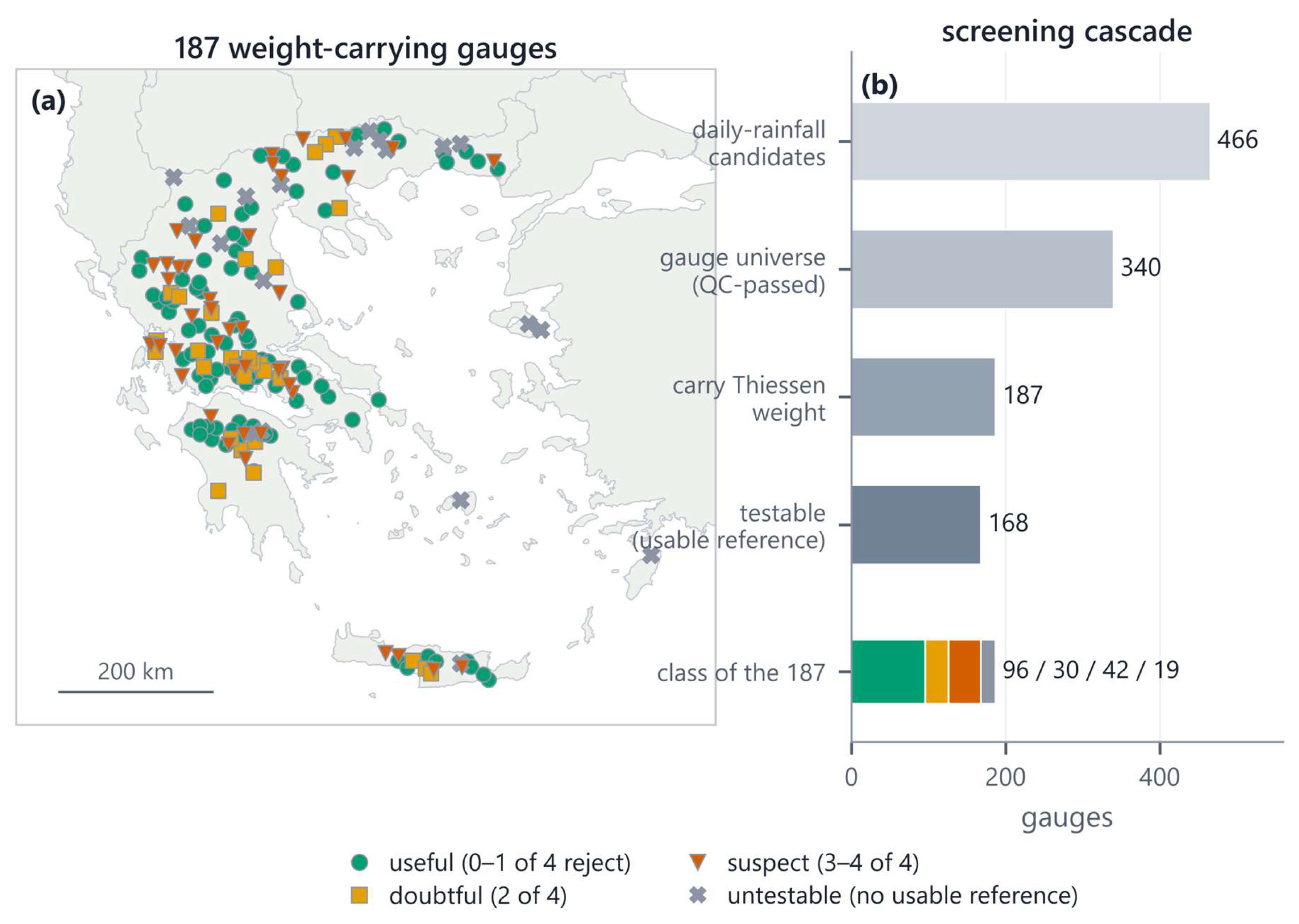
Figure 2. A worked relative-homogeneity example at the two ends of the classification: AΝΩ BΡOΝΤOΥ (suspect, all four tests rejecting) and ΠΛAΤAΝOΣ (useful, none rejecting). (a, b) Candidate annual totals and the r²-weighted composite of the five nearest admissible neighbours (grey dashed). The candidate is drawn throughout in its Figure 1 class colour — vermillion for the suspect gauge in (a, c, e), green for the useful gauge in (b, d, f) — so the single legend, placed in (b), keys the useful case; each panel title also names its gauge’s class. (c, d) The neighbour-ratio series with the SNHT-located split; horizontal rules are segment means, drawn in full ink only where the test rejects — in (d) they mark the best candidate split of a series that rejects no test. (e, f) Double-mass plots with the objective two-segment least-squares fit (solid before, dashed after the break). The suspect gauge steps from a ratio segment mean of 0.84 to 1.28 at 1998 with a double-mass slope ratio of 1.366; the useful gauge tracks its composite throughout at a slope ratio of 0.968. The break year annotated in (e, f) is located by the two-segment least-squares fit on the cumulative series and is a different estimator from the SNHT split in (c, d), so the two need not coincide: at AΝΩ BΡOΝΤOΥ they differ by two years, 1996 against 1998.

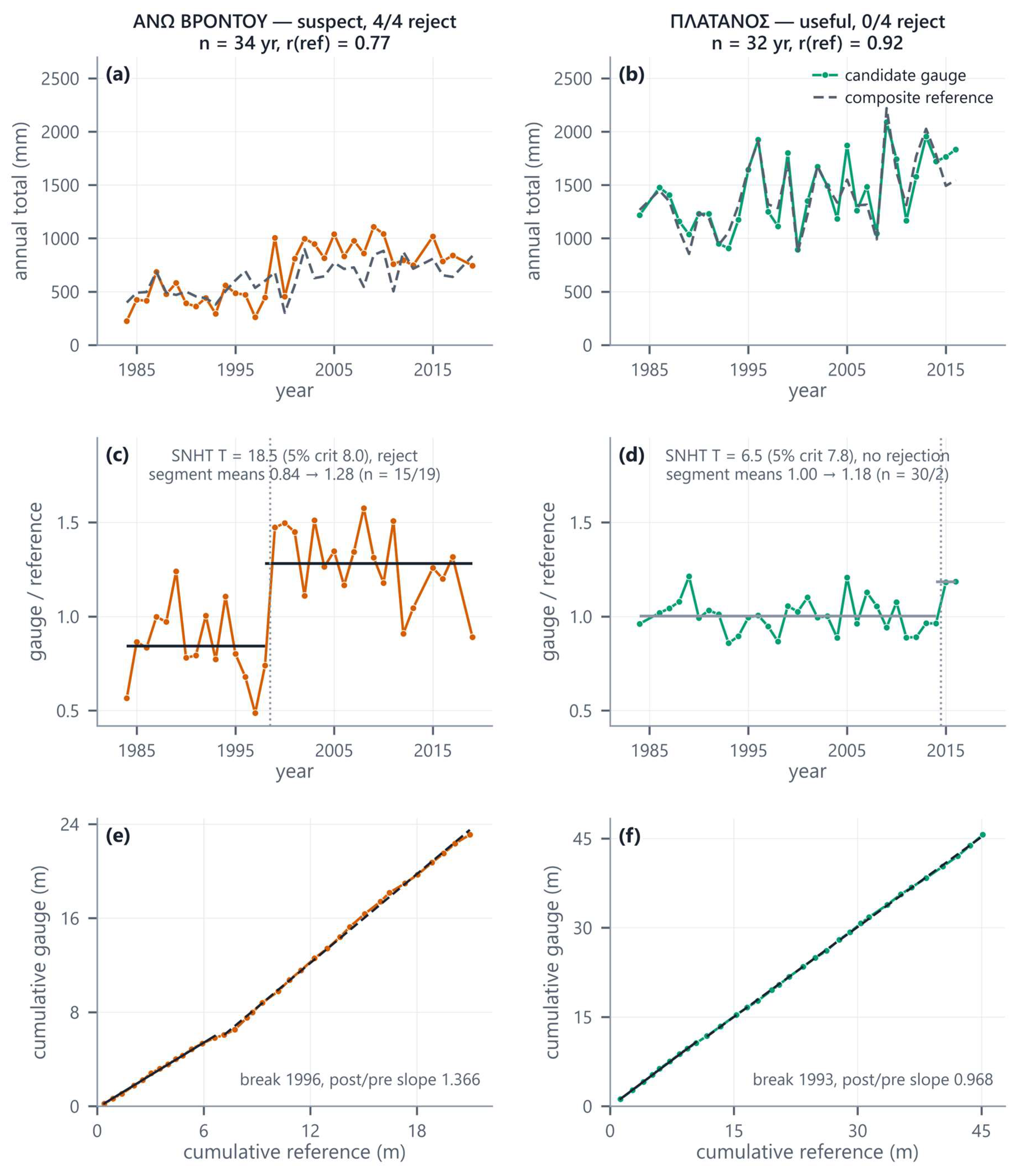
Figure 3. The relative verdict is not the absolute verdict. (a) Located Pettitt break years for gauges rejecting at 5%, from the absolute battery run on the candidates’ own series (grey) and from the relative battery run on the neighbour-ratio series (orange), on identical gauges and identical years; the shaded band marks 1995–2004. The absolute test rejects more often (70 versus 49 gauges) but its breaks are more diffuse in time (27/70 versus 30/49 inside the band). (b) Contingency of the two classifications over the 168 tested gauges: they agree for 87, while 20 absolute-suspect gauges are relative-useful and 19 absolute-useful gauges are relative-suspect.

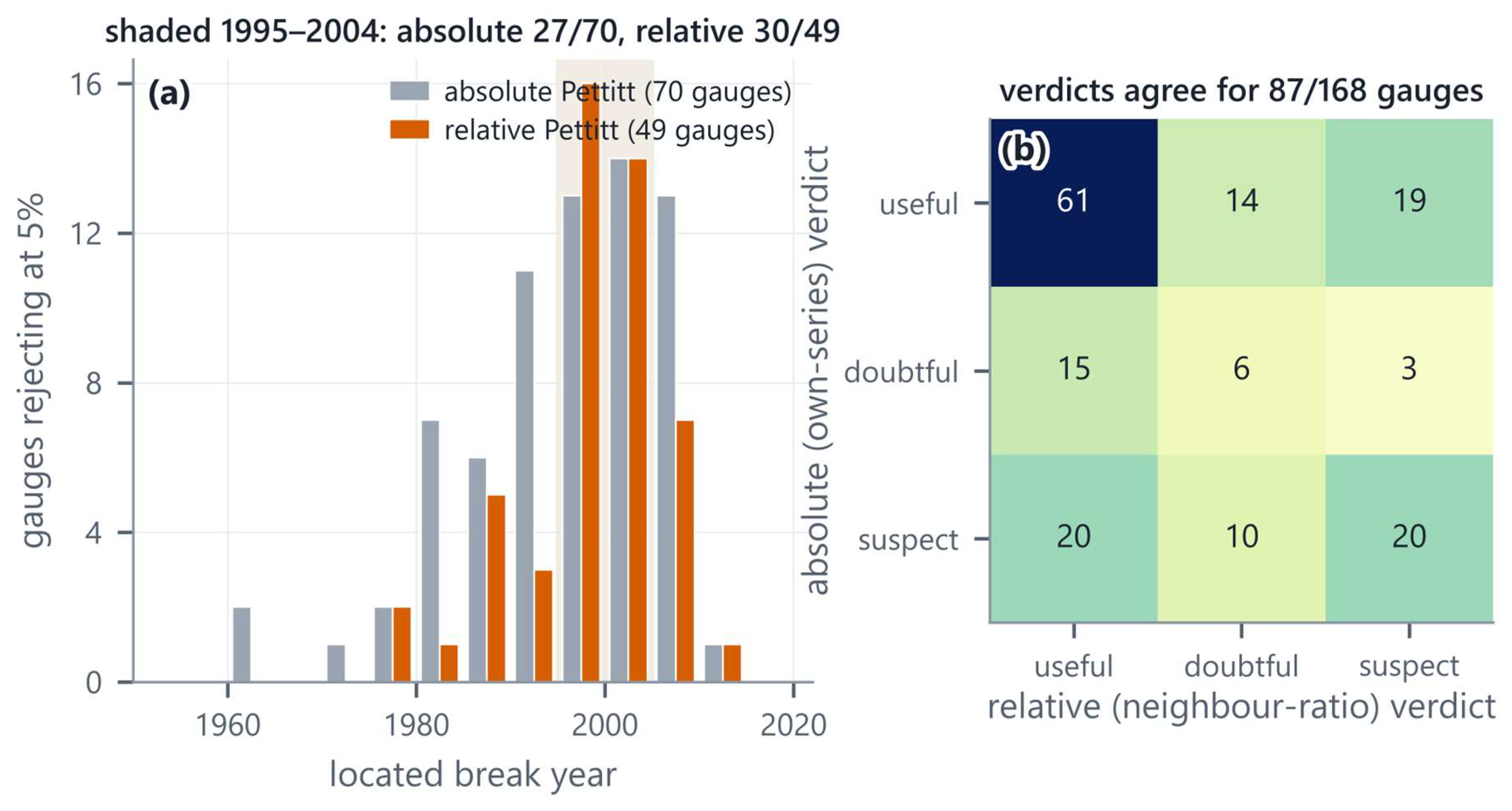
Figure 6. The artefact a homogeneity screen cannot see: EL13 Aposelemi, the only field-significant decrease in the trend family. (a) The five weighted gauge records and the resulting areal series; the two wettest gauges terminate in 1994 and 2000. (b) Per-year renormalized (realized) Thiessen weight, stacked; after 2001 the areal estimate collapses onto the drier residual gauges and from 2012 onto ΚAΛAMAΥΚA alone. (c) Static Thiessen weight against realized weight averaged over the 35 catchment-years, with each gauge’s mean annual total beneath its name. ΚAΛAMAΥΚA’s realized weight of 0.367 is 17.3 times its static weight of 0.0212 (0.021 to three decimals). The catchment mean falls from 898 mm (1984–2000) to 576 mm (2001–2018) while ΚAΛAMAΥΚA’s own record trends at only −45.4 mm decade⁻¹ (p = 0.096).

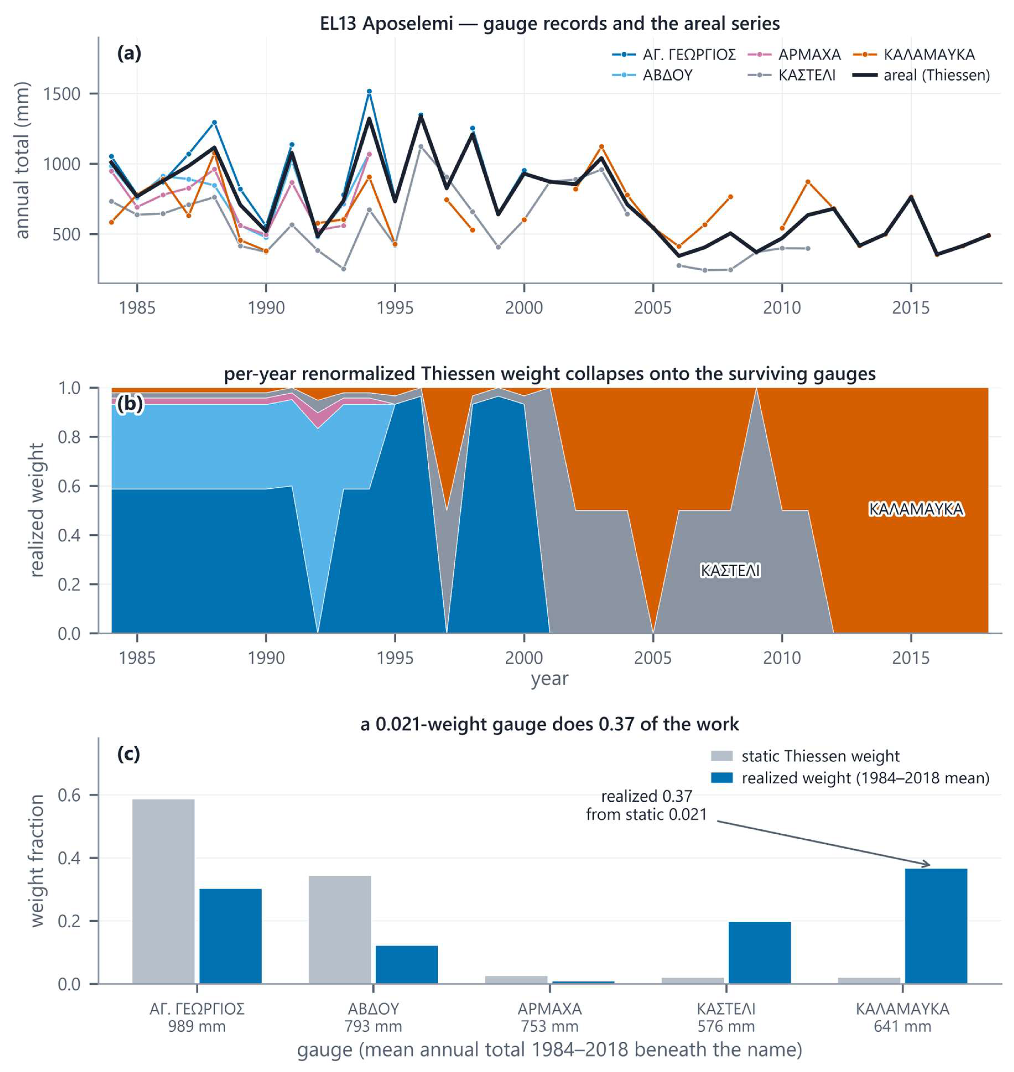
Table 1. From the daily-rainfall archive to a testable gauge population. Counts are produced by the screening code and are re-derived in the figure script. Each untestable gauge is attributed here to the gate that blocked the deepest reference tier it reached. The four-way subdivision below is finer than the deposited untestable-reason field, which carries three values (too few neighbours 9, reference correlation below 0.70 7, short record 3): that field’s correlation label is a residual bucket assigned after every neighbour tier has failed, so it also absorbs the one gauge whose composite never reached 20 paired years and for which no composite correlation exists. Its 7 is the 6 and the 1 tabulated here.

Stage	Rule	Dropped	Remaining
Candidate daily-rainfall series	daily, rainfall, coordinates present, length pre-filter, mm units, no duration series	—	466
Value-based completeness	≥ 10 years with ≥ 340 real daily values	101	365
Record quality (meteorological-service subset)	≥ 25 valid years, mean annual total 150–2,500 mm, first valid year ≤ 1990	25	340
Co-located de-duplication	rounded projected coordinates, keep most valid years	0	340 (gauge universe)
Carry Thiessen weight	non-zero weight in ≥ 1 of the 73 catchments	153	187 (screened population)
Usable neighbour reference	≥ 3 neighbours, ≥ 20 test years, r(candidate, composite) ≥ 0.70	19	168 (tested)
of which untestable: too few neighbours		9
of which untestable: reference correlation < 0.70		6
of which untestable: fewer than 20 years with both candidate and reference		1
of which untestable: record too short		3

Table 2. The four tests, their Monte-Carlo 5% critical values at two representative series lengths, and the unit-test outcome for each. Critical values are simulated from 20,000 i.i.d. standard-normal replicates per length; unit tests use 4,000 replicates at n = 36. At that replicate count the binomial Monte-Carlo standard error is ±0.0034 on a size near the nominal 5% and up to ±0.0074 on the powers, so the four sizes are individually consistent with 5% and mutually indistinguishable; the last two digits of each entry are reported for reproducibility of the fixed-seed run, not as a resolved difference.

Test	Statistic	Rejection region	5% crit., n = 30	5% crit., n = 36	Size at 5% (i.i.d. null)	Power vs +1.5 sd step
SNHT [14]	T₀ = max_k [k z̄₁² + (n−k) z̄₂²]	upper	7.747	8.011	0.0462	0.9417
Buishand range [18]	R/√n, R = range of rescaled adjusted partial sums	upper	1.494	1.522	0.0537	0.9320
Pettitt [19]	K = max_k \|U_k\|, U_k = 2R_k − k(n+1)	upper	119	159	0.0508	0.9698
von Neumann [20]	N = Σ(x_i − x_i+1)² / Σ(x_i − x̄)²	lower	1.419	1.467	0.0493	0.6820

Additional unit-test outcomes (all PASS): median located first-segment size 18 of 36 for all three locating tests; a noiseless 100 → 160 mm step between 2001 and 2002 gives 4/4 rejections and the correct located year in all three locating tests (a located break year is reported throughout as the last year of the first segment, here 2001); a single homogeneous realization gives 0 rejections; simulated von Neumann null moments 2.0016 / 0.1034 against the analytic 2 / 0.1050; the fast rank-identity Pettitt implementation agrees with an independent reference implementation on the break index in 200/200 series and on the statistic in 141/141 recoverable cases.

Table 3. The distributional axis of the null (Section 4.5), the counterpart to Table 5’s serial axis. Series are drawn i.i.d. from a lognormal marginal and tested against the published Gaussian critical values, so each row is the size the primary layer actually achieves when the ratio series is skewed rather than Gaussian. All four statistics are invariant to location, scale and reflection, so only the shape of the marginal matters and one ladder covers both tails; the generator is calibrated so that its median sample skewness at the given length equals the target, because the observed values are themselves sample estimates at a median length of 30 and the sample skewness is strongly biased toward zero in short heavy-tailed records. Lengths, replicate count (50,000) and nominal level match Table 5 exactly. The skewness = 0 row is a control and reproduces both the nominal 5% marginal size and the published 0.020 combined-rule size.

Ratio-series skewness	SNHT	Buishand	Pettitt	von Neumann	combined rule: suspect	3-of-3 locating	expected false suspects of 168
0.000 (control)	0.049	0.051	0.048	0.051	0.020	0.015	3.4
+0.272 (observed median)	0.054	0.050	0.050	0.052	0.020	0.015	3.3
+0.677 (observed upper quartile)	0.069	0.047	0.048	0.052	0.020	0.014	3.3
+1.500	0.105	0.037	0.048	0.056	0.015	0.009	2.6
+3.000 (observed maximum, 3.455)	0.154	0.018	0.048	0.069	0.009	0.003	1.5

Monte-Carlo precision, and the classification under a skewed null: At n = 30, Monte-Carlo standard errors 0.001 on the marginals and 0.0004 to 0.0006 on the combined rule. The final column is 168 times the unrounded combined-rule rate, so it will not always reproduce from the three-decimal rate displayed beside it. Pettitt is flat across the whole ladder, as a rank-based test must be. SNHT is inflated and Buishand deflated by skewness, in opposite directions and by comparable amounts, so the three-of-four count — which requires the tests to agree — is not mis-sized at any observed skewness and is conservative beyond it. Re-running the whole battery with a null built at every gauge’s own length and own fitted skewness moves the classification from 96 / 30 / 42 to 99 / 29 / 40, with 7 of 168 gauges changing class; a control run of the identical path at skewness 0 returns 95 / 32 / 41 rather than the published 96 / 30 / 42, so the movement is of the same order as the Monte-Carlo redraw noise of the null itself. The 7 moves are 6 to 1 toward the less suspect end — 4 doubtful gauges become useful and 2 suspect ones doubtful, against 1 useful gauge becoming doubtful, and no gauge crosses from useful to suspect or back — and the two classifications agree for 161 of 168 at κ = 0.93, against 87 of 168 at κ = 0.17 for the relative-versus-absolute comparison of Section 3.1. That net direction is not itself evidence, because the zero-skew control moves too, and by a comparable amount in the opposite direction. Unlike Table 5, this table carries no “of the 16” column of its own: the field verdict for every recalibrated axis, this one included, is collected in Table 6.

Table 4. The 18 screening combinations. n is the retained family size; “raw” and “BH” are counts of significant increases/decreases before and after Benjamini–Hochberg control at q = 0.05 applied within the retained family; “rate” is raw increases divided by n; “of the 16” is how many of the unscreened field-significant increases survive. Unscreened reference: n = 71, raw 30/1, BH 16/1, rate 0.423, median +54.2 mm decade⁻¹.

Scenario	Threshold	n	Dropped	raw ↑/↓	BH ↑/↓	rate	median (mm dec⁻¹)	of the 16
A — realized suspect weight (primary)	0.00	30	41	12/0	8/0	0.400	+48.3	8
A	0.25	45	26	20/1	13/1	0.444	+57.0	13
A	0.50	55	16	23/1	13/1	0.418	+48.8	13
B — suspect + untestable	0.00	16	55	9/0	6/0	0.563	+81.3	6
B	0.25	30	41	17/1	14/1	0.567	+88.4	13
B	0.50	42	29	21/1	13/1	0.500	+70.6	13
C — suspect + doubtful	0.00	22	49	5/0	3/0	0.227	+36.4	3
C	0.25	30	41	9/1	7/1	0.300	+38.0	7
C	0.50	42	29	16/1	9/1	0.381	+42.9	9
D — worst of ratio/difference	0.00	28	43	11/0	8/0	0.393	+48.3	8
D	0.25	40	31	16/1	13/1	0.400	+61.3	13
D	0.50	53	18	22/1	13/1	0.415	+48.8	13
E — suspect only if break in window	0.00	30	41	12/0	8/0	0.400	+48.3	8
E	0.25	48	23	21/1	13/1	0.438	+52.2	13
E	0.50	57	14	23/1	13/1	0.404	+50.2	13
F — static weights, suspect	0.00	30	41	12/0	8/0	0.400	+48.3	8
F	0.25	49	22	22/1	13/1	0.449	+54.2	13
F	0.50	57	14	25/1	13/1	0.439	+50.2	13

Table 10. The layer-two amplification diagnostic re-run on the reconstructions the screen itself creates (Section 3.7). For every rule the dominant surviving gauge’s realized weight — the per-year renormalized share averaged over the catchment-years the catchment reports — is compared with its static Thiessen share, under two reference points. Against the survivors renormalizes the static share over the gauges that remain, which is the published diagnostic’s own recipe transplanted onto the reduced support; it measures the network’s mortality schedule. Against the original network divides the same realized share by the gauge’s static share in the full published network; it is the only one of the two that can see the deletion, because a catchment reduced to a single surviving gauge scores exactly 1.0 against the survivors by construction, however small that gauge’s share of the original network was. L0 is the fail-closed parity row: deleting nothing must reproduce the published count of 7 amplified catchments in the trend family (8 of all 73), and the run aborts if it does not.

Rule	n reconstructible	> 2× vs survivors	> 2× vs original network	max vs original	at	of the 16 amplified vs original
L0 — delete nothing (parity)	71	7	7	17.3	EL13_APOSELEMI	4
L1 — suspect (primary)	66	5	16	19.4	EL12_ESYMI	7
L2 — suspect + untestable	55	4	17	24.8	EL13_APOSELEMI	7
L3 — suspect + doubtful	62	6	24	624.9	EL11_KERKINI	8
L4 — worst of ratio / difference	65	5	15	28.7	EL11_KERKINI	7
L5 — suspect, break in window	67	5	14	19.4	EL12_ESYMI	7
L6 — multiplicity-controlled (within-test)	70	7	14	17.3	EL13_APOSELEMI	7
L7 — jointly multiplicity-controlled	70	7	14	17.3	EL13_APOSELEMI	7
L8 — recalibrated suspect (4 gauges)	71	7	8	17.3	EL13_APOSELEMI	5

The two reference points, and what each can see: Read against the survivors the reconstructions look no worse than the published product — the count falls from 7 of 71 to 5 of 66 under the primary rule, and the median amplification is exactly 1.000 under every rule. Read against the original network the primary rule more than doubles the count, from 7 to 16, and raises the median from 1.000 to 1.107; the most aggressive rule (L3) reaches 24 of 62 and concentrates EL11_KERKINI onto ΣΚΡA, a gauge holding 0.0016 of the original static weight, an amplification of 625. Of the three new detections, EL04_AMVRAKIA is itself an amplification product at 5.8× (ΛEΠEΝOΥ, 0.171 of the original network, carrying all of it); EL04_OZEROS reconstructs to the same single ΛEΠEΝOΥ series at 1.9×, so the two are one piece of evidence and not two; EL08_LIMNI_SMOKOVOU sits at 2.0×, on the line. L8 is the low end of the calibration range, added so that the new diagnostic is run at both ends of the dose–response of Section 3.6 rather than only at the high one: deleting the 4 gauges the AR(1) recalibration flags — the same four the calendar-aware recalibration flags, Table 6 — costs no catchment, leaves the against-survivors count at the published 7 and lifts the against-original count only from 7 to 8 and the of-the-16 count from 4 to 5, the one addition being EL02_ASTERIOU. The concentration the diagnostic detects is therefore a property of deleting 42 gauges, not of deleting flagged gauges as such. Rows are ordered by label; ordered by dose instead, L8 would fall second, immediately after L0.

Disclaimer/Publisher’s Note: The statements, opinions and data contained in all publications are solely those of the individual author(s) and contributor(s) and not of MDPI and/or the editor(s). MDPI and/or the editor(s) disclaim responsibility for any injury to people or property resulting from any ideas, methods, instructions or products referred to in the content.

© 2026 by the authors. Licensee MDPI, Basel, Switzerland. This article is an open access article distributed under the terms and conditions of the Creative Commons Attribution (CC BY) license (http://creativecommons.org/licenses/by/4.0/).

Copyright: This open access article is published under a Creative Commons CC BY 4.0 license, which permit the free download, distribution, and reuse, provided that the author and preprint are cited in any reuse.