
Submitted:
21 July 2026
Posted:
05 August 2026
You are already at the latest version
Abstract
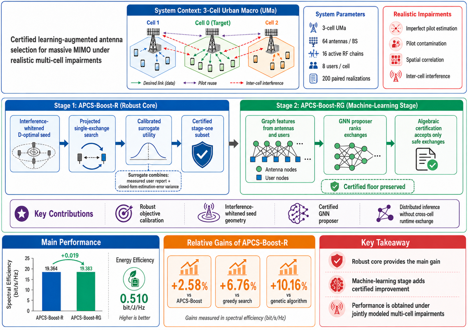
Circuit power consumed by radio frequency chains in massive multiple input multiple output arrays is reduced through antenna selection. Conventional gains are commonly established under perfect channel knowledge and isolated cell assumptions, whereas deployed links are affected jointly by estimation error, pilot contamination, spatial correlation and inter cell interference. Two complementary primary contributions are proposed. APCS Boost R provides interference calibrated algebraic selection through an interference whitened D optimal seed and projected exchanges implemented with rank one updates. Candidate subsets are evaluated by a calibrated surrogate that combines a user measurement report with a closed form estimation error correction while preserving the algebraic update structure. APCS Boost RG provides certified network informed learning through a physics derived heterogeneous graph neural network trained by imitation of a network level partial response oracle. Learned exchange potentials are combined with exact surrogate increments and every accepted subset is verified against the robust stage utility floor. In a three cell urban macro system with 64 antennas, 16 active chains and eight users per cell, APCS Boost R attains 19.364 bit/s/Hz over 200 paired realizations. Improvements of 2.58 percent over APCS Boost, 6.76 percent over norm initialized greedy search and 10.16 percent over a genetic algorithm are obtained with a selection time of 20.4 ms. Energy efficiency is increased from 0.497 to 0.510 bit/J/Hz without a statistically significant change in minimum user rate. APCS Boost RG provides an additional 0.019 bit/s/Hz, with a positive mean in every replication and a confidence interval excluding zero. The learned key produces a tighter paired interval than exact surrogate ranking within the same single exchange neighbourhood while preserving the certified floor. The results demonstrate that objective calibration and certified graph learning provide complementary gains under jointly modelled multi cell impairments with distributed inference and no runtime cross cell signalling.
Keywords:
massive MIMO
; antenna selection
; machine learning
; 3GPP TR 38.901
; imperfect channel estimation
; pilot contamination
; spatial correlation
; multi-cell interference
; energy efficiency
; graph neural networks
1. Introduction
In massive multiple-input multiple-output (MIMO) systems, a large base-station array is used to spatially multiplex many users on the same time-frequency resource [1,2]. The array gain can increase spectral efficiency and reduce the radiated energy required per information bit [3]. In a fully digital array, each active antenna is nevertheless associated with a radio-frequency (RF) chain, a converter pair, a filtering path and a baseband-processing load. Circuit power can therefore move the energy-efficient operating point away from the maximum-array operating point [4]. This issue is addressed through antenna selection, in which a smaller RF-chain pool is connected to a larger physical array. It has also been confirmed through measurement campaigns that the physical antennas of a large array do not contribute equally [5].
The resulting subset problem is combinatorial. Selecting antennas from candidates produces approximately possible subsets. Norm-based ranking is inexpensive but ignores inter-column dependence. Stronger subsets can be provided by greedy search and genetic-algorithm (GA) search, although repeated complete zero-forcing (ZF) evaluations increase selection latency [6,7,8]. Part of the computational burden can be transferred offline through learning-based methods, but generalization may be impaired by incomplete channel state information (CSI) and changes in the propagation distribution [9,10,11].
A central challenge is that antenna-selection results are often established under independent Rayleigh fading and perfect CSI. Practical cellular links are affected by distance-dependent attenuation, line-of-sight transitions, shadow fading and angular concentration. CSI is obtained from finite-power pilots and coherent contamination across cells is created by pilot reuse. Additional interference is produced by downlink signals from neighbouring base stations. Spatial correlation is not merely a nuisance because its covariance structure can sometimes be exploited, but it changes the rank and conditioning of the selected channel [12,13]. The effect of the selector must therefore be separated from the effects of channel estimation and interference in a credible assessment.
The study is motivated by the interaction between the selector objective and the impairments applied during evaluation. When a selection method is developed under perfect CSI and isolated-cell operation, those assumptions are inherited by its internal objective even when they are not adopted in the evaluation. The diagnostic study reported in Section 4.2 shows that direct refinement of the achieved rate exposes substantial improvement, whereas replacing the estimated search input with the true channel alone does not. Objective calibration is therefore identified as the principal opportunity beyond increased search effort.
APCS-Boost is defined in this work as the uncalibrated algebraic baseline formed by the initialization and exchange procedures of Section 4.1. Throughout the paper, the suffix R denotes the interference-calibrated algebraic stage, the suffix G denotes the certified graph learning stage, RG denotes their integration and EE denotes the adaptive energy-efficiency mode. Two primary contributions are developed. First, the surrogate objective and the D-optimal seed are calibrated to measured interference and estimated-channel conditions within a three-cell system-level examination derived from 3GPP TR 38.901 [14]. Second, network-level learned exchange information is integrated through a physics-derived graph neural network whose proposals are accepted only after algebraic certification.
The proposed framework is distinguished within multi-cell antenna selection by the joint treatment of pilot error, pilot contamination, spatial correlation and inter-cell interference in a common 3GPP-derived layout. The external state-of-the-art comparison in Table 1 covers thirteen external approach families represented by fourteen published studies spanning energy-efficient ranking, genetic and graph search, supervised and unsupervised deep learning, incomplete-CSI optimization, learned transmitter configuration and certified neural selection. The internal APCS stages are not counted as external comparators and are evaluated separately through controlled ablations. The algebraic contribution is formed by the interference-calibrated surrogate and whitened D-optimal geometry. The machine learning contribution is formed by network-level partial-response labels, graph-based residual exchange ranking and a calibrated stage-one utility floor within the same multi-cell selection framework. Under the adopted rule, the certified surrogate utility is preserved at or above the robust stage-one value. Exact surrogate ranking is included as a controlled attribution reference for the learned residual key.
The contributions are as follows.
- 1.
- The antenna-selection problem is reformulated for estimated multi-cell channels. Selection is performed on , while actual downlink rates are computed from the true channel and include residual intra-cell leakage and inter-cell interference. Reported gains therefore correspond to rates measured on the simulated true channels under the stated assumptions.
- 2.
- A diagnosis is performed that separates search quality from objective quality and attributes the residual gap of APCS-Boost to the surrogate rather than to the neighbourhood. An achieved-rate hill climb started from APCS-Boost reveals approximately 6% improvement within the diagnostic budget, which confirms substantial objective headroom.
- 3.
- APCS-Boost-R, the interference-calibrated algebraic contribution, is developed. The per-user surrogate SINR is divided by an effective noise term that combines a measured interference-plus-noise report with a closed-form estimation-error correction available from large-scale gains, the pilot map and the pilot SNR. The D-optimal seed is additionally constructed on the interference-whitened estimate. Both corrections are per-user scalars, so the rank-one exchange machinery and its complexity order are preserved. Under the joint impairments, 19.364 bit/s/Hz is achieved by APCS-Boost-R, exceeding APCS-Boost by 2.58%, greedy search by 6.76% and GA by 10.16% at a selection time of 20.4 ms.
- 4.
- An ablation is reported in which the identical surrogate is supplied to greedy and genetic search. The residual advantage of APCS-Boost-R is thereby attributed to the whitened seed geometry rather than to the additional information alone. Approximately 1% is recovered by either baseline, so roughly three fifths of the advantage is supplied by the whitened seed.
- 5.
- APCS-Boost-RG, the certified machine learning contribution, is developed. A physics-derived heterogeneous graph neural network is trained by imitation of a network-level partial-response oracle and is used to rank exchanges. Every accepted proposal is validated against the calibrated algebraic surrogate, so the final certified utility is preserved at or above the APCS-Boost-R stage-one value. A statistically significant additional gain is obtained and a tighter paired interval is produced than by exact surrogate ranking within the complete single-exchange neighbourhood. The ablations demonstrate the value of network-level labels and the protection supplied by the verifier.
- 6.
- The joint stress comparison is obtained from five independent replications of 40 paired realizations, while each controlled sweep uses five replications of 20 paired realizations. Across-replication spread is reported so that the stability of the ranking can be judged.
The remainder of the paper is organized as follows. Section 2 reviews antenna selection, imperfect CSI, standardized channels and learning-augmented optimization and positions the proposed approach in Table 1. Section 3 presents the three-cell system, the channel layer, the pilot-based estimator and the transmission objective. Section 4 develops the proposed approach in stages: the D-optimal initialization, the projection and exchange machinery, the diagnosis that motivates the calibrated surrogate, the robust core APCS-Boost-R, the machine-learning stage of APCS-Boost-RG with its training and certification, the adaptive chain mode with the complexity analysis and the overall execution in Algorithm 2. Section 5 reports the protocol, the joint stress comparison, the attribution ablation, the learned-stage results with their variant examination, the replication stability, the single-impairment sweeps and the evaluation scope. Section 6 concludes the paper and outlines future work.
2. Literature Review and Background Work
This section reviews representative recent antenna-selection methods, learning-based selectors, incomplete-CSI formulations and standardized channel models. The external literature is compared with the proposed framework and the specific gap addressed by the present study is then identified.
2.1. RF-Chain Activation and Antenna Selection
In this subsection, the antenna-selection literature relevant to RF-chain power is reviewed. The energy efficiency of a massive-MIMO base station depends on the transmit power, active array size, user load and processing architecture [3,4]. Received-power ranking and energy-aware subset selection have been used to retain array gain while reducing RF-chain power [6,15]. Genetic and quasi-distributed search have been developed for extra-large arrays [7], while exact graph search has been investigated for moderate dimensions [8]. Joint antenna selection and precoding has also been addressed through low-complexity heuristic optimization [16]. More recent formulations have incorporated incomplete CSI through a risk-aware constraint [10]. These studies establish strong optimization foundations, although joint evaluation under pilot error, pilot contamination, spatial correlation and downlink inter-cell interference is not provided within a common 3GPP-derived setting.
2.2. Imperfect CSI and Pilot Contamination
In this subsection, the prior work on estimation error and pilot contamination is summarized. In time-division duplex systems, uplink pilots are used to infer downlink channels through reciprocity. The number of mutually orthogonal pilots is limited by the coherence interval. When pilots are reused across cells, the estimate of a desired user is contaminated by channel components from pilot-sharing users [1]. Pilot contamination is not necessarily an asymptotic capacity limit when covariance matrices are sufficiently distinct and appropriate processing is available [12]. It remains a finite-dimensional concern for ZF precoding because residual intra-cell leakage and misdirected beams are produced by an inaccurate estimate. Antenna selection under incomplete CSI has recently been treated through risk-aware optimization [10], while correlated-channel capacity approximations have shown that estimation error and spatial dependence must be considered jointly [13]. The approach adopted here differs in that the uncertainty is not carried as a distributional risk constraint but is condensed into a per-user scalar that leaves the algebraic update structure of the search intact.
2.3. 3GPP Spatial Channels and Research Gap
In this subsection, the standardized channel framework is introduced and the research gap is stated. Channel-model components for frequencies from 0.5 to 100 GHz are defined in 3GPP TR 38.901, including deployment scenarios, LOS probabilities, distance-dependent path loss, shadow fading, spatial consistency and link-level TDL/CDL models [14]. Its UMa model is appropriate for a macro-cell examination at 3.5 GHz. A narrowband spatial realization of the standardized UMa large-scale equations and geometry is used in the evaluation. The research gap addressed is the absence of a unified antenna-selection examination in which imperfect estimation, pilot reuse, angular concentration and downlink multi-cell interference are introduced separately and then jointly under a common 3GPP-derived layout, together with a selection objective that is calibrated to those impairments rather than assumed away.
2.4. Learning-Augmented Selection
In this subsection, state-of-the-art learning-based antenna selection is reviewed and the proposed machine learning contribution is positioned against it. Convolutional and deep neural networks have been used for joint antenna selection and hybrid beamforming [17,18], while multi-label learning has been used to predict massive-MIMO antenna subsets directly [9]. Label-free joint selection and beamforming has been developed through deep unsupervised learning [19] and learned transmitter configurations have been optimized for energy-efficient massive-MIMO beamforming [20]. Boosted learned selection provides another recent low-complexity direction [21]. Certified robustness has also been studied for neural antenna selectors under bounded input perturbations [22]. In cell-free MIMO, distributed convolutional antenna selection and graph-based precoding have been combined using locally estimated CSI [11].
The comparison in Table 1 contains thirteen external approach families represented by fourteen state-of-the-art studies and one row for the complete proposed framework. Internal stages such as APCS-Boost, APCS-Boost-R and the controlled APCS-Boost-RG variants are deliberately excluded as independent literature comparators because they belong to the same framework. The comparison is methodological because the cited studies use different array dimensions, channel models, precoders, power models and optimization objectives. Direct numerical evaluation is therefore performed only for baseline families that are reimplemented under the identical three-cell model and common realizations in Section 5. Within the external literature summarized in Table 1, the present framework is distinguished by the combination of estimated multi-cell CSI, jointly modelled 3GPP-derived impairments, network-informed graph proposals and a certified calibrated-surrogate floor.
3. System Description and Problem Formulation
This section provides the three-cell downlink model, the 3GPP-derived channel construction, the pilot-based channel estimator, the true-channel transmission metrics and the surrogate antenna-selection objective. The assumptions and notation used by the proposed algorithms are defined before the methodology is introduced.
3.1. Three-Cell Downlink Architecture
In this subsection, the network layout and the notation are defined. A time-division duplex network with cells is considered. At each base station, M physical antennas are deployed, of which a subset is connected to active RF chains. In each cell, K single-antenna users are served. The serving cell is indexed by , while denotes the neighbouring cells. The base stations are separated by an inter-site distance of 500 m. User locations are sampled independently at distances between 35 m and 220 m from the serving base station. The processing and interference paths are illustrated in Figure 1. The principal symbols used throughout the paper are collected in Appendix B, while the abbreviations are expanded in the list at the end of the paper.
Let denote the channel from base station b to user k in cell c. Here b indexes the transmitting base station and c indexes the cell in which the served user resides, so the central desired link corresponds to while cross-cell interference contributions have . The corresponding matrix is
The central-cell users are considered in the analysis, but the local channels are independently estimated at every base station, after which antennas are selected and a precoder is formed.
3.2. 3GPP TR 38.901-Derived Channel Layer
In this subsection, the large-scale and small-scale channel construction is described. For each BS-user link entering Equation (1), the three-dimensional distance is
The UMa LOS probability is applied as specified by TR 38.901 and is evaluated with the two-dimensional distance . For the adopted user height m, the height-correction term becomes zero, so Equation (3) is obtained:
For a carrier frequency expressed in GHz, the LOS path loss before the breakpoint is obtained using the three-dimensional distance defined in Equation (2) as
while the post-breakpoint expression is
The breakpoint distance is defined as with the carrier frequency expressed in Hz, the speed of light c and the effective heights m and m. The NLOS candidate is
The final NLOS loss is selected as the maximum of the applicable LOS value from Equation (4) and Equation (5) and the NLOS candidate in Equation (6). Continuity at the breakpoint is thereby preserved. Log-normal shadow fading with standard deviations of 4 dB for LOS links and 6 dB for NLOS links is added.
In the default small-scale backend, rays are used. Their departure angles are drawn from a Laplace distribution around the geometric BS-user direction with configurable azimuth angular spread (ASD). For a half-wavelength uniform linear array, the steering vector is
The NLOS channel is a weighted sum of the steering vectors in Equation (7). A 9 dB Rician component is included for LOS links. The standardized UMa large-scale ratios are preserved by this construction while a controlled spatial-correlation parameter is provided. The adopted channel layer is a narrowband system-level realization. Complete delay, polarization and mobility procedures are outside the scope of the present model.
3.3. Pilot-Based Channel Estimation
In this subsection, the pilot protocol and the estimator are specified. Within each cell, K orthogonal pilots are assigned. The cells in which the same pilot set is reused are determined by a cell-level reuse factor . After the received pilot signal is correlated with the pilot of user k, the normalized observation at base station b is obtained as
where contains the cells sharing the same pilot group. The reuse factor sets the number of distinct pilot groups formed across the cells, so cell c is assigned to pilot group . A factor of one therefore places all cells in one shared group, a factor of three assigns a unique group to each cell. For the three-cell layout, a factor of two places the serving cell and neighbour cell 2 in a shared group while neighbour cell 1 uses an orthogonal group. Two cells are contaminating whenever they share a group index. The pilot noise is modelled as zero-mean circularly symmetric complex Gaussian. With the normalization applied in Equation (8) its per-antenna variance equals , so is the pilot SNR referenced to the desired large-scale gain. With the large-scale coefficient , the adopted scalar LMMSE-like shrinkage is
where the shrinkage coefficient is retained explicitly because it is reused in Section 4.3. The normalized mean-square error is
Perfect CSI is represented by and a reuse factor that assigns a unique pilot group to every simulated cell.
3.4. ZF Transmission and Selection Objective
In this subsection, the precoder, the achieved-rate metrics and the selection objective are defined. Given a subset , normalized ZF is formed from the estimated subchannel:
Each column of Equation (11) is then normalized to unit norm, where is a numerical regularization term. The actual SINR of central-cell user k is
where
The intra-cell term of Equation (13) and the inter-cell term of Equation (14) enter Equation (12) together with the true channels. Neighbouring-cell load is controlled by the activity factor , while p denotes the normalized data-transmit SNR. The rate is , the sum rate is and Jain fairness [23] is
The central-cell power model is
and energy efficiency is defined as , where is given by Equation (16).
The true rates above are not available to the selector. The estimated channel is used to maximize the surrogate utility
in which the sum rate , the minimum rate and the Jain index J are evaluated on the surrogate SINRs of the estimated ZF solution and is a normalization reference value with the mean per-user noise of the surrogate in use. The maximization of Equation (17) is performed under the fixed cardinality , full user rank and the per-user channel-energy coverage constraint, while the user-rate floor bit/s/Hz enters as the capped soft term of Equation (17) and the spectral condition-number limit is evaluated at the final subset, where denotes the ratio of the largest to the smallest eigenvalue of the estimated subchannel Gram matrix and . If the final validation fails, the feasible stage-one seed is returned. The selected subset is deliberately evaluated on the true multi-cell channel, so estimation and interference losses are not concealed within the objective.
4. Methodology
This section presents the complete proposed framework. The algebraic initialization and projected exchange procedure are first defined, the objective mismatch is then diagnosed, the interference-calibrated robust stage is developed and the certified graph learning stage is integrated with the algebraic verifier.
4.1. Algebraic Initialization, Projections and Exchanges
In this subsection, the algebraic machinery of the selector is presented: the seed construction, the projection and shortlist rule and the rank-one exchange step. For a given base station, estimated channel column m is denoted by . The regularized information matrix of subset is
where regularizes Equation (18). The incremental log-determinant gain is maximized by a D-optimal seed. For a candidate antenna m, the matrix determinant lemma [24] is used to obtain
Users for whom substantial energy has already been accumulated can be overemphasized by a determinant-only seed. Therefore, the selected energy of user k is maintained by APCS-Boost as
and is compared with the total available energy . The weak-user weight is computed as and is normalized to unit mean across the users, so Equation (20) drives the coverage pressure. The array is also divided into four aperture blocks, where denotes the block containing antenna m. The score is
with and . When the number of remaining slots equals the number of uncovered blocks, only antennas from uncovered blocks are eligible. After insertion, the inverse is updated by
The seed is deterministic and requires no population initialization or training data.
The projection machinery and the shortlist rule are presented next. The completed seed is screened before refinement. It must contain at least one selected antenna in every aperture block and must satisfy
where and the coverage energy of Equation (20) is evaluated on the raw estimated channel rather than on the whitened energy used for seed scoring. The removal of an excessive share of the selected channel energy from a weak user during a swap is prevented by the projection in Equation (23). Candidates that produce a nonpositive inverse-downdate denominator are rejected because the resulting matrix would approach rank deficiency.
The leverage of selected antenna i is
Only the selected antennas with the smallest leverage are considered for removal. They contribute the least unique information under the current inverse and are the most plausible replacement candidates. The neighbourhood is thereby reduced from to exchanges per round.
The exchange step and its low-rank updates complete the machinery. Let denote the inverse Gram matrix of the current estimated subchannel. Removing selected antenna i gives
For an outside antenna j, the vector is defined. The candidate inverse is
Equal-power estimated ZF rates only require . All feasible outside antennas for a fixed removal are therefore evaluated in one vectorized update. The candidate with the largest strictly positive utility increment is accepted. Each accepted exchange increases the surrogate utility, so cycling is impossible. One complete ZF solution and one condition-number check are performed for the final subset. If the final validation fails, the feasible stage-one seed is returned.
4.2. Diagnosis: The Objective Rather Than the Search
In this subsection, the experiment that attributes the residual gap to the surrogate objective is reported. The surrogate used above assigns to user k the estimated SINR
Two assumptions are embedded in Equation (27). The denominator of the true SINR is replaced by unity, so interference is treated as absent. In addition, is treated as exact, so estimation error is treated as absent. Neither assumption holds at the operating point examined in Section 5, where a mean NMSE of 0.107 is measured.
Two controlled diagnostics were performed at the joint stress point to determine whether the residual gap was caused by the neighbourhood or by the objective. In the first diagnostic, selection was repeated with the true channel supplied to the selector instead of the estimate. No improvement in the achieved sum rate was observed, which indicates that estimation noise in the search input was not the binding constraint. In the second diagnostic, hill-climbing was performed directly on the own-cell achieved sum rate from the APCS-Boost subset. A gain of approximately 6% was obtained before the non-converged procedure was stopped. This value is a partial diagnostic trajectory rather than an upper bound. The 21.6% per-cell and 7.2% network figures reported later are produced by different oracle objectives, both started from APCS-Boost-R and are therefore not directly comparable with the 6% diagnostic. The three definitions are summarized in Table 2. Substantial headroom is present within the exchange neighbourhood, but it is not exposed by the uncalibrated surrogate. It was therefore concluded that APCS-Boost is limited by its objective rather than by the availability of candidate exchanges.
4.3. APCS-Boost-R: Interference-Calibrated Selection with an Estimation-Error Correction
In this subsection, the calibrated robust surrogate and the whitened seed that form the algebraic core of the proposed approach are developed. In APCS-Boost-R, Equation (27) is replaced by
where the effective noise of user k is
The measurement-based term and the analytic estimation-error term are defined below.
The term represents the interference plus noise experienced by user k. It is measured at the user equipment under a sounding configuration and is returned through a standard measurement report. Because the report reflects residual intra-cell leakage, partial overlap with the analytic error term of Equation (31) is possible. The two components are therefore interpreted as complementary calibration signals rather than as a disjoint decomposition. A paired ablation over 100 joint-stress scenes is reported in Section 5.2.1. The measured report captures experienced interference directly, while the analytic term introduces explicit pilot-estimation dependence from quantities available at the base station. Cross-cell channel knowledge, covariance exchange and backhaul coordination are not required. The sounding configuration is taken to be the coverage-aware D-optimal seed of Section 4, which is already computed and therefore adds no search cost.
The term is the per-antenna variance of the estimation error of user k. From Equation (8) and Equation (9), the error is
whose per-antenna variance is obtained from Equation (30) in closed form as
Only large-scale gains, the pilot map and the pilot SNR are included in Equation (31). Equation (31) is exact for uncorrelated channel entries and is used as a per-user scalar approximation under the correlated and Rician channels of Section 3. The approximation is retained as an auxiliary estimation-error correction and its contribution is examined through the decomposition ablation of Section 5.2.1. All three quantities are available at the base station, so no additional signalling is introduced. Residual intra-cell leakage across the interfering streams, which is produced by an erroneous estimate, is represented by the factor in Equation (29).
The essential property of Equation (28) is structural. Both corrections enter as a single positive per-user scalar multiplying the inverse-Gram diagonal. The quantity required by the vectorized exchange in Equation (26) therefore remains and the Sherman-Morrison downdate and update in Equation (25) and Equation (26) are unchanged. The complexity order of the refinement is consequently preserved.
The seed is also modified. Rather than applying Equation (21) to , it is applied to the interference-whitened estimate
Volume is then measured by the determinant recursion in Equation (19) and Equation (22) in a metric where each user axis is scaled by the reliability with which that user can actually be served. Aperture is thereby spent on users able to benefit from it rather than on users that are interference limited or poorly estimated. Since is diagonal and fixed within a selection, Equation (32) costs and leaves the recursion unaltered.
The refinement depth is increased from three rounds to . The deeper budget is justified in Section 5 by the observation that the calibrated surrogate continues to yield accepted exchanges beyond the third round, whereas the uncalibrated surrogate saturates. The complete robust selection procedure is summarized in Algorithm 1.
| Algorithm 1:APCS-Boost-R with Estimated Multi-Cell CSI |
Require: , , pilot map , , L, , q,
|
4.4. APCS-Boost-RG: Certified Learned Exchange Rankings
In this subsection, the certified machine learning stage is developed from the oracle analysis through graph construction, training and verified integration. A best-improvement search over the shortlisted neighbourhood is performed in APCS-Boost-R, so a surrogate-local optimum is reached within the complete combinatorial space. A simulation oracle identifies further network-level opportunity. When an achieved network sum-rate hill climb is started from the APCS-Boost-R subset with true channels, the network objective is increased by 7.2% on average. Among the beneficial oracle exchanges, 83.4% fall outside the surrogate-monotone path and the median relative surrogate reduction is 1.31%. This result establishes the need for a residual ranking signal that represents network-level information beyond the per-cell surrogate. The 7.2% network-level value is measured from the APCS-Boost-R subset and is distinct from the approximately 6% own-cell diagnostic reported for APCS-Boost in Section 4.2. Algebraic certification is retained for every accepted learned exchange.
For each cell, a heterogeneous bipartite graph is constructed from quantities available at the base station. Twelve engineered features are assigned to each of the M antenna nodes and seven are assigned to each of the K user nodes, all derived from the physical quantities of Section 3 and listed in Table 3, while the architecture that processes the graph is shown in Figure 2. The exchange potentials are group-centred within the current subset and within its complement, so only relative rankings are expressed and constant offsets between the two groups are removed.
The feature engineering follows three principles. Energies, noise terms and variances are compressed by logarithms and standardized per graph, so the model observes normalized feature shapes rather than absolute scales and the same trained network is evaluated at the tested impairment levels. Quantities that already drive the algebraic stage, namely the whitened energies of Equation (32), the determinant recursion of Equation (19), the coverage pressure of Equation (23) and the uncertainty terms of Equation (31) and Equation (29), are exposed directly, so the residual learns corrections to a representation it shares with the algebra. Finally, the two subset-conditioned features are centred to zero mean, so the identical network processes unconditioned seed graphs and conditioned exchange graphs without a distribution shift between the two uses.
The processing follows the message-passing paradigm [25] in the heterogeneous bipartite form that has proven effective for radio resource graphs [26]. Let and collect the antenna and user features, let denote the matrix of whitened per-user energy fractions that weights the bipartite edges and let denote the antenna-coherence coupling. The embeddings are initialized as and and are updated over two rounds by
for rounds with parameters that are not shared across the rounds, where bias terms are omitted for brevity and every hidden dimension equals 16. After the two rounds of Equation (33) and Equation (34), the user embeddings are averaged into a context vector . The two heads are then obtained for each antenna as
where ∥ denotes concatenation. The seed head is trained as an auxiliary output and is used only by the seed-residual and direct GNN-Top-L ablations. The principal APCS-Boost-RG inference path retains the complete APCS-Boost-R stage-one subset and uses the exchange head of Equation (35) to supply the residual term of the hybrid key. The complete parameter count is 3024, obtained as and for the two embeddings with biases, for the two unshared rounds and for the two heads.
Training is performed by imitation of a network-level partial-response oracle in which the subset of one cell is varied while the precoders of the neighbouring cells are held fixed. This cellwise response construction isolates the rate externality exported by each candidate subset. For a user k of a neighbouring cell , the achieved SINR under a candidate subset of cell c is defined as
where the desired power and the interference received from all cells other than c are held fixed at the values induced by the precoders in use, while is the power radiated at that user by the ZF precoder that cell c forms on . The own-cell SINR follows Equation (12) with the candidate subset. For a candidate subset of cell c, the oracle objective is
where the first sum runs over the users of cell c with true channels and the second sum evaluates Equation (36) for the users of every other cell. A best-improvement hill climb on Equation (37) is started from the APCS-Boost-R subset of every cell, so the externality that the per-cell surrogate cannot represent is thereby internalized in the labels, while the trained network still reads only base-station inputs.
The corpus contains 160 independently generated scenes, corresponding to 480 cell instances, all drawn from a seed stream that is disjoint from every evaluation seed. The 130 scenes with 390 cell instances are used for optimization and the remaining 30 scenes with 90 cell instances are held out for validation. From each cell instance, one subset-free graph is extracted for the seed head. One graph conditioned on the APCS-Boost-R subset together with its dense first-round oracle table is also extracted. Additional graphs are extracted along the oracle exchange trajectory for at most five rounds. The complete corpus therefore contains 480, 480 and 2319 graphs of the three kinds. Optimization is performed with Adam [27] for 400 epochs using full-batch steps and a learning rate of . The checkpoint with the lowest validation loss is retained. At that checkpoint, a correlation of 0.479 with the oracle potentials and a trajectory ranking accuracy of 0.648 are attained on the validation scenes.
The loss is composed as
in which regresses the standardized seed head onto a least-squares nodal potential fitted to the dense table on subset-free graphs, regresses the group-centred exchange head onto the group-centred potential on conditioned graphs, is a magnitude-weighted sign loss over all entries of the dense table, is a pairwise ranking loss along the oracle trajectory and penalizes the raw output scale, with the exact form of every term provided in Appendix A. The centred regression and ranking terms of Equation (38) are invariant to the group offsets removed at inference, which prevents the network from exploiting a membership shortcut instead of ranking exchanges, while the output penalty deliberately controls the absolute output scale. Hyperparameter calibration is confined to the validation scenes: is searched over , over together with the value of zero and over , while the operating point is selected by the validation network objective before any evaluation seed is touched.
At inference, the trained model is evaluated on base-station inputs alone and its outputs enter selection only through the certified key, so the deployment interface of the algebraic stage is unchanged. Stage one of APCS-Boost-RG is identical to APCS-Boost-R. Stage two performs at most additional exchange rounds over the complete single-exchange neighbourhood of swaps. Their surrogate utilities are evaluated exactly through the same Sherman-Morrison updates. For removal antenna and addition antenna , the candidate subset is defined as
The candidate is ranked by the dimensionless hybrid key
where is the utility evaluated on the calibrated surrogate SINRs, is the current subset, is the stage-one subset and prevents division by a numerically zero reference. The quantities and are the group-centred exchange potentials after normalization to unit standard deviation within the current subset and its complement. A ranked exchange is considered only when , where suppresses numerically neutral swaps. The certified floor is defined by
Only candidates that satisfy the coverage, rank and condition-number constraints are eligible. The final subset is validated against the same utility floor and the same feasibility constraints, with a fallback to otherwise. When , the explicit reduction rule in Algorithm 2 returns and APCS-Boost-RG reduces exactly to APCS-Boost-R. When , every accepted subset satisfies , so the certified surrogate utility cannot fall below the APCS-Boost-R stage-one value. The configuration with , and is adopted. A cost of is added for complete candidate evaluation. With hidden dimension , graph inference requires per round because the antenna coupling is dense, while construction of is performed once per selection. At the studied dimensions, the measured selection computation time of APCS-Boost-R is raised by 18%.
4.5. Adaptive Mode, Complexity and Overall Execution
In this subsection, the adaptive chain mode is described, the computational complexity is derived and the two stages are assembled into the complete procedure. APCS-Boost-EE begins from the fixed-L solution and performs projected rank-one removals. Every visited cardinality is retained. The final subset is the point with the highest estimated energy efficiency subject to a minimum estimated user rate and retention of at least 90% of the fixed-L estimated sum rate.
The D-optimal seed has order . Refinement evaluates at most rank-one candidates and has order . The final solve has order . The whitening in Equation (32) and the error variances in Equation (31) add and respectively, so the asymptotic order of APCS-Boost-R matches that of APCS-Boost.
The complete two-stage execution, which is performed independently at every base station, is summarized in Algorithm 2. Stage one consists of Algorithm 1 and returns the certified subset together with its robust utility. Stage two constructs the physics-derived graph of Section 4.4, evaluates the learned exchange potentials once per round, ranks the complete certified single-exchange neighbourhood by the hybrid key of Equation (40) and accepts an exchange only under the certification of Equation (41). At the adopted operating point with the floor equals the stage-one utility, so every accepted subset and the returned subset satisfy and the learned stage can refine but never degrade the certified solution. No information is exchanged across base stations at run time, so the network-level behaviour reported in Section 5 emerges from three independent executions of the same procedure.
| Algorithm 2:APCS-Boost-RG Overall Execution at One Base Station |
Require: , , pilot map , , L, model parameters , weight , tolerance , rounds , margin
|
5. Evaluation Results
This section provides the reproducible evaluation protocol, the direct comparison with external baseline families, the joint-impairment results, the attribution and machine learning ablations, the replication analysis and the controlled impairment sweeps. The reported comparisons are obtained under common channel realizations and matched resource constraints.
5.1. Protocol, Assumptions and Evaluation Metrics
In this subsection, the evaluation protocol, the baselines, the collected assumptions and the reported metrics are stated. The main parameters are listed in Table 4. Channels are normalized by the median desired-link gain of the central cell, so the stated data SNR is a normalized quantity, while the physical transmit power enters only the power model of Equation (16). The same user locations, LOS states, shadowing realization and small-scale channel realization are supplied to every method within a Monte Carlo realization. Pilot and impairment sweeps are paired across values by reusing the same geometry seed. The complete study is repeated over five independent replications. The joint stress comparison uses 40 realizations per replication, giving 200 paired samples, while each controlled sweep uses 20 realizations per replication. Means are accompanied by 95% confidence intervals. The raw samples, executable research code, fixed configurations and plotting scripts are supplied with the reproducibility package.
The broader comparison in Table 1 covers thirteen external approach families represented by fourteen state-of-the-art studies. Direct numerical comparison is performed with three established external algorithm families that can be reimplemented under the identical system model and resource constraints. The 16 largest estimated column norms are retained by norm selection [15]. Norm-initialized greedy selection [6] begins with the eight strongest columns and evaluates every possible exact addition. A population of 16 chromosomes, eight generations, four elites and a mutation probability of 0.15 is used by the genetic search family [7]. All 64 antennas are activated by full-array ZF and no subset search is performed. Greedy-R and GA-R are controlled ablations in which the robust surrogate of Equation (28) replaces Equation (27) inside the corresponding external search family, while the search procedure is otherwise unchanged. These ablations separate the value of calibrated information from the value of the whitened seed geometry.
The utility weights , and , the weak-user offset , the seed weights and , the coverage factor and the shortlist size were fixed before the evaluation and were not optimized on the 200 test realizations. No invariance claim is made across alternative values of these hand-set constants. Likewise, the empirical results are restricted to , and , together with the stated norm-initialized greedy and fixed-budget GA comparators. The asymptotic complexity is derived in Section 4, but a larger-array experiment and baseline-budget sweep are not represented by the available evidence and are therefore identified as required extensions rather than inferred from the present data. This explicit scope prevents the fixed configuration from being presented as an empirical scaling result.
5.1.1. Computational Implementation and Reproducibility
The complete evaluation pipeline was implemented in Python 3.11 using NumPy, SciPy, pandas, Matplotlib and PyTorch. The supplied code covers channel generation, pilot-based estimation, every comparator, the APCS-Boost and APCS-Boost-R selectors, graph-model training, certified APCS-Boost-RG inference, paired statistical analysis and figure generation. The entry point is invoked as python simulation/runexperiment.py. The main experiment uses simulation/configs/mainexperiment.json with the argument –mode full, while the reduced end-to-end verification uses simulation/configs/smoketest.json with –mode smoke. Dependencies are listed in simulation/requirements.txt, while the generated raw samples, summary tables, trained checkpoint, resolved configuration and figures are written to the configured results directory.
The greedy comparator performs 421 complete subset evaluations per base station for , and . The fixed-budget genetic comparator performs 128 evaluations per base station using 16 chromosomes and eight generations. The corresponding three-cell counts are 1263 and 384 evaluations. Runtimes for the algebraic methods and the external search baselines were measured on one processor core within one process. Learned-stage runtimes were measured in a separate software environment and were normalized through the ratio of the APCS-Boost-R runtimes obtained in both environments. Selection computation time is reported separately because vectorized low-rank scores and complete objective evaluations have different execution costs.
Reproducibility is supported by fixed configuration files, deterministic seed definitions and executable scripts supplied with the manuscript package. The scenario, channel backend, pilot SNR, reuse factor, angular spread, cell activity, RF-chain power and algorithm budgets can be configured. Random seeds are reset so that the same channel is supplied to every method in each realization and the same user locations and channel realizations are used at every sweep value. This paired design is necessary because unpaired user locations can obscure monotonic impairment trends, as Section 5 demonstrates quantitatively.
The assumptions under which the evaluation is performed are collected next. The channel is treated as quasi-static within one selection interval and single-antenna users are served through the uniform linear array defined in Equation (7). The measurement report is assumed to contain no error and to remain valid over that interval, so quantization, feedback delay and channel aging are excluded. Exact knowledge of the large-scale gains and the pilot map is assumed at the base station for the error variance of Equation (31), which is applied as a per-user scalar approximation under the correlated channels of Section 3. While the interference exported by a candidate subset is evaluated, the precoders of the neighbouring cells are held fixed. The consequences of relaxing these assumptions are discussed in the limitations.
The metrics reported throughout the evaluation are defined next. Each metric is measured on the true channels of the central cell in every realization.
The sum spectral efficiency is the primary metric. It is computed as with the achieved SINR of Equation (12), so residual intra-cell leakage caused by the estimation error and the interference radiated by the neighbouring cells reduce it directly. It measures the aggregate throughput per hertz that the selected subset actually delivers.
The minimum-user rate is the smallest of the K per-user rates. It isolates the worst-served user, who is typically located near the cell edge and is dominated by inter-cell interference, so it is the metric least amenable to improvement through antenna selection alone.
The Jain index of Equation (15) summarizes rate fairness. It ranges from when a single user captures the entire sum to one when all users are served equally, so the aggregate and worst-case views are complemented with a distributional perspective.
The outage fraction is the share of users whose achieved rate falls below the service floor of bit/s/Hz. It converts the rate distribution into a coverage statement and is reported alongside the minimum rate because the two react differently when a single user degrades.
The energy efficiency is with the power model of Equation (16), which includes the amplifier consumption adjusted by its efficiency, the consumption of every active RF chain and the baseband-processing consumption. It is the metric through which a smaller active subset can outperform the full array.
The active-chain count and the total power report the resource side of the trade-off. Sixteen active chains are used and 38 W is consumed by the fixed-cardinality selected-array methods under the joint configuration. The adaptive mode uses a mean of 15.98 chains and 37.99 W, while the full-array reference consumes 62 W.
The estimation quality is tracked by the NMSE of Equation (10). It is not an objective of the selection but a context variable that quantifies how strongly the pilot SNR and the pilot reuse corrupt the input on which every selector operates.
Selection computation time is defined as the complete per-network runtime of seed construction and refinement. It excludes the acquisition, measurement and feedback latency of the interference report. For the learned stage, graph inference and certified exchanges are also included. Measurements are obtained on one processor core within one process. Sounding and report feedback occur before selection and are excluded from this runtime. Finally, all method comparisons are reported as paired differences over the common realizations with 95% confidence intervals, t statistics and win rates, because the across-replication spread documented in Section 5.4 exceeds the effect sizes and an unpaired comparison would not resolve them.
5.2. Joint Impairment Comparison and Attribution of the Gain
In this subsection, the joint stress comparison of all methods is reported and the share of the gain that is explained by the added information alone is isolated. The combined case with noisy channel estimation, pilot reuse factor one, 10-degree ASD and fully active neighbouring cells is reported in Table 5. A mean NMSE of 0.107, defined in Equation (10), is measured at this point. A sum spectral efficiency of 19.364 bit/s/Hz is obtained by APCS-Boost-R. Its gain is 0.488 bit/s/Hz or 2.58% over APCS-Boost, 1.226 bit/s/Hz or 6.76% over greedy search, 1.785 bit/s/Hz or 10.16% over GA and 3.138 bit/s/Hz or 19.34% over norm selection.
Paired testing over the 200 common realizations supports these differences and the corresponding mean values are visualized in Figure 3. The mean paired advantage of APCS-Boost-R over APCS-Boost is bit/s/Hz with and a win rate of 62.0%. Against greedy search, a paired advantage of is obtained with a win rate of 88.0% and against GA it is with a win rate of 89.5%. Every one of these intervals excludes zero. It is noted that the corresponding advantage of APCS-Boost over greedy search, , also excludes zero at the present sample size, whereas the smaller sample used in the earlier study did not resolve it.
Secondary metrics confirm that the aggregate gains are obtained while weak-user behaviour remains stable within statistical uncertainty. Energy efficiency rises significantly from 0.497 to 0.510 bit/J/Hz, corresponding to a paired gain of bit/J/Hz. Jain fairness, computed by Equation (15), rises significantly from 0.675 to 0.678. The minimum-user rate changes from 0.221 to 0.208 bit/s/Hz, with a paired difference of bit/s/Hz whose interval includes zero. The outage difference of also includes zero. Sum spectral efficiency and energy efficiency are therefore improved without a statistically resolved degradation in minimum-user rate or outage. Complementary coordination mechanisms are identified as a direct path to further cell-edge gains.
A sum spectral efficiency of 28.702 bit/s/Hz is produced by full-array ZF because greater spatial gain is provided by 64 active antennas. Its total power consumption of 62 W results in an energy efficiency of 0.463 bit/J/Hz, which is 9.22% below APCS-Boost-R when the gap is normalized by the APCS-Boost-R value. Full-array operation is not a search method, so selection computation time is reported as not applicable in Table 5. A runtime of 20.376 ms per three-cell realization is required by APCS-Boost-R, compared with 41.302 ms for GA and 57.775 ms for greedy search, corresponding to reductions of 50.7% and 64.7%. The additional 7.6 ms relative to APCS-Boost is caused by the second seed construction and the deeper refinement budget. Nevertheless, the speed advantage over both search baselines is preserved.
The adaptive-chain outcome is also informative. APCS-Boost-EE retains 16 chains in almost every realization because the fixed 1 bit/s/Hz retention gate is conservative under joint multi-cell stress. The robust adaptive mode therefore coincides with APCS-Boost-R under the present gate and only distinct methods are included in Table 5. This result motivates a relative rate-retention gate for adaptive pruning under interference-coupled operation.
5.2.1. Attribution of Calibrated Information and Whitened Seed
The outcome of supplying the identical surrogate to each search strategy is reported through the Greedy-R and GA-R rows of Table 5. An increase from 18.137 to 18.315 bit/s/Hz is obtained by greedy search, corresponding to a paired gain of or 0.98%. An increase from 17.578 to 17.781 bit/s/Hz is obtained by GA, corresponding to a paired gain of or 1.16%. An increase from 18.876 to 19.364 bit/s/Hz is obtained when APCS-Boost is replaced by APCS-Boost-R, corresponding to a paired gain of or 2.58%.
The calibrated surrogate and the whitened D-optimal seed provide complementary gains, as visualized in Figure 4. An improvement of approximately 1% is obtained by both robust search baselines once the objective is corrected, which confirms the value of the calibrated information. The remaining 1.6%, which represents approximately three fifths of the total, is obtained when the same information is also used to whiten the D-optimal seed through Equation (32). A plausible explanation is that greedy and genetic search construct subsets by scalar accumulation and recombination, so a reweighting of the objective can only reorder their candidate rankings, whereas the determinant recursion measures volume in the whitened metric and therefore changes which spatial directions are considered worth covering at all. The advantage of APCS-Boost-R over Greedy-R is 1.049 bit/s/Hz, while its advantage over GA-R is 1.582 bit/s/Hz. Both intervals exclude zero.
A separate effective-noise decomposition ablation was performed over five replications of 20 paired joint-stress scenes. Mean sum spectral efficiencies of 19.653, 19.411 and 19.642 bit/s/Hz were obtained with the report-only, analytic-only and combined formulations respectively. These values are obtained on a separate set of 100 scenes, so their absolute level is not directly comparable with the 200-realization joint comparison of Table 5 and only the paired differences within this set are interpreted. The paired difference between the combined and report-only formulations was bit/s/Hz, while the difference between the combined and analytic-only formulations was bit/s/Hz. The report-only and combined formulations are statistically aligned in this decomposition, while the combined formulation exceeds the analytic-only point estimate by 0.231 bit/s/Hz. The two components serve complementary roles: the measurement report captures experienced interference and the analytic correction introduces explicit dependence on the pilot SNR and reuse map from quantities already available at the base station. The low-pilot-SNR sweep further exercises this uncertainty dependence together with the whitened seed and the remaining robust mechanism. The raw samples and paired statistics are available from the corresponding author upon reasonable request.
5.3. Certified Learned Rankings: Outcome, Variants and Shifted Conditions
In this subsection, the outcome of the certified machine learning stage under joint stress is reported together with its controlled variants and its behaviour under shifted conditions. The learned extension is evaluated on the identical 200 paired realizations, with the network trained and validated exclusively on scenes drawn from a disjoint seed stream and every hyperparameter frozen before the evaluation seeds were touched. The outcome is reported in Table 6. A sum spectral efficiency of 19.383 bit/s/Hz is attained by APCS-Boost-RG, corresponding to a paired gain over APCS-Boost-R of bit/s/Hz with . The interval excludes zero and the per-replication means are positive in all five replications, ranging from 0.017 to 0.021 bit/s/Hz. Measured against the external baselines over the same realizations, the paired advantages of the complete approach are bit/s/Hz over APCS-Boost with a win rate of 66.0%, over greedy search with a win rate of 88.0% and over GA with a win rate of 91.5%. Certified refinement is activated selectively and the surrogate performance floor is preserved. Certified exchanges beyond the APCS-Boost-R stage-one solution are found in 55 of the 200 network realizations. Averaged over all 200 realizations, 1.68 exchanges are accepted per network. The conditional gain on the 55 changed networks is 0.070 bit/s/Hz and the validation fallback is never triggered. In the remaining 145 networks, no admissible exchange with a positive hybrid key is selected and those networks are returned unchanged. The returned subsets are determined by the learned hybrid key rather than by surrogate ranking alone, so the comparison with exact surrogate ranking is reported separately. Because the operating point applies Equation (41) with , the certified utility of every returned subset is at least the APCS-Boost-R stage-one value by construction. Secondary metrics are preserved near their APCS-Boost-R levels, with paired changes of bit/s/Hz for the minimum rate, for Jain fairness, for the outage fraction and bit/J/Hz for energy efficiency. The learned-stage contribution is therefore assessed primarily through the statistically resolved sum-rate gain and preservation of the certified surrogate floor. The environment-normalized selection time is 24.0 ms per network, corresponding to an 18% overhead relative to APCS-Boost-R. Cross-environment normalization is performed using the ratio of the APCS-Boost-R runtimes measured in both environments.
5.3.1. Variant Attribution and Shifted Conditions
Controlled variants of the learned stage and its behaviour under shifted conditions are examined next and are visualized in Figure 5. Table 1 presents the complete APCS-Boost-RG framework, while its internal stages, from APCS-Boost through the robust core APCS-Boost-R to the learned variants, are examined here through Table 6. The source of the gain is examined through three controlled variants, whose central-cell outcomes are included in Table 6. First, when the learned term of Equation (40) is removed and the identical certified stage ranks exchanges by the exact surrogate change over the complete single-exchange neighbourhood, a paired gain of bit/s/Hz with is obtained and 73% of the networks return identical subsets under the two rankings. The learned and exact rankings are statistically aligned, while the learned key produces a tighter paired interval whose gain relative to APCS-Boost-R excludes zero. Most of the additional gain is enabled by the exhaustive certified single-exchange neighbourhood and the learned residual concentrates that gain into more stable paired outcomes. Second, when the identical architecture is trained on labels from a per-cell oracle that maximizes each cell’s own achieved rates while the neighbouring subsets are held fixed, the same certified stage accepts a comparable 1.62 exchanges per network yet the paired change is reduced to bit/s/Hz. Under the tested model, training split and interference-coupled operating point, network-level labels provide the effective training signal: with equal exchange budgets, the network-labelled ranking selects exchanges that preserve a positive paired gain after interference coupling, while the per-cell ranking produces a neutral outcome. Third, when both oracle procedures are started from the same APCS-Boost-R subset, the measured headroom is 21.6% for the per-cell objective and 7.2% for the network partial-response objective. These values share a starting subset but optimize different quantities, while the approximately 6% value in Section 4.2 is an own-cell diagnostic started from APCS-Boost and evaluated within its allotted hill-climb budget. The three objectives and starting points are summarized in Table 2.
Under the tested learned variants, preservation of the surrogate floor is provided directly by the certification rule. When the tolerance is widened to and limited surrogate descent is admitted, the paired change becomes bit/s/Hz with ; the per-cell-labelled variant produces . The learned residual attains a magnitude-weighted directional accuracy of 0.851 on held-out first-round exchange tables and an unweighted sign accuracy of 0.608, as defined in Appendix A. These values support verification before learned proposals are accepted. A loss of 0.8% is observed for the one-percent certification-band variant. A larger loss is observed for GNN-Top-L, in which the algebraic seed, projected exchanges and certification are bypassed together. This direct selector loses bit/s/Hz or 8.6% and requires 4.4 ms. Because the direct selector bypasses the seed, projected refinement and certification together, its result quantifies the value of the integrated architecture. The seed-residual ablation produces a paired change of . Together, the variants support the proposed integration in which network-level learned ranking is combined with algebraic feasibility and a calibrated utility floor.
Generalization is examined at pilot SNRs of 6 dB and 14 dB, which were never used in training. The paired changes of and bit/s/Hz both include zero, with 0.88 and 1.54 exchanges accepted per network and 90% and 78% of the networks returned unchanged. At the two unseen pilot SNR values, no statistically significant improvement or degradation is observed, while the certified surrogate floor remains protected. This statistically neutral behaviour is the intended safe response when the learned ranking is evaluated outside the training operating point.
5.4. Replication Stability and Single-Impairment Sweeps
In this subsection, the dependence on the replication seed is quantified through the across-replication spread and the controlled single-impairment sweeps are reported. The five replication means of APCS-Boost-R are 20.146, 19.718, 19.214, 19.121 and 18.619 bit/s/Hz, with a standard deviation of 0.586. The corresponding means of APCS-Boost are 19.536, 19.212, 18.694, 18.699 and 18.239, with a standard deviation of 0.505. The absolute level varies by approximately 1.5 bit/s/Hz across replications, while the ordering is preserved in every replication. The paired design isolates the method effect from scene-level variation and resolves the APCS-Boost-R advantage with . Across-replication spread is therefore reported together with the paired significance of the comparison.
The estimation and contamination impairments are examined next in isolation. In Figure 6(a), the pilot SNR is varied while inter-cell data interference is disabled and pilot sets are orthogonal across the three cells. APCS-Boost-R increases from 5.630 bit/s/Hz at dB to 33.102 bit/s/Hz at 20 dB. Over the same range, NMSE decreases from 0.767 to 0.0103. At a pilot SNR of 10 dB, 23.642 bit/s/Hz is achieved by APCS-Boost-R, compared with 23.362 for APCS-Boost, 22.549 for greedy selection and 21.958 for GA. The advantage of APCS-Boost-R over APCS-Boost is between 0.9% and 1.5% across the isolated estimation sweep and increases to 2.58% at the joint operating point. With neighbour activity disabled, approaches the normalized noise floor while the estimation-error correction in Equation (29) varies with pilot quality. The stronger joint-point gain therefore confirms the value of calibration when the modelled impairments interact.
Pilot contamination is isolated in Figure 6(b) using 20 dB pilot SNR and disabling downlink inter-cell interference. A sum spectral efficiency of 29.774 bit/s/Hz is obtained by APCS-Boost-R with a reuse factor of one, while 33.102 bit/s/Hz is obtained with a reuse factor of three. The 11.2% sum-rate increase is accompanied by a larger relative minimum-rate improvement from 0.496 to 1.064 bit/s/Hz. The weakest user is therefore affected more strongly by pilot-sharing channels than the cell aggregate. NMSE falls from 0.0244 to 0.0103 when the contaminating cells are separated into distinct pilot groups. APCS-Boost-R remains above both search baselines for each reuse factor. The results indicate that the proposed antenna selector and pilot coordination provide complementary mechanisms for improving aggregate and weak-user performance.
The correlation and interference impairments are examined next in isolation. In Figure 6(c), ASD is varied from to under perfect CSI, unique pilot groups and no neighbour-cell data interference. Energy is concentrated into fewer angular directions by a small ASD and inter-column dependence is increased. APCS-Boost-R changes from 39.090 bit/s/Hz at to 41.088 bit/s/Hz at , corresponding to only a 4.86% loss at the most concentrated point. The minimum-user rate changes from 0.962 to 1.166 bit/s/Hz. The intended role of D-optimal selection is supported by the moderate degradation: redundant high-norm antennas are not automatically retained, because determinant gain favours columns that expand the user-channel volume.
In Figure 6(d), the neighbour-cell activity factor is varied under perfect CSI. APCS-Boost-R decreases monotonically from 40.344 bit/s/Hz with inactive neighbours to 35.984 bit/s/Hz at full activity, a 10.81% reduction. The minimum-user rate falls more sharply from 1.105 to 0.573 bit/s/Hz. At full load, APCS-Boost-R remains above greedy search by 1.284 bit/s/Hz and GA by 1.794 bit/s/Hz. The cell-edge user remains the most interference-sensitive case. The current selector operates without cross-cell channel exchange, while the measurement report supplies user-specific interference information locally. Coordinated cross-cell information could enable additional interference nulling and therefore remains a meaningful extension.
5.5. Interpretation and Evaluation Scope
In this subsection, the principal interpretation and the evaluation scope are summarized. Four conclusions are supported by the results. First, under the tested conditions, the quality advantage of APCS-Boost and APCS-Boost-R over GA and greedy search is retained without independent Rayleigh fading or perfect CSI. Second, the results demonstrate that calibration of the selection objective to estimation uncertainty and inter-cell interference is more consequential than simply increasing the search effort. Third, when a selection method is developed under idealized assumptions, the residual gap is more likely to reside within the objective than within the search procedure. Objective correction remains inexpensive when the correction can be expressed as a per-user scalar. Fourth, weak-user metrics expose impairment effects that are partially hidden by the sum rate and indicate that antenna selection should be combined with pilot assignment, user scheduling and inter-cell coordination to obtain further cell-edge improvements.
The certified machine learning stage provides an additional statistically significant improvement at the principal operating point while preserving the stage-one calibrated surrogate floor. At the two unseen pilot SNR values, the floor remains protected and statistically neutral behaviour is obtained. The fixed disjoint training, validation and evaluation protocol therefore provides an initial shifted-condition test. Cross-cell channels are used only during offline oracle label generation, while deployment inference requires own-cell measurements and introduces no runtime cross-cell signalling. Zero-tolerance certification is adopted because it preserves the robust-stage utility under both the principal and shifted operating points. Broader tests across reuse factors, angular spreads, activity levels, array sizes and model initializations form the next evaluation stage.
The evaluated channel backend uses a narrowband spatial realization of the 3GPP UMa large-scale equations and targets system-level spectral efficiency, user fairness, outage and energy efficiency. Independent per-link shadow fading and a quasi-static user layout are used so that antenna-subset effects can be isolated. Distributed execution is preserved because antennas are selected independently by the base stations from local information without interference-price or covariance exchange. ZF precoding and equal per-user power are fixed throughout the comparison. Accordingly, the reported claims concern system-level antenna selection under the stated 3GPP-derived UMa assumptions, while wideband waveform and mobility evaluation define the next validation layer.
The controlled evaluation establishes the reported ordering for the utility and seed constants listed in Section 5, with , and and with the stated greedy and genetic search budgets. This configuration isolates the contributions of objective calibration, whitened initialization and certified learning under a common computational setting. Scaling across larger arrays and expanded comparator budgets is a natural extension of the present protocol. The measurement report and analytic correction provide complementary calibration roles, with experienced interference represented by the report and pilot-estimation dependence represented by Equation (31). The report is assumed to remain valid over the selection interval and is obtained using the D-optimal sounding seed, so approximates the interference experienced by the returned subset. Slowly varying large-scale gains and the pilot reuse map are assumed to be available at the base station. Report quantization, feedback delay, channel aging and iterative report acquisition define further mobile-deployment extensions.
6. Conclusion and Future Work
Antenna selection has been examined under a 3GPP TR 38.901-derived three-cell massive-MIMO model that combines imperfect pilot-based estimation, pilot contamination, spatial correlation and multi-cell downlink interference. A diagnosis established that objective calibration provides the principal opportunity beyond additional search effort, because achieved-rate hill climbing exposed approximately 6% improvement while true-channel substitution alone did not alter the selected outcome. APCS-Boost-R was consequently developed. In the proposed method, the per-user surrogate is divided by an effective noise term that combines a measured interference report with a closed-form estimation-error correction, while the D-optimal seed is constructed from the interference-whitened estimate. Since both corrections are per-user scalars, the Sherman-Morrison exchange machinery and the complexity order are preserved.
Over 200 paired realizations under joint stress, sum spectral efficiency is improved by 2.58% with APCS-Boost-R over APCS-Boost, 6.76% over greedy selection and 10.16% over GA. Energy efficiency is improved from 0.497 to 0.510 bit/J/Hz, while a runtime of 20.4 ms is required, compared with 57.8 ms for greedy search and 41.3 ms for GA. The ablation indicates that approximately two fifths of the gain were attributable to calibrated information that can be exploited by either search baseline, while the remaining three fifths were attributed to the whitened seed geometry. Minimum-rate and outage performance was preserved within statistical uncertainty, while complementary pilot assignment, user scheduling and inter-cell coordination were identified as direct extensions for additional weak-user gains.
The second primary contribution is provided by APCS-Boost-RG, in which a physics-derived graph neural network proposes exchange rankings trained on network-level partial-response labels and every accepted exchange is certified by the calibrated algebraic surrogate. A paired gain of bit/s/Hz is obtained and a positive mean is observed in every replication. The final certified surrogate utility cannot fall below the APCS-Boost-R stage-one value by construction. The variant analysis shows that network-level labels provide the effective interference-coupled training signal, direct graph-based selection benefits from the algebraic structure and the learned key produces a statistically resolved gain with a tighter paired interval than exact surrogate ranking within the complete single-exchange neighbourhood. The machine learning stage is therefore retained as a primary contribution through its network-informed residual ranking, distributed inference interface and certified integration with the algebraic stage.
Three directions are identified for future work. Coordinated selection in which neighbouring base stations exchange low-rate interference prices would act on the cell-edge user directly and would optimize pilot reuse rather than treat it as an external parameter. Confidence-gated certification would widen the band only where the learned residual is demonstrably reliable. The channel model would be extended to wideband CDL and OFDM evaluation with estimated reference signals and mobility.
Author Contributions
Conceptualization, I.I.; methodology, I.I.; software, I.I.; validation, I.I.; formal analysis, I.I.; investigation, I.I.; writing, original draft preparation, I.I.; writing, review and editing, I.I.; supervision, I.I. The author has read and agreed to the published version of the manuscript.
Funding
This research received no external funding.
Institutional Review Board Statement
Not applicable.
Informed Consent Statement
Not applicable.
Data Availability Statement
The executable research code, fixed configuration files, result-generation scripts and a smoke-test output are included in the supplementary reproducibility package. Full paired raw outputs can be regenerated from the supplied main configuration.
Conflicts of Interest
The author declares no conflict of interest.
Abbreviations
The following abbreviations are used in this manuscript:
| 3GPP | Third Generation Partnership Project |
| APCS | algebraically projected antenna selection |
| ASD | azimuth spread of departure |
| BS | base station |
| CSI | channel state information |
| EE | energy efficiency |
| GA | genetic algorithm |
| GNN | graph neural network |
| LMMSE | linear minimum mean square error |
| LOS | line of sight |
| MIMO | multiple-input multiple-output |
| NLOS | non-line of sight |
| NMSE | normalized mean square error |
| RF | radio frequency |
| SINR | signal-to-interference-plus-noise ratio |
| SNR | signal-to-noise ratio |
| TDD | time-division duplex |
| TDL | tapped delay line |
| UE | user equipment |
| UMa | urban macro |
| ZF | zero forcing |
Appendix A. Loss Term Definitions
This appendix provides the complete definitions of the training losses and the directional-accuracy measures used to evaluate the learned exchange potentials.
The exact form of every term in Equation (38) is provided in this appendix. Let standardize a score vector to zero mean and unit variance within one graph, let subtract the in-subset mean from the in-subset entries and the out-subset mean from the out-subset entries and let denote the least-squares nodal potential fitted to the dense first-round oracle table of the graph. Averages are taken over the graphs of the respective kind.
The standardized auxiliary seed head is regressed onto a least-squares nodal potential on the subset-free graphs through the seed term in Equation (A1):
The group-centred exchange head is regressed onto the group-centred oracle potential on conditioned graphs through the potential term in Equation (A2). Normalization is performed using the standard deviation of the centred potential:
For the dense table with achieved-rate changes over in-subset antennas i and out-subset antennas j, the sign term of Equation (A3) uses the weights normalized to unit mean per graph:
where is the softplus function. Along the oracle trajectory with executed exchanges , the ranking term of Equation (A4) is
and the output penalty of Equation (A5) controls the raw scale of both heads:
The centred terms are invariant to the group offsets removed by at inference, while the output penalty of Equation (A5) controls the absolute scale, so the optimized rankings coincide with the quantities used by the certified key.
The diagnostic accuracies reported in Section 5.3 are read from the same dense first-round tables. With the sign convention of Equation (A3), the magnitude-weighted directional accuracy is
The unweighted sign accuracy replaces by unit weights. Both are averaged over the held-out first-round tables of the validation scenes. The reported values are and .
Appendix B. Symbols
This appendix provides a consolidated list of the principal symbols used in the system model, the algebraic selector, the calibrated surrogate and the certified graph learning stage.
The principal symbols are listed in Table B1 in the order in which the corresponding quantities are introduced, from the system dimensions through the channel and estimation quantities to the selection utilities and the parameters of the learned stage. Symbols that appear only once and are defined at their point of use are omitted for brevity.

Table B1.
Principal Symbols Used in the Paper
| Symbol | Meaning |
|---|---|
| B, M, L, K | cells, antennas, active chains, users per cell |
| selected antenna subset of cell b | |
| , | true and estimated channel matrices |
| large-scale channel coefficient | |
| pilot signal-to-noise ratio | |
| , | pilot reuse factor and neighbour activity factor |
| closed-form estimation-error variance | |
| , | measured report and effective noise |
| achieved per-user SINR of Equation (12) | |
| , | uncalibrated and calibrated surrogate SINR |
| , | neighbour-user oracle SINR and its desired power |
| , | sum and minimum spectral efficiency |
| J, , | Jain index, energy efficiency, total power |
| U, | surrogate utility and its calibrated form |
| user-rate floor of the soft utility term | |
| normalized ZF precoding matrix | |
| , , | link distances and breakpoint distance |
| carrier frequency | |
| weak-user coverage weight | |
| , | antenna and user feature matrices |
| , | bipartite weights and coherence coupling |
| , , , | auxiliary seed head, exchange head, normalized exchange potential, user context |
| trainable parameters of the model | |
| least-squares nodal potential | |
| , , , q, | seed regularization, coverage threshold, refinement rounds, shortlist size, condition-number limit |
| , , , , | learned weight, tolerance, rounds, margin, numerical safeguard |
| , | candidate exchanged subset and hybrid key |
| network-level oracle objective |
References
- Marzetta, T.L. Noncooperative Cellular Wireless with Unlimited Numbers of Base Station Antennas. IEEE Trans. Wirel. Commun. 2010, 9, 3590–3600. [Google Scholar] [CrossRef]
- Larsson, E.G.; Edfors, O.; Tufvesson, F.; Marzetta, T.L. Massive MIMO for Next Generation Wireless Systems. IEEE Commun. Mag. 2014, 52, 186–195. [Google Scholar] [CrossRef]
- Ngo, H.Q.; Larsson, E.G.; Marzetta, T.L. Energy and Spectral Efficiency of Very Large Multiuser MIMO Systems. IEEE Trans. Commun. 2013, 61, 1436–1449. [Google Scholar] [CrossRef]
- Björnson, E.; Sanguinetti, L.; Hoydis, J.; Debbah, M. Optimal Design of Energy-Efficient Multi-User MIMO Systems: Is Massive MIMO the Answer? IEEE Trans. Wirel. Commun. 2015, 14, 3059–3075. [Google Scholar] [CrossRef]
- Gao, X.; Edfors, O.; Tufvesson, F.; Larsson, E.G. Massive MIMO in Real Propagation Environments: Do All Antennas Contribute Equally? IEEE Trans. Commun. 2015, 63, 3917–3928. [Google Scholar] [CrossRef]
- Marinello, J.C.; Abrão, T.; Amiri, A.; de Carvalho, E.; Popovski, P. Antenna Selection for Improving Energy Efficiency in XL-MIMO Systems. IEEE Trans. Veh. Technol. 2020, 69, 13305–13318. [Google Scholar] [CrossRef]
- de Souza, J.H.I.; Amiri, A.; Abrão, T.; de Carvalho, E.; Popovski, P. Quasi-Distributed Antenna Selection for Spectral Efficiency Maximization in Subarray Switching XL-MIMO Systems. IEEE Trans. Veh. Technol. 2021, 70, 6713–6725. [Google Scholar] [CrossRef]
- He, K.; Vu, T.X.; Chatzinotas, S.; Ottersten, B. Fast Optimal Antenna Selection for Massive MIMO. In Proceedings of the IEEE 24th International Workshop on Signal Processing Advances in Wireless Communications (SPAWC), 2023; pp. 186–190. [Google Scholar] [CrossRef]
- Yu, W.; Wang, T.; Wang, S. Multi-Label Learning Based Antenna Selection in Massive MIMO Systems. IEEE Trans. Veh. Technol. 2021, 70, 7255–7260. [Google Scholar] [CrossRef]
- He, K.; Vu, T.X.; Hoang, D.T.; Nguyen, D.N.; Chatzinotas, S.; Ottersten, B. Risk-Aware Antenna Selection for Multiuser Massive MIMO Under Incomplete CSI. IEEE Trans. Wirel. Commun. 2024, 23, 11001–11014. [Google Scholar] [CrossRef]
- Wang, L.; Chen, C.; Zhang, J.; Fischione, C. Learning-Based Joint Antenna Selection and Precoding Design for Cell-Free MIMO Networks. IEEE Trans. Veh. Technol. 2026, 75, 579–592. [Google Scholar] [CrossRef]
- Björnson, E.; Hoydis, J.; Sanguinetti, L. Massive MIMO Has Unlimited Capacity. IEEE Trans. Wirel. Commun. 2018, 17, 574–590. [Google Scholar] [CrossRef]
- Al-Hussaibi, W.A.; Ali, F.H. A Closed-Form Approximation of Correlated Multiuser MIMO Ergodic Capacity With Antenna Selection and Imperfect Channel Estimation. IEEE Trans. Veh. Technol. 2018, 67, 5515–5519. [Google Scholar] [CrossRef]
- GPP. Study on Channel Model for Frequencies from 0.5 to 100 GHz. Technical Report TR 38.901, Version 19.2.0, Release 19, 3rd Generation Partnership Project, 2026. [Google Scholar]
- Arash, M.; Yazdian, E.; Fazel, M.S.; Brante, G.; Imran, M.A. Employing Antenna Selection to Improve Energy Efficiency in Massive MIMO Systems. Trans. Emerg. Telecommun. Technol. 2017, 28, e3212. [Google Scholar] [CrossRef]
- Abbas, W.B.; Khalid, S.; Ahmed, Q.Z.; Khalid, F.; Alade, T.; Sureephong, P. Heuristic Antenna Selection and Precoding for a Massive MIMO System. IEEE Open J. Commun. Soc. 2024, 5, 83–96. [Google Scholar] [CrossRef]
- Elbir, A.M.; Mishra, K.V. Joint Antenna Selection and Hybrid Beamformer Design Using Unquantized and Quantized Deep Learning Networks. IEEE Trans. Wirel. Commun. 2020, 19, 1677–1688. [Google Scholar] [CrossRef]
- Vu, T.X.; Chatzinotas, S.; Nguyen, V.D.; Hoang, D.T.; Nguyen, D.N.; Di Renzo, M.; Ottersten, B. Machine Learning-Enabled Joint Antenna Selection and Precoding Design: From Offline Complexity to Online Performance. IEEE Trans. Wirel. Commun. 2021, 20, 3710–3722. [Google Scholar] [CrossRef]
- Liu, Z.; Yang, Y.; Gao, F.; Zhou, T.; Ma, H. Deep Unsupervised Learning for Joint Antenna Selection and Hybrid Beamforming. IEEE Trans. Commun. 2022, 70, 1697–1710. [Google Scholar] [CrossRef]
- Hojatian, H.; Mlika, Z.; Nadal, J.; Frigon, J.F.; Leduc-Primeau, F. Learning Energy-Efficient Transmitter Configurations for Massive MIMO Beamforming. IEEE Trans. Mach. Learn. Commun. Netw. 2024, 2, 939–955. [Google Scholar] [CrossRef]
- Yang, X.; Qiu, J.; Mo, D. Energy-Efficient Transmit Antenna Selection with Fast-ABC-Boost. Sci. Rep. 2025, 15, 38735. [Google Scholar] [CrossRef] [PubMed]
- Kim, J.; Lim, H.S.; Choi, K. Certified Robustness of Antenna Selecting Neural Networks for Massive MIMO Wireless Communications. IEEE Access 2025, 13, 88609–88622. [Google Scholar] [CrossRef]
- Jain, R.; Chiu, D.M.; Hawe, W.R. A Quantitative Measure of Fairness and Discrimination for Resource Allocation in Shared Computer Systems. Technical Report DEC-TR-301; Digital Equipment Corporation, 1984.
- Golub, G.H.; Van Loan, C.F. Matrix Computations, 4th ed.; Johns Hopkins University Press, 2013. [Google Scholar]
- Gilmer, J.; Schoenholz, S.S.; Riley, P.F.; Vinyals, O.; Dahl, G.E. Neural Message Passing for Quantum Chemistry. Proc. 34th Int. Conf. Mach. Learn. (ICML) PMLR 2017, Vol. 70, 1263–1272. [Google Scholar]
- Shen, Y.; Shi, Y.; Zhang, J.; Letaief, K.B. Graph Neural Networks for Scalable Radio Resource Management: Architecture Design and Theoretical Analysis. IEEE J. Sel. Areas Commun. 2021, 39, 101–115. [Google Scholar] [CrossRef]
- Kingma, D.P.; Ba, J. Adam: A Method for Stochastic Optimization. In Proceedings of the International Conference on Learning Representations, 2015. [Google Scholar]
Figure 1.
Three-cell massive-MIMO system used for the 3GPP-derived robustness study. The uniform linear array defined in Equation (7) with elements is indicated at each base station. The link types are identified in the legend. The local channel estimate is contaminated by uplink pilot reuse. The estimate is supplied to the two-stage selector, in which learned rankings are certified by the algebraic surrogate. Normalized ZF precoding is then evaluated on the true channel with residual intra-cell leakage and neighbour-cell interference.
Figure 1.
Three-cell massive-MIMO system used for the 3GPP-derived robustness study. The uniform linear array defined in Equation (7) with elements is indicated at each base station. The link types are identified in the legend. The local channel estimate is contaminated by uplink pilot reuse. The estimate is supplied to the two-stage selector, in which learned rankings are certified by the algebraic surrogate. Normalized ZF precoding is then evaluated on the true channel with residual intra-cell leakage and neighbour-cell interference.
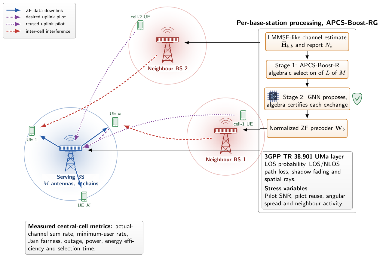
Figure 2.
Architecture of the physics-derived heterogeneous graph network. The engineered features of Table 3 are embedded, exchanged over two message-passing rounds according to Equation (33) and Equation (34) with the bipartite weights and the coherence coupling , pooled into a user context and read out by the two heads of Equation (35). The seed head is an auxiliary output used only in the seed-based ablations. In the principal method, stage one remains identical to APCS-Boost-R and the group-centred exchange head enters selection only through the hybrid key under the certification rule.
Figure 2.
Architecture of the physics-derived heterogeneous graph network. The engineered features of Table 3 are embedded, exchanged over two message-passing rounds according to Equation (33) and Equation (34) with the bipartite weights and the coherence coupling , pooled into a user context and read out by the two heads of Equation (35). The seed head is an auxiliary output used only in the seed-based ablations. In the principal method, stage one remains identical to APCS-Boost-R and the group-centred exchange head enters selection only through the hybrid key under the certification rule.
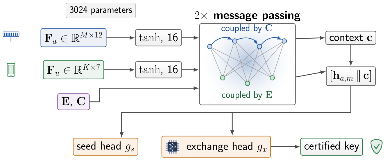
Figure 3.
Joint-stress sum spectral efficiency over the 200 paired realizations for the selected-array methods. Full-array ZF is retained in Table 5 as a different-power reference and is omitted here so that the differences among the selection methods remain visible.
Figure 3.
Joint-stress sum spectral efficiency over the 200 paired realizations for the selected-array methods. Full-array ZF is retained in Table 5 as a different-power reference and is omitted here so that the differences among the selection methods remain visible.
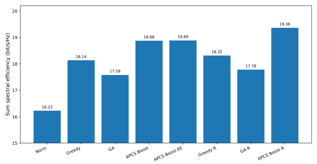
Figure 4.
Paired sum spectral efficiency gains obtained when calibrated information is introduced into norm-initialized greedy search, the fixed-budget genetic algorithm and APCS-Boost. Markers show the mean paired gains and error bars show the corresponding 95% confidence intervals. The largest gain is obtained when the same information is also used by the whitened D-optimal seed.
Figure 4.
Paired sum spectral efficiency gains obtained when calibrated information is introduced into norm-initialized greedy search, the fixed-budget genetic algorithm and APCS-Boost. Markers show the mean paired gains and error bars show the corresponding 95% confidence intervals. The largest gain is obtained when the same information is also used by the whitened D-optimal seed.
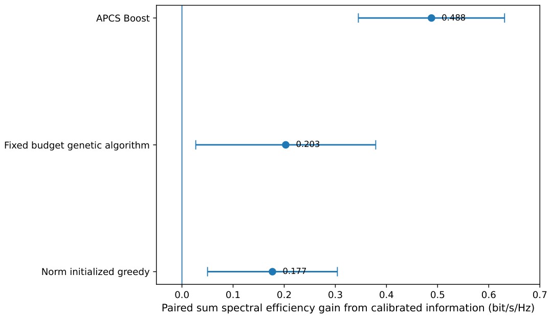
Figure 5.
Paired changes in central-cell sum spectral efficiency relative to APCS-Boost-R for the learned-stage variants over the same evaluation set. Markers show the mean paired changes and error bars show 95% confidence intervals. A symmetric logarithmic horizontal scale with a linear threshold of 0.05 bit/s/Hz is used so that the direct-selection loss and the smaller certified-stage changes can be displayed together. Exact surrogate ranking within the same neighbourhood is included as an attribution reference.
Figure 5.
Paired changes in central-cell sum spectral efficiency relative to APCS-Boost-R for the learned-stage variants over the same evaluation set. Markers show the mean paired changes and error bars show 95% confidence intervals. A symmetric logarithmic horizontal scale with a linear threshold of 0.05 bit/s/Hz is used so that the direct-selection loss and the smaller certified-stage changes can be displayed together. Exact surrogate ranking within the same neighbourhood is included as an attribution reference.
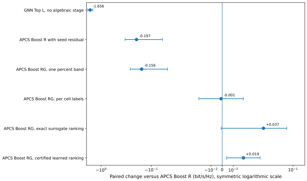
Figure 6.
Controlled single-impairment examinations, each averaged over 100 paired realizations. In every panel the impairments not under study are disabled, so the same user locations, LOS states, shadowing samples and small-scale random variables are reused at every sweep point. Panels (a) and (b) disable neighbour-cell data interference, so the measured report approaches the normalized noise floor while the estimation-error correction in Equation (29) remains dependent on pilot quality and reuse. Panel (c) additionally uses perfect CSI, so spatial correlation is isolated and only normalized receiver noise remains in the report. Panel (d) uses perfect CSI while the neighbour-cell activity factor is varied from zero to one, so only the interference-dependent component of the effective noise varies. Error bars show 95% confidence intervals computed over the 100 pooled paired realizations at each sweep point.
Figure 6.
Controlled single-impairment examinations, each averaged over 100 paired realizations. In every panel the impairments not under study are disabled, so the same user locations, LOS states, shadowing samples and small-scale random variables are reused at every sweep point. Panels (a) and (b) disable neighbour-cell data interference, so the measured report approaches the normalized noise floor while the estimation-error correction in Equation (29) remains dependent on pilot quality and reuse. Panel (c) additionally uses perfect CSI, so spatial correlation is isolated and only normalized receiver noise remains in the report. Panel (d) uses perfect CSI while the neighbour-cell activity factor is varied from zero to one, so only the interference-dependent component of the effective noise varies. Error bars show 95% confidence intervals computed over the 100 pooled paired realizations at each sweep point.
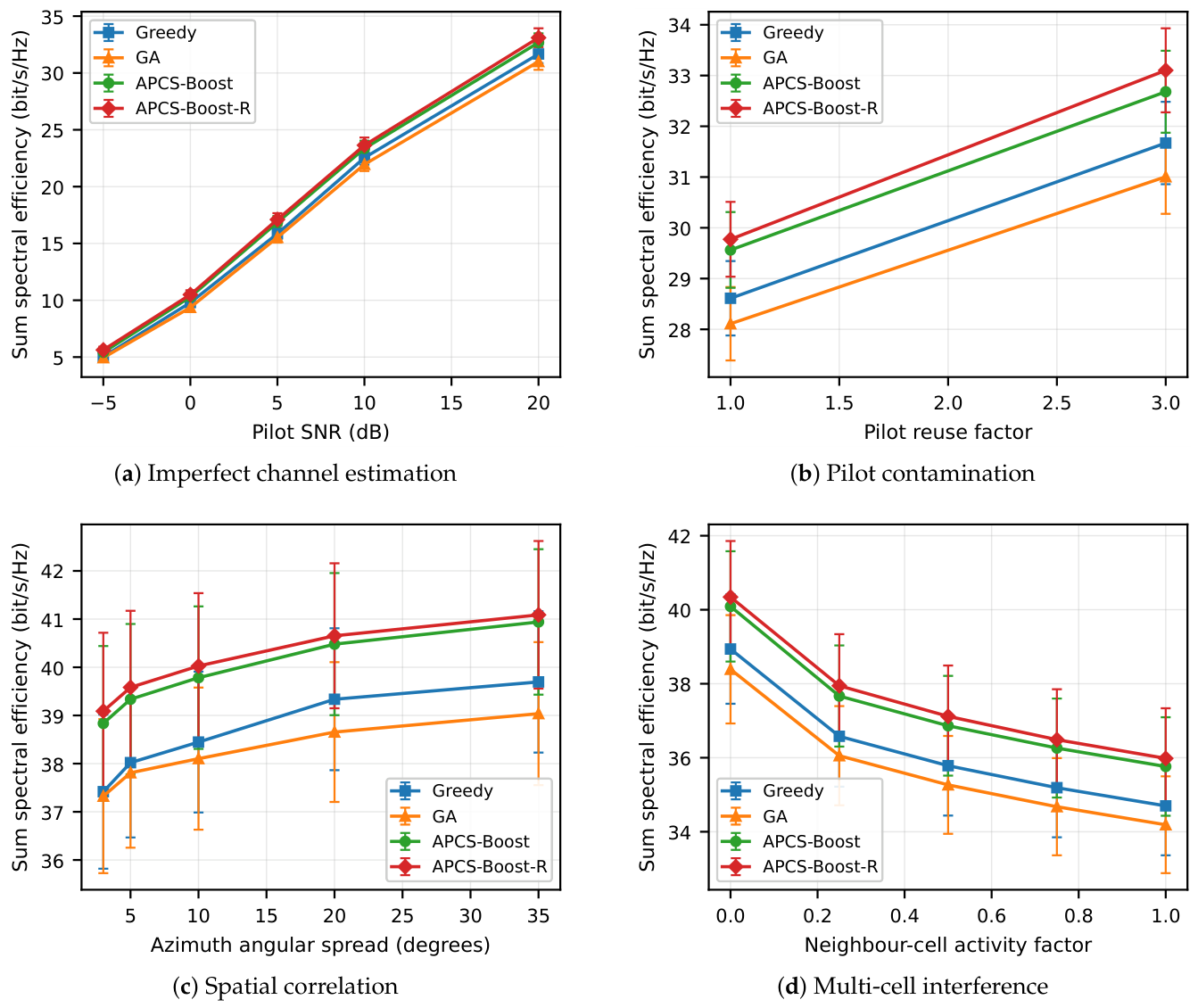
Table 1.
Comparison with Thirteen External State-of-the-Art Antenna-Selection Approach Families. Internal APCS Stages Are Excluded as Independent Comparators.
Table 1.
Comparison with Thirteen External State-of-the-Art Antenna-Selection Approach Families. Internal APCS Stages Are Excluded as Independent Comparators.
| External approach | Reference | Learning | Imperfect CSI | Coupled network | Joint 3GPP stress | Guarantee |
|---|---|---|---|---|---|---|
| Energy-aware ranking and selection | [6,15] | No | No | No | No | None |
| Quasi-distributed genetic search | [7] | No | No | No | No | None |
| Multi-label DNN selector | [9] | Yes | No | No | No | None |
| Deep-learning joint selection and beamforming | [17] | Yes | No | No | No | None |
| ML joint selection and precoding | [18] | Yes | Pilot-based CSI | No | No | None |
| Deep unsupervised selection and beamforming | [19] | Yes | No | No | No | None |
| Fast optimal graph search | [8] | No | No | No | No | Exact for studied size |
| Heuristic joint selection and precoding | [16] | No | No | No | No | None |
| Risk-aware incomplete-CSI selection | [10] | No | Yes | No | No | Risk constraint |
| Learned energy-efficient transmitter configuration | [20] | Yes | Model dependent | No | No | None |
| Boosted learned antenna selection | [21] | Yes | No | No | No | None |
| Certified neural antenna selector | [22] | Yes | Perturbed CSI | No | No | Local robustness certificate |
| Distributed cell-free CNN and GNN design | [11] | Yes | Estimated CSI | Cell-free | No | None |
| Proposed APCS-Boost-R and APCS-Boost-RG framework | This work | Yes | Yes | Three-cell | Yes | Certified stage-one floor |
Table 2.
Definitions of the Three Headroom Figures Used in the Manuscript
| Headroom | Starting subset | Optimized quantity | Interpretation |
|---|---|---|---|
| Approximately 6% | APCS-Boost | Own-cell achieved sum rate | Partial, non-converged diagnostic |
| 21.6% | APCS-Boost-R | Per-cell achieved-rate oracle | Local objective, neighbours fixed |
| 7.2% | APCS-Boost-R | Network partial-response oracle | All-cell rate externality included |
Table 3.
Engineered Node and Coupling Features of the Model
| Feature | Construction |
|---|---|
| Antenna nodes, twelve features | |
| Whitened column energy | log energy under Equation (32), standardized |
| Raw column energy | log energy of the estimate, standardized |
| Aperture block | one-hot membership over four blocks |
| Array position | index scaled to |
| Peak coherence | maximum inter-column correlation, standardized |
| Mean coherence | mean inter-column correlation, standardized |
| User concentration | Herfindahl index of per-user shares, standardized |
| Determinant gain | first-step gain of Equation (19), log, standardized |
| Subset membership | centred flag, zero when unconditioned |
| User nodes, seven features | |
| Interference report | , standardized |
| Error variance | from Equation (31), standardized |
| Effective noise | from Equation (29), standardized |
| Row energy | log user channel energy, standardized |
| Estimation reliability | energy over energy plus , centred |
| Relative report | report over its mean, centred |
| Subset coverage | whitened covered-energy ratio, centred |
| Couplings | |
| Bipartite weights | whitened per-user energy fractions |
| Antenna coupling | normalized squared inter-column correlations |
Table 4.
3GPP-Derived Simulation Parameters
| Parameter | Value |
|---|---|
| Scenario and carrier | UMa, 3.5 GHz |
| Cells and inter-site distance | 3, 500 m |
| Available/active antennas | , |
| Users per cell | |
| BS and user heights | 25 m, 1.5 m |
| User distance range | 35 m to 220 m |
| Spatial rays | 20 |
| Joint pilot SNR and reuse | 10 dB, 1 |
| Joint azimuth angular spread | |
| Joint neighbour activity | 1.0 |
| Data SNR | 10 dB |
| Physical transmit power | 10 W |
| PA efficiency, RF-chain power | 0.40, 0.50 W |
| Baseband power | 5 W |
| Coverage factor , shortlist q | 0.55, 12 |
| Condition-number limit | |
| Refinement rounds, APCS-Boost/APCS-Boost-R | 3/8 |
| APCS-Boost-RG rounds , weight , band , margin | 6, 0.03, 0, |
| APCS-Boost-RG corpus scenes, training, validation | 160, 130, 30 |
| APCS-Boost-RG hidden units, epochs | 16, 400 |
| Replications | 5 |
| Joint/sweep realizations per replication | 40/20 |
Table 5.
Joint 3GPP-Derived Stress Comparison at 10 dB Data SNR over 200 Paired Realizations. External comparator families are cited in the method column and are reimplemented under the same channel realizations, power model and active-chain budget. The full-array row is a reference rather than a selection method. The active-chain column reports the mean active chains and the time column reports selection computation time, which excludes interference-report acquisition and feedback.
Table 5.
Joint 3GPP-Derived Stress Comparison at 10 dB Data SNR over 200 Paired Realizations. External comparator families are cited in the method column and are reimplemented under the same channel realizations, power model and active-chain budget. The full-array row is a reference rather than a selection method. The active-chain column reports the mean active chains and the time column reports selection computation time, which excludes interference-report acquisition and feedback.
| Method | Sum SE | Min. rate | Jain | Outage | Active | Power | EE | Time |
|---|---|---|---|---|---|---|---|---|
| (bit/s/Hz) | (bit/s/Hz) | fraction | chains | (W) | (bit/J/Hz) | (ms) | ||
| Norm ranking [15] | 16.226 | 0.115 | 0.603 | 0.366 | 16.00 | 38.00 | 0.427 | 0.504 |
| Norm-initialized greedy [6] | 18.137 | 0.202 | 0.658 | 0.314 | 16.00 | 38.00 | 0.477 | 57.775 |
| Genetic search [7] | 17.578 | 0.179 | 0.666 | 0.306 | 16.00 | 38.00 | 0.463 | 41.302 |
| APCS-Boost | 18.876 | 0.221 | 0.675 | 0.294 | 16.00 | 38.00 | 0.497 | 12.728 |
| APCS-Boost-EE | 18.885 | 0.221 | 0.675 | 0.291 | 15.98 | 37.99 | 0.497 | 21.251 |
| Greedy-R | 18.315 | 0.175 | 0.654 | 0.316 | 16.00 | 38.00 | 0.482 | 75.431 |
| GA-R | 17.781 | 0.164 | 0.651 | 0.305 | 16.00 | 38.00 | 0.468 | 48.494 |
| APCS-Boost-R | 19.364 | 0.208 | 0.678 | 0.286 | 16.00 | 38.00 | 0.510 | 20.376 |
| Full-array ZF [2] | 28.702 | 0.435 | 0.723 | 0.211 | 64.00 | 62.00 | 0.463 | n/a |
Table 6.
Learned-Ranking Ablation Over the Same 200 Paired Realizations. Bold marks the best column value by point estimate. Exact surrogate ranking evaluates every feasible single-exchange candidate within the current neighbourhood. The time column reports environment-normalized selection computation time after cross-environment calibration with the APCS-Boost-R runtime.
Table 6.
Learned-Ranking Ablation Over the Same 200 Paired Realizations. Bold marks the best column value by point estimate. Exact surrogate ranking evaluates every feasible single-exchange candidate within the current neighbourhood. The time column reports environment-normalized selection computation time after cross-environment calibration with the APCS-Boost-R runtime.
| Method | Sum SE | SE versus APCS-Boost-R | Time |
|---|---|---|---|
| (bit/s/Hz) | (bit/s/Hz) | (ms) | |
| GNN-Top-L | 17.707 | 4.4 | |
| APCS-Boost-R with seed residual | 19.167 | 24.8 | |
| APCS-Boost-RG, | 19.207 | 30.0 | |
| APCS-Boost-RG, per-cell labels | 19.363 | 23.4 | |
| APCS-Boost-R | 19.364 | reference | 20.4 |
| APCS-Boost-RG, exact surrogate ranking | 19.401 | 23.4 | |
| APCS-Boost-RG | 19.383 | 24.0 |
Disclaimer/Publisher’s Note: The statements, opinions and data contained in all publications are solely those of the individual author(s) and contributor(s) and not of MDPI and/or the editor(s). MDPI and/or the editor(s) disclaim responsibility for any injury to people or property resulting from any ideas, methods, instructions or products referred to in the content. |
© 2026 by the authors. Licensee MDPI, Basel, Switzerland. This article is an open access article distributed under the terms and conditions of the Creative Commons Attribution (CC BY) license (http://creativecommons.org/licenses/by/4.0/).
Copyright: This open access article is published under a Creative Commons CC BY 4.0 license, which permit the free download, distribution, and reuse, provided that the author and preprint are cited in any reuse.