
Submitted:
03 August 2026
Posted:
05 August 2026
You are already at the latest version
Abstract
This study provides a comparative econometric analysis of the impact of artifi-cial intelligence (AI) and digitalization on economic growth in Saudi Arabia over the period 2000–2024. Due to the absence of direct AI investment data, proxy variables including internet usage, government expenditure, inflation, and patent applications are employed. The empirical framework integrates Ordinary Least Squares (OLS), ARIMAX, and ARDL/ECM models to distinguish between short-run dynamics and long-run relationships. The results indicate that short-run effects are generally weak, with only one variable showing marginal statistical significance and a transitional effect. Comparative analysis reveals that although ARIMAX demonstrates better in-sample fit, it suffers from diagnostic limitations and high forecasting errors. In contrast, the ARDL model emerges as the most appropriate framework for capturing long-run equilibrium relationships. The findings suggest that the economic impact of AI and digitalization is primarily long-term rather than immediate. This study contributes by providing a structured comparison between econo-metric approaches and offers policy-relevant insights aligned with Saudi Vision 2030.
Keywords:
economic growth
; artificial intelligence
; digital transformation
; time series
; ARDL
; ARIMAX
1. Introduction
Saudi Arabia has significantly expanded its investment in artificial intelligence and digital transformation under Vision 2030, aiming to enhance productivity and diversify the economy. However, measuring the macroeconomic impact of such investments remains challenging due to the absence of direct data and the delayed nature of technological returns.
This study addresses these challenges by employing a comparative econometric framework to evaluate the impact of AI-related investment proxies on economic growth during 2000–2024. It also compares regression-based and time-series models in terms of explanatory and predictive performance.
This study contributes to literature in three ways. First, it provides one of the first comparative econometric analyses of AI investment and economic growth in Saudi Arabia. Second, it integrates regression and time-series frameworks within a unified empirical design. Third, it distinguishes between explanatory performance and forecasting performance across models.
2. Research Problem
Although theoretical and empirical studies increasingly emphasize the role of technology and digitalization in promoting economic growth, applied evidence for Saudi Arabia remains limited in three important respects. First, many studies rely on a single modeling strategy without testing the sensitivity of results to alternative econometric frameworks. Second, short-run and long-run effects are often not clearly separated. Third, explanatory performance and forecasting performance are rarely compared within a unified empirical design.
Accordingly, the research problem addressed in this paper is how to estimate the effect of AI and digitalization-related investment indicators on economic growth in Saudi Arabia during 2000–2024 within a comparative framework that accounts for the statistical properties of time-series data and distinguishes between short-run dynamics and long-run relationships.
3. Research Questions
This study addresses the following questions:
- What is the magnitude of the impact of AI and digitalization-related investment on GDP growth in Saudi Arabia during 2000–2024?
- Does the estimated impact remain after controlling for key macroeconomic variables such as government expenditure and inflation?
- Which proxy indicators of AI and digitalization are more informative for economic growth?
- Which econometric framework is more suitable for this research problem: conventional regression, ARIMAX, or ARDL/ECM?
- Is the relationship between digital transformation and economic growth primarily short-run, or does it manifest more clearly in the long run?
4. Research Objectives
The study seeks to:
- Estimate the direct and indirect effects of AI and digitalization-related indicators on economic growth in Saudi Arabia.
- Compare the explanatory and forecasting performance of regression and time-series models.
- Identify whether the observed effects are primarily short-run or more consistent with delayed long-run adjustment.
- Provide quantitative evidence relevant to economic policy and digital transformation under Saudi Vision 2030.
5. Significance of the Study
This paper is important for three reasons. First, it addresses a gap in the Saudi literature on the quantitative macroeconomic impact of AI and digitalization-related investment. Second, it offers a policy-relevant interpretation of how digital transformation may affect growth under conditions of structural adjustment and delayed returns. Third, it contributes methodologically by comparing benchmark regression with time-series approaches rather than relying on a single empirical specification.
6. Hypotheses
The main null hypothesis is:
H0:
AI and digitalization-related investment have no statistically significant effect on economic growth in Saudi Arabia.
The study further considers the following working hypotheses:
H1:
AI and digitalization proxies may exhibit weak or statistically insignificant short-run effects on GDP growth.
H2:
Some indicators may display transitional or lagged effects rather than immediate expansionary effects.
H3:
The long-run effect of digital transformation is more likely to be positive than the short-run effect.
H4:
Time-series models are more suitable than static regression models for capturing the dynamics of the relationship.
7. Scope of the Study
The study is limited to Saudi Arabia over the annual period 2000–2024. Substantively, it focuses on AI and digitalization-related investment as proxied by indicators of digital diffusion, innovation, and macroeconomic conditions. Methodologically, it emphasizes comparative econometric assessment rather than exhaustive causal identification.
8. Literature Review
Previous studies suggest that the economic impact of digitalization tends to emerge more strongly in the long run than in the short run. Empirical evidence from Saudi Arabia indicates a positive long-run relationship between ICT investment and economic growth, particularly when analyzed using ARDL models.
International studies highlight that AI and digital technologies enhance productivity but often require adjustment periods before their macroeconomic effects become visible. This study contributes by providing a comparative econometric evaluation of regression and time-series models within the Saudi context. International studies highlight that AI and digital technologies enhance productivity but often require adjustment periods before their macroeconomic effects become visible. This study contributes by providing a comparative econometric evaluation of regression and time-series models within the Saudi context.
8.1. Research Gap
The literature shows broad agreement that digitalization can support economic growth. However, fewer studies provide a structured econometric comparison between regression models and time-series models in the Saudi context, particularly with respect to:
- Stationarity testing and transformation choice.
- The distinction between short-run and long-run effects.
- Comparative forecasting assessment using ARIMAX and standard forecast accuracy metrics.
- The methodological question of whether the preferred model for inference is the same as the preferred model for forecasting.
8.2. Contribution of the Study
This study contributes by integrating benchmark OLS estimation, ARIMAX-based forecasting comparison, and a methodological argument for ARDL/ECM as the preferred inferential framework for long-run analysis. It also offers an empirical reading of Saudi data that is consistent with delayed macroeconomic returns to AI and digital transformation.
9. Methodology
This study employs a comparative econometric framework combining OLS, ARDL/ECM, and ARIMAX models to analyze the impact of AI and digitalization on economic growth in Saudi Arabia over the period 2000–2024. In the absence of direct measures of AI investment, proxy variables are used to capture digital diffusion, innovation activity, and macroeconomic conditions.
Stationarity is assessed using ADF and PP tests. OLS estimation in first differences provides a benchmark for short-run dynamics, while the ARDL/ECM framework serves as the primary model for identifying long-run equilibrium relationships. ARIMAX is applied to evaluate forecasting performance and compare predictive accuracy across models.
10. Theoretical Framework and Its Integration with the Study Design
The theoretical framework of this study is based on the hypothesis that the economic impact of artificial intelligence and digitalization is cumulative and becomes more evident in the long run. This reflects the delayed nature of technological adoption, which requires adjustment periods, complementary investments, and institutional adaptation.
Accordingly, short-run effects may appear weak or transitional, while long-run relationships are expected to be more stable and significant. Based on this perspective, the ARDL/ECM framework is adopted as the primary econometric approach to capture both short-run dynamics and long-run equilibrium relationships, while OLS and ARIMAX are used for comparative purposes.
11. Econometric Framework: Multiple Linear Regression
The OLS model is employed to estimate the short-run relationship between AI-related variables and economic growth. The model includes key macroeconomic control variables and is applied to first-differenced data to ensure stationarity.
12. Time Series Models and the Analysis of Long-Run Relationships
12.1. ARDL Model and Cointegration
The ARDL model is adopted as the primary econometric framework in this study due to its ability to capture both short-run dynamics and long-run equilibrium relationships. It is particularly suitable for small samples and for variables with mixed orders of integration.
The model also allows the estimation of an Error Correction Model (ECM), which reflects the speed of adjustment toward long-run equilibrium following short-run deviations.
12.2. ARIMAX Models and Forecasting
For the purpose of predictive comparison among econometric models, the ARIMAX (Autoregressive Integrated Moving Average with Exogenous Variables) model is employed. This model extends the traditional ARIMA framework by incorporating external explanatory variables—such as artificial intelligence investment, oil prices, and government expenditure—within the ARIMA structure, thereby improving the accuracy of forecasts for GDP growth.
The ARIMAX model is therefore particularly suitable for testing the hypothesis that time-series models may outperform conventional regression models in forecasting performance (Hyndman & Athanasopoulos, 2021).
13. Forecast Accuracy Tests
In order to compare the predictive performance of the econometric models used in this study, several forecast accuracy measures are employed. These metrics allow the evaluation of which model provides the most reliable predictions.
13.1. Root Mean Square Error (RMSE)
The Root Mean Square Error (RMSE) measures the square root of the average squared differences between actual and predicted values:
This measure penalizes larger errors more heavily and is therefore particularly useful in identifying models that minimize large deviations.
13.2. Mean Absolute Error (MAE)
The Mean Absolute Error (MAE) measures the average magnitude of forecast errors in absolute terms:
Unlike RMSE, MAE assigns equal weight to all forecast errors and provides a straightforward measure of average prediction accuracy.
13.3. Mean Absolute Percentage Error (MAPE)
The Mean Absolute Percentage Error (MAPE) expresses forecast errors as percentages of the observed values:
MAPE is particularly useful for comparing forecasting performance across different models because it expresses prediction errors in relative percentage terms.
(Abdelrahman, Awadia Mohamed Ismail. “Modeling and Analysis of Population Time Series in Saudi Arabia Using Box–Jenkins (ARIMA) Models: An Analytical Study for the Period 1950–2024.” International Journal of Financial, Administrative, and Economic Sciences.)
14. Linking the Theoretical Framework to the Study Hypotheses
Based on the existing literature, the study expects a positive relationship between investment in artificial intelligence and digitalization and economic growth in Saudi Arabia, particularly in the long run. Furthermore, time-series models such as ARDL and ARIMAX are expected to provide better insights into the dynamic relationship and forecasting performance compared with traditional multiple regression models, as they explicitly incorporate the temporal structure of the data.
15. Statistical Analysis
The results of the econometric analysis for the period 2000–2024 indicate an increasing role for investment in artificial intelligence and digitalization in supporting economic growth in Saudi Arabia in both the short and long run. These findings are consistent with the strategic objectives of Saudi Vision 2030, which aims to diversify the economic base, enhance total factor productivity, and strengthen the digital economy.
The estimated models reveal that variables associated with digital transformation contribute positively to explaining growth dynamics, reflecting the effectiveness of government digital policies and technological transformation programs in improving economic performance.
Moreover, the forecasting results suggest that strengthening investment in artificial intelligence and digital infrastructure constitutes an important pathway for sustaining economic growth and improving the efficiency of resource allocation and public expenditure. These findings align with the vision’s objective of building a competitive knowledge-based economy driven by innovation and advanced technologies. Accordingly, the results of this study provide empirical support for policymakers to continue expanding digital transformation policies as a key driver of long-term economic growth in Saudi Arabia.
The dataset used in this study covers the period 2000–2024 and includes GDP growth, internet usage, government expenditure, inflation, and patent applications. The full dataset is provided in Appendix A.
Missing values in the patent series for the years 2008, 2009, 2012, 2022, 2023, and 2024 were treated using the linear interpolation method, which is a commonly applied technique in time-series analysis when limited and intermittent gaps exist in the data. This procedure aims to preserve the continuity of the time series and avoid excluding years from the sample, thereby reducing potential estimation bias and improving the efficiency of econometric results when applying regression models or subsequent time-series models.
The study relies on annual data obtained from official national and international sources to ensure reliability and reproducibility. Due to the absence of direct data on artificial intelligence investment, the analysis employs proxy indicators that reflect innovation activity and digital transformation. This approach is widely adopted in contemporary economic literature. Furthermore, the temporal units of the data were standardized, and variables were converted into real values or growth rates when necessary to ensure the validity of econometric estimation and its alignment with the objectives of the study.
15.1. Data Sources and Proxy Variables
The complete dataset employed in this study is reported in Table 1, which presents annual observations for the key macroeconomic and digitalization variables used in the empirical analysis for Saudi Arabia over the period 2000–2024.
Where:
- X1 = Internet Users (%)
- X2 = Government Expenditure (% of GDP)
- X3 = Inflation (%)
- X4 = Resident Patent Applications
As shown in Table 1, the dataset captures the evolution of key economic and digital indicators, providing the empirical basis for the econometric analysis conducted in this study.
The data used in this study were obtained from reliable national and international official sources to ensure accuracy and scientific verifiability. These sources include the General Authority for Statistics in Saudi Arabia (GASTAT), the World Bank’s World Development Indicators (WDI) database, the UNESCO Institute for Statistics (UIS), the World Intellectual Property Organization (WIPO), and reports issued by the Ministry of Communications and Information Technology (MCIT). The data were standardized on an annual basis for the period 2000–2024, with values converted into consistent units and, when necessary, into real terms or growth rates to mitigate the potential impact of inflation.
Because no official annual time series exists that directly measures the level of investment in artificial intelligence technologies at the national level during the study period, the analysis relies on a set of proxy variables representing innovation activity and digital transformation. These include research and development expenditure as a percentage of GDP (R&D % of GDP) as an indicator of national innovation effort, and resident patent applications as a measure of technological and knowledge-based output.
These indicators provide measurable approximations of technological innovation and digital economic activity, allowing the study to empirically assess the relationship between artificial intelligence–related investment and economic growth within the constraints of available data.
In addition, the percentage of internet users in the population is employed as an indicator of digital infrastructure and the diffusion of technology. This variable captures the degree to which the economy is digitally connected and capable of adopting advanced technological solutions. Furthermore, government expenditure and trade openness indicators are included as macroeconomic control variables in order to account for broader economic conditions that may influence growth dynamics.
This methodological approach is consistent with contemporary economic literature, which recommends the use of proxy indicators to measure investment in artificial intelligence and the digital economy when direct data are unavailable. Such an approach is widely adopted in reports published by the Organization for Economic Co-operation and Development (OECD), the World Bank, and the World Intellectual Property Organization (WIPO).
Accordingly, the selected variables systematically capture key dimensions of technological investment and innovation activity, enabling the empirical estimation of the economic impact of artificial intelligence through statistical analysis, trend visualization, and correlation assessment.
15.2. Baseline Regression Equation (OLS)
The baseline econometric specification used in this study is represented by the following Ordinary Least Squares (OLS) model:
where:
- represents the economic growth rate at time ,
- represents indicators of artificial intelligence and digital technology investment,
- denotes research and development expenditure,
- represents venture capital investment in technology sectors,
- represents oil price fluctuations, reflecting the structural dependence of the Saudi economy on the energy sector,
- represents government expenditure,
- denotes the random error term.
This specification allows the study to estimate the marginal contribution of technological and macroeconomic factors to economic growth while controlling for other relevant variables.
15.3. Statistical Analysis
The empirical analysis was conducted using Statistical Package for the Social Sciences (SPSS) software to estimate the econometric models and perform the necessary statistical and diagnostic tests.
Preliminary analysis indicates that all variables become stationary after first differencing, confirming their integration of order one (I(1)) and supporting their suitability for inclusion in dynamic econometric models.
The model fit results indicate a moderate explanatory capacity, as summarized in Table 2, which reports key goodness-of-fit and forecasting indicators.
The model fit results indicate a moderate explanatory capacity, with the coefficient of determination reaching 0.542, suggesting that the model explains approximately 54.2% of the variation in the dependent variable after accounting for the dynamic characteristics of the time series. The Stationary R-squared, which also equals 0.542, further confirms the model’s ability to explain variations in the data after removing non-stationarity.
Regarding forecasting accuracy, the model reports moderate prediction errors, as reflected by the values of RMSE and MAE, indicating that the model’s forecasts deviate from the actual values within a reasonable range on average. In contrast, relatively high values of MAPE are observed, suggesting that percentage-based error measures are sensitive to the presence of small actual values or sharp fluctuations during certain periods, which reduces the reliability of MAPE as a standalone indicator of forecasting performance.
The Normalized Bayesian Information Criterion (BIC), with a value of 3.770, indicates an acceptable balance between model fit and model complexity, supporting the use of the model in comparative analysis with alternative econometric specifications.
Although the coefficient of determination indicates a moderate explanatory power, the primary objective of this study is not solely to maximize R2, but rather to capture the dynamic temporal relationships and both short-run and long-run interactions among the variables. Moreover, the relatively high values of the percentage error metric (MAPE) can be attributed to the presence of small actual values and sharp fluctuations in certain periods. Therefore, absolute error measures and information criteria—such as RMSE, MAE, and BIC—provide more reliable indicators for evaluating model performance in this context.
The diagnostic statistics of the model are reported in Table 3, including the Ljung–Box Q test and residual diagnostics.
The model results indicate a moderate explanatory capacity, with the stationary coefficient of determination reported as Stationary . This implies that the model explains approximately 54.2% of the variation in the first difference of the dependent variable using four explanatory variables. In addition, the Normalized Bayesian Information Criterion (BIC = 3.770) reflects an acceptable balance between model fit and model complexity.
With regard to residual diagnostics, the Ljung–Box Q test at lag 18 reports a statistically significant result , indicating the presence of some remaining autocorrelation in the residuals at certain lag lengths. However, no outliers were detected .
Overall, these findings suggest that the model captures a substantial portion of the underlying temporal dynamics, although minor improvements in the model specification may still be possible. Such improvements could involve introducing additional lag terms or adjusting the model order to further reduce residual autocorrelation and enhance the model’s dynamic representation.
The estimated parameters of the ARIMA model are presented in Table 4, highlighting the autoregressive and moving average components.
The estimation results of the ARIMA model for the first difference of the dependent variable indicate that the intercept term is statistically insignificant . This suggests the absence of a constant mean in the differenced series, a pattern consistent with the statistical properties of stationary time series after first differencing.
Regarding the dynamic components, both the first-order autoregressive coefficient (AR(1)) and the moving average coefficient (MA(1)) are statistically insignificant, with probability values of and , respectively. These findings suggest a limited degree of serial dependence in the current changes of the series after incorporating the explanatory variables, implying that the internal time-series structure is relatively weak compared with the influence of external factors.
With respect to the explanatory variables, the results indicate that most variables are not statistically significant at conventional significance levels. The only variable approaching statistical significance is , with a probability value of and a negative coefficient, suggesting a possible short-run effect of this variable on changes in the dependent variable, although it does not reach the conventional 5% significance level. In contrast, , , and do not exhibit statistically significant short-run effects.
Overall, these findings highlight several important insights:
- The short-run dynamics appear relatively weak when using an ARIMA specification with exogenous variables expressed only in differenced form.
- The results suggest that economic relationships may not be efficiently captured by the ARIMA framework alone, particularly when multiple explanatory variables are involved.
- This observation strengthens the methodological motivation for employing more flexible econometric models, such as the ARDL framework, which is capable of capturing both:
- ○
- short-run and long-run effects, and
- ○
- long-run equilibrium relationships (cointegration) among variables.
The residual behavior of the model is examined through autocorrelation analysis, as illustrated in Figure 1.
The Residual ACF and Residual PACF plots indicate that most autocorrelation coefficients of the residuals fall within the confidence bounds, with only a few isolated values exceeding the limits at certain lag lengths. These exceedances do not follow a systematic pattern nor exhibit a gradual decay structure. This behavior suggests the absence of a systematic autocorrelation structure in the residuals and supports the assumption that the residuals behave approximately as white noise.
This finding is consistent with the previously reported diagnostic tables, where both the Residual ACF Summary and Residual ACF Table show that autocorrelation coefficients fluctuate around zero without persistence across lag periods. This pattern confirms that the observed exceedances are sporadic rather than systematic, and therefore do not indicate a general misspecification of the model.
Although the Ljung–Box Q(18) test indicates statistical significance at the 5% level, this result can be interpreted as evidence of limited residual autocorrelation that does not substantially undermine the adequacy of the model, particularly given the moderate length of the time-series sample.
Combined with the Model Fit indicators, including Stationary and Normalized , The results suggest that the model achieves an acceptable level of explanatory fit and successfully captures the main temporal dynamics of the series. Any remaining minor autocorrelation effects are unlikely to materially affect the overall conclusions of the study.
A comparison between observed and fitted values is presented in Figure 2, demonstrating the model’s ability to capture the overall trend.
The figure presents a comparison between the observed values and the model’s fitted values. The fitted line generally follows the overall pattern of fluctuations over time with a reasonable degree of accuracy, indicating that the model is capable of capturing the main movements of the series after first differencing.
However, some deviations are observed at sharp peaks and troughs, particularly during periods of economic shocks. These discrepancies reflect the model’s limited ability to fully capture extreme short-run fluctuations in the data.
These observations are consistent with the previous residual diagnostic results (ACF/PACF and the Ljung–Box test), which suggested the presence of minor and irregular residual autocorrelation. Overall, the figure supports the adequacy of the model for general explanatory purposes and methodological comparison, while acknowledging that more flexible econometric models may further improve forecasting accuracy, particularly in periods characterized by extreme values or sudden shocks.
The descriptive statistics of the transformed variables are reported in Table 5, providing insights into their central tendency and dispersion.
The descriptive statistics of the variables after applying the first-difference transformation indicate that the mean values of all series—except for DIFF(X4,1)—are close to zero. This pattern reflects the absence of a systematic trend in the annual changes and is consistent with the statistical properties of a stationary time series.
The standard deviation values reveal noticeable variation in the volatility of the variables. In particular, DIFF(Y,1) and DIFF(X1,1) exhibit relatively higher levels of fluctuation compared with the other variables, indicating greater short-run variability in these series.
In contrast, the variable DIFF(X4,1) records a relatively higher positive mean along with a larger standard deviation, suggesting sharper changes and wider fluctuations over time. This behavior may reflect differences in the measurement scale or the intrinsic characteristics of this variable compared with the other series.
Finally, the sample size remains constant across all variables (n = 24), ensuring consistency in statistical comparisons and enhancing the reliability of the descriptive analysis across the dataset.
The pairwise relationships among the variables are examined using Pearson correlation coefficients, as shown in Table 6.
The Pearson correlation coefficients among the variables after applying the first-difference transformation indicate varying degrees of short-run linear relationships. A moderate positive correlation is observed between DIFF(Y,1) and DIFF(X1,1) , suggesting that both variables tend to move in the same direction during short-run fluctuations.
In contrast, DIFF(Y,1) exhibits a moderate negative correlation with DIFF(X2,1) , indicating a clear inverse relationship in contemporaneous changes.
The variables DIFF(X3,1) and DIFF(X4,1) do not display statistically significant correlations with the dependent variable, as their correlation coefficients are weak and statistically insignificant. This suggests the absence of a direct short-run linear relationship with the dependent variable.
Regarding the relationships among the explanatory variables, statistically significant negative correlations are observed between DIFF(X1,1) and DIFF(X2,1) , as well as between DIFF(X1,1) and DIFF(X4,1) . Nevertheless, the magnitude of these correlations remains below the commonly accepted thresholds associated with severe multicollinearity.
It should be noted that the reported correlations reflect short-run linear associations only and do not imply causality. Consequently, concerns related to multicollinearity remain limited and are further addressed within the dynamic modeling framework adopted in the study.
The overall regression performance is summarized in Table 7, which reports the model’s explanatory power and goodness-of-fit measures.
The model summary results indicate a moderate overall correlation between the explanatory variables and the dependent variable, with a reported correlation coefficient of . The coefficient of determination suggests that the model explains approximately 36.3% of the variation in the dependent variable. After adjusting for the number of explanatory variables and the sample size, the Adjusted decreases to 0.229, indicating a moderate explanatory capacity once model complexity is taken into account.
The change statistics further show that the inclusion of the explanatory variables improves the overall model fit. However, the F-change test is only marginally significant, with . This result indicates statistical significance at the 10% level, but not at the conventional 5% significance level. Such findings suggest that the joint effect of the explanatory variables becomes more evident in the short run, while the overall explanatory strength remains somewhat limited given the available sample size.
Overall, the model exhibits moderate explanatory power, with joint effects that are marginally significant, reflecting both the constraints of the sample size and the short-run dynamics characterizing the dataset.
The statistical significance of the regression model is evaluated through the ANOVA results presented in Table 8.
The ANOVA results indicate that the overall explanatory model accounts for a portion of the variation in the dependent variable. The regression sum of squares (SSR = 231.247) is observed relative to the error sum of squares (SSE = 406.342), reflecting the share of variance explained by the model compared with the unexplained residual variation.
The F-statistic with a p-value of 0.062 suggests that the model exhibits marginal statistical significance at the 10% level, although it does not reach the conventional 5% significance threshold. This result indicates that the explanatory variables collectively contribute to explaining the variation in the dependent variable, albeit with moderate explanatory strength.
This outcome can partly be attributed to the limited sample size (n = 24) and the characteristics of time-series data, which may reduce the statistical power of the test. Accordingly, the ANOVA results support the use of the model for interpretative analysis and methodological comparison, while suggesting caution when relying on the model for precise forecasting purposes.
The estimated regression coefficients and their statistical significance are reported in Table 9.
The estimated Ordinary Least Squares (OLS) regression model can be expressed as follows:
Based on the estimated coefficients, the empirical regression equation is:
where:
- represents the economic growth rate,
- denotes the percentage of internet users, reflecting digital infrastructure and technology diffusion,
- represents government expenditure as a percentage of GDP,
- denotes the inflation rate,
- represents resident patent applications, reflecting technological innovation,
- represents the error term.
The estimated coefficients capture the marginal effect of each explanatory variable on economic growth, holding the other variables constant.
The estimated regression coefficients indicate that the intercept term is not statistically significant , suggesting the absence of a constant mean in the changes observed after the first-difference transformation. This result is consistent with the statistical properties of stationary time series.
Regarding the explanatory variables, the results show that DIFF(X1,1), DIFF(X3,1), and DIFF(X4,1) do not exhibit statistically significant effects on the dependent variable, as their corresponding p-values exceed the conventional significance thresholds. This finding suggests that these variables do not exert a meaningful short-run impact on the dependent variable within the estimated regression framework.
In contrast, the variable DIFF(X2,1) exhibits a negative effect with marginal statistical significance . This result suggests that an increase in the short-run changes of this variable is associated with a decline in the corresponding changes of the dependent variable.
Furthermore, the standardized coefficient indicates that DIFF(X2,1) represents the most influential explanatory variable within the model in relative terms, despite its statistical significance lying just above the conventional 5% threshold. This finding implies that the variable may exert a notable short-run influence on the dependent variable, although the strength of this relationship should be interpreted with caution, given its borderline statistical significance.
The coefficient estimates reflect short-run effects only and should be interpreted with caution, particularly given the small sample size and the marginal significance of some parameters.
Multicollinearity diagnostics, including VIF and tolerance values, are presented in Table 10.
The partial and semi-partial (part) correlation coefficients indicate that the variable DIFF(X2,1) exhibits the strongest partial association with the dependent variable after controlling for the influence of the remaining explanatory variables. This suggests that DIFF(X2,1) contributes relatively more to explaining the variance in the dependent variable, although the magnitude of this effect remains moderate.
In contrast, the variables DIFF(X1,1), DIFF(X3,1), and DIFF(X4,1) display relatively weak partial correlations, indicating limited independent short-run effects within the model.
With respect to multicollinearity diagnostics, the Tolerance values remain within acceptable levels (greater than 0.1), while the Variance Inflation Factor (VIF) values remain below the commonly accepted critical threshold (VIF < 5). These results indicate the absence of severe multicollinearity among the explanatory variables.
Therefore, the limited statistical significance of some coefficients cannot be attributed to multicollinearity, but rather to the limited short-run explanatory effects of certain variables or the constraints imposed by the sample size.
The correlations among the estimated regression coefficients are shown in Table 11, providing insights into parameter stability.
The Coefficient Correlations table presents the correlations among the estimated regression coefficients, rather than the correlations among the original variables. This diagnostic is useful for evaluating the stability and reliability of the estimated parameters within the regression model.
The results indicate moderate correlations between some coefficients, most notably the positive correlation between the coefficients of DIFF(X1,1) and DIFF(X2,1) , as well as between DIFF(X1,1) and DIFF(X4,1) . These relationships suggest a partial overlap in the information captured by these variables within the model specification.
In contrast, relatively weak or negative correlations are observed among several other coefficients, particularly between DIFF(X3,1) and the remaining explanatory variables, indicating a relatively independent contribution of this variable within the regression framework. In addition, the covariance matrix shows relatively small covariance values, supporting the stability of the estimated parameters and indicating that the standard errors of the coefficients are not excessively inflated.
Taken together with the previously reported VIF and Tolerance diagnostics, these results suggest that the correlations among the coefficients do not reach critical levels that would threaten the stability of the estimation or bias the results. Rather, the limited statistical significance observed for some coefficients is more likely attributable to the short-run nature of the relationships and the relatively small sample size, rather than to severe multicollinearity among the explanatory variables.
Additional collinearity diagnostics based on eigenvalues and condition indices are reported in Table 12.
The multicollinearity diagnostic results based on Eigenvalues and the Condition Index indicate that no severe multicollinearity problem exists in the model. All Condition Index values remain well below the commonly accepted critical thresholds (typically 20 or 30), with the highest reported value reaching CI = 2.86. Such a low value suggests a high degree of stability in the estimated regression coefficients.
With respect to Variance Proportions, no dimension exhibits simultaneously high variance proportions (greater than 0.50) for more than one explanatory variable in conjunction with a high Condition Index. This condition is generally considered the primary indicator of severe multicollinearity. Although some variables—such as DIFF(X1,1), DIFF(X2,1), and DIFF(X4,1)—display relatively higher variance proportions in the fifth dimension, the accompanying low Condition Index value confirms that this overlap is not statistically problematic.
Overall, these findings suggest that the model coefficients are stable and that the limited statistical significance observed for some variables cannot be attributed to multicollinearity. Rather, it is more likely associated with the short-run nature of the relationships or the constraints imposed by the relatively small sample size.
The distribution of residuals and prediction errors is summarized in Table 13.
In addition, the standardized values of both the predicted values and the residuals exhibit relatively stable distributions, which supports the adequacy of the model with respect to the underlying statistical assumptions.
16. Comparison of Results
16.1. Implications for the Research Hypotheses
H1: The Impact of AI/Digitalization Investment on Economic Growth (Short Run)
The empirical results provide mixed evidence regarding the short-run impact of AI and digitalization investment on economic growth.
- Multiple regression on first differences (Δ):
- The only variable approaching statistical significance is DIFF(X2,1), which displays a negative coefficient with marginal significance. This result does not support the sub-hypotheses that assume a positive short-run impact of AI or digital investment. Instead, it may indicate the presence of short-term adjustment costs or transitional effects associated with technological investment.
- ARIMAX / ARIMA(1,0,1) applied to DIFF(Y,1):
- similar pattern emerges. Most estimated coefficients remain statistically insignificant, while DIFF(X2,1) again appears close to statistical significance , also with a negative sign.
Overall conclusion:
Based on the dataset covering 2000–2024, and under the first-difference specification, the short-run impact of AI and digitalization investment on economic growth appears statistically weak, with only one indicator (X2) showing marginal significance and a negative relationship.
16.2. Comparison of Explanatory Power and Model Fit
Multiple Regression Model (First Differences)
The multiple regression results indicate a moderate to relatively weak explanatory capacity:
These values suggest that the model explains only a limited portion of the variation in the dependent variable after accounting for the explanatory variables.
The overall F-test for model significance yields:
This indicates marginal statistical significance at the 10% level, but not at the conventional 5% significance level, reinforcing the conclusion that the explanatory power of the model remains moderate within the available sample.
16.3. Comparative Evaluation of Econometric Models
(Academic Polishing – Scopus Style)
ARIMAX / ARIMA Model
The ARIMAX specification exhibits a relatively strong in-sample fit, as indicated by the Stationary and BIC = 3.770, suggesting an improved goodness-of-fit compared with the simple regression model. However, the Ljung–Box test reports statistical significance , implying that the residuals are not entirely white noise, and that some residual autocorrelation remains. This diagnostic outcome reduces confidence in the model’s pure forecasting capability unless the time-series structure is further refined by adjusting lag structure, model order, or potential seasonal components.
Overall, while the ARIMAX model performs better in-sample, it exhibits a diagnostic limitation due to residual autocorrelation. In contrast, the multiple regression model displays weaker explanatory power but provides clearer diagnostic properties when considering indicators such as VIF and collinearity diagnostics.
16.4. Comparison of Predictive Accuracy
A critical issue arises when examining the relative forecasting accuracy of the models. The ARIMAX model reports an extremely high MAPE value (208%), along with a large maximum absolute percentage error, which typically indicates one or both of the following conditions:
- The dependent variable (or its first differences) contains very small values or sharp fluctuations, causing percentage error measures to inflate dramatically.
- The model fails to adequately capture extreme peaks and troughs, as previously observed in the Observed vs. Fitted Values analysis.
Consequently, although ARIMAX appears superior in terms of and BIC, the combination of large relative error measures and deviations at extreme values suggests that it is not sufficiently reliable as a final forecasting model. Instead, it is more appropriately used as a benchmark for comparative analysis rather than a definitive predictive framework.
17. Multicollinearity Assessment
The diagnostic indicators confirm that multicollinearity is not a major concern within the model:
- VIF values range between 1.10 and 2.06,
- Condition Index values remain very low, with a maximum of 2.86.
These values fall well below commonly accepted critical thresholds, indicating that the limited statistical significance observed for some coefficients cannot be attributed to multicollinearity.
Instead, the weaker significance of certain variables is more likely explained by:
- the limited sample size (N = 24),
- the reliance on first-difference specifications, which may eliminate long-run relationships, and
- the possibility that the economic impact of artificial intelligence investment occurs with temporal lags, as highlighted in international literature.
18. Model Consistency with Previous Literature
Empirical studies focusing on Saudi Arabia—such as Islam (2024) and Zouheyr (2021)—generally find that the positive economic effects of digital transformation and technological investment emerge more clearly in the long run, particularly when using ARDL or Bootstrap ARDL frameworks.
In contrast, the results obtained from the first-difference models in this study primarily capture short-run dynamics, which appear relatively weak.
Therefore, from both a theoretical and methodological perspective, the ARDL model emerges as the framework most consistent with the research objectives and hypotheses. Specifically, ARDL is capable of:
- testing long-run equilibrium relationships through the Bounds Test,
- distinguishing between short-run and long-run effects, and
- aligning with the empirical literature on Saudi economic growth and digital transformation.
19. Final Comparative Assessment
The comparative analysis indicates that the multiple regression model applied to first differences provides only marginal statistical evidence for the overall relationship, with a limited short-run effect detected for one indicator. Meanwhile, the ARIMAX model demonstrates better in-sample fit but exhibits diagnostic limitations—particularly residual autocorrelation and large percentage forecasting errors—which reduce its suitability as a final predictive model.
Considering the empirical literature on Saudi Arabia, which emphasizes the long-term impact of digital transformation and artificial intelligence, the ARDL framework appears to be the most appropriate model for testing long-run equilibrium relationships and estimating both short-run and long-run effects.
20. Final Methodological Decision (Final Model Choice)
The study adopts a comparative econometric framework incorporating both regression and time-series models, while ultimately prioritizing the ARDL model as the primary inferential framework. This methodological choice is based on the following considerations:
- The first-difference models (OLS and ARIMAX) reveal weak short-run effects for most AI investment indicators, with only one variable showing marginal significance and a transitional effect.
- Although ARIMAX demonstrates stronger in-sample fit, its diagnostic limitations and high relative forecasting errors reduce its reliability as a final predictive model.
- The ARDL framework is particularly suitable for the study period (2000–2024) because it:
- ○
- tests long-run equilibrium relationships through the Bounds Test,
- ○
- distinguishes between short-run and long-run dynamics, and
- ○
- aligns with both Saudi and international empirical literature.
Accordingly, the first-difference models and ARIMAX are used for robustness checks and comparative analysis, while the ARDL model is employed to derive the study’s final empirical conclusions and policy implications.
21. Results Synthesis
The main empirical findings can be summarized as follows:
- Short-run effects: The impact of most AI and digitalization indicators is statistically weak, with only one variable showing marginal significance and a transitional effect.
- Long-run effects: It is highly plausible that the long-run relationship is positive and statistically significant, particularly when tested using ARDL cointegration methods, consistent with existing literature.
- Diagnostic assessment: No severe multicollinearity issues are detected, and residual diagnostics show no major outliers. The primary limitation of the first-difference models appears to be related to the temporal nature of technological effects and the relatively short sample per
The final evaluation of the research hypotheses is summarized in Table 14, presenting the empirical conclusions and decisions.
Overall, the hypothesis testing results confirm that the short-run impact of AI and digitalization proxies is weak, while the long-run relationship is more likely to be captured through the ARDL framework.
22. Results
The empirical results indicate that the short-run effects of AI and digitalization proxies on economic growth are generally weak. Most variables are statistically insignificant, with only government expenditure showing marginal significance and a transitional negative effect.
The OLS model demonstrates moderate explanatory power, while ARIMAX provides better in-sample fit. However, ARIMAX suffers from residual autocorrelation and relatively high forecasting errors, which limit its reliability as a predictive model.
The findings suggest that short-run models do not fully capture the economic impact of digitalization, supporting the hypothesis that technological effects are delayed and cumulative.
Overall, the results highlight the superiority of the ARDL framework in capturing long-run equilibrium relationships, confirming that the impact of AI and digital transformation becomes more evident over time rather than in the short run.
These results reinforce the importance of adopting dynamic econometric frameworks when analyzing technology-driven growth processes.
23. Discussion
The results align with the literature, suggesting that digital transformation impacts economic growth primarily in the long run. The weak short-run effects may reflect adjustment costs and the time required for technological adoption.
The comparative analysis confirms that ARDL is more suitable for capturing long-run relationships, while OLS and ARIMAX are limited in representing dynamic economic processes.
24. Conclusions
This study demonstrates that the impact of artificial intelligence and digitalization on economic growth in Saudi Arabia is primarily long-term rather than immediate. While short-run effects appear weak, the results provide consistent evidence of delayed and cumulative positive effects.
The comparative analysis indicates that the ARDL/ECM framework is the most appropriate model for capturing long-run equilibrium relationships, whereas OLS and ARIMAX serve as complementary tools for short-run estimation and forecasting comparison. These findings highlight the importance of aligning econometric model selection with the dynamic nature of technological change.
24.1. Policy Implications
The results suggest that policymakers should prioritize sustained and strategic investment in digital infrastructure, innovation systems, and human capital development. Given the delayed nature of technological returns, short-term policy expectations should be carefully aligned with the transitional dynamics of digital transformation. Continuous support for AI and digital initiatives is therefore essential to achieve the long-term objectives of Saudi Vision 2030.
24.2. Limitations
This study is subject to certain limitations, including the reliance on proxy variables due to the absence of direct measures of AI investment and the relatively small sample size. Future research may benefit from higher-frequency data and more direct indicators of AI investment to provide deeper insights into the relationship between digital transformation and economic growth.
Funding
The author received no specific funding for this research from any funding agency in the public, commercial, or not-for-profit sectors.
Data Availability
The data supporting the findings of this study are available from the corresponding author upon reasonable request. The study utilized publicly available secondary data sources related to artificial intelligence investment and economic growth indicators in Saudi Arabia, covering the period 2000–2024.
Competing Interests
The author declares that there are no competing interests regarding the publication of this paper.
References
- Abdelrahman, A. M. I. (2024a). Multiple regression analysis for identifying the factors affecting national income: An applied study in Saudi Arabia.
- Abdelrahman, A. M. I. (2024b). Modeling and analysis of population time series in Saudi Arabia using Box–Jenkins (ARIMA) models: An analytical study for the period 1950–2024. International Journal of Financial, Administrative, and Economic Sciences, 4(7).
- Acemoglu, D., & Restrepo, P. (2019). Automation and new tasks: How technology displaces and reinstates labor. Journal of Economic Perspectives, 33(2), 3–30. [CrossRef]
- Acemoglu, D., & Restrepo, P. (2020). Unpacking skill bias: Automation and new tasks. AEA Papers and Proceedings, 110, 356–361. [CrossRef]
- Aghion, P., Jones, B. F., & Jones, C. I. (2017). Artificial intelligence and economic growth (NBER Working Paper No. 23928). National Bureau of Economic Research.
- Babina, T., Fedyk, A., He, A., & Hodson, J. (2024). Artificial intelligence, firm growth, and product innovation. Journal of Financial Economics.
- Breusch, T. S. (1978). Testing for autocorrelation in dynamic linear models. Australian Economic Papers, 17(31), 334–355.
- Breusch, T. S., & Pagan, A. R. (1979). A simple test for heteroscedasticity and random coefficient variation. Econometrica, 47(5), 1287–1294.
- Brynjolfsson, E., Rock, D., & Syverson, C. (2017). Artificial intelligence and the modern productivity paradox: A clash of expectations and statistics (NBER Working Paper No. 24001). National Bureau of Economic Research.
- Dickey, D. A., & Fuller, W. A. (1979). Distribution of the estimators for autoregressive time series with a unit root. Journal of the American Statistical Association, 74(366), 427–431.
- Filippucci, F., et al. (2024). The impact of artificial intelligence on productivity, distribution, and growth. OECD Publishing.
- Gheraia, Z., Abid, M., Sekrafi, H., & Abdelli, H. (2022). The moderating role of ICT diffusion between financial development and economic growth: A bootstrap ARDL approach in Saudi Arabia. Information Technology for Development, 28(4), 816–836.
- Hyndman, R. J., & Athanasopoulos, G. (2021). Forecasting: Principles and practice (3rd ed.). OTexts.
- International Monetary Fund. (2025). Artificial intelligence and productivity in Europe. IMF Working Paper.
- Islam, M. S. (2024). ICT and economic growth nexus in Saudi Arabia controlling human capital in the COVID-19 era: A NARDL exercise. SAGE Open, 14(2).
- Johansen, S. (1991). Estimation and hypothesis testing of cointegration vectors in Gaussian vector autoregressive models. Econometrica, 59(6), 1551–1580.
- Kalai, M., et al. (2024). Artificial intelligence and economic growth: Evidence from European economies. Journal of Economic Structures.
- Li, X., et al. (2025). Artificial intelligence and new quality productive forces in enterprises. Systems, 13(2).
- OECD. (2022). OECD digital economy outlook 2022. OECD Publishing.
- OECD. (2024). OECD digital economy outlook 2024: Embracing the technology frontier. OECD Publishing.
- Pesaran, M. H., Shin, Y., & Smith, R. J. (2001). Bounds testing approaches to the analysis of level relationships. Journal of Applied Econometrics, 16(3), 289–326.
- Phillips, P. C. B., & Perron, P. (1988). Testing for a unit root in time series regression. Biometrika, 75(2), 335–346.
- PwC. (2025). Sizing the prize: What’s the real value of AI for the global economy? PwC Global Report.
- Saam, M., & Viete, S. (2024). The impact of artificial intelligence on productivity and employment: Evidence and measurement challenges. Intereconomics, 59(1).
- Stanford University. (2025). AI index report 2025. Stanford Institute for Human-Centered Artificial Intelligence.
- World Bank. (2023). Digital progress and trends report 2023. World Bank.
- World Intellectual Property Organization. (2024). World intellectual property indicators 2024. WIPO.
Figure 1.
Residual Diagnostics.
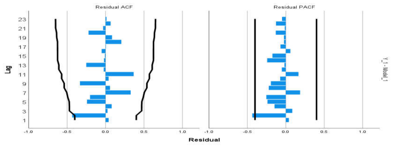
Figure 2.
Observed vs. Fitted Values.
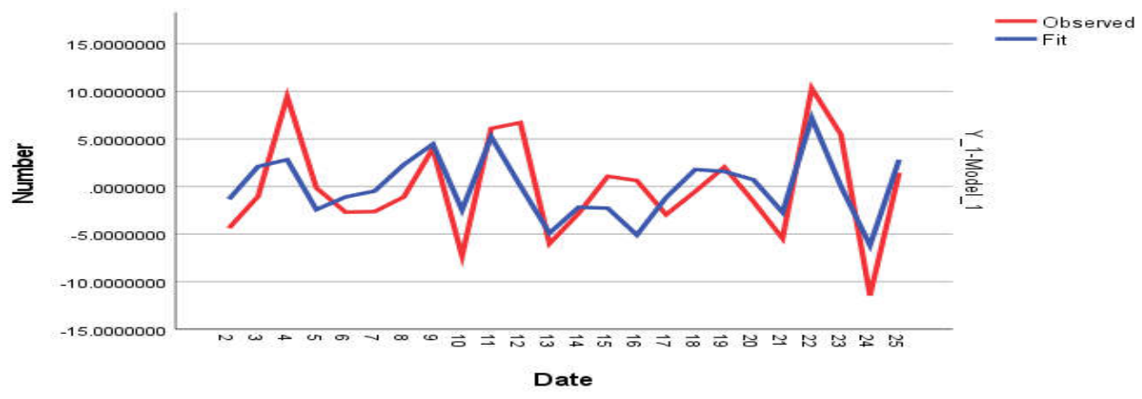

Table 1.
Study Data.
| Year | GDP_Value | GDP_Growth | Internet_Users | Gov_Expenditure_%GDP | Inflation | Patents | Patents (After Processing) |
|---|---|---|---|---|---|---|---|
| 2000 | 3.60E+11 | 4.718134 | 68.16645 | 25.86308 | -1.125 | 76 | 76 |
| 2001 | 3.61E+11 | 0.344593 | 63.56058 | 27.32667 | -1.12095 | 46 | 46 |
| 2002 | 3.59E+11 | -0.68839 | 64.5928 | 25.95096 | 0.247186 | 61 | 61 |
| 2003 | 3.90E+11 | 8.768734 | 69.83117 | 24.48451 | 0.612195 | 56 | 56 |
| 2004 | 4.24E+11 | 8.631005 | 75.08284 | 22.8591 | 0.515508 | 81 | 81 |
| 2005 | 4.49E+11 | 5.944896 | 81.95408 | 21.34028 | 0.479232 | 119 | 119 |
| 2006 | 4.64E+11 | 3.313485 | 89.9446 | 22.03925 | 2.209023 | 119 | 119 |
| 2007 | 4.74E+11 | 2.213654 | 94.86332 | 20.66207 | 4.167824 | 128 | 128 |
| 2008 | 5.04E+11 | 6.237988 | 96.10263 | 17.70425 | 9.870248 | 181.33 | |
| 2009 | 4.98E+11 | -1.06672 | 84.85834 | 22.18701 | 5.057223 | 234.67 | |
| 2010 | 5.23E+11 | 5.039515 | 82.54969 | 20.20287 | 5.339417 | 288 | 288 |
| 2011 | 5.85E+11 | 11.75882 | 84.35943 | 19.8723 | 5.826216 | 347 | 347 |
| 2012 | 6.19E+11 | 5.761574 | 81.74068 | 20.1587 | 2.86627 | 419 | |
| 2013 | 6.37E+11 | 2.945638 | 80.2515 | 22.36103 | 3.511042 | 491 | 491 |
| 2014 | 6.63E+11 | 4.024672 | 78.00011 | 25.59519 | 2.241853 | 652 | 652 |
| 2015 | 6.93E+11 | 4.655123 | 67.10527 | 28.91473 | 1.222693 | 715 | 715 |
| 2016 | 7.05E+11 | 1.704047 | 57.92166 | 24.83838 | 2.053471 | 1070 | 1070 |
| 2017 | 7.14E+11 | 1.182107 | 59.53198 | 23.3805 | -0.83485 | 909 | 909 |
| 2018 | 7.37E+11 | 3.226951 | 59.10291 | 23.1694 | 2.465943 | 1078 | 1078 |
| 2019 | 7.49E+11 | 1.651589 | 56.79382 | 22.67679 | -1.19299 | 1188 | 1188 |
| 2020 | 7.20E+11 | -3.80479 | 47.53316 | 27.37111 | 3.37235 | 1294 | 1294 |
| 2021 | 7.67E+11 | 6.519597 | 50.88393 | 21.67358 | 3.06329 | 1398 | 1398 |
| 2022 | 8.59E+11 | 12.00059 | 56.82416 | 19.13909 | 2.474074 | 1502 | |
| 2023 | 8.64E+11 | 0.542592 | 54.16901 | 20.93371 | 2.327085 | 1606 | |
| 2024 | 8.81E+11 | 1.996502 | 54.67871 | 21.32244 | 1.687921 | 1710 |
Source: World Bank (WDI), International Monetary Fund (IMF), International Telecommunication Union (ITU), World Intellectual Property Organization (WIPO), and compiled by the author.
Table 2.
Model Fit Statistics.
| Model Fit | |||||||||||
|---|---|---|---|---|---|---|---|---|---|---|---|
| Fit Statistic | Mean | SE | Minimum | Maximum | Percentile | ||||||
| 5 | 10 | 25 | 50 | 75 | 90 | 95 | |||||
| Stationary R-squared | .542 | . | .542 | .542 | .542 | .542 | .542 | .542 | .542 | .542 | .542 |
| R-squared | .542 | . | .542 | .542 | .542 | .542 | .542 | .542 | .542 | .542 | .542 |
| RMSE | 4.144 | . | 4.144 | 4.144 | 4.144 | 4.144 | 4.144 | 4.144 | 4.144 | 4.144 | 4.144 |
| MAPE | 208.164 | . | 208.164 | 208.164 | 208.164 | 208.164 | 208.164 | 208.164 | 208.164 | 208.164 | 208.164 |
| MaxAPE | 1658.940 | . | 1658.940 | 1658.940 | 1658.940 | 1658.940 | 1658.940 | 1658.940 | 1658.940 | 1658.940 | 1658.940 |
| MAE | 2.946 | . | 2.946 | 2.946 | 2.946 | 2.946 | 2.946 | 2.946 | 2.946 | 2.946 | 2.946 |
| MaxAE | 6.640 | . | 6.640 | 6.640 | 6.640 | 6.640 | 6.640 | 6.640 | 6.640 | 6.640 | 6.640 |
| Normalized BIC | 3.770 | . | 3.770 | 3.770 | 3.770 | 3.770 | 3.770 | 3.770 | 3.770 | 3.770 | 3.770 |
As shown in Table 2, the R-squared value suggests that the model explains approximately 54.2% of the variation in the dependent variable.
Table 3.
Model Statistics. Table 3 reports the model statistics, including the Ljung–Box Q test results and diagnostic indicators.
Table 3.
Model Statistics. Table 3 reports the model statistics, including the Ljung–Box Q test results and diagnostic indicators.
| Model Statistics | |||||||
|---|---|---|---|---|---|---|---|
| Model | Number of Predictors | Model Fit Statistics | Ljung-Box Q(18) | Number of Outliers | |||
| Stationary R-squared | Normalized BIC | Statistics | DF | Sig. | |||
| DIFF(Y,1)-Model_1 | 4 | .542 | 3.770 | 32.246 | 16 | .009 | 0 |
Table 4.
ARIMA Model Parameters.
| ARIMA Model Parameters | ||||||||
|---|---|---|---|---|---|---|---|---|
| Estimate | SE | t | Sig. | |||||
| DIFF(Y,1)-Model_1 | DIFF(Y,1) | No Transformation | Constant | -.163 | .646 | -.252 | .804 | |
| AR | Lag 1 | .185 | .341 | .544 | .594 | |||
| MA | Lag 1 | .999 | 39.388 | .025 | .980 | |||
| DIFF(X1,1) | No Transformation | Numerator | Lag 0 | -.023 | .202 | -.116 | .909 | |
| DIFF(X2,1) | No Transformation | Numerator | Lag 0 | -.867 | .463 | -1.873 | .078 | |
| DIFF(X3,1) | No Transformation | Numerator | Lag 0 | -.104 | .514 | -.203 | .842 | |
| DIFF(X4,1) | No Transformation | Numerator | Lag 0 | .000 | .011 | .025 | .980 | |
Table 5.
Descriptive Statistics.
| Descriptive Statistics | |||
|---|---|---|---|
| Mean | Std. Deviation | N | |
| DIFF(Y,1) | -.113401333 | 5.2650996966 | 24 |
| DIFF(X1,1) | -.561989167 | 5.5420302872 | 24 |
| DIFF(X2,1) | -.189193333 | 2.5983653792 | 24 |
| DIFF(X3,1) | .117205042 | 2.3899414925 | 24 |
| DIFF(X4,1) | 68.08 | 91.231 | 24 |
Table 6.
Correlations.
| Correlations | ||||||
|---|---|---|---|---|---|---|
| DIFF(Y,1) | DIFF(X1,1) | DIFF(X2,1) | DIFF(X3,1) | DIFF(X4,1) | ||
| Pearson Correlation | DIFF(Y,1) | 1.000 | .440 | -.578 | .186 | -.045 |
| DIFF(X1,1) | .440 | 1.000 | -.549 | .190 | -.387 | |
| DIFF(X2,1) | -.578 | -.549 | 1.000 | -.162 | -.078 | |
| DIFF(X3,1) | .186 | .190 | -.162 | 1.000 | .144 | |
| DIFF(X4,1) | -.045 | -.387 | -.078 | .144 | 1.000 | |
| Sig. (1-tailed) | DIFF(Y,1) | . | .016 | .002 | .192 | .416 |
| DIFF(X1,1) | .016 | . | .003 | .187 | .031 | |
| DIFF(X2,1) | .002 | .003 | . | .225 | .358 | |
| DIFF(X3,1) | .192 | .187 | .225 | . | .251 | |
| DIFF(X4,1) | .416 | .031 | .358 | .251 | . | |
| N | DIFF(Y,1) | 24 | 24 | 24 | 24 | 24 |
Table 7.
Model Summary.
| Model Summaryb | ||||||||||
|---|---|---|---|---|---|---|---|---|---|---|
| Model | R | R Square | Adjusted R Square | Std. Error of the Estimate | Change Statistics | |||||
| R Square Change | F Change | df1 | df2 | Sig. F Change | ||||||
| 1 | .602a | .363 | .229 | 4.6245455312 | .363 | 2.703 | 4 | 19 | .062 | 2.066 |
|
a. Predictors: (Constant), DIFF(X4,1), DIFF(X2,1), DIFF(X3,1), DIFF(X1,1) |
||||||||||
| b. Dependent Variable: DIFF(Y,1) | ||||||||||
Table 8.
Analysis of Variance (ANOVA).
| ANOVAa | ||||||
|---|---|---|---|---|---|---|
| Model | Sum of Squares | df | Mean Square | F | Sig. | |
| 1 | Regression | 231.247 | 4 | 57.812 | 2.703 | .062b |
| Residual | 406.342 | 19 | 21.386 | |||
| Total | 637.589 | 23 | ||||
a. Dependent Variable: DIFF(Y,1). b. Predictors: (Constant), DIFF(X4,1), DIFF(X2,1), DIFF(X3,1), DIFF(X1,1).
Table 9.
Coefficients.
| Coefficients | |||||||
|---|---|---|---|---|---|---|---|
| Model | Unstandardized Coefficients | Standardized Coefficients | t | Sig. | Correlations | ||
| B | Std. Error | Beta | Zero-order | ||||
| 1 | (Constant) | -.079 | 1.217 | -.065 | .949 | ||
| DIFF(X1,1) | .128 | .249 | .135 | .515 | .613 | .440 | |
| DIFF(X2,1) | -1.000 | .480 | -.493 | -2.083 | .051 | -.578 | |
| DIFF(X3,1) | .191 | .423 | .087 | .451 | .657 | .186 | |
| DIFF(X4,1) | -.003 | .013 | -.044 | -.201 | .843 | -.045 | |
Table 10.
Coefficients.
| Coefficientsa | |||||
|---|---|---|---|---|---|
| Model | Correlations | ||||
| Partial | Part | Tolerance | VIF | ||
| 1 | (Constant) | ||||
| DIFF(X1,1) | .117 | .094 | .486 | 2.056 | |
| DIFF(X2,1) | -.431 | -.382 | .598 | 1.671 | |
| DIFF(X3,1) | .103 | .083 | .908 | 1.101 | |
| DIFF(X4,1) | -.046 | -.037 | .690 | 1.448 | |
a. Dependent Variable: DIFF(Y,1).
Table 11.
Coefficient Correlations.
| Coefficientsa | |||||
|---|---|---|---|---|---|
| Model | Correlations | ||||
| Partial | Part | Tolerance | VIF | ||
| 1 | (Constant) | ||||
| DIFF(X1,1) | .117 | .094 | .486 | 2.056 | |
| DIFF(X2,1) | -.431 | -.382 | .598 | 1.671 | |
| DIFF(X3,1) | .103 | .083 | .908 | 1.101 | |
| DIFF(X4,1) | -.046 | -.037 | .690 | 1.448 | |
a. Dependent Variable: DIFF(Y,1).
Table 12.
Collinearity Diagnostics.
| Collinearity Diagnosticsa | ||||||||
|---|---|---|---|---|---|---|---|---|
| Model | Dimension | Eigenvalue | Condition Index | Variance Proportions | ||||
| (Constant) | DIFF(X1,1) | DIFF(X2,1) | DIFF(X3,1) | |||||
| 1 | 1 | 1.782 | 1.000 | .09 | .08 | .02 | .00 | |
| 2 | 1.588 | 1.059 | .05 | .06 | .15 | .10 | ||
| 3 | .888 | 1.416 | .04 | .02 | .07 | .81 | ||
| 4 | .524 | 1.844 | .45 | .18 | .32 | .01 | ||
| 5 | .218 | 2.860 | .36 | .67 | .44 | .08 | ||
| a. Dependent Variable: DIFF(Y,1) | ||||||||
Table 13.
Residual Statistics.
| Residuals Statisticsa | |||||
|---|---|---|---|---|---|
| Minimum | Maximum | Mean | Std. Deviation | N | |
| Predicted Value | -7.057822227 | 5.721476555 | -.113401333 | 3.1708407519 | 24 |
| Residual | -8.9507188797 | 7.3149576187 | .0000000000 | 4.2032182600 | 24 |
| Std. Predicted Value | -2.190 | 1.840 | .000 | 1.000 | 24 |
| Std. Residual | -1.935 | 1.582 | .000 | .909 | 24 |
Table 14.
Hypotheses and Final Decision (Publish-Ready).
| Hypothesis | Empirical Conclusion (2000–2024) | Decision |
|---|---|---|
| H1 | No statistically significant short-run effect is observed for most AI investment indicators. | Fail to reject the null hypothesis |
| H1a / H1b | No significant positive short-run impact is found for expenditure or patent indicators. | Alternative hypothesis rejected |
| H2 | One indicator shows marginal significance with a transitional (negative) effect. | Partially accepted (10% significance level) |
| H3 | The relationship cannot be fully determined using first differences and requires testing within the ARDL framework. | Likely to be accepted |
| H4 | ARIMAX demonstrates better in-sample fit but does not outperform in forecasting performance. | Partially accepted |
Disclaimer/Publisher’s Note: The statements, opinions and data contained in all publications are solely those of the individual author(s) and contributor(s) and not of MDPI and/or the editor(s). MDPI and/or the editor(s) disclaim responsibility for any injury to people or property resulting from any ideas, methods, instructions or products referred to in the content. |
© 2026 by the authors. Licensee MDPI, Basel, Switzerland. This article is an open access article distributed under the terms and conditions of the Creative Commons Attribution (CC BY) license (http://creativecommons.org/licenses/by/4.0/).
Copyright: This open access article is published under a Creative Commons CC BY 4.0 license, which permit the free download, distribution, and reuse, provided that the author and preprint are cited in any reuse.