

Submitted:
04 August 2026
Posted:
04 August 2026
You are already at the latest version
Abstract
Intelligent systems deployed in smart cities, smart grids, environmental monitoring, and other data-driven applications increasingly depend on reliable multivariate time-series forecasting. Recent deep forecasting models have achieved strong performance on various benchmarks, but their final predictions are often generated through a fixed forecast-generation process. This one-size-fits-all approach may be suboptimal because input windows exhibit different values, trends, and periodic patterns. We propose gap-aware residual selection (GARS), a plug-in refinement module for time-series forecasting that improves the prediction ability of an existing forecasting model rather than replacing it. GARS constructs deterministic reference forecasts from the observed input window and uses the differences between these forecasts and the initial forecast of the model as gap-aware residual information. Using only the observed input window and initial forecast, GARS constructs three component forecasts: the initial forecast, a gap-aware residual component that adjusts the initial forecast using these reference differences, and a direct residual component learned from the input window. The final forecast is obtained by assigning soft weights to the components across different segments of the forecast horizon rather than using fixed combinations. Future target values are used exclusively for training and evaluation and not for constructing reference forecasts, residuals, or soft weights. Experiments on five multivariate benchmark datasets related to energy, environment, electricity, traffic, and finance, using four representative forecasting models, show that GARS consistently improves average forecasting performance, reducing the mean squared error by 7.95% on average compared with the original models.
Keywords:
conditional weighting
; forecast refinement
; intelligent systems
; long-term forecasting
; residual correction
; time-series forecasting
1. Introduction
Time series forecasting (TSF) supports decision making across a wide range of intelligent-system domains [1,2], including smart cities, smart grids, environmental monitoring, and traffic management [3,4,5]. It is also applied to energy load planning [6], financial risk assessment [7], supply-chain and logistics planning [8], and healthcare monitoring [9,10]. Many forecasting models first encode the observed input window into a latent representation and then use a fixed forecasting function to generate predictions over the forecast horizon [11,12,13,14,15]. However, the observed input window used for forecasting may contain contextual cues about the future behavior of the series, including local trends, recent deviations, and level shifts [12,16,17]. Therefore, relying on a fixed forecasting function can limit the model’s ability to capture context-dependent dynamics. This limitation motivates forecasting models to adapt the prediction process according to the observed input window [2,17].
Recent advancements in TSF research have substantially improved forecasting accuracy through diverse model architectures, including recurrent models, attention-based Transformers, patch-based designs, multilayer perceptron (MLP)-style forecasters, and temporal convolution networks [11,12,13,14,15,18,19,20,21]. Complementary approaches further improve forecasting robustness by decomposing temporal patterns, addressing non-stationarity, or normalizing distribution shifts in the input window [16,17,22,23]. Collectively, these studies demonstrate that forecasting accuracy can be improved by changing model architectures or incorporating correction mechanisms into the forecasting model. In this study, we focus on refining the final prediction based on the observed input window after the base model produces an initial forecast, while preserving the base model itself. Unlike approaches that combine multiple trained models or rescale outputs after prediction, gap-aware residual selection (GARS) reuses a single base model and derives its correction from the gap between simple reference forecasts and that model’s initial forecast.
GARS is a plug-in module for time-series forecasting that refines the initial prediction of an existing TSF model rather than replacing the model itself. GARS first computes a small set of deterministic reference forecasts from the observed input window. Each one extrapolates a simple input-derived behavior, such as a recent value, a trend, or a repeated temporal pattern. The difference between each reference forecast and the initial forecast provides a gap signal indicating the deviation of the base model’s initial forecast from the reference forecasts. Here, “gap” denotes a forecast discrepancy rather than missing observations or irregular sampling intervals. Using the gap signal together with the input window, GARS constructs three component forecasts: the initial forecast itself, a gap-aware residual component that adjusts the initial forecast using these discrepancies, and a direct residual component learned from the observed input window. The final prediction is obtained by combining these components through soft weighting.
The proposed design is modular because it can be applied to an existing forecasting model without changing the internal architecture. Given an input window and an initial forecast generated by the base model, GARS forms three component forecasts that are used to generate the final prediction. Ground-truth future values in the forecast horizon are used exclusively to compute the training loss and evaluation metrics. They are not used to compute reference forecasts, residual components, or soft weights. Therefore, the refinement process does not use future information that would be unavailable at inference time. GARS assigns soft weights over different parts of the forecast horizon to combine the initial forecast, a gap-aware residual component, and a direct residual component. This approach allows the contribution of each component forecast to vary across different segments of the forecast horizon while preserving the base forecasting architecture. We hypothesize that the gap signal exposes systematic, horizon-localized biases of the base model relative to simple interpretable extrapolations. Because the gap already encodes the base model’s output, a small module can use it directly, whereas a residual predictor that sees only the input would first have to relearn the base model’s behavior to obtain the same information.
In our experiments, GARS is integrated with four TSF models: PatchTST [14], iTransformer [15], TimeMixer [20], and TimesNet [24], and changes in performance relative to the initial forecasts are evaluated. The benchmarks encompass multivariate time-series datasets spanning the solar energy, weather, electricity consumption, traffic, and exchange-rate domains, and the forecasting errors are reduced on average using the proposed module. We summarize our contributions as follows. First, we propose GARS, a plug-in module that adjusts the final prediction using only the input window and initial forecast from the base model. Second, we design a gap-aware residual construction that uses the difference between reference forecasts and the initial forecast as a correction signal. Third, we evaluate the proposed module across multiple TSF models and multivariate benchmarks, showing that it can improve average forecasting performance without requiring a new standalone forecasting model.
2. Related Work
2.1. Base Forecasting Models
Recent TSF research has led to the development of various base forecasting models. Transformer-based models have been used to capture long-range dependencies and cross-variate interactions, whereas patch-based designs aim to improve efficiency and representation capacity by processing long input windows into more compact units [13,14,25]. Inverted representation designs, such as iTransformer, use variable-level information more directly in the forecasting process rather than relying only on conventional time-axis-centered representations [15,26]. Linear, MLP-style, and mixer-style models employ comparatively simple projection or mixing operations across the time and channel dimensions, yet remain competitive in long-horizon forecasting settings [18,19,20,27,28]. Periodicity- or temporal-variation-oriented models, such as TimesNet, focus on capturing repetitive patterns and multiperiod structures in time series [21,24,29]. Because these base models encode different inductive biases, their relative performance can vary across datasets, forecast horizons, numbers of variables, and input lengths. This study does not propose another base forecasting model; instead, it designs a plug-in module that adjusts the final prediction after the base model produces the initial forecast.
2.2. Forecast Refinement Without Replacing Base Models
A related line of work improves forecasting without designing an entirely new base model. Normalization-based methods normalize the input window with instance-level statistics and reverse this normalization on the output, reducing non-stationary scale and mean shifts between the input window and the forecast horizon [16]. Decomposition-aware and frequency-aware methods improve forecasts by separating or using structured components, such as trends, seasonality, and frequency information [22,23]. Stationarity-aware and model-agnostic enhancement methods further aim to improve forecasting behavior across different base models without committing to a specific forecasting architecture [17,30,31]. These studies show that forecasting performance can be improved through input transformations, structured decomposition, or additional correction mechanisms without fully replacing the base forecasting model.
Output-level refinement is also relevant to the present study because it modifies or corrects the forecast after the initial prediction becomes available. Post-hoc revision methods, such as post-hoc instance-aware revision, improve generated forecasts using contextual information or instance-level diagnostics [32]. These methods demonstrate that substantial improvements can be obtained at the prediction level without redesigning the forecasting model. GARS is similar to these methods in that it starts from an initial forecast, but it differs fundamentally in how the correction is learned and constructed. GARS is trained with the base model as a plug-in module, and its correction components are constructed from the input window and initial forecast rather than from failure-case detection or similar-instance retrieval.
2.3. Objective-Level Forecasting Enhancements
Some studies improve forecasting performance by changing the training objective instead of modifying the model architecture or applying output-level corrections. For example, the Soft-DTW loss uses a differentiable form of dynamic time warping to account for temporal alignment between predicted and ground-truth sequences [33]. The DILATE loss (DIstortion Loss including shApe and TimE) combines shape and temporal distortion terms; therefore, training is not limited to comparing predictions and ground truth at matching time steps [34]. Recent objective-level methods further use decomposition-aware supervision or label-output alignment to address imbalanced learning signals or distributional differences in long-horizon forecasting [35,36,37]. These approaches show that forecasting behavior can change depending on the training objective, even when the model architecture is fixed. Unlike objective-level methods, GARS does not introduce a new loss function. Instead, it adjusts the final prediction after the base model generates an initial forecast under a standard forecasting loss.
2.4. Conditional Weighting and Soft Mixing
Conditional weighting and soft mixing methods adjust the contribution of model components according to the input instance. Mixture-of-experts and conditional computation methods select or weight different experts or submodules, enabling different inputs to follow distinct computational pathways [38,39,40]. In TSF, methods such as Pathformer similarly adjust internal computation by selecting scales, patches, or representations according to the input time series [41,42]. These studies have shown that input-dependent computation can be used for forecasting. However, they mainly focus on choosing experts, scales, or representations within the forecasting model before the final forecast is produced. GARS adopts the broader concept of input-dependent weighting but applies it after the base model generates an initial forecast rather than incorporating it within the base forecasting architecture.
3. Methods
3.1. Problem Formulation and Plug-In Forecast Refinement
We define the multivariate long-horizon forecasting problem and the plug-in refinement structure of GARS. Let the input window be , where B is the batch size, L is the input length, and C is the number of variables. The target horizon to be predicted is denoted by , where H is the forecast horizon length. The base forecasting model takes the input window and produces an initial forecast . GARS then uses the input window and initial forecast together to produce the final prediction :
After the base model produces the initial forecast , GARS uses the input window and initial forecast to construct additional component forecasts and soft weights for the final combination. The module retains as one component forecast and derives a descriptor and reference forecasts from the input window to construct the additional component forecasts. From the same descriptor, it computes soft weights that determine the contribution of each component forecast to the final prediction. The component forecasts are then combined with these soft weights to produce the final prediction . In this way, GARS adjusts how the final prediction is formed without modifying the internal architecture of the base model. Figure 1 summarizes the resulting data flow from the input window and initial forecast to the final prediction.
3.2. Model Details and Component Forecast Construction
GARS constructs three component forecasts from the initial forecast without changing the internal architecture of the base model . It uses a descriptor and reference forecasts computed from the input window, together with three small MLP modules. The descriptor summarizes the input window, the reference forecasts provide gap information, and the MLPs produce the component forecasts used for the final prediction.
GARS first summarizes the input window into a descriptor . The descriptor concatenates ten channel-wise summaries of the input window. These summaries include the full-window mean and standard deviation, summaries from the early and late parts of the window, differenced summaries, coarse reconstruction residual magnitude, last-to-recent-mean deviation, and curvature magnitude. Here, q is the length of the early and late parts of the input window, defined as one-quarter of L rounded down, with a minimum of two steps. The operator denotes temporal differencing, and denotes a coarse reconstruction obtained by average pooling over length-4 temporal windows and linearly interpolating the pooled sequence back to length L. The descriptor uses the following ten channel-wise components in the indicated concatenation order.
| No. | Summary | Expression |
| 1 | Full mean | |
| 2 | Full standard deviation | |
| 3 | Late-window mean | |
| 4 | Early-window mean | |
| 5 | Late-window standard deviation | |
| 6 | Difference mean | |
| 7 | Difference standard deviation | |
| 8 | Coarse residual magnitude | |
| 9 | Last-to-recent-mean deviation | |
| 10 | Curvature magnitude |
The operators and denote the time-axis mean and standard deviation computed separately for each channel. All descriptor entries are deterministic functions of the input window and contain no trainable parameters.
GARS then constructs four deterministic reference forecasts from the input window: the last-value, trend, repeated-period, and smoothed-trend forecasts. Each reference forecast extrapolates the corresponding simple pattern from the input window into the forecast horizon using a fixed rule, rather than relying on a separately trained forecasting model. Let and denote the first and last time steps of the input window, and let denote the forecast step. The repeated-period forecast uses a period , and the smoothed-trend forecast uses a moving-average window ; both are clamped so that neither exceeds the input length L. Here, denotes the input window after applying a centered moving average with window size k, computed via average pooling with edge padding of so that the smoothed sequence retains length L. GARS defines each one as follows.
| No. | Reference forecast | Definition |
| 1 | Last-value | |
| 2 | Trend | |
| 3 | Repeated-period | |
| 4 | Smoothed-trend |
For , the term makes the repeated-period forecast cycle through the last P observed steps. The smoothed-trend forecast applies the trend rule to the smoothed input window rather than to . All four reference forecasts are deterministic functions of the input window and contain no trainable parameters.
Let denote the four reference forecasts stacked along a new axis. The gap residual bank then collects the differences between these reference forecasts and the initial forecast :
where is broadcast along this axis. The gap residual bank does not represent the error between the ground-truth future values and the initial forecast. It represents only discrepancies between the reference forecasts and the initial forecast. Therefore, the ground-truth target horizon is not used when constructing the reference forecasts or the gap residual bank.
GARS uses the descriptor and gap residual bank to construct three component forecasts. The first component is the initial forecast itself. The second component adjusts the initial forecast using a residual direction obtained from the gap residual bank. The gap coefficient MLP maps the descriptor to bounded channel-wise coefficients for the four reference residuals, and their weighted sum becomes the gap-aware residual . The third component adds a direct residual , which the direct residual MLP produces from the same descriptor. Both MLPs have two layers with hidden width 64. The block-wise weighting MLP is introduced below.
With the fixed residual damping scale , the three component forecasts in are defined as
The shared constant is a fixed residual damping hyperparameter applied to both residual components, not a learned scale parameter.
3.3. Block-Wise Soft Weighting
After constructing the three component forecasts, GARS determines how to combine them over the forecast horizon. GARS partitions the forecast horizon into four contiguous blocks, which we refer to as forecast-horizon blocks. It then computes three soft weights for each block, one for each component forecast. All forecast steps within a block share these weights. This design allows the contribution of each component forecast to vary across different parts of the forecast horizon rather than using the same mixture for the entire horizon.
The block-wise weighting module receives the descriptor and produces three scores for each forecast-horizon block, one for each component forecast. A softmax over the three scores provides block-specific weights. For a forecast step in block b, the final prediction is the weighted sum of , , and using the weights for block b. Because the weighting module uses only the descriptor from the input window, the weights are computed without observing the ground-truth target horizon. During inference, the weights are recomputed for each input window, whereas the learned parameters of the weighting module remain fixed. Figure 2 illustrates this block-wise weighting process.
3.4. Training and Inference Details
GARS follows the same scaling convention as the base model for the input windows, initial forecasts, and target horizons used during training. In the reported experiments, the lookback length was set to . The scaling statistics and the scale at which metrics are computed follow the experimental setup in Section 4.
The trainable modules of GARS are limited to three compact MLPs: the gap coefficient MLP, direct residual MLP, and block-wise weighting MLP. Each MLP uses layer normalization [43], a hidden layer of width 64, a Gaussian error linear unit (GELU) nonlinearity [44], and a task-specific linear output layer. The three MLPs do not share parameters, and their output dimensions differ according to the target quantity. Table 1 summarizes the module configurations used in the reported experiments.
The residual damping coefficient is fixed at for both the gap-aware residual component and the direct residual component in all main experiments. We analyze the sensitivity to this coefficient in Section 4.3.
We use the standard mean squared error (MSE) forecasting objective:
The full system was trained end-to-end using this objective. Optimization used AdamW [45] over the full parameter set, including both the base model and GARS. The base model parameters were not frozen. No additional loss terms were used. Thus, GARS changes only how the final prediction is formed while retaining the same training objective as the base model. Table 2 summarizes the shared training settings.
During inference, the ground-truth target horizon is unavailable. Therefore, GARS computes the descriptor, reference forecasts, component forecasts, and block-wise weights using only the input window, initial forecast, and learned parameters. The ground-truth target horizon is used only for the training loss and evaluation metrics. Computing the descriptor and the reference forecasts involves no trainable parameters.
4. Experimental Results
4.1. Experimental Setup
4.1.1. Datasets
The evaluation used five application-oriented multivariate long-term forecasting benchmark datasets: Solar, Weather, Electricity, Traffic, and Exchange. These cover renewable energy monitoring, environmental sensing, smart grid demand forecasting, traffic management, and exchange-rate forecasting, respectively. Among them, Solar, Electricity, Traffic, and Exchange datasets follow the LSTNet benchmark setting [3], while the Weather dataset follows the long-term forecasting benchmark setting used in Autoformer [22]. Following common long-term forecasting protocols, the lookback length was fixed at and the reported forecast horizons were . We split each dataset into training, validation, and test subsets with a 7:1:2 ratio. Table 3 summarizes the dataset statistics used in the main experiments.
4.1.2. Base Forecasting Models and Paired Comparison Protocol
We evaluated GARS using four base forecasting models: iTransformer, PatchTST, TimeMixer, and TimesNet. These models represent diverse architectural paradigms. Specifically, iTransformer uses an inverted representation design, PatchTST adopts patch-based Transformer forecasting, TimeMixer performs forecasting through temporal mixing, and TimesNet models transformed temporal patterns. The purpose of this evaluation is to demonstrate that GARS can be integrated with a wide range of forecasting architectures rather than to introduce a new standalone forecasting model.
We conducted paired comparisons for all combinations of datasets, forecast horizons, and base models. The model trained without GARS is referred to as the original model, and the same model equipped with GARS is referred to as the GARS version. To ensure a controlled comparison, the two versions used the same data splits, forecasting setting, training protocol, and evaluation procedure. The only architectural difference is that the GARS-equipped version refines the initial forecast using the component construction and block-wise weighting described in Section 3.2 and Section 3.3. GARS and the base model were trained jointly under the same MSE forecasting objective. The base model parameters were updated during training, and no separate pretraining stage was used.
4.1.3. Training and Evaluation Details
We report MSE and mean absolute error (MAE) on the test set. We also assess statistical significance using a Wilcoxon signed-rank test over the paired results from the 80 configurations. Scaling statistics were computed only from the training set and then applied to the validation and test sets. We did not convert the values back to the original scale before computing the reported metrics. All models were trained end-to-end using MSE loss. We used AdamW with a learning rate of , a weight decay of 0, and gradient clipping of . For each run, training proceeded for a fixed number of epochs, and the checkpoint with the lowest validation MSE was evaluated on the test set.
The main application experiments included 80 combinations of datasets, base models, and forecast horizons. Unless otherwise noted, each configuration used a lookback length , seeds 43, 44, and 45, at most 1024 samples, a batch size of 32, and 8 epochs. All experiments were conducted on a single NVIDIA GeForce RTX 3090 GPU.
4.2. Main Forecasting Results
Table 4 presents the main forecasting results from the paired comparison between the original model and the GARS version. For each combination of dataset, forecast horizon, and base model, the table reports the three-seed average MSE and MAE values. The better value in each paired comparison is highlighted in bold.
Across the 80 evaluation settings, GARS reduced the MSE in 65 of them. Among these MSE-winning settings, 61 showed relative reductions greater than . Averaged over all 80 settings, the mean relative reduction in MSE was . The strongest gains were observed for Solar, Electricity, and Exchange. Weather showed smaller but mostly positive gains, whereas Traffic yielded mixed results, particularly for TimesNet. MAE improved in 45 of the 80 settings. Table 5 reports a Wilcoxon signed-rank test of these paired improvements. The MSE reduction is highly significant overall () and holds on every dataset except Traffic, indicating that the average gain is not driven by a few settings. In contrast, the MAE improvement is not significant overall and is significantly negative on Weather, consistent with its smaller and less consistent gains.
Figure 3 complements Table 4 by showing the distribution of relative MSE improvements. Each point corresponds to a combination of dataset, forecast horizon, and base model. Positive values indicate that GARS obtains a lower MSE than the original model. The distribution is mostly positive for all four base models, whereas the dataset-level patterns vary more. Solar shows the largest overall improvement; Weather, Electricity, and Exchange are mostly positive, whereas Traffic includes several near-zero or negative cases.
Table 6 summarizes the main evaluation settings by forecast horizon. Each horizon includes 20 evaluation settings corresponding to five datasets and four base models. The mean relative MSE improvement is positive for all four horizons. The largest mean MSE improvement is observed at , whereas the smallest is observed at , where the mean MAE change also becomes negative. These findings indicate that the benefit of GARS extends across forecast horizons but becomes less consistent at the longest horizon.
4.3. Component Analysis
The component analysis examines how individual GARS components contribute to the observed forecasting gains. The component-removal ablation used a compact diagnostic setting with PatchTST, iTransformer, and TimeMixer on the Weather, Electricity, and Exchange datasets at horizons , using three random seeds. This setting was used to isolate the effect of each component within a controlled but smaller evaluation scope. In Table 7 and Table 8, relative improvements are computed against the original model, and positive values indicate lower error than the original model.
Table 7 and Table 8 compare full GARS with two variants that remove one correction component at a time. Removing the gap-aware residual component caused the largest performance reduction: the mean MSE improvement decreased from to , and the mean MAE improvement changed from to . Removing the direct residual component preserved a larger share of the gain, with a mean MSE improvement of and a mean MAE improvement of . These results indicate that the gap-aware residual component is the main contributor in this diagnostic setting, whereas the direct residual component provides an additional but smaller contribution.
The reference-forecast ablation further examines the reference forecasts used to construct the gap-aware residual component. To align this diagnostic with the main evaluation protocol, it used the Weather, Electricity, Traffic, and Exchange datasets with PatchTST, iTransformer, TimeMixer, and TimesNet at horizons over three seeds. Each variant removed one reference forecast while keeping the remaining GARS structure unchanged. Mean relative improvements were measured against the original model on the same matched evaluation set. V, T, R, and S denote the last-value, trend, repeated-period, and smoothed-trend forecasts, respectively.
Table 9 shows that the full set gave the best average MSE and MAE improvement on the matched evaluation set. Removing any single reference forecast lowered the overall mean improvement. The largest overall decrease occurred when the smoothed-trend forecast was removed, reducing mean MSE improvement from to . Removing the repeated-period forecast particularly weakened the result on Electricity, where the dataset-wise mean MSE improvement dropped from to . These results suggest that the reference forecasts provide complementary information rather than a single dominant source of improvement.
Finally, we evaluated sensitivity to the fixed residual damping coefficient . The same was applied to both the gap-aware residual component and the direct residual component. The analysis used the same compact diagnostic setting as the component-removal ablation. Table 10 reports relative improvements against the original model for this sensitivity analysis.
Table 10 shows that gave the best mean MSE improvement () and the best mean MAE improvement () among the tested values. Both smaller () and larger values gave lower average improvements. We therefore used as an empirical setting selected from the ablation, not as a learned or theoretically optimal value.
5. Discussion
The main results are consistent with the goal of GARS design as a plug-in forecast refinement module. GARS refines the initial forecast after it is produced by a base model rather than replacing the base forecasting architecture. The architecture is therefore preserved, although the base model parameters are still updated during joint training, as described in the experimental setup. Across the four tested base models, GARS consistently achieved a positive average reduction in MSE, suggesting that the observed gain was not limited to a single forecasting architecture.
Improvements in MAE are smaller than those in MSE, and the Traffic dataset exhibits greater variability in results than the other benchmarks. The Traffic dataset contains a large number of variables () and exhibits heterogeneous relationships among road sensors. However, the stronger gains observed on the Electricity dataset indicate that channel count alone is not a sufficient explanation. Therefore, the results on the Traffic dataset suggest dataset-specific challenges rather than a general limitation on high-dimensional benchmarks. On Traffic, the reported metrics for iTransformer and PatchTST are nearly identical between the original model and GARS. This is consistent with the block-wise weighting concentrating almost entirely on the initial-forecast component, so that the reference-based corrections had little effect for these two base models. These results indicate the broad applicability of GARS across datasets and base models, while also suggesting that the improvement is not consistent in every setting.
The component analyses provide further evidence regarding the sources of the improvements. In the component-removal ablation, removing the gap-aware residual component caused a larger performance reduction than removing the direct residual component. The reference-forecast ablation shows that the full set gave the best average improvement, and that removing individual reference forecasts weakened the result. The residual-damping analysis supports as an empirical setting in the tested range. Taken together, these findings suggest that GARS does not appear to rely on a single correction component or a single reference forecast. Instead, its gains are associated with combining discrepancies between the initial forecast and multiple reference forecasts through a controlled residual adjustment.
6. Conclusions
This paper presented GARS, a plug-in forecast refinement module for long-term time-series forecasting. To refine the initial forecast produced by a base model, GARS constructs reference forecasts from the input window and forms gap-aware and direct residual components. These components are adaptively combined using block-wise soft weights computed without ground-truth target values during inference. Experiments conducted on five multivariate benchmarks and four base models showed a positive average MSE improvement, with stronger gains for the Solar, Electricity, and Exchange datasets. The component analyses further showed that the gap-aware residual component, the full set of reference forecasts, and a moderate residual damping coefficient contribute to the observed improvements. However, the gains are not uniform: MAE improvements are smaller than MSE improvements, the Traffic dataset remains more variable than the other benchmarks, and some long-horizon settings are less consistent. Because GARS is also trained jointly with each backbone and adds a direct-residual output layer that scales with the horizon and the number of variables, we regard it as a promising but dataset-dependent refinement approach rather than a universally applicable one. Future work should examine more robust refinement strategies for dataset-specific cases such as Traffic and quantify the runtime and memory costs of the module in deployment-oriented settings.
Funding
The present research has been conducted by the Excellent Researcher Support Project of Kwangwoon University in 2026. This work was supported by the IITP(Institute of Information & Communications Technology Planning & Evaluation)-ITRC(Information Technology Research Center) grant funded by the Korea government(Ministry of Science and ICT)(IITP-2026- RS-2022-00156225).
References
- Lim, B.; Zohren, S. Time-series forecasting with deep learning: a survey. Philos. Trans. R. Soc. A 2021, 379, 20200209. [Google Scholar] [CrossRef] [PubMed]
- Benidis, K.; Rangapuram, S.S.; Flunkert, V.; Wang, Y.; Maddix, D.; Turkmen, C.; Gasthaus, J.; Bohlke-Schneider, M.; Salinas, D.; Stella, L.; et al. Deep Learning for Time Series Forecasting: Tutorial and Literature Survey. ACM Comput. Surv. 2022, 55. [Google Scholar] [CrossRef]
- Lai, G.; Chang, W.C.; Yang, Y.; Liu, H. Modeling long-and short-term temporal patterns with deep neural networks. In Proceedings of the The 41st international ACM SIGIR conference on research & development in information retrieval, 2018; pp. 95–104. [Google Scholar]
- Li, Y.; Yu, R.; Shahabi, C.; Liu, Y. Diffusion Convolutional Recurrent Neural Network: Data-Driven Traffic Forecasting. In Proceedings of the International Conference on Learning Representations, 2018. [Google Scholar]
- Yu, B.; Yin, H.; Zhu, Z. Spatio-Temporal Graph Convolutional Networks: A Deep Learning Framework for Traffic Forecasting. In Proceedings of the Twenty-Seventh International Joint Conference on Artificial Intelligence. International Joint Conferences on Artificial Intelligence Organization, 2018; pp. 3634–3640. [Google Scholar] [CrossRef] [PubMed]
- Zhao, Y. Research on Data Model Fusion Driven Dual End Uncertainty Source Load Probability Prediction and Its Application in New Energy Power Systems. IEIE Trans. Smart Process. Comput. 2025, 14, 389–399. [Google Scholar] [CrossRef]
- Zhang, B.; Tao, M. Design and Implementation of a Multi-factor Intelligent Mining System for Stocks Based on GA-TGCN. IEIE Trans. Smart Process. Comput. 2025, 14, 178–190. [Google Scholar] [CrossRef]
- Zhu, X. Application of Artificial Intelligence in the Problem of Agricultural Cold Chain Logistics Center Site Selection. IEIE Trans. Smart Process. Comput. 2025, 14, 535–544. [Google Scholar] [CrossRef]
- Chen, Y.; Liang, X.; Qi, P.; Xia, S.; Tong, J. Multimodal heart failure prediction model based on graph convolutional neural network. Biomed. Eng. Lett. 2026. [Google Scholar] [CrossRef]
- Fuadah, N.; Lim, K.M. Advances in cardiovascular signal analysis with future directions: a review of machine learning and deep learning models for cardiovascular disease classification based on ECG, PCG, and PPG signals. Biomed. Eng. Lett. 2025, 15, 619–660. [Google Scholar] [CrossRef]
- Salinas, D.; Flunkert, V.; Gasthaus, J.; Januschowski, T. DeepAR: Probabilistic Forecasting with Autoregressive Recurrent Networks. Int. J. Forecast. 2020, 36, 1181–1191. [Google Scholar] [CrossRef]
- Lim, B.; Arik, S.O.; Loeff, N.; Pfister, T. Temporal Fusion Transformers for Interpretable Multi-horizon Time Series Forecasting. Int. J. Forecast. 2021, 37, 1748–1764. [Google Scholar] [CrossRef]
- Zhou, H.; Zhang, S.; Peng, J.; Zhang, S.; Li, J.; Xiong, H.; Zhang, W. Informer: Beyond efficient transformer for long sequence time-series forecasting. Proc. Proc. AAAI Conf. Artif. Intell. 2021, Vol. 35, 11106–11115. [Google Scholar] [CrossRef]
- Nie, Y.; Nguyen, N.H.; Sinthong, P.; Kalagnanam, J. A Time Series is Worth 64 Words: Long-term Forecasting with Transformers. In Proceedings of the International Conference on Learning Representations, 2023. [Google Scholar]
- Liu, Y.; Hu, T.; Zhang, H.; Wu, H.; Wang, S.; Ma, L.; Long, M. iTransformer: Inverted Transformers Are Effective for Time Series Forecasting. In Proceedings of the International Conference on Learning Representations, 2024. [Google Scholar]
- Kim, T.; Kim, J.; Tae, Y.; Park, C.; Choi, J.H.; Choo, J. Reversible Instance Normalization for Accurate Time-Series Forecasting against Distribution Shift. In Proceedings of the International Conference on Learning Representations, 2022. [Google Scholar]
- Liu, Y.; Wu, H.; Wang, J.; Long, M. Non-stationary Transformers: Exploring the Stationarity in Time Series Forecasting. Proc. Adv. Neural Inf. Process. Syst. 2022, Vol. 35, 9881–9893. [Google Scholar] [CrossRef]
- Chen, S.A.; Li, C.L.; Arik, S.O.; Yoder, N.C.; Pfister, T. TSMixer: An All-MLP Architecture for Time Series Forecasting. Transactions on Machine Learning Research, 2023. [Google Scholar]
- Das, A.; Kong, W.; Leach, A.; Mathur, S.K.; Sen, R.; Yu, R. Long-term Forecasting with TiDE: Time-series Dense Encoder. Transactions on Machine Learning Research, 2023. [Google Scholar]
- Wang, S.; Wu, H.; Shi, X.; Hu, T.; Luo, H.; Ma, L.; Zhang, J.; ZHOU, J. TimeMixer: Decomposable Multiscale Mixing for Time Series Forecasting. In Proceedings of the International Conference on Learning Representations, 2024. [Google Scholar]
- Bai, S.; Kolter, J.Z.; Koltun, V. An empirical evaluation of generic convolutional and recurrent networks for sequence modeling. arXiv 2018, arXiv:1803.01271. [Google Scholar]
- Wu, H.; Xu, J.; Wang, J.; Long, M. Autoformer: Decomposition Transformers with Auto-Correlation for Long-Term Series Forecasting. Proc. Adv. Neural Inf. Process. Syst. 2021, Vol. 34, 22419–22430. [Google Scholar]
- Zhou, T.; Ma, Z.; Wen, Q.; Wang, X.; Sun, L.; Jin, R. Proceedings of the Proceedings of the 39th International Conference on Machine Learning. PMLR, 17–23 Jul 2022, Vol. 162, Proceedings of Machine Learning Research. 27268–27286.
- Wu, H.; Hu, T.; Liu, Y.; Zhou, H.; Wang, J.; Long, M. TimesNet: Temporal 2D-Variation Modeling for General Time Series Analysis. In Proceedings of the International Conference on Learning Representations, 2023. [Google Scholar]
- Liu, S.; Yu, H.; Liao, C.; Li, J.; Lin, W.; Liu, A.X.; Dustdar, S. Pyraformer: Low-Complexity Pyramidal Attention for Long-Range Time Series Modeling and Forecasting. In Proceedings of the International Conference on Learning Representations, 2022. [Google Scholar]
- Zhang, Y.; Yan, J. Crossformer: Transformer Utilizing Cross-Dimension Dependency for Multivariate Time Series Forecasting. In Proceedings of the International Conference on Learning Representations, 2023. [Google Scholar]
- Zeng, A.; Chen, M.; Zhang, L.; Xu, Q. Are transformers effective for time series forecasting? Proc. Proc. AAAI Conf. Artif. Intell. 2023, Vol. 37, 11121–11128. [Google Scholar] [CrossRef]
- Oreshkin, B.N.; Carpov, D.; Chapados, N.; Bengio, Y. N-BEATS: Neural basis expansion analysis for interpretable time series forecasting. In Proceedings of the International Conference on Learning Representations, 2020. [Google Scholar]
- Liu, M.; Zeng, A.; Chen, M.; Xu, Z.; Lai, Q.; Ma, L.; Xu, Q. SCINet: Time Series Modeling and Forecasting with Sample Convolution and Interaction. Proc. Adv. Neural Inf. Process. Syst. 2022, Vol. 35, 5816–5828. [Google Scholar] [CrossRef]
- Luo, D.; Wang, X. DecompNet: Enhancing Time Series Forecasting Models with Implicit Decomposition. Proc. Adv. Neural Inf. Process. Syst. 2025, Vol. 38, 32278–32317. [Google Scholar]
- Du, Y.; Wang, J.; Feng, W.; Pan, S.; Qin, T.; Xu, R.; Wang, C. AdaRNN: Adaptive Learning and Forecasting of Time Series. Proceedings of the 30th ACM International Conference on Information and Knowledge Management. Association for Computing Machinery 2021, CIKM ’21, 402–411. [Google Scholar] [CrossRef]
- Liu, Z.; Cheng, M.; Zhao, G.; Yang, J.; Liu, Q.; Chen, E. Improving Time Series Forecasting via Instance-aware Post-hoc Revision. Proc. Adv. Neural Inf. Process. Syst. 2025, Vol. 38, 35604–35629. [Google Scholar]
- Cuturi, M.; Blondel, M. Proceedings of the Proceedings of the 34th International Conference on Machine Learning. PMLR, 2017, Vol. 70, Machine Learning Research. 894–903.
- Le Guen, V.; Thome, N. Shape and Time Distortion Loss for Training Deep Time Series Forecasting Models. In Proceedings of the Advances in Neural Information Processing Systems, 2019; Curran Associates, Inc.; Vol. 32. [Google Scholar]
- Qiu, X.; Wu, X.; Cheng, H.; Liu, X.; Guo, C.; Hu, J.; Yang, B. DBLoss: Decomposition-based Loss Function for Time Series Forecasting. Proc. Adv. Neural Inf. Process. Syst. 2025, Vol. 38, 27741–27768. [Google Scholar]
- Wang, H.; Pan, L.; Chen, Z.; Chen, X.; Dai, Q.; Wang, L.; Li, H.; Lin, Z. Time-o1: Time-Series Forecasting Needs Transformed Label Alignment. In Proceedings of the Advances in Neural Information Processing Systems; Curran Associates, Inc., 2025; Vol. 38, pp. 8660–8690. [Google Scholar]
- Park, K.; Kim, J.; Lee, S. AliO: Output Alignment Matters in Long-Term Time Series Forecasting. Proc. Adv. Neural Inf. Process. Syst. 2025, Vol. 38, 119563–119608. [Google Scholar]
- Jacobs, R.A.; Jordan, M.I.; Nowlan, S.J.; Hinton, G.E. Adaptive Mixtures of Local Experts. Neural Comput. 1991, 3, 79–87. [Google Scholar] [CrossRef] [PubMed]
- Jordan, M.I.; Jacobs, R.A. Hierarchical Mixtures of Experts and the EM Algorithm. Neural Comput. 1994, 6, 181–214. [Google Scholar] [CrossRef]
- Shazeer, N.; Mirhoseini, A.; Maziarz, K.; Davis, A.; Le, Q.V.; Hinton, G.E.; Dean, J. Outrageously Large Neural Networks: The Sparsely-Gated Mixture-of-Experts Layer. In Proceedings of the International Conference on Learning Representations, 2017. [Google Scholar]
- Chen, P.; Zhang, Y.; Cheng, Y.; Shu, Y.; Wang, Y.; Wen, Q.; Yang, B.; Guo, C. Pathformer: Multi-scale Transformers with Adaptive Pathways for Time Series Forecasting. In Proceedings of the International Conference on Learning Representations, 2024. [Google Scholar]
- Wu, X.; Qiu, X.; Cheng, H.; Li, Z.; Hu, J.; Guo, C.; Yang, B. Enhancing Time Series Forecasting through Selective Representation Spaces: A Patch Perspective. In Proceedings of the Advances in Neural Information Processing Systems; Curran Associates, Inc., 2025; Vol. 38, pp. 23328–23354. [Google Scholar]
- Ba, J.L.; Kiros, J.R.; Hinton, G.E. Layer normalization. arXiv 2016, arXiv:1607.06450. [Google Scholar]
- Hendrycks, D.; Gimpel, K. Gaussian error linear units (gelus). arXiv 2016, arXiv:1606.08415. [Google Scholar]
- Loshchilov, I.; Hutter, F. Decoupled Weight Decay Regularization. In Proceedings of the International Conference on Learning Representations, 2019. [Google Scholar]
Figure 1.
Overall pipeline of GARS as a plug-in refinement module attached after a base forecasting model produces its initial forecast . From the same input window , GARS computes a descriptor and reference forecasts , which are used together with to construct the three component forecasts shown in the figure. A block-wise weighting MLP then combines these components using block-specific softmax weights conditioned on to form the final prediction .
Figure 1.
Overall pipeline of GARS as a plug-in refinement module attached after a base forecasting model produces its initial forecast . From the same input window , GARS computes a descriptor and reference forecasts , which are used together with to construct the three component forecasts shown in the figure. A block-wise weighting MLP then combines these components using block-specific softmax weights conditioned on to form the final prediction .
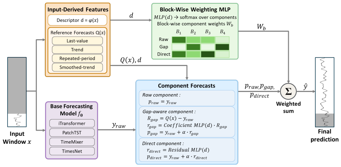
Figure 2.
Block-wise soft weighting in GARS. Component forecasts are combined with block-specific soft weights to form the final prediction.
Figure 2.
Block-wise soft weighting in GARS. Component forecasts are combined with block-specific soft weights to form the final prediction.
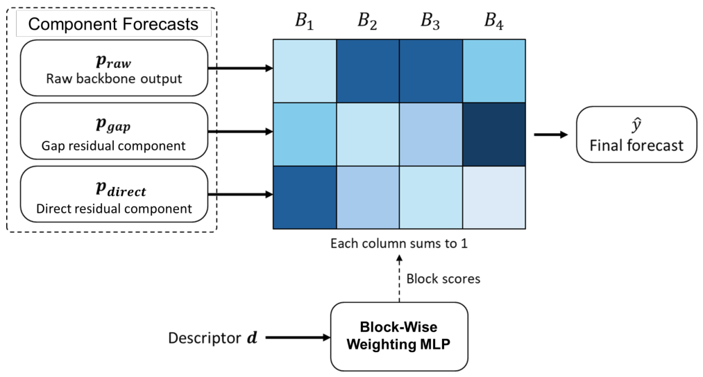
Figure 3.
Relative MSE improvement of GARS over the original model across the 80 main evaluation settings; each point is one dataset–horizon–base-model combination, and positive values indicate a lower MSE than the original model.
Figure 3.
Relative MSE improvement of GARS over the original model across the 80 main evaluation settings; each point is one dataset–horizon–base-model combination, and positive values indicate a lower MSE than the original model.
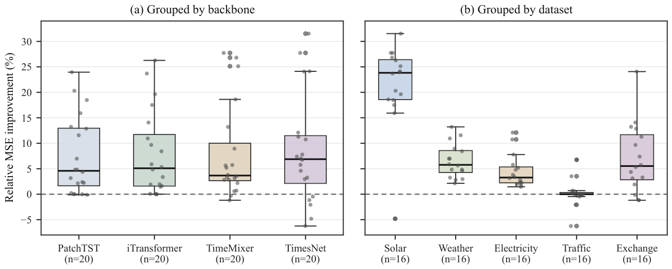

Table 1.
GARS module configuration.
| Module | Configuration |
|---|---|
| Gap coefficient MLP |
Input: descriptor . Architecture: . Activation: GELU after the hidden layer. Output: bounded coefficients after tanh. |
| Direct residual MLP |
Input: descriptor . Architecture: . Activation: GELU after the hidden layer. Output: reshaped to . |
| Block-wise weighting MLP |
Input: descriptor . Architecture: . Activation: GELU after the hidden layer. Output: block-wise component weights. |
GELU, Gaussian error linear unit.
Table 2.
Shared training settings.
| Item | Setting |
|---|---|
| Objective | MSE between and |
| Optimizer | AdamW |
| Initial learning rate | |
| Gradient clipping | |
| Trainable parameters | Base model and GARS parameters are trained jointly |
| Frozen parameters | None |
| Auxiliary losses | None |
| Residual damping | |
| Checkpoint selection | Best validation-MSE checkpoint |
Table 3.
Application-oriented forecasting benchmarks.
| Dataset | Sampling interval | Length | Variables | Description |
|---|---|---|---|---|
| Solar | 10 min | 52,560 | 137 | solar power production records from photovoltaic plants |
| Weather | 10 min | 52,696 | 21 | meteorological measurements collected throughout 2020 |
| Electricity | 1 hour | 26,304 | 321 | electricity consumption records from multiple clients |
| Traffic | 1 hour | 17,544 | 862 | road occupancy rates measured by freeway sensors |
| Exchange | 1 day | 7,588 | 8 | daily exchange rates from multiple countries |
Table 4.
All forecasting experiment results on the application-oriented benchmark datasets.
| Model | iTransformer [15] | PatchTST [14] | TimeMixer [20] | TimesNet [24] | |||||||||||||
|---|---|---|---|---|---|---|---|---|---|---|---|---|---|---|---|---|---|
| Method | Original | GARS | Original | GARS | Original | GARS | Original | GARS | |||||||||
| Metric | MSE | MAE | MSE | MAE | MSE | MAE | MSE | MAE | MSE | MAE | MSE | MAE | MSE | MAE | MSE | MAE | |
| Solar | 96 | 0.280 | 0.313 | 0.231 | 0.301 | 0.269 | 0.302 | 0.226 | 0.292 | 0.282 | 0.312 | 0.229 | 0.300 | 0.297 | 0.315 | 0.225 | 0.304 |
| 192 | 0.325 | 0.340 | 0.261 | 0.328 | 0.318 | 0.330 | 0.260 | 0.324 | 0.340 | 0.346 | 0.254 | 0.319 | 0.346 | 0.344 | 0.237 | 0.307 | |
| 336 | 0.357 | 0.356 | 0.273 | 0.341 | 0.345 | 0.341 | 0.262 | 0.331 | 0.369 | 0.355 | 0.270 | 0.334 | 0.361 | 0.350 | 0.261 | 0.333 | |
| 720 | 0.376 | 0.364 | 0.278 | 0.342 | 0.354 | 0.346 | 0.282 | 0.342 | 0.386 | 0.362 | 0.279 | 0.343 | 0.392 | 0.377 | 0.411 | 0.440 | |
| Avg | 0.334 | 0.343 | 0.260 | 0.328 | 0.322 | 0.330 | 0.258 | 0.322 | 0.344 | 0.344 | 0.258 | 0.324 | 0.349 | 0.346 | 0.284 | 0.346 | |
| Weather | 96 | 0.199 | 0.236 | 0.177 | 0.235 | 0.200 | 0.237 | 0.177 | 0.235 | 0.206 | 0.240 | 0.179 | 0.237 | 0.178 | 0.227 | 0.173 | 0.237 |
| 192 | 0.242 | 0.273 | 0.222 | 0.277 | 0.243 | 0.272 | 0.226 | 0.283 | 0.249 | 0.276 | 0.227 | 0.283 | 0.240 | 0.277 | 0.224 | 0.282 | |
| 336 | 0.262 | 0.296 | 0.249 | 0.312 | 0.258 | 0.293 | 0.252 | 0.318 | 0.262 | 0.296 | 0.255 | 0.319 | 0.255 | 0.294 | 0.246 | 0.317 | |
| 720 | 0.338 | 0.344 | 0.318 | 0.370 | 0.332 | 0.339 | 0.316 | 0.368 | 0.337 | 0.342 | 0.318 | 0.367 | 0.332 | 0.344 | 0.316 | 0.360 | |
| Avg | 0.260 | 0.287 | 0.241 | 0.298 | 0.258 | 0.286 | 0.243 | 0.301 | 0.264 | 0.289 | 0.245 | 0.302 | 0.251 | 0.286 | 0.240 | 0.299 | |
| Electricity | 96 | 0.187 | 0.274 | 0.181 | 0.275 | 0.199 | 0.283 | 0.190 | 0.281 | 0.216 | 0.301 | 0.205 | 0.296 | 0.252 | 0.333 | 0.221 | 0.315 |
| 192 | 0.190 | 0.284 | 0.186 | 0.285 | 0.197 | 0.288 | 0.190 | 0.288 | 0.210 | 0.305 | 0.202 | 0.301 | 0.249 | 0.339 | 0.222 | 0.324 | |
| 336 | 0.213 | 0.304 | 0.210 | 0.305 | 0.215 | 0.305 | 0.210 | 0.304 | 0.229 | 0.321 | 0.223 | 0.318 | 0.262 | 0.350 | 0.247 | 0.340 | |
| 720 | 0.258 | 0.338 | 0.254 | 0.337 | 0.256 | 0.335 | 0.250 | 0.332 | 0.270 | 0.349 | 0.264 | 0.347 | 0.303 | 0.380 | 0.279 | 0.362 | |
| Avg | 0.212 | 0.300 | 0.208 | 0.300 | 0.217 | 0.303 | 0.210 | 0.301 | 0.231 | 0.319 | 0.223 | 0.316 | 0.266 | 0.350 | 0.242 | 0.335 | |
| Traffic | 96 | 0.492 | 0.345 | 0.492 | 0.345 | 0.611 | 0.384 | 0.609 | 0.384 | 0.686 | 0.413 | 0.662 | 0.411 | 0.658 | 0.359 | 0.672 | 0.368 |
| 192 | 0.495 | 0.344 | 0.495 | 0.344 | 0.578 | 0.365 | 0.578 | 0.365 | 0.624 | 0.390 | 0.619 | 0.390 | 0.686 | 0.375 | 0.729 | 0.396 | |
| 336 | 0.520 | 0.357 | 0.520 | 0.357 | 0.587 | 0.369 | 0.587 | 0.369 | 0.632 | 0.395 | 0.628 | 0.395 | 0.722 | 0.394 | 0.673 | 0.368 | |
| 720 | 0.642 | 0.428 | 0.642 | 0.428 | 0.677 | 0.421 | 0.677 | 0.421 | 0.885 | 0.515 | 0.887 | 0.517 | 0.753 | 0.406 | 0.756 | 0.403 | |
| Avg | 0.537 | 0.369 | 0.537 | 0.369 | 0.613 | 0.385 | 0.613 | 0.385 | 0.707 | 0.428 | 0.699 | 0.428 | 0.705 | 0.384 | 0.707 | 0.384 | |
| Exchange | 96 | 0.097 | 0.218 | 0.095 | 0.222 | 0.092 | 0.209 | 0.088 | 0.211 | 0.087 | 0.203 | 0.084 | 0.209 | 0.118 | 0.246 | 0.090 | 0.218 |
| 192 | 0.187 | 0.310 | 0.177 | 0.303 | 0.188 | 0.305 | 0.188 | 0.310 | 0.184 | 0.302 | 0.186 | 0.309 | 0.216 | 0.335 | 0.192 | 0.316 | |
| 336 | 0.327 | 0.416 | 0.295 | 0.404 | 0.345 | 0.425 | 0.301 | 0.404 | 0.325 | 0.412 | 0.314 | 0.411 | 0.400 | 0.462 | 0.371 | 0.443 | |
| 720 | 0.863 | 0.703 | 0.742 | 0.654 | 0.966 | 0.739 | 0.838 | 0.693 | 0.876 | 0.707 | 0.826 | 0.688 | 1.019 | 0.771 | 1.031 | 0.777 | |
| Avg | 0.369 | 0.412 | 0.327 | 0.396 | 0.398 | 0.419 | 0.354 | 0.404 | 0.368 | 0.406 | 0.353 | 0.404 | 0.438 | 0.454 | 0.421 | 0.439 | |
Table 5.
Paired significance of GARS relative to the original model, by dataset.
| Dataset | n | Mean MSE | p (MSE) | Mean MAE | p (MAE) |
|---|---|---|---|---|---|
| Solar | 16 | ||||
| Weather | 16 | ||||
| Electricity | 16 | ||||
| Traffic | 16 | ||||
| Exchange | 16 | ||||
| All | 80 |
Table 6.
Horizon-wise summary of relative MSE and MAE changes.
| Horizon | MSE | MAE | ||
|---|---|---|---|---|
| Mean | Median | Mean | Median | |
| 96 | ||||
| 192 | ||||
| 336 | ||||
| 720 | ||||
Table 7.
Compact component-removal ablation.
| Variant | Components used | Mean MSE | Mean MAE |
|---|---|---|---|
| Full GARS | Initial + gap-aware + direct | ||
| w/o gap-aware | Initial + direct | ||
| w/o direct | Initial + gap-aware |
Table 8.
Setting-level component-removal ablation.
| Dataset | Base model | Horizon | Mean MSE | Mean MAE | ||||
|---|---|---|---|---|---|---|---|---|
| Full | w/o gap-aware | w/o direct | Full | w/o gap-aware | w/o direct | |||
| Electricity | iTransformer | 96 | ||||||
| Electricity | iTransformer | 720 | ||||||
| Electricity | PatchTST | 96 | ||||||
| Electricity | PatchTST | 720 | ||||||
| Electricity | TimeMixer | 96 | ||||||
| Electricity | TimeMixer | 720 | ||||||
| Exchange | iTransformer | 96 | ||||||
| Exchange | iTransformer | 720 | ||||||
| Exchange | PatchTST | 96 | ||||||
| Exchange | PatchTST | 720 | ||||||
| Exchange | TimeMixer | 96 | ||||||
| Exchange | TimeMixer | 720 | ||||||
| Weather | iTransformer | 96 | ||||||
| Weather | iTransformer | 720 | ||||||
| Weather | PatchTST | 96 | ||||||
| Weather | PatchTST | 720 | ||||||
| Weather | TimeMixer | 96 | ||||||
| Weather | TimeMixer | 720 | ||||||
Table 9.
Reference-forecast ablation for the gap-aware residual component.
| Variant | Active forecasts | Mean MSE | Mean MAE | Dataset-wise mean MSE | |||
|---|---|---|---|---|---|---|---|
| Weather | Electricity | Traffic | Exchange | ||||
| Full | V + T + R + S | ||||||
| w/o trend | V + R + S | ||||||
| w/o repeated | V + T + S | ||||||
| w/o last-value | T + R + S | ||||||
| w/o smoothed | V + T + R | ||||||
Table 10.
Residual-scale sensitivity ablation.
| Mean MSE | Median MSE | Mean MAE | |
|---|---|---|---|
| 0.1 | |||
| 0.2 | |||
| 0.3 | |||
| 0.4 | |||
| 0.5 |
Disclaimer/Publisher’s Note: The statements, opinions and data contained in all publications are solely those of the individual author(s) and contributor(s) and not of MDPI and/or the editor(s). MDPI and/or the editor(s) disclaim responsibility for any injury to people or property resulting from any ideas, methods, instructions or products referred to in the content. |
© 2026 by the authors. Licensee MDPI, Basel, Switzerland. This article is an open access article distributed under the terms and conditions of the Creative Commons Attribution (CC BY) license (http://creativecommons.org/licenses/by/4.0/).
Copyright: This open access article is published under a Creative Commons CC BY 4.0 license, which permit the free download, distribution, and reuse, provided that the author and preprint are cited in any reuse.