

Submitted:
29 July 2026
Posted:
30 July 2026
You are already at the latest version
Abstract
Assessing ecological sustainability in agricultural landscapes requires approaches that integrate land-cover change, its ecological effects, and their spatial determinants. This study analysed changes between 2023 and 2024 across 6 agricultural landscapes in northern Benin using the Landscape Ecological Sustainability Index (LESI), calculated for 1-km² landscape cells from Human Disturbance Coefficients (HDCs) assigned to satellite-derived land-cover classes. Spatio-temporal dynamics were assessed using ΔLESI, the Wilcoxon signed-rank test, Global Moran's I, and Local Indicators of Spatial Association (LISA). The contribution of land-cover transitions to HDC change was quantified, and univariate regression models examined the relationships between LESI variations and 11 biophysical and geographical variables. Ecological sustainability declined in 4 sites, improved slightly in one, and remained relatively stable in another. Significant spatial autocorrelation was detected in all sites (Moran's I = 0.44–0.65; p < 0.001). Some spatially limited transitions exerted important effects on HDC change. The low explanatory power of the univariate models (R² ≤ 0.081) indicates that no single variable independently explains the observed changes. This integrated framework provides a reproducible approach for assessing, mapping, and prioritising ecological sustainability trajectories from remote sensing data to support evidence-based agricultural landscape planning and sustainable land management.
Keywords:
ecological sustainability trajectories
; agricultural landscapes
; land-cover transitions
; human disturbance coefficient
; earth observation
; spatial autocorrelation
; Benin
; West-Africa
1. Introduction
By 2100, the global population, estimated at 7.7 billion in 2019, is projected to reach approximately 10.9 billion [1]. Low-income countries in sub-Saharan Africa are expected to account for the largest share of this population growth, owing to persistently high fertility rates (averaging around 4.6 children per woman) and an ongoing demographic transition [2]. Population growth is one of the principal drivers of increasing demand for agricultural commodities, which, in turn, intensifies pressure on agrarian systems [3,4]. Indeed, meeting the food requirements of a global population projected to reach 9.7 billion by 2050 is expected to require an increase in agricultural productivity of approximately 110% [5,6].
The imperative to increase agricultural productivity is transforming cropping systems and driving profound changes in agrarian systems across agricultural landscapes in sub-Saharan Africa. One of the defining characteristics of this transformation is the progressive decline in the amount of cultivable land available per agricultural worker as a consequence of population growth. This reduction has led to increasing agricultural land use intensity, characterised by more frequent and intensive cultivation of farmland, often at the expense of its physical, chemical, and biological quality [7,8]. Such intensification is accompanied by a growing dependence on inorganic external inputs, including mineral fertilisers, pesticides, and herbicides, which are used to enhance productivity but simultaneously contribute to soil degradation, environmental contamination, and biodiversity loss [9,10,11]. Moreover, the expansion of monoculture systems, driven by the objective of maximising yields and farm income, increases the vulnerability of agrarian systems to pest outbreaks. This vulnerability is reinforced by the homogenisation of agricultural landscapes and the simplification of crop rotation schemes, both of which favour pest proliferation [12,13]. Finally, when productivity gains become insufficient to meet rising demand, agricultural expansion remains the predominant strategy, resulting in the conversion of natural vegetation and the cultivation of marginal lands [14,15].
Although these transformations have supported increases in agricultural production, they have also generated substantial environmental externalities that undermine the long-term sustainability of agrarian systems across sub-Saharan Africa. These impacts include biodiversity loss and the degradation of natural habitats [16,17], together with the contamination of surface water and groundwater through nutrient leaching, sedimentation, and saline drainage processes [18]. Furthermore, these dynamics impair ecosystem services that are fundamental to the functioning of cropping systems, including pollination, natural pest regulation, and the maintenance of soil fertility, thereby weakening the biological foundations of agricultural production agricole [19,20]. In addition, the intensification of agricultural practices and land-cover change contribute to increased greenhouse gas emissions, reinforcing the negative feedbacks between agriculture and climate change [21].
These challenges underscore the urgent need to reconfigure farming systems towards models capable of reconciling increased agricultural production with environmental conservation, notably by reducing the negative environmental externalities associated with agricultural intensification [22,23]. This need has stimulated the emergence of several conceptual frameworks, among which sustainable intensification has become particularly influential [24,25]. Sustainable intensification is founded on the principle of increasing or maintaining agricultural production without expanding cultivated land or causing net environmental degradation [15].
Achieving these two objectives simultaneously, however, cannot rely on standardised approaches. Agrarian systems exhibit considerable heterogeneity in terms of their biophysical and geographical conditions, cropping systems, and socio-economic contexts. Consequently, understanding the ecological dynamics specific to individual agricultural landscapes is essential for identifying management strategies capable of effectively reconciling agricultural production with environmental conservation in agrarian systems [26].
As in many other tropical regions, the expansion of agricultural land is the primary driver of natural ecosystem degradation [27,28,29] in the agricultural landscapes of northern Benin, located within the Sudanian zone of West Africa. This region alone accounts for approximately 81% of the country's cultivated agricultural land and constitutes Benin's principal agricultural production basin, making a dominant contribution to the national production of crops such as maize, cotton, cashew, and soybean [30]. The increase in agricultural production observed over recent decades has been driven largely by the expansion of cultivated land rather than by substantial gains in agricultural productivity [30]. This process of agricultural expansion has been accompanied by the progressive degradation of ecosystems and the services they provide, notably through soil erosion, sedimentation, water eutrophication, biodiversity loss, and increased greenhouse gas emissions [31,32,33,34]. Moreover, agrarian systems in this region are characterised by an increasing reliance on inorganic inputs, particularly mineral fertilisers, herbicides, and pesticides, which contribute to the degradation of both terrestrial and aquatic ecosystems. Consequently, the agrarian systems of northern Benin provide a particularly relevant case study for investigating the trade-offs between agricultural intensification, farmland expansion, and the ecological sustainability of Sudanian agricultural landscapes.
Research on the ecological sustainability of agricultural landscapes generally focuses on three complementary levels of analysis. The first seeks to characterise the spatio-temporal dynamics of landscape ecological condition using Earth observation-derived indicators, composite indices, or spatial analyses conducted at successive time periods [35,36,37]. The second relates these ecological changes to land-cover dynamics by examining land-cover change and landscape trajectories [38]. The third aims to identify the biophysical and geographical factors driving these dynamics using statistical or machine learning models, thereby explaining the observed spatio-temporal patterns of change [39]. Although these approaches are well established in the literature, they are generally applied independently, limiting a comprehensive understanding of the spatio-temporal dynamics of ecological sustainability in agricultural landscapes and their relationships with land-cover change and the spatial distribution of biophysical and geographical drivers.
Against this background, this chapter addresses the following research questions:
(1) How has the ecological sustainability of agricultural landscapes in northern Benin changed over space and time?
(2) Which land-cover transitions have driven the observed changes in ecological sustainability?
(3) Which biophysical and geographical factors determine the spatio-temporal dynamics of ecological sustainability in the agricultural landscapes of northern Benin?
2. Materials and Methods
2.1. Study Area
The study area is located between 8.45°–11.68° N and 1.35°–3.85° E (Figure 1). It covers 65,926 km², representing approximately 57% of the total land area of Benin, a country situated in West Africa [40]. The six study sites (Bagou, Ouénou, Parakou, Soaodou, Awanla, and Gbanlin) were named after the principal settlements located within each site. They are distributed across four agroecological zones (AEZs) within the northern Benin agricultural basin: the North Cotton Zone (AEZ II), the South Borgou Food Crop Zone (AEZ III), the West Atacora Zone (AEZ IV), and the Central Benin Cotton Zone (AEZ V).
Across these four agroecological zones, the natural vegetation is dominated by wooded savannas characterised by species such as Adansonia digitata, Parkia biglobosa, Vitellaria paradoxa, Ceiba pentandra, and Blighia sapida [41]. The region experiences Sudanian to Sudano-Guinean climatic conditions, with mean annual rainfall ranging from 600 to 1,400 mm. The dominant soil types are ferruginous soils, mainly classified as Lixisols, Leptosols, and Luvisols [42]. The principal crops cultivated in the region include cotton, root and tuber crops, legumes, maize, yam, and cashew [43]. Agricultural production is highly dependent on chemical inputs: 50–71% of farmers apply mineral fertilisers, 70–81% use herbicides, and 51–70% apply insecticides [44].
2.2. Description of Land-Cover Maps
This study is based on a time series of 12-class land-cover maps available for the six study sites for the years 2023 and 2024. These maps were produced by CIRAD as part of the OBSYDYA research project (https://www.obsydya.org/) (Figure 2).
The LULC maps used in this study were generated using the automated Moringa processing chain [45]. This workflow integrates several complementary Earth observation data sources, including very high spatial resolution SPOT 6/7 imagery (1.6 m), Sentinel-2 Level-2A multispectral image time series (10–20 m spatial resolution), and a 30-m Digital Elevation Model (DEM) derived from the Shuttle Radar Topography Mission (SRTM).
The Moringa classification workflow is based on the Random Forest machine learning algorithm implemented through Orfeo ToolBox (OTB) functions, operationalised using Python scripts, and complemented by intermediate processing steps carried out in QGIS. The first stage of the workflow consists of segmenting the very high-resolution imagery to delineate spectrally homogeneous image objects. These objects are subsequently classified using a Random Forest model trained and validated with a reference dataset compiled from field surveys and photo-interpretation.
Field reference data were collected using the QField mobile application installed on tablet devices, initially as georeferenced point observations. These points were subsequently converted into training polygons by digitising the corresponding object boundaries visible on the SPOT 6/7 imagery. Table 1 summarises the classification accuracy metrics obtained for the land-cover maps generated using the Moringa processing chain. Overall classification performance remained high across all study sites for both years, with overall accuracies ranging from 0.79 to 0.90 and Cohen's Kappa coefficients ranging from 0.66 to 0.88. Compared with the 2023 classifications, the 2024 results showed a decline in classification performance across all sites. This decrease was particularly pronounced at Bagou, where overall accuracy declined from 0.90 to 0.82 and the Kappa coefficient from 0.86 to 0.66, and at Soaodou, where overall accuracy decreased from 0.88 to 0.79 and the Kappa coefficient from 0.82 to 0.73.
The minimum size of the features mapped is approximately 20 m², providing the land-cover maps with a high level of spatial detail (Figure 2).
2.3. Unit of Analysis
The spatial unit of analysis adopted for the spatio-temporal assessment of the ecological sustainability of agricultural landscapes in northern Benin was the regular landscape cell [46], defined as a square grid cell of fixed dimensions forming a regular lattice covering the entire study area.
The use of a regular landscape grid offers several methodological advantages. First, it provides a uniform level of cartographic detail, thereby standardising the spatial framework and facilitating the handling of complex geographical information. This approach also avoids the ambiguities associated with reference units of variable size, such as administrative boundaries [47]. Furthermore, regular grids facilitate spatio-temporal comparisons by ensuring that the units of analysis remain constant across both space and time. They provide a common spatial reference framework and enable straightforward aggregation to broader spatial scales without being constrained by administrative divisions [48].
In this study, a 1 km × 1 km landscape cell was selected as the unit of analysis. This spatial resolution represented an appropriate compromise between the level of spatial detail required to capture within-landscape heterogeneity and the computational feasibility of processing the data. It also provided sufficient spatial discrimination to reveal variations in ecological sustainability across the six study sites.
2.4. Temporal Change in the Ecological Sustainability of Agricultural Landscapes
The temporal changes of ecological sustainability were assessed by analysing changes in the Landscape Ecological Sustainability Index (LESI) [49] between the two reference years (2023 and 2024). The Landscape Ecological Sustainability Index (LESI) is an indicator specifically developed to assess the ecological sustainability of agricultural landscapes and is based on the Human Disturbance Coefficient (HDC). The HDC quantifies the intensity of anthropogenic disturbance associated with each land-cover class. It is founded on the principle that different land-cover types exert varying levels of pressure on the major environmental systems, namely the hydrosphere, pedosphere, atmosphere, and biosphere. HDC values range from 1 to 7, with higher values assigned to land-cover classes generating the greatest anthropogenic disturbance and lower values assigned to land-cover types that remain close to their natural condition and exert only limited pressure on ecosystems. The LESI is subsequently calculated as the area-weighted aggregation of the HDC values associated with the different land-cover classes occurring within each landscape cell.
For each landscape cell, the temporal change in ecological sustainability (ΔLESI) was calculated as the difference between the LESI value in 2024 and that in 2023, according to Equation 1.
This equation was used to assign each landscape cell to an ecological sustainability trajectory. Cells exhibiting a decrease in LESI between 2023 and 2024 (ΔLESI < 0) were classified as showing an improvement in ecological sustainability, those with no change (ΔLESI = 0) were considered stable, whereas cells with an increase in LESI (ΔLESI > 0) were classified as undergoing ecological degradation. To facilitate comparison of the magnitude of ecological sustainability changes, ΔLESI values were grouped into five standardised classes applied consistently across the six study sites. A stability threshold ranging from −0.05 to +0.05 was defined to treat minor variations in LESI at the landscape-cell scale as negligible. Values outside this interval were further divided into two levels of change intensity (moderate and high). Accordingly, cells with ΔLESI ≤ −0.20 were classified as exhibiting high improvement, those with values between −0.20 and −0.05 as moderate improvement, values between −0.05 and 0.05 as stable, values between 0.05 and 0.20 as moderate degradation, and those with ΔLESI ≥ 0.20 as high degradation.
For each study site, the proportion of landscape cells associated with improvement, stability, and degradation trajectories was calculated. The median and interquartile range (IQR) of ΔLESI were also computed to summarise, respectively, the central tendency and variability of the observed changes. The distributions of ΔLESI were subsequently visualised using violin plots, enabling comparisons of the magnitude, dispersion, and skewness of ecological sustainability trajectories among the six study sites.
The statistical significance of the observed changes was then assessed using the Wilcoxon signed-rank test, applied to paired LESI values (2023–2024) for each landscape cell. This non-parametric test was selected because of the non-normal distribution of the data and the paired nature of the observations. It assesses whether the median of the paired differences differs significantly from zero, thereby indicating the presence of a significant temporal change in ecological sustainability across the six study sites.
2.5. Spatial Patterns of Changes in the Ecological Sustainability of Agricultural Landscapes
To characterise the spatial dynamics of ecological sustainability, a global spatial autocorrelation analysis was first performed using Moran's Index [50], calculated separately for each study site from the ΔLESI values of the landscape cells. Moran's Index measures the degree of similarity between the ΔLESI value of a given landscape cell and those of its neighbouring cells by comparing the observed spatial covariance with that expected under the assumption of complete spatial randomness. The objective of this analysis was to determine whether the spatial distribution of ΔLESI values exhibited significant spatial organisation, that is, whether geographically proximate cells tended to display similar values or whether the observed pattern was randomly distributed across space.
For each study site, Moran's Index produces a single statistic theoretically ranging from −1 to 1. A value close to 0 indicates the absence of spatial autocorrelation, implying that ΔLESI values are randomly distributed. Conversely, a positive and statistically significant Moran's Index indicates positive spatial autocorrelation, meaning that neighbouring landscape cells tend to exhibit similar ΔLESI values, thereby revealing the presence of spatially homogeneous areas. In contrast, a negative Moran's Index would indicate a checkerboard pattern, characterised by an alternation of contrasting ΔLESI values between adjacent cells.
In a second step, local spatial autocorrelation was investigated using the Local Indicators of Spatial Association (LISA) proposed by Anselin [51]. LISA identifies, for each landscape cell, whether its ΔLESI value is significantly associated with those of its neighbouring cells. The analysis was performed using a first-order Queen contiguity neighbourhood, whereby each landscape cell was considered adjacent to the eight surrounding cells sharing either a side or a corner. The local statistic compares the standardised z-score of ΔLESI value of each landscape cell with the weighted mean of the standardised ΔLESI values observed within its neighbourhood.
The statistical significance of local spatial associations was assessed using a random permutation test. This test involves randomly permuting the ΔLESI values among landscape cells 999 times to generate a reference distribution representing the null hypothesis of no spatial structure. The observed Local Moran's I value is then compared with this simulated distribution to estimate the probability (p-value) that the observed spatial association occurred by chance. Only associations significant at the 5% significance level (p < 0.05) were retained for mapping spatial clusters. Four types of statistically significant spatial configurations were distinguished:
- -
- High–High (HH): a landscape cell with a ΔLESI value above the site mean, surrounded by neighbouring cells that also exhibit above-average ΔLESI values. This configuration represents a cluster of high ΔLESI values, indicating a spatial concentration of areas experiencing relatively low ecological sustainability.
- -
- Low–Low (LL): a landscape cell with a ΔLESI value below the site mean, surrounded by neighbouring cells that also display below-average ΔLESI values. This configuration represents a cluster of low ΔLESI values, identifying areas characterised by relatively higher ecological sustainability.
- -
- High–Low (HL): a landscape cell with an above-average ΔLESI value surrounded by neighbouring cells with below-average values. This pattern represents a positive spatial outlier, indicating a locally more disturbed landscape cell embedded within a relatively more sustainable surrounding landscape.
- -
- Low–High (LH): a landscape cell with a below-average ΔLESI value surrounded by neighbouring cells exhibiting above-average values. This configuration represents a negative spatial outlier, identifying a locally more ecologically sustainable landscape cell within a comparatively less sustainable neighbourhood.
Landscape cells classified as non-significant correspond to situations in which the observed local spatial association did not differ significantly from that expected under a random spatial distribution of ΔLESI values (p ≥ 0.05). Consequently, these cells do not exhibit sufficiently pronounced local spatial structure to be attributed to processes of spatial clustering or spatial contrast.
2.6. Land-Cover Changes Driving the Spatio-Temporal Variation in the Ecological Sustainability of Agricultural Landscapes
To identify the land-cover dynamics underlying the spatio-temporal changes in the ecological sustainability of agricultural landscapes, the adopted approach was based on the analysis of land-cover transition matrices between 2023 and 2024. This approach linked changes in land-cover classes to variations in the Human Disturbance Coefficient (HDC) and, consequently, to changes in LESI.
The analyses were conducted separately for each of the 6 study sites using the land-cover maps produced for 2023 and 2024. For each site, a transition matrix was generated by overlaying the two land-cover maps and comparing the land-cover class assigned to each pixel in 2023 with that in 2024. The resulting matrices therefore quantified both stable land-cover classes and conversions between different land-cover categories. Transition matrices were initially expressed as the number of pixels and subsequently converted into surface areas to quantify the spatial extent of each land-cover transition.
To evaluate the influence of these transitions on ecological sustainability, the transition matrices were subsequently converted into HDC change contribution matrices for each study site. This transformation was based on the HDC values assigned to each land-cover class. For every transition from class i in 2023 to class j in 2024, the contribution to the overall change in the site's HDC was calculated as the product of the proportion of the area affected by the transition and the difference in the HDC values of the two classes (ΔHDC), as expressed in Equation 2:
where:
: represents the contribution of the transition from class i (2023) to class j (2024) to the overall change in the site's HDC;
: is the area that changed from class i in 2023 to class j in 2024;
: is the total area of the study site;
et : are the Human Disturbance Coefficients assigned to the initial and final land-cover classes, respectively.
This equation estimates the specific contribution of each land-cover transition to the overall change in the site's HDC.
The ΔHDC contribution matrices were displayed as matrix tables in which the rows represent the land-cover classes at the initial date and the columns represent those observed at the final date. Each matrix cell indicates the contribution of the corresponding land-cover transition to the overall change in the site's HDC. To facilitate visual interpretation, the contribution values were represented using a colour gradient, with colour intensity proportional to the relative contribution of each land-cover transition to the overall ΔHDC. This contribution depends both on the spatial extent of the transition and on the difference in anthropogenic disturbance between the initial and final land-cover classes. Circle size was scaled according to the area affected by each transition, expressed as a percentage of the total study-site area, thereby distinguishing extensive transitions from more localised ones. This dual representation makes it possible to differentiate the spatial extent of land-cover transitions from their effective contribution to changes in anthropogenic disturbance. Particular attention was paid to identifying the transitions exhibiting the largest positive and negative contributions, thereby distinguishing the principal processes driving the degradation and improvement of ecological sustainability.
2.7. Biophysical and Geographical Factors Driving the Spatio-Temporal Changes in the Ecological Sustainability of Agricultural Landscapes
To investigate the relationships between biophysical and geographical factors and changes in the ecological sustainability of agricultural landscapes, as measured by ΔLESI, the analytical approach focused on examining the functional relationships between each explanatory variable and ΔLESI, without assuming a priori that these relationships were strictly linear.
The analyses were conducted using all 1 km² landscape cells across the six study sites. For each landscape cell, a set of 11 biophysical and geographical variables (Table 2) was extracted and aggregated. Quantitative variables were represented by their mean value within each landscape cell, whereas qualitative variables were represented by their dominant category.
These variables were selected because of their potential influence on both land-cover change and the ecological sustainability of agricultural landscapes. They comprised:
- ▪
- Five soil variables derived from the Soil Property Maps of Africa, produced at a spatial resolution of 250 m [52]:
Depth to bedrock: Depth to bedrock influences several key soil properties, including rooting depth, plant-available water capacity, and nutrient availability. Deep soils generally provide more favourable conditions for agricultural production and are therefore more likely to be converted to cultivation or subjected to agricultural intensification than shallow soils or areas with exposed bedrock. This greater agricultural suitability may promote land-cover change and, consequently, influence the ecological sustainability trajectories of agricultural landscapes. Conversely, shallow soils are generally less suitable for intensive agriculture and are therefore more likely to maintain stable land cover over time.
Soil drainage: Soil drainage describes the ability of soils to remove excess water and therefore directly controls soil moisture conditions. Poorly drained soils, which are prone to frequent or prolonged waterlogging, may constrain agricultural activities and reduce the suitability of land for cultivation. In contrast, moderately to well-drained soils generally provide more favourable conditions for crop development and are consequently more susceptible to agricultural conversion or intensification. Soil drainage may therefore influence land-cover dynamics and, ultimately, the ecological sustainability trajectories of agricultural landscapes.
Soil texture: Soil texture determines water-holding capacity, nutrient availability, permeability, and susceptibility to erosion. Sandy and sandy loam soils, characterised by limited water and nutrient retention, are generally less favourable for intensive agriculture and may therefore restrict certain land-cover conversions. Conversely, silty, clay loam, and clay soils usually possess greater water storage capacity and higher natural fertility, making them more attractive for agricultural production. This increased agricultural suitability may encourage cropland expansion or intensification and consequently influence land-cover change. Soil texture is therefore expected to affect ecological sustainability trajectories indirectly through its influence on the agricultural potential of the land.
Cation exchange capacity (CEC): Cation exchange capacity is a widely recognised indicator of soil fertility and reflects the capacity of soils to retain and supply nutrients to plants. Soils with high CEC values generally provide more favourable conditions for crop production and may therefore be more attractive for agricultural development. This attractiveness may promote the expansion or intensification of agricultural land use, with potential implications for land-cover dynamics and the ecological sustainability of agricultural landscapes. Conversely, soils with low CEC are generally less productive and may therefore experience lower pressure for agricultural conversion or intensification.
Soil water-holding capacity: Soil water-holding capacity refers to the amount of water that a soil can retain and make available to plants after gravitational water has drained away. Unlike soil drainage, which describes the capacity of a soil to remove excess water, this variable reflects the volume of water available for plant uptake. Soils with a high water-holding capacity generally provide more favourable conditions for crop growth, particularly during dry periods, thereby increasing their suitability for agricultural production. Conversely, soils with a low water-holding capacity are more susceptible to water stress and may be less suitable for certain crops. Consequently, this variable is expected to influence land-cover change and, indirectly, the ecological sustainability trajectories of agricultural landscapes.
Terrain Ruggedness Index (TRI): This topographic variable was derived from a 30-m Digital Elevation Model (DEM) [53] and describes the topographic heterogeneity of the landscape. Areas with greater terrain ruggedness generally exhibit lower accessibility and greater constraints on agricultural expansion, thereby favouring the persistence of natural vegetation. Conversely, relatively flat landscapes are typically more suitable for agricultural intensification. Terrain ruggedness is therefore expected to influence both land-cover dynamics and the ecological sustainability of agricultural landscapes.
- ▪
- Two climatic variables, comprising:
Precipitation: This variable was obtained through Inverse Distance Weighting (IDW) interpolation of rainfall records collected between 1980 and 2009 from 43 meteorological stations across Benin, producing a continuous precipitation surface at a 10-m spatial resolution. Precipitation is a major determinant of water availability for both agricultural crops and natural ecosystems. It influences vegetation productivity, the regenerative capacity of plant communities, and the suitability of land for rainfed agriculture. In northern Benin, areas receiving higher rainfall are generally more attractive for agricultural expansion or intensification, which may promote land-cover change and alter levels of anthropogenic disturbance. Conversely, higher rainfall may also support the maintenance of vegetation cover and enhance ecosystem resilience. Precipitation is therefore expected to influence the ecological sustainability trajectories of agricultural landscapes.
Aridity: This variable was derived from the Global Aridity Index dataset at a 1-km spatial resolution [54]. Aridity characterises the degree of hydroclimatic stress experienced by ecosystems. Unlike precipitation, which quantifies only water inputs, the aridity index integrates the balance between water availability and atmospheric evaporative demand. More arid areas generally experience greater water deficits, which may constrain vegetation productivity, reduce ecosystem regeneration capacity, and increase land susceptibility to degradation. These hydroclimatic constraints are likely to influence land-cover decisions, agricultural management practices, and, consequently, the ecological sustainability trajectories of agricultural landscapes.
- ▪
- Three geographical variables, comprising:
Distance to urban areas: This variable corresponds to the Euclidean distance between each landscape cell and the main urban areas, characterised by a high concentration of population, economic activities, and infrastructure. Urban areas were delineated using the GRID3 Settlement Extents v3 (2024) dataset produced by the Center for International Earth Science Information Network (CIESIN). Only features classified as "Built-up area" were retained, while the "Village" and "Hamlet" categories were excluded to ensure that only the principal urban centres likely to exert substantial influence on land-cover dynamics were represented. Proximity to urban areas may increase demand for agricultural land, natural resources, and built-up space, thereby promoting land-cover change and land-cover intensification. Conversely, landscapes located farther from major urban centres are generally less exposed to the direct pressures associated with urban expansion and market accessibility. Distance to urban areas is therefore expected to influence the ecological sustainability trajectories of agricultural landscapes through its effects on land-cover change.
Distance to roads: This variable represents the Euclidean distance from each landscape cell to the paved roads constituting the principal transport corridors within the study area. Transport infrastructure improves access to agricultural land, markets, and natural resources, thereby facilitating human mobility and the establishment of economic activities. Agricultural landscapes located in close proximity to roads are generally more exposed to agricultural expansion, land-cover intensification, natural resource exploitation, and infrastructure development. Conversely, more remote areas often benefit from a degree of isolation that may reduce the intensity of anthropogenic transformations. Distance to roads is therefore expected to influence land-cover change and, consequently, the ecological sustainability trajectories of agricultural landscapes.
Distance to water bodies: This variable corresponds to the Euclidean distance between each landscape cell and permanent and seasonal watercourses derived from a 30-m Digital Elevation Model (DEM) [53]. Proximity to water resources may influence ecological sustainability trajectories through several potentially contrasting mechanisms. On the one hand, riparian areas generally benefit from greater water availability, relatively fertile soils, and the persistence of vegetation associated with aquatic ecosystems, all of which can enhance the ecological resilience of agricultural landscapes. On the other hand, these favourable conditions also make such areas particularly attractive for agriculture, livestock production, and other human activities, potentially leading to land-cover intensification, degradation of riparian vegetation, and increased anthropogenic disturbance. Consequently, distance to water bodies is expected to influence land-cover dynamics and, ultimately, the ecological sustainability trajectories of agricultural landscapes.
A series of univariate regression models was fitted to characterise the relationships between ΔLESI and each of the 11 biophysical and geographical variables. For the continuous variables, six alternative functional forms were evaluated: linear, quadratic, cubic, logarithmic, exponential, and power models. For the categorical variables, Ordinary Least Squares (OLS) regression models were fitted after transforming the categorical predictors using one-hot encoding, whereby each category of a qualitative variable is converted into a binary variable taking the value 1 when the category is present and 0 otherwise [55].
The performance of the competing regression models was evaluated using the coefficient of determination (R²), adjusted coefficient of determination (adjusted R²), root mean square error (RMSE), relative root means square error (RRMSE), mean absolute error (MAE), and the Akaike Information Criterion (AIC).
3. Results
3.1. Spatio-Temporal Changes in the Ecological Sustainability of Agricultural Landscapes
The LESI maps reveal changes in the spatial distribution of ecological sustainability between 2023 and 2024 across all six study sites, although the magnitude of these changes varied among landscape cells (Figure 3). Furthermore, the ΔLESI maps show that changes in ecological sustainability affected the majority of landscape cells. These changes were spatially heterogeneous, resulting in a mosaic of cells undergoing degradation (ΔLESI > 0) and improvement (ΔLESI < 0). The predominance of degrading cells in Awanla, Bagou, Ouenou, and Soaodou indicates a widespread increase in LESI and, consequently, an overall decline in ecological sustainability. By contrast, Gbanlin exhibited a higher proportion of improving cells, reflecting an increase in ecological sustainability between 2023 and 2024. Parakou displayed an intermediate pattern, with improving and degrading cells occurring in relatively balanced proportions.
These spatial patterns are corroborated by the descriptive statistics of ΔLESI (Table 3). Median ΔLESI values were positive in Awanla (0.152), Bagou (0.081), Ouénou (0.135), and Soaodou (0.227), indicating an overall trend towards declining ecological sustainability. Soaodou emerged as the most degraded site, exhibiting both the highest median ΔLESI and the largest proportion of degrading cells (91.24%). In contrast, Gbanlin was the only site with a negative median (−0.018), indicating a slight overall improvement in ecological sustainability, with 55.60% of landscape cells showing a decrease in LESI between the two years. Parakou recorded a median ΔLESI close to zero (0.003), reflecting overall stability in ecological sustainability at the site scale despite the coexistence of improving (48.04%) and degrading (51.32%) landscape cells.
Furthermore, the violin plots (Figure 4) reveal marked spatial heterogeneity in ecological sustainability trajectories within each study site. Although the median values indicate the dominant trend, the wide spread of the distributions demonstrates that processes of ecological improvement and degradation coexisted locally across all 6 sites. The distributions are predominantly shifted towards positive ΔLESI values in Awanla, Ouénou, and Soaodou, reflecting the predominance of degradation processes. In contrast, Gbanlin exhibits a slight predominance of negative ΔLESI values, whereas Parakou appears broadly stable, with a median close to zero. Bagou also displays a slightly positive median, indicating a modest overall tendency towards ecological degradation. Ouénou and Soaodou recorded the largest interquartile ranges (IQRs) (0.195 and 0.250, respectively), indicating greater diversity in local ecological sustainability trajectories. By contrast, Bagou exhibited the smallest IQR (0.124), suggesting a more homogeneous pattern of ecological change across the site.
The Wilcoxon signed-rank test (Table 3) confirms the patterns described above. A significant increase in LESI was observed in Awanla, Bagou, Ouenou, and Soaodou (p < 0.01), where the vast majority of landscape cells (85.24%–91.24%) exhibited a decline in ecological sustainability. In contrast, Gbanlin showed a significant improvement (p < 0.01), with a higher proportion of improving cells (55.60%) than degrading cells (42.68%). By comparison, no significant difference was detected in Parakou (p > 0.05), where the proportions of degrading (51.32%) and improving (48.04%) landscape cells remained nearly balanced.
The Global Moran's I results (Table 4) further revealed a positive and highly significant spatial autocorrelation across all study sites (Moran's I = 0.44–0.65; p < 0.001), indicating that the observed changes were not randomly distributed in space. Instead, neighbouring landscape cells tended to exhibit similar ecological sustainability trajectories.
This spatial organisation is further confirmed by the LISA maps (Figure 3), which reveal statistically significant spatial clusters. Low–Low clusters, representing landscape cells with low ΔLESI values surrounded by neighbouring cells exhibiting similarly low values, are particularly prevalent in Gbanlin and Parakou, indicating the presence of localised areas of improving ecological sustainability. Conversely, High–High clusters, characterised by high ΔLESI values and therefore reflecting ecological degradation, are more frequently observed in Awanla, Ouénou, and Soaodou. Transitional clusters (High–Low and Low–High) are comparatively uncommon, suggesting that changes in ecological sustainability are predominantly organised into coherent spatial patterns rather than occurring as isolated events.
Overall, these findings indicate that temporal changes in ecological sustainability between 2023 and 2024 were characterised by an overall trend towards degradation in four of the six study sites, whereas Gbanlin experienced a slight improvement and Parakou remained broadly stable. They further demonstrate that these changes exhibit significant spatial organisation, reflecting the influence of localised landscape processes on the ecological sustainability of agricultural landscapes.
3.2. Land -Cover Changes Driving the Spatio-Temporal Variation in the Ecological Sustainability of Agricultural Landscapes
Figure 5 highlights the land-cover transitions that contributed most to changes in the Human Disturbance Coefficient (ΔHDC) across the six study sites. Positive contributions (red) represent transitions that increase anthropogenic disturbance and therefore contribute to the degradation of ecological sustainability, whereas negative contributions (blue) correspond to transitions that reduce anthropogenic disturbance and consequently promote improvements in ecological sustainability.
Across all study sites, transitions involving the conversion of natural and semi-natural vegetation into agricultural land emerged as the principal drivers of ecological degradation. The largest positive contributions were generally associated with the conversion of shrub savannas (SHS) into cereal crops (CER), tree crop plantations (OTC), or other agricultural land-cover classes. This transition constituted the dominant contributor in Awanla, Bagou, Ouénou, and Soaodou, where it accounted for a substantial proportion of the increase in ΔHDC observed between 2023 and 2024.
Transitions involving tree crop plantations also represented a major driver of agricultural landscape transformation. In Awanla, Ouénou, and Parakou, the conversion of shrub savannas (SHS) to tree crop plantations (OTC) (predominantly teak plantations) ranked among the principal positive contributors to ΔHDC. This pattern reflects the progressive anthropogenic transformation of agricultural landscapes through the expansion of commercial forest plantations.
Conversely, several land-cover transitions contributed to reducing the overall level of anthropogenic disturbance. These negative contributions were primarily associated with the reconversion of cultivated land to more natural or semi-natural vegetation. In Gbanlin, where the overall ΔHDC remained close to zero and an improvement in LESI was observed, several transitions involving the reversion of agricultural land and plantations to shrub savannas (SHS) made substantial negative contributions to the reduction of anthropogenic disturbance. These restorative transitions largely explain why Gbanlin was the only study site to exhibit a clear improvement in ecological sustainability.
The magnitude of these contributions also varied among the study sites. Soaodou recorded the highest ΔHDC (0.257), characterised by a marked predominance of positive contributions associated with agricultural expansion at the expense of shrub savannas. In contrast, Gbanlin exhibited the lowest ΔHDC (0.003), reflecting a near balance between positive and negative contributions. Awanla (ΔHDC = 0.163), Bagou (ΔHDC = 0.111), and Ouénou (ΔHDC = 0.095) occupied an intermediate position, where the conversion of natural and semi-natural vegetation to agricultural land remained more influential than processes of ecological restoration and natural regeneration.
Finally, the analysis of the contributions of land-cover transitions to ΔHDC (Figure 6) shows that the differences observed among the study sites were driven primarily by a limited number of dominant transitions. In Awanla, the conversion of shrub savanna to cereal crops (SHS → CER) accounted for only 7.8% of the site's total area but alone explained 36.0% of the overall ΔHDC dynamics. Similarly, the transition OTC → CER occupied 9.8% of the site while contributing 20.6% of the total ΔHDC dynamics.
A similar pattern was observed in the other study sites. In Bagou, the transition SHS → CER covered only 5.0% of the landscape yet accounted for 31.4% of the site's overall ΔHDC dynamics. In Ouénou, the transitions OTC → CER and LEG → CER occupied 7.7% and 11.0% of the site, respectively, while contributing 24.0% and 20.6% of the total ΔHDC dynamics. Soaodou, which recorded the highest ΔHDC (0.257), provides the most striking example: although the conversion SHS → CER affected only 15.0% of the site's area, it alone explained 57.4% of the site's ΔHDC, highlighting its pivotal role in the observed ecological degradation.
Conversely, the largest contributions to improving ecological sustainability were associated with transitions towards semi-natural vegetation. In Gbanlin, the transitions OTC → SHS, LEG → SHS, and FTC → SHS occupied 4.2%, 2.3%, and 1.6% of the landscape, respectively, but accounted for 17.7%, 13.0%, and 6.9% of the site's ΔHDC. These restorative transitions almost entirely offset the degradation processes occurring within the site, thereby explaining both its very low ΔHDC (0.003) and the overall improvement in LESI.
Overall, these findings demonstrate that changes in the ecological sustainability of agricultural landscapes depend on both the nature of land-cover transitions and their spatial extent. Relatively limited transitions can exert a major influence on ΔHDC dynamics when they involve substantial changes in anthropogenic disturbance, whereas more extensive transitions may contribute comparatively little to the overall evolution of landscape ecological sustainability.
3.3. Biophysical and Geographical Factors Driving the Spatio-Temporal Changes in the Ecological Sustainability of Agricultural Landscapes
Table 5 presents the best-fitting univariate regression models describing the individual relationships between ΔLESI and the biophysical and geographical variables. Overall, the best-performing models exhibited limited explanatory power, with R² values ranging from 0.0004 to 0.0814. Depth to bedrock (BDRICM) yielded the highest coefficient of determination (R² = 0.0814; p < 0.001), followed by distance to urban areas (DURB; R² = 0.0785; p < 0.001), cation exchange capacity (CEC; R² = 0.0752; p < 0.001), and the Terrain Ruggedness Index (TRI; R² = 0.0586; p < 0.001).
These results indicate that no individual biophysical or geographical variable explains a substantial proportion of the observed variation in the ecological sustainability of agricultural landscapes. Moreover, the predominance of cubic models among the best-fitting regressions suggests that the relationships between ΔLESI and the biophysical and geographical variables are predominantly non-linear.
Figure 7 illustrates the best-fitting univariate relationships between ΔLESI and the biophysical and geographical variables. The fitted regression curves reveal predominantly non-linear relationships. The categorical variables likewise exhibit only modest differences among their respective classes. Specifically, the Humid climatic zone displays slightly higher median ΔLESI values than the Dry sub-humid and Semi-arid zones, whereas differences among soil drainage classes remain limited, despite a slight tendency for poorly drained soils (Low) to be associated with higher ΔLESI values. Similarly, soil texture (TEXMHT) shows virtually no variation among its categories, consistent with the absence of a statistically significant relationship identified in the univariate analyses.
Overall, the scatterplots reveal a substantial dispersion of landscape cells around the fitted regression curves, indicating considerable variability in ΔLESI and confirming that the individual relationships between each explanatory variable and ΔLESI remain weak.
4. Discussion
4.1. Spatial Heterogeneity of Ecological Sustainability Trajectories in Agricultural Landscapes
Among the six study sites, four experienced a decline in ecological sustainability between 2023 and 2024, primarily driven by the expansion of agricultural land-cover classes at the expense of natural vegetation, particularly shrub savannas, and, to a lesser extent, semi-natural formations such as teak plantations. This pattern reinforces the findings of Ahononga, et al. [56] and Biaou, et al. [57], who reported a marked expansion of cultivated land, agricultural fallows, and human settlements in northern Benin between 2005 and 2015. It is also consistent with the broader trend observed across West Africa, where the progressive conversion of natural vegetation into cropland has resulted in declining woody cover and biodiversity [58]. Several studies attribute these changes to evolving agricultural practices, particularly the shortening of fallow periods, population growth, climate variability, and increasing demand for food and energy resources [59]. Declining soil fertility, access to services, and local biophysical conditions have likewise been identified as factors promoting agricultural expansion [60,61,62].
By contrast, Gbanlin was the only study site to exhibit an overall improvement in ecological sustainability, confirming that the trajectories of agricultural landscapes in northern Benin remain spatially heterogeneous [56,57]. This pattern may be partly explained by the presence of Wari-Maro–Mont Kouffé National Park in the western part of the site, which is likely to have constrained agricultural expansion. Indeed, Sassen, et al. [63] showed that protected areas can effectively limit the conversion of natural habitats when conservation measures are properly enforced, although their effectiveness ultimately depends on the institutional capacity to implement and enforce these regulations [64]. Moreover, forest formations within the site were converted to agricultural land to a much lesser extent than shrub savannas. This contrast is consistent with previous studies showing that agricultural expansion generally targets vegetation types that are easier and less costly to clear, particularly savannas, whereas topographic constraints, clearing costs, and certain physical characteristics of the land may limit the conversion of forested areas [65]. In other contexts, however, prior forest degradation, for example through charcoal production, may facilitate their subsequent conversion to agricultural land [66].
Finally, the Global Moran's I and LISA analyses indicate that degrading landscape cells are predominantly organised into spatial clusters, revealing a clear spatial dependence in land transformation processes. This finding is consistent with the work of Mitsuda and Ito [67], who demonstrated that land-cover changes tend to spread to neighbouring parcels. Several authors attribute this pattern to spillover effects, whereby existing agricultural land promotes the expansion of land conversion into adjacent areas, and to the agricultural frontier mechanism, in which land clearing progresses contiguously under the influence of factors such as accessibility, infrastructure, land tenure, and proximity to already cultivated areas [68]. These mechanisms provide a plausible explanation for the spatial organisation of the degradation hotspots identified in the present study.
4.2. Land-Cover Transitions Driving Changes in Ecological Sustainability
The results indicate that the conversion of shrub savannas to cereal crops was the most widespread land-cover transition across the majority of the study sites, making it the principal driver of changes in ecological sustainability. This finding is consistent with the recent evolution of agricultural systems in northern Benin, where landscapes formerly dominated by cotton cultivation have undergone a gradual shift towards food and cash crops, particularly cereals and tubers, in response to market opportunities in southern Benin and neighbouring border regions [69]. This transition has been accompanied by an expansion of cultivated land at the expense of savannas and forest formations [69].
Furthermore, this pattern reflects the functioning of the post-forest agrarian systems described by Mazoyer and Roudart [70]. In these systems, shrub savannas often correspond to medium-term fallows (4–7 years) that are periodically brought back into cultivation to produce short-cycle food crops, particularly cereals. The observed transitions between shrub savannas and cultivated land therefore reflect a farming system based on the alternation of fallow and cultivation phases. However, increasing food demand, coupled with the progressive shortening of fallow periods, may intensify these cultivation cycles, thereby reducing the regenerative capacity of semi-natural vegetation and contributing to the gradual decline in the ecological sustainability of agricultural landscapes.
Finally, the results demonstrate that the ecological significance of a land-cover transition depends not only on its spatial extent but also on the nature of the land-cover classes involved. Consequently, transitions affecting relatively small areas may make a substantial contribution to changes in a site's ΔHDC when they involve marked differences in anthropogenic disturbance between the initial and final land-cover classes. Conversely, more extensive transitions may have a comparatively limited ecological effect because they involve smaller contrasts in disturbance levels. This observation is consistent with the findings of Padonou, et al. [49], who showed that land-cover classes are subject to different levels of anthropogenic pressure and therefore differ in their ecological intensity. These findings highlight the value of complementing conventional land-cover change analyses, which are generally based solely on the extent of converted areas, with approaches that also account for the ecological intensity of land-cover transitions. Such an approach provides a more robust basis for prioritising landscape transformation processes and identifying the transitions with the greatest implications for ecological sustainability.
4.3. Biophysical and Geographical Determinants of Ecological Sustainability Change
The univariate analyses showed that no individual biophysical or geographical variable explained a substantial proportion of the observed variation in ΔLESI. Moreover, the predominance of cubic models among the best-fitting regressions indicates that the relationships between these variables and changes in ecological sustainability are generally non-linear. These findings suggest that ecological sustainability trajectories do not result from the influence of a single driving factor.
This interpretation is consistent with the work of Marshall [71] and Vasseur, et al. [72], who demonstrated that landscape biophysical characteristics, including geomorphology, topography, soil fertility, climate, and drainage, generate environmental gradients that shape the spatial organisation of agroecosystems. These gradients promote the persistence of a landscape mosaic composed of natural, semi-natural, and agricultural land-cover types, whose structural diversity is a key component of the ecological sustainability of agricultural landscapes. However, this spatial organisation is not determined solely by biophysical constraints. Farmers' decisions regarding crop selection, production systems, and land management practices continuously modify this landscape mosaic and, consequently, influence the level of anthropogenic disturbance associated with different land-cover classes. These decisions are themselves shaped by economic, social, cultural, and institutional factors [73,74,75]. In this context, changes in ecological sustainability most likely arise from the interaction between the biophysical characteristics of the landscape and management decisions that govern changes in the composition and spatial configuration of agricultural landscapes.
Nevertheless, the interpretation of these findings remains subject to the methodological assumptions underlying LESI and to the uncertainties associated with land-cover classification. A detailed discussion of these methodological limitations is provided in Padonou, et al. [49].
5. Conclusions
By combining satellite-derived land-cover maps with ecological sustainability indicators (HDC and LESI), this study demonstrates an overall decline in the ecological sustainability of agricultural landscapes in northern Benin between 2023 and 2024, accompanied by marked spatial heterogeneity both among and within the study sites. The conversion of natural and semi-natural land-cover classes to agricultural land, particularly the transition from shrub savannas to cereal crops, emerged as the principal driver of the observed changes. The findings also show that the ecological significance of a land-cover transition depends on both its nature and its spatial extent. Furthermore, no significant univariate relationship was identified between the biophysical and geographical variables considered and changes in ecological sustainability.
Beyond these findings, this study proposes an innovative, integrated, and readily reproducible methodological framework for assessing ecological sustainability trajectories in agricultural landscapes using Earth observation data. By combining LESI, the analysis of land-cover transition contributions to ΔHDC, Local Indicators of Spatial Association (LISA), and univariate regression modelling, the framework simultaneously characterises sustainability trajectories, the land-cover transitions underpinning them, and the factors likely to influence these dynamics. It therefore extends conventional land-cover change analyses based solely on the extent of converted areas by ranking land-cover transitions according to their effective contribution to anthropogenic disturbance, while providing an operational decision-support tool for the monitoring and sustainable management of agricultural landscapes.
Future research should extend this framework to longer time series, explicitly incorporate socio-economic and institutional drivers, and evaluate its transferability across different agroecological contexts in order to further strengthen its operational relevance.
Author Contributions
Conceptualization, Mikhaïl Padonou, Antoine Denis and Gérard Gouwakinnou; Formal analysis, Mikhaïl Padonou and Antoine Denis; Funding acquisition, Antoine Denis, Yvon-Carmen Hountondji and Bernard Tychon; Investigation, Mikhaïl Padonou; Methodology, Mikhaïl Padonou, Antoine Denis and Gérard Gouwakinnou; Project administration, Antoine Denis, Yvon-Carmen Hountondji, Bernard Tychon and Gérard Gouwakinnou; Software, Mikhaïl Padonou; Supervision, Antoine Denis, Yvon-Carmen Hountondji, Bernard Tychon and Gérard Gouwakinnou; Writing – original draft, Mikhaïl Padonou; Writing – review & editing, Mikhaïl Padonou, Antoine Denis and Gérard Gouwakinnou..
Funding
This research was funded by the project “Observatoire pilote des paysages et des dynamiques agricoles du Bénin (OBSYDYA, https://www.obsydya) funded by European Union through the Programme DESIRA N° FOOD/2020/417-846.
Data Availability Statement
Data supporting the findings of this study, as well as any further inquiries, are available from the corresponding author upon request.
Conflicts of Interest
The authors declare no conflicts of interest.
References
- DeSA, U.N. World Population Prospects: 2019 Revision; New York, NY, USA, 2019.
- Bongaarts, J.; Casterline, J. Fertility transition: is sub-Saharan Africa different? 2013, 38, 153. [CrossRef]
- Jiang, L.; Hardee, K. How do recent population trends matter to climate change? 2011, 30, 287-312. [CrossRef]
- Molotoks, A.; Stehfest, E.; Doelman, J.; Albanito, F.; Fitton, N.; Dawson, T.P.; Smith, P. Global projections of future cropland expansion to 2050 and direct impacts on biodiversity and carbon storage. 2018, 24, 5895-5908. [CrossRef]
- Ray, D.K.; Mueller, N.D.; West, P.C.; Foley, J.A. Yield trends are insufficient to double global crop production by 2050. 2013, 8, e66428. [CrossRef]
- Tilman, D.; Balzer, C.; Hill, J.; Befort, B.L. Global food demand and the sustainable intensification of agriculture. 2011, 108, 20260-20264. [CrossRef]
- Mugizi, F.M.; Matsumoto, T. A curse or a blessing? Population pressure and soil quality in Sub-Saharan Africa: Evidence from rural Uganda. 2021, 179, 106851. [CrossRef]
- Drechsel, P.; Kunze, D.; De Vries, F.P. Soil nutrient depletion and population growth in sub-Saharan Africa: a Malthusian nexus? 2001, 22, 411-423. [CrossRef]
- Kopittke, P.M.; Menzies, N.W.; Wang, P.; McKenna, B.A.; Lombi, E. Soil and the intensification of agriculture for global food security. 2019, 132, 105078. [CrossRef]
- Banerjee, S.; Walder, F.; Büchi, L.; Meyer, M.; Held, A.Y.; Gattinger, A.; Keller, T.; Charles, R.; van der Heijden, M.G. Agricultural intensification reduces microbial network complexity and the abundance of keystone taxa in roots. 2019, 13, 1722-1736. [CrossRef]
- De Vries, F.T.; Thébault, E.; Liiri, M.; Birkhofer, K.; Tsiafouli, M.A.; Bjørnlund, L.; Bracht Jørgensen, H.; Brady, M.V.; Christensen, S.; De Ruiter, P.C. Soil food web properties explain ecosystem services across European land use systems. 2013, 110, 14296-14301. [CrossRef]
- Wetzel, W.C.; Kharouba, H.M.; Robinson, M.; Holyoak, M.; Karban, R. Variability in plant nutrients reduces insect herbivore performance. 2016, 539, 425-427. [CrossRef]
- Li, X.; Panke-Buisse, K.; Yao, X.; Coleman-Derr, D.; Ding, C.; Wang, X.; Ruan, H. Peanut plant growth was altered by monocropping-associated microbial enrichment of rhizosphere microbiome. 2020, 446, 655-669. [CrossRef]
- Bezu, S.; Holden, S. Are rural youth in Ethiopia abandoning agriculture? 2014, 64, 259-272. [CrossRef]
- Godfray, H.C.J.; Beddington, J.R.; Crute, I.R.; Haddad, L.; Lawrence, D.; Muir, J.F.; Pretty, J.; Robinson, S.; Thomas, S.M.; Toulmin, C. Food security: the challenge of feeding 9 billion people. 2010, 327, 812-818. [CrossRef]
- Kehoe, L.; Romero-Muñoz, A.; Polaina, E.; Estes, L.; Kreft, H.; Kuemmerle, T. Biodiversity at risk under future cropland expansion and intensification. 2017, 1, 1129-1135. [CrossRef]
- Brink, A.B.; Eva, H.D. Monitoring 25 years of land cover change dynamics in Africa: A sample based remote sensing approach. 2009, 29, 501-512. [CrossRef]
- Bonsch, M.; Popp, A.; Biewald, A.; Rolinski, S.; Schmitz, C.; Weindl, I.; Stevanovic, M.; Högner, K.; Heinke, J.; Ostberg, S. Environmental flow provision: Implications for agricultural water and land-cover at the global scale. 2015, 30, 113-132. [CrossRef]
- Gill, R.J.; Baldock, K.C.; Brown, M.J.; Cresswell, J.E.; Dicks, L.V.; Fountain, M.T.; Garratt, M.P.; Gough, L.A.; Heard, M.S.; Holland, J.M. Protecting an ecosystem service: approaches to understanding and mitigating threats to wild insect pollinators. In Advances in ecological research; Elsevier: 2016; Volume 54, pp. 135-206.
- Aizen, M.A.; Aguiar, S.; Biesmeijer, J.C.; Garibaldi, L.A.; Inouye, D.W.; Jung, C.; Martins, D.J.; Medel, R.; Morales, C.L.; Ngo, H. Global agricultural productivity is threatened by increasing pollinator dependence without a parallel increase in crop diversification. 2019, 25, 3516-3527. [CrossRef]
- Cohen, J.E. Population and climate change. 2010, 154, 158-182. [CrossRef]
- Rockström, J.; Williams, J.; Daily, G.; Noble, A.; Matthews, N.; Gordon, L.; Wetterstrand, H.; DeClerck, F.; Shah, M.; Steduto, P. Sustainable intensification of agriculture for human prosperity and global sustainability. 2017, 46, 4-17. [CrossRef]
- Goulson, D.; Nicholls, E.; Botías, C.; Rotheray, E.L. Bee declines driven by combined stress from parasites, pesticides, and lack of flowers. 2015, 347, 1255957. [CrossRef]
- Gunton, R.M.; Firbank, L.G.; Inman, A.; Winter, D.M. How scalable is sustainable intensification? 2016, 2, 16065. [CrossRef]
- Pretty, J.N. The sustainable intensification of agriculture. In Proceedings of the Natural resources forum, 1997; pp. 247-256.
- Sandhu, H.; Wratten, S.; Costanza, R.; Pretty, J.; Porter, J.R.; Reganold, J. Significance and value of non-traded ecosystem services on farmland. 2015, 3, e762. [CrossRef]
- Tilman, D.; Fargione, J.; Wolff, B.; D'antonio, C.; Dobson, A.; Howarth, R.; Schindler, D.; Schlesinger, W.H.; Simberloff, D.; Swackhamer, D. Forecasting agriculturally driven global environmental change. 2001, 292, 281-284. [CrossRef]
- Gibbs, H.K.; Ruesch, A.S.; Achard, F.; Clayton, M.K.; Holmgren, P.; Ramankutty, N.; Foley, J.A. Tropical forests were the primary sources of new agricultural land in the 1980s and 1990s. 2010, 107, 16732-16737. [CrossRef]
- Dobrovolski, R.; Diniz-Filho, J.A.F.; Loyola, R.D.; De Marco Junior, P. Agricultural expansion and the fate of global conservation priorities. 2011, 20, 2445-2459. [CrossRef]
- DSA. Evolution de la production végétale par commune de 1995 en 2022. Available online: https://dsa.agriculture.gouv.bj/statistics/vegetale (accessed on 30/03/2023).
- Pellikka, P.K.; Clark, B.J.; Gosa, A.G.; Himberg, N.; Hurskainen, P.; Maeda, E.; Mwang’ombe, J.; Omoro, L.M.; Siljander, M. Agricultural expansion and its consequences in the Taita Hills, Kenya. In Developments in earth surface processes; Elsevier: 2013; Volume 16, pp. 165-179.
- Laurance, W.F.; Sayer, J.; Cassman, K.G. Agricultural expansion and its impacts on tropical nature. 2014, 29, 107-116. [CrossRef]
- DeFries, R.S.; Houghton, R.A.; Hansen, M.C.; Field, C.B.; Skole, D.; Townshend, J. Carbon emissions from tropical deforestation and regrowth based on satellite observations for the 1980s and 1990s. 2002, 99, 14256-14261. [CrossRef]
- Fearnside, P.M. Global warming and tropical land-cover change: greenhouse gas emissions from biomass burning, decomposition and soils in forest conversion, shifting cultivation and secondary vegetation. 2000, 46, 115-158. [CrossRef]
- Song, X.-P.; Hansen, M.C.; Stehman, S.V.; Potapov, P.V.; Tyukavina, A.; Vermote, E.F.; Townshend, J.R. Global land change from 1982 to 2016. 2018, 560, 639-643. [CrossRef]
- Uuemaa, E.; Mander, Ü.; Marja, R. Trends in the use of landscape spatial metrics as landscape indicators: A review. 2013, 28, 100-106. [CrossRef]
- Zhu, Z. Change detection using landsat time series: A review of frequencies, preprocessing, algorithms, and applications. 2017, 130, 370-384. [CrossRef]
- Winkler, K.; Fuchs, R.; Rounsevell, M.; Herold, M. Global land use changes are four times greater than previously estimated. 2021, 12, 2501. [CrossRef]
- Meyfroidt, P.; Chowdhury, R.R.; de Bremond, A.; Ellis, E.C.; Erb, K.-H.; Filatova, T.; Garrett, R.; Grove, J.M.; Heinimann, A.; Kuemmerle, T. Middle-range theories of land system change. 2018, 53, 52-67. [CrossRef]
- IGN, B. Limites des départements du Bénin. 2018.
- Ganglo, J.; Henrix, F. Etat de la Recherche Forestière au Bénin-Bilan et Perspectives. In Proceedings of the XII World Forestly Congress, Québec city, Canada, 09/21-28/2003, 2003.
- Aholoukpè, H.; Amadji, G.; Koussihouèdé, H. Chapitre 5. Stocks de carbone dans les sols des zones agro-écologiques du Bénin. In Carbone des sols en Afrique, T. Chevallier, T. M. Razafimbelo, L. Chapuis-Lardy, Brossard, M., Eds.; IRD Édition: Marseille, 2020; pp. 101-112.
- Chadare, F.J.; Fanou Fogny, N.; Madode, Y.E.; Ayosso, J.O.G.; Honfo, S.H.; Kayodé, F.P.P.; Linnemann, A.R.; Hounhouigan, D.J. Local agro-ecological condition-based food resources to promote infant food security: a case study from Benin. Food Security 2018, 10, 1013-1031. [CrossRef]
- PAPA/INRAB. Caractérisation et évaluation des milieux homogènes des zones agroécologiques du Bénin; CRA-Agonkanmey: Benin, 2017; p. 326.
- Stéphane, D.; Laurence, D.; Raffaele, G.; Valérie, A.; Eloise, R. Land cover maps of Antananarivo (capital of Madagascar) produced by processing multisource satellite imagery and geospatial reference data. Data Br 2020, 31, 105952. [CrossRef]
- Peterseil, J.; Wrbka, T.; Plutzar, C.; Schmitzberger, I.; Kiss, A.; Szerencsits, E.; Reiter, K.; Schneider, W.; Suppan, F.; Beissmann, H. Evaluating the ecological sustainability of Austrian agricultural landscapes—the SINUS approach. 2004, 21, 307-320. [CrossRef]
- Walz, U.; Stein, C. Indicators of hemeroby for the monitoring of landscapes in Germany. J. Nat. Conserv. 2014, 22, 279-289, doi:http://dx.doi.org/10.1016/j.jnc.2014.01.007.
- Wonka, E. Flächenstatistik und Datengrundlagen nach regionalstatistischen Rastereinheiten in Österreich. In Flächennutzungsmonitoring [I]: Konzepte-Indikatoren-Statistik, Meinel, G., Schumacher, U., Eds.; Shaker: Aachen, 2009; pp. 155-175.
- Padonou, M.J.D.D.D.; Denis, A.; Hountondji, Y.-C.H.; Tychon, B.; Gouwakinnou, G.N. Multi-Criteria Assessment of the Environmental Sustainability of Agroecosystems in the North Benin Agricultural Basin Using Satellite Data. 2025, 12, 271. [CrossRef]
- Durbin, J. Tests for serial correlation in regression analysis based on the periodogram of least-squares residuals. 1969, 56, 1-15. [CrossRef]
- Anselin, L. Local indicators of spatial association—LISA. 1995, 27, 93-115. [CrossRef]
- Hengl, T.; Heuvelink, G.B.; Kempen, B.; Leenaars, J.G.; Walsh, M.G.; Shepherd, K.D.; Sila, A.; MacMillan, R.A.; Mendes de Jesus, J.; Tamene, L. Mapping soil properties of Africa at 250 m resolution: Random forests significantly improve current predictions. 2015, 10, e0125814. [CrossRef]
- Farr, T.G.; Rosen, P.A.; Caro, E.; Crippen, R.; Duren, R.; Hensley, S.; Kobrick, M.; Paller, M.; Rodriguez, E.; Roth, L. The shuttle radar topography mission. 2007, 45. [CrossRef]
- Zomer, R.J.; Xu, J.; Trabucco, A. Version 3 of the global aridity index and potential evapotranspiration database. 2022, 9, 409. [CrossRef]
- Okada, S.; Ohzeki, M.; Taguchi, S. Efficient partition of integer optimization problems with one-hot encoding. 2019, 9, 13036. [CrossRef]
- Ahononga, F.C.; Gouwakinnou, G.N.; Biaou, S.S.H.; Biaou, S. Vulnérabilité des terres des écosystèmes du domaine soudanien au Bénin de 1995 à 2015. 2020, 346, 35-50. [CrossRef]
- Biaou, S.; Gouwakinnou, G.N.; Biaou, H.S.S.; Tovihessi, M.S.; Awessou, B.K.; Ahononga, F.C.; Houéto, F.O. Identifying the land use and land cover change drivers: methods and case studies of two forest reserves in Northern Benin. 2022, 24, 9885-9905. [CrossRef]
- Brandt, M.; Rasmussen, K.; Hiernaux, P.; Herrmann, S.; Tucker, C.J.; Tong, X.; Tian, F.; Mertz, O.; Kergoat, L.; Mbow, C. Reduction of tree cover in West African woodlands and promotion in semi-arid farmlands. 2018, 11, 328-333. [CrossRef]
- Assédé, E.S.P.; Azihou, A.F.; Geldenhuys, C.J.; Chirwa, P.W.; Biaou, S.S.H. Sudanian versus Zambezian woodlands of Africa: Composition, ecology, biogeography and use. 2020, 107, 103599. [CrossRef]
- Kebede, Y.; Baudron, F.; Bianchi, F.J.; Tittonell, P. Drivers, farmers’ responses and landscape consequences of smallholder farming systems changes in southern Ethiopia. 2019, 17, 383-400. [CrossRef]
- Badmos, B.K.; Villamor, G.B.; Agodzo, S.K.; Odai, S.N.; Guug, S.S. Examining agricultural land-cover/cover change options in rural Northern Ghana: A participatory scenario exploration exercise approach. 2014, 8, 15-35. [CrossRef]
- Wood, E.; Tappan, G.G.; Hadj, A. Understanding the drivers of agricultural land use change in south-central Senegal. 2004, 59, 565-582. [CrossRef]
- Sassen, M.; Sheil, D.; Giller, K.E.; ter Braak, C.J. Complex contexts and dynamic drivers: Understanding four decades of forest loss and recovery in an East African protected area. 2013, 159, 257-268. [CrossRef]
- Angelsen, A. Agricultural expansion and deforestation: modelling the impact of population, market forces and property rights. 1999, 58, 185-218. [CrossRef]
- Chamberlin, J.; Jayne, T.S.; Headey, D. Scarcity amidst abundance? Reassessing the potential for cropland expansion in Africa. 2014, 48, 51-65. [CrossRef]
- Doggart, N.; Morgan-Brown, T.; Lyimo, E.; Mbilinyi, B.; Meshack, C.K.; Sallu, S.M.; Spracklen, D.V. Agriculture is the main driver of deforestation in Tanzania. 2020, 15, 034028. [CrossRef]
- Mitsuda, Y.; Ito, S. A review of spatial-explicit factors determining spatial distribution of land use/land-cover change. 2011, 7, 117-125. [CrossRef]
- Müller, R.; Müller, D.; Schierhorn, F.; Gerold, G. Spatiotemporal modeling of the expansion of mechanized agriculture in the Bolivian lowland forests. 2011, 31, 631-640. [CrossRef]
- Houessè, R.; Mering, C. La déforestation au Nord Bénin: vers une multiplicité de trajectoires territoriales. 2021, 50, 153-174. [CrossRef]
- Mazoyer, M.; Roudart, L. Histoire des agricultures du monde. Du néolithique à la crise contemporaine; Média Diffusion: 2017.
- Marshall, E. Agricultural landscapes: field margin habitats and their interaction with crop production. 2004, 12, 365-404. [CrossRef]
- Vasseur, C.; Joannon, A.; Aviron, S.; Burel, F.; Meynard, J.-M.; Baudry, J. The cropping systems mosaic: how does the hidden heterogeneity of agricultural landscapes drive arthropod populations? 2013, 166, 3-14. [CrossRef]
- Kleijn, D.; Bommarco, R.; Fijen, T.P.; Garibaldi, L.A.; Potts, S.G.; Van Der Putten, W.H. Ecological intensification: bridging the gap between science and practice. 2019, 34, 154-166. [CrossRef]
- Latawiec, A.E.; Strassburg, B.B.; Silva, D.; Alves-Pinto, H.N.; Feltran-Barbieri, R.; Castro, A.; Iribarrem, A.; Rangel, M.C.; Kalif, K.A.B.; Gardner, T. Improving land management in Brazil: A perspective from producers. 2017, 240, 276-286. [CrossRef]
- Martínez-García, C.G.; Dorward, P.; Rehman, T. Factors influencing adoption of improved grassland management by small-scale dairy farmers in central Mexico and the implications for future research on smallholder adoption in developing countries. 2013, 152, 228-238. [CrossRef]
Figure 1.
Study area (II: North cotton zone; III: South Borgou crop zone; IV: West Atacora zone; V: Central Benin cotton zone).
Figure 1.
Study area (II: North cotton zone; III: South Borgou crop zone; IV: West Atacora zone; V: Central Benin cotton zone).
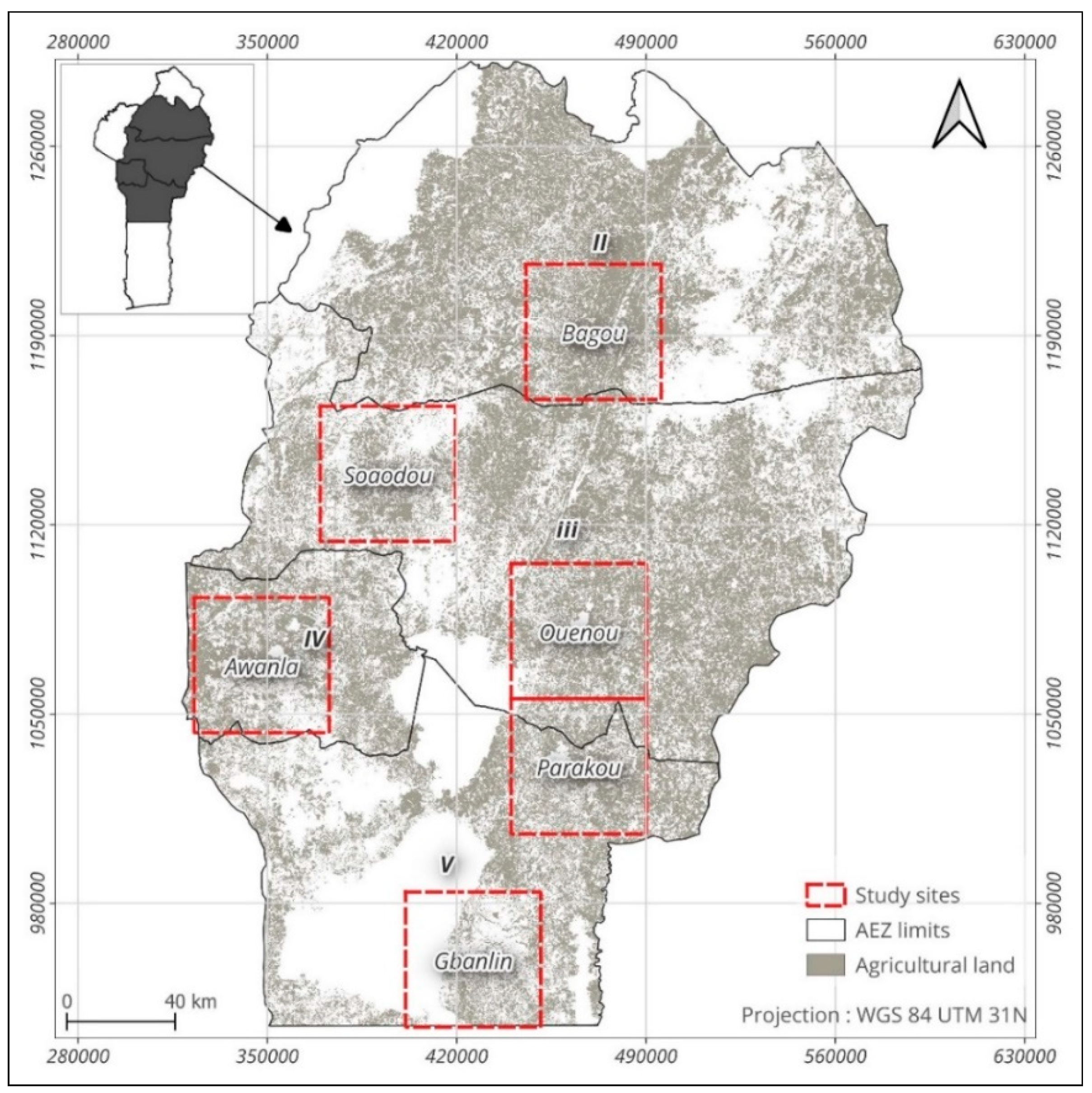
Figure 2.
Types of land cover in the 6 study sites.
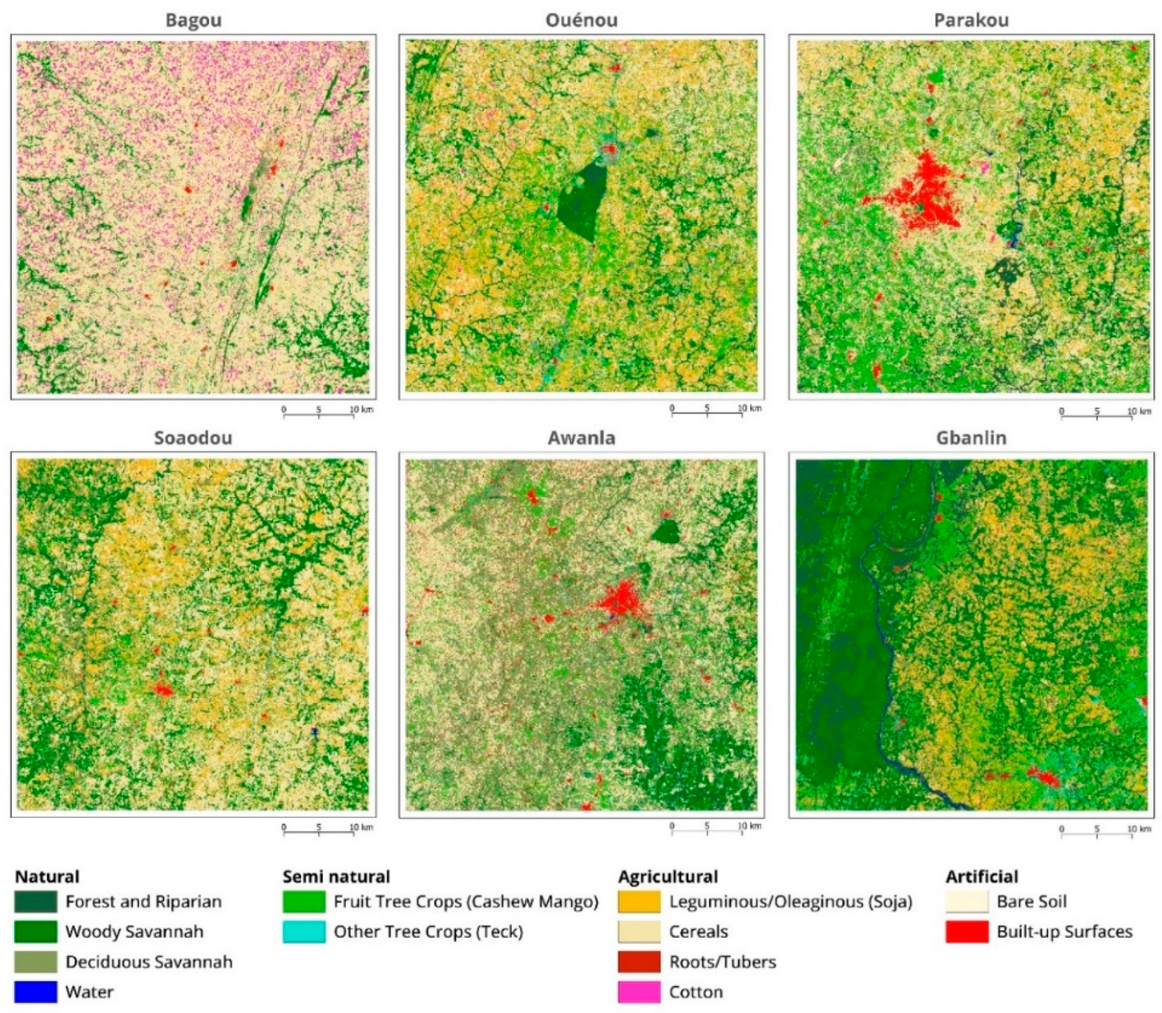
Figure 3.
Spatial distribution of the LESI in 2023 and 2024, year-on-year change (ΔLESI) and Local spatial autocorrelation patterns of the Landscape Ecological Sustainability Index (LESI) across the six study sites.
Figure 3.
Spatial distribution of the LESI in 2023 and 2024, year-on-year change (ΔLESI) and Local spatial autocorrelation patterns of the Landscape Ecological Sustainability Index (LESI) across the six study sites.
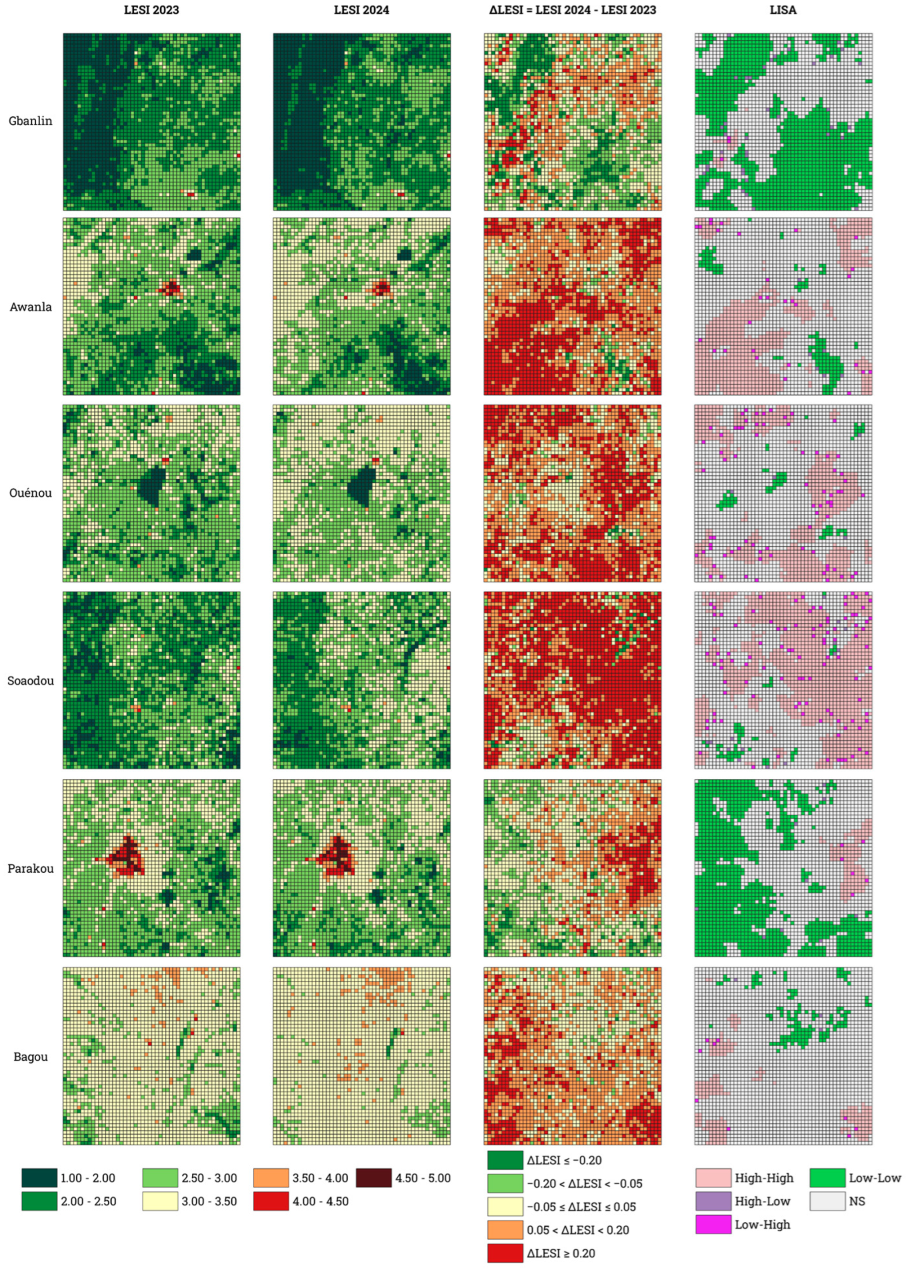
Figure 4.
Violin plots showing the distribution of ΔLESI values across the six study sites between 2023 and 2024. The light-blue violins represent the probability density of ΔLESI values, with wider sections indicating a higher concentration of landscape cells. The horizontal blue bar inside each violin corresponds to the median ΔLESI, while the vertical whiskers indicate the minimum and maximum observed values. The dashed horizontal line represents ΔLESI = 0, separating cells that experienced an improvement (ΔLESI < 0) from those that experienced a degradation (ΔLESI > 0).
Figure 4.
Violin plots showing the distribution of ΔLESI values across the six study sites between 2023 and 2024. The light-blue violins represent the probability density of ΔLESI values, with wider sections indicating a higher concentration of landscape cells. The horizontal blue bar inside each violin corresponds to the median ΔLESI, while the vertical whiskers indicate the minimum and maximum observed values. The dashed horizontal line represents ΔLESI = 0, separating cells that experienced an improvement (ΔLESI < 0) from those that experienced a degradation (ΔLESI > 0).
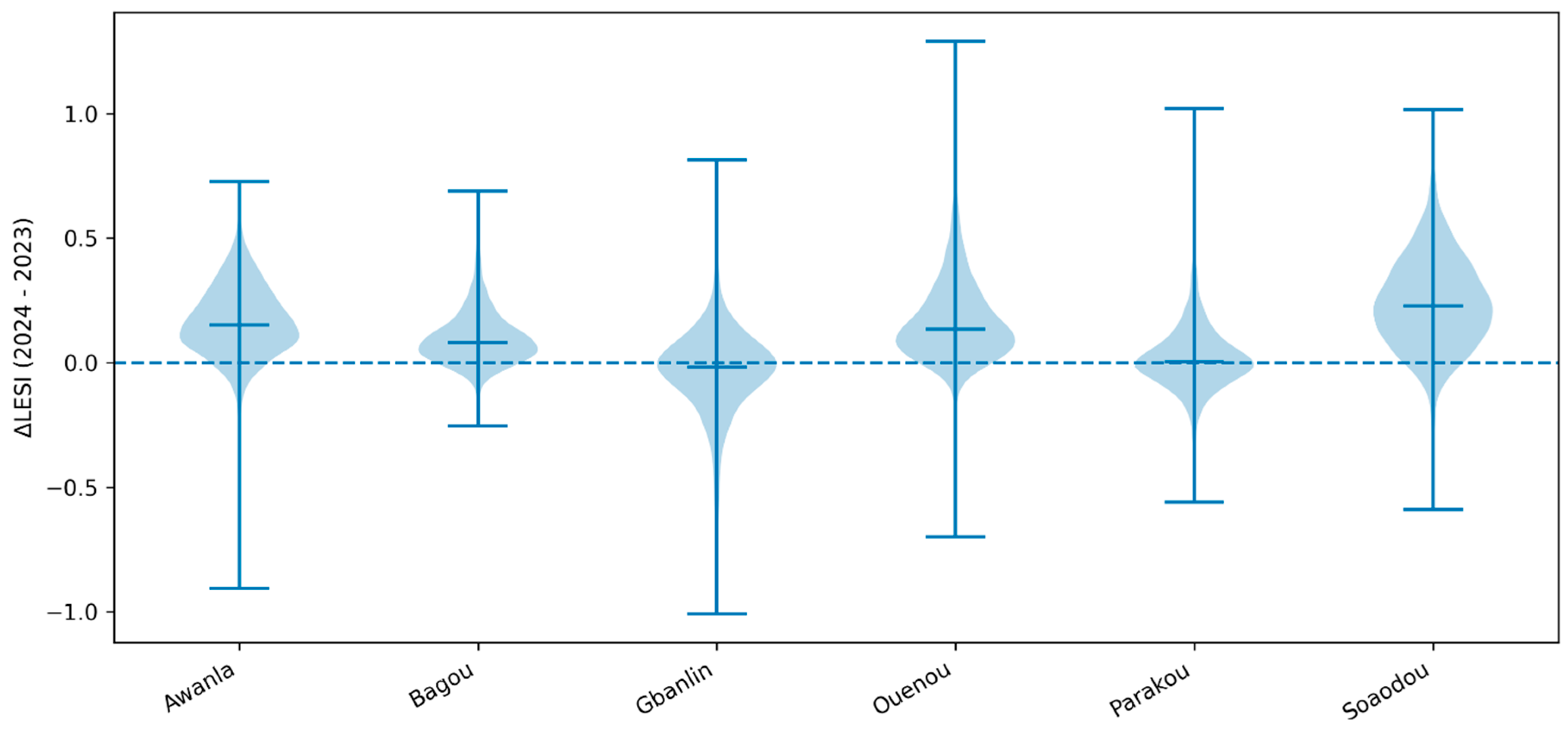
Figure 5.
Absolute contribution of land-cover transitions to changes in the global variation of Human Disturbance Coefficient (ΔHDC) across the six study sites. LEG: Leguminous/Oleaginous (Soja); CER: Cereals; COT: Cotton; RTB: Roots/Tubers; OCR: Other Crops; FTC: Fruit Tree Crops (Cashew, Mango); OTC: Other Tree Crops (Teck); DFO: Dense Forest; OFO: Open Forest; SHS: Shrubby Savannah; BUS: Built-up Surfaces; BAS: Bare Soil; WAT: Water.
Figure 5.
Absolute contribution of land-cover transitions to changes in the global variation of Human Disturbance Coefficient (ΔHDC) across the six study sites. LEG: Leguminous/Oleaginous (Soja); CER: Cereals; COT: Cotton; RTB: Roots/Tubers; OCR: Other Crops; FTC: Fruit Tree Crops (Cashew, Mango); OTC: Other Tree Crops (Teck); DFO: Dense Forest; OFO: Open Forest; SHS: Shrubby Savannah; BUS: Built-up Surfaces; BAS: Bare Soil; WAT: Water.
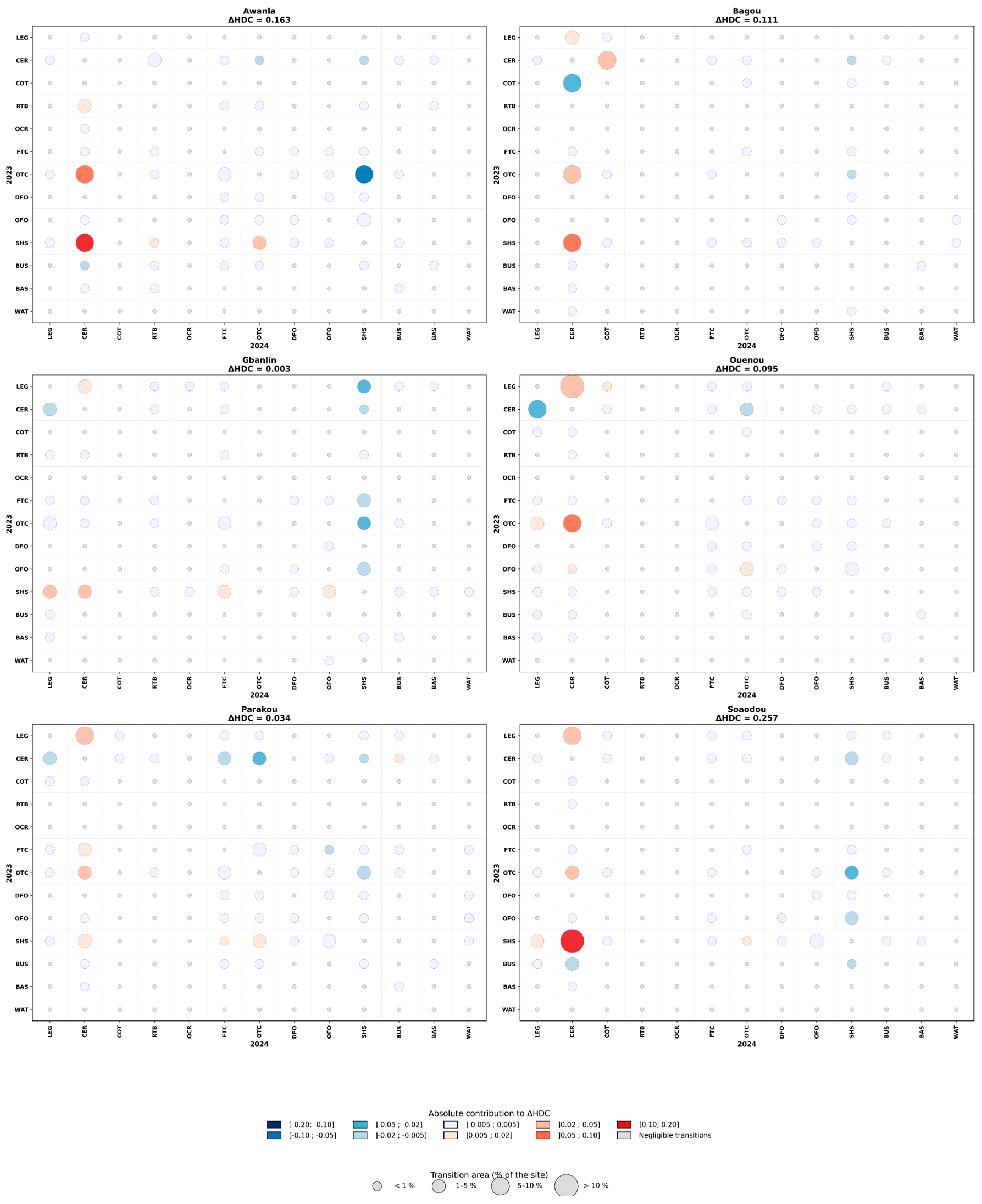
Figure 6.
Main land-cover transitions driving changes in the Human Disturbance Coefficient (ΔHDC) across the six sites between 2023 and 2024. LEG: Leguminous/Oleaginous (Soja); CER: Cereals; COT: Cotton; RTB: Roots/Tubers; OCR: Other Crops; FTC: Fruit Tree Crops (Cashew, Mango); OTC: Other Tree Crops (Teck); DFO: Dense Forest; OFO: Open Forest; SHS: Shrubby Savannah; BUS: Built-up Surfaces; BAS: Bare Soil; WAT: Water. Positive (orange) bars represent land-cover transitions contributing to an increase in anthropogenic disturbance (degradation), whereas negative (green) bars represent transitions contributing to a decrease in disturbance (improvement). Values indicate the absolute contribution of each land-cover transition to the overall change in the Human Disturbance Coefficient (ΔHDC). Values in parentheses correspond to the percentage of the site area occupied by each transition. Only the six most influential transitions are shown for each site.
Figure 6.
Main land-cover transitions driving changes in the Human Disturbance Coefficient (ΔHDC) across the six sites between 2023 and 2024. LEG: Leguminous/Oleaginous (Soja); CER: Cereals; COT: Cotton; RTB: Roots/Tubers; OCR: Other Crops; FTC: Fruit Tree Crops (Cashew, Mango); OTC: Other Tree Crops (Teck); DFO: Dense Forest; OFO: Open Forest; SHS: Shrubby Savannah; BUS: Built-up Surfaces; BAS: Bare Soil; WAT: Water. Positive (orange) bars represent land-cover transitions contributing to an increase in anthropogenic disturbance (degradation), whereas negative (green) bars represent transitions contributing to a decrease in disturbance (improvement). Values indicate the absolute contribution of each land-cover transition to the overall change in the Human Disturbance Coefficient (ΔHDC). Values in parentheses correspond to the percentage of the site area occupied by each transition. Only the six most influential transitions are shown for each site.
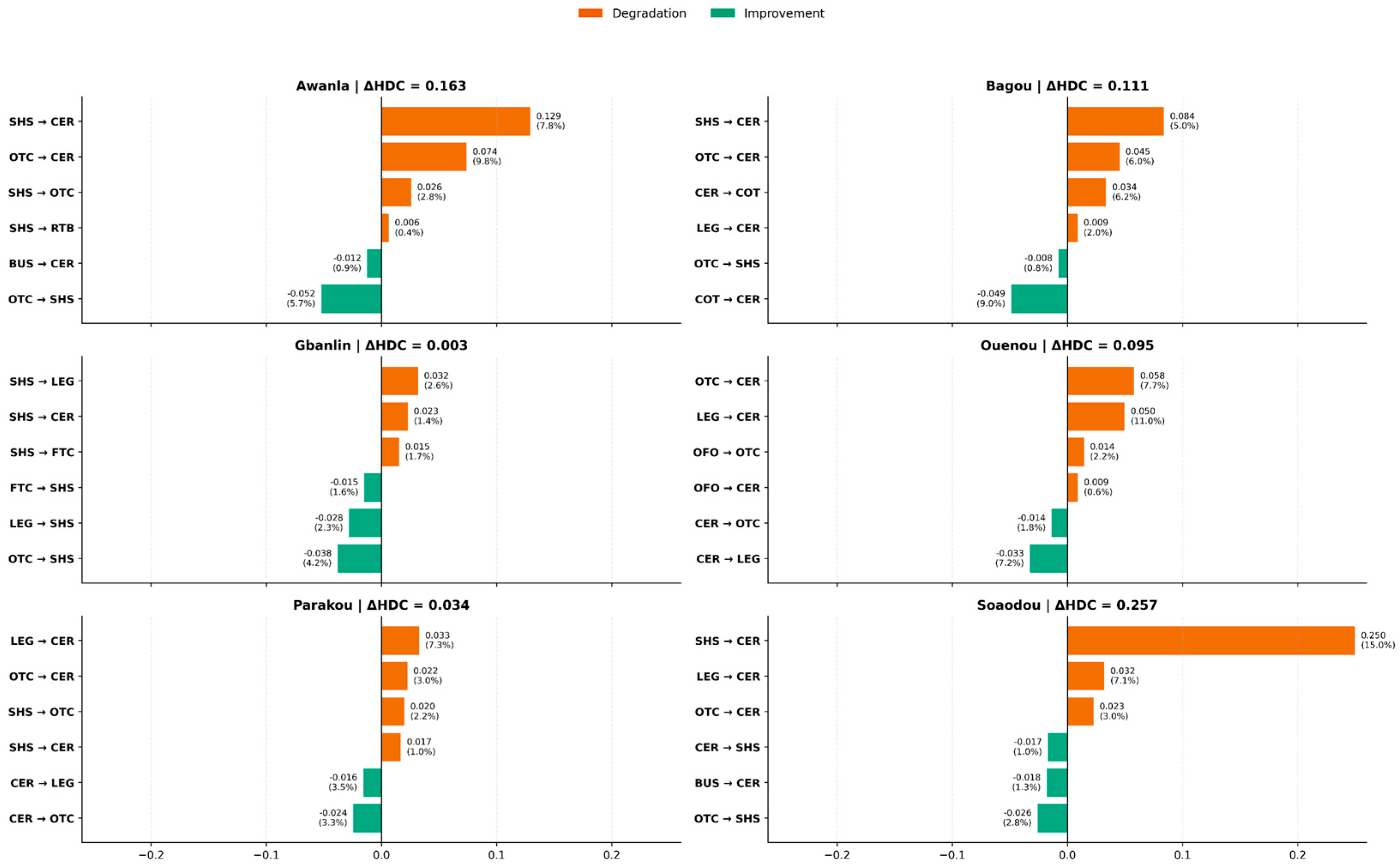
Figure 7.
Best adjusted univariate relationships between ΔLESI and the biophysical and geographical variables. For numerical variables, hexagon shading indicates the density of landscape cells on a logarithmic scale, and the contrasting line represents the best-fitted model. For categorical variables, violins show the distribution density, boxes show the median and interquartile range, and jittered points represent individual landscape cells.
Figure 7.
Best adjusted univariate relationships between ΔLESI and the biophysical and geographical variables. For numerical variables, hexagon shading indicates the density of landscape cells on a logarithmic scale, and the contrasting line represents the best-fitted model. For categorical variables, violins show the distribution density, boxes show the median and interquartile range, and jittered points represent individual landscape cells.
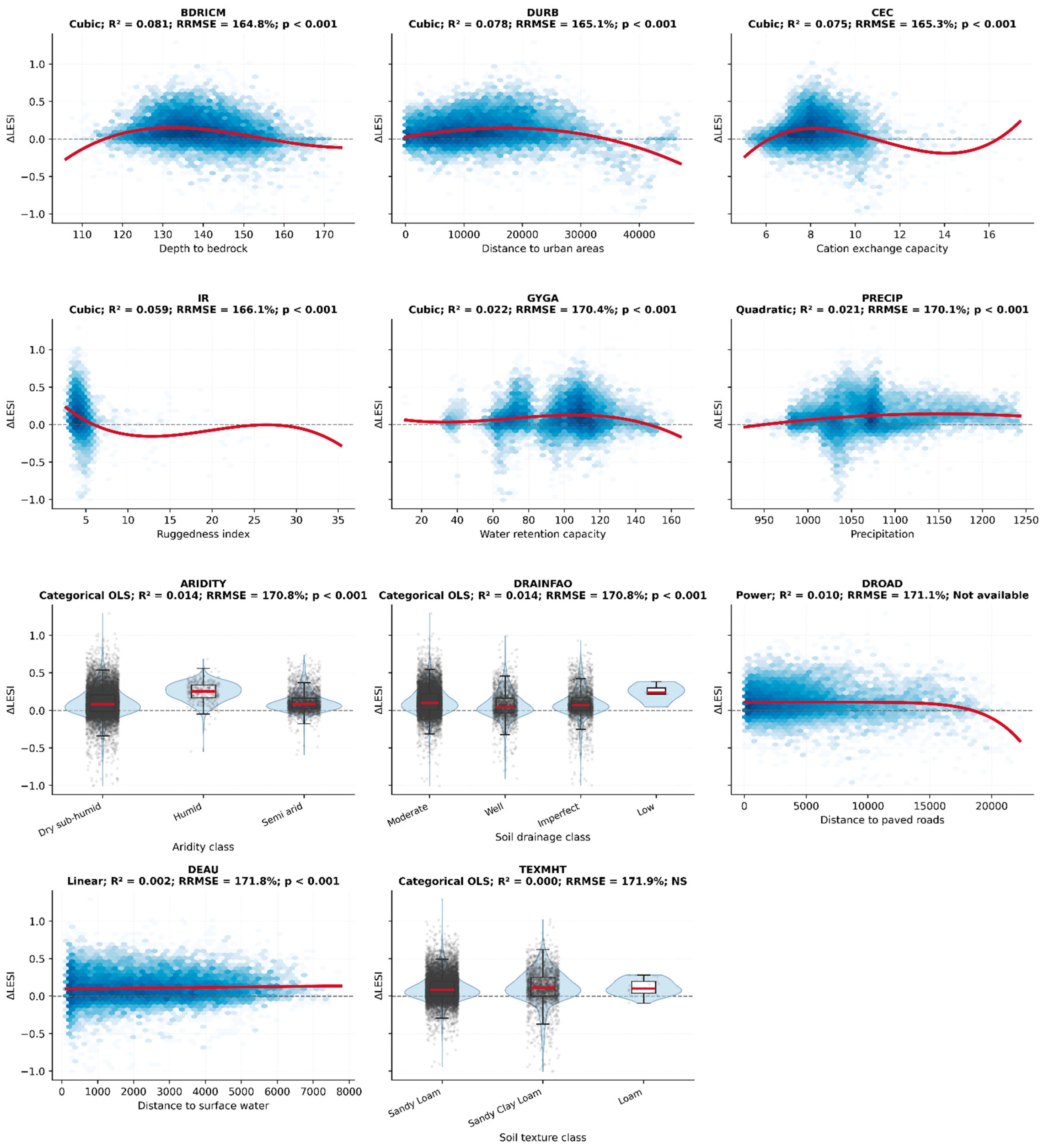

Table 1.
Overall classification accuracy of the land-cover maps.
| Sites | Overall Map Accuracy | Cohen’s Kappa | ||
|---|---|---|---|---|
| 2023 | 2024 | 2023 | 2024 | |
| Bagou | 0.90 ± 0,01 | 0.82 ± 0,02 | 0.86 ± 0,01 | 0.66 ± 0,03 |
| Ouenou | 0.88 ± 0,02 | 0.84 ± 0,01 | 0.84 ± 0,02 | 0.80 ± 0,01 |
| Parakou | 0.86 ± 0,03 | 0.84 ± 0,03 | 0.83 ± 0,04 | 0.81 ± 0,04 |
| Soaodou | 0.88 ± 0,03 | 0.79 ± 0,02 | 0.82 ± 0,04 | 0.73 ± 0,03 |
| Awanla | 0.90 ± 0,02 | 0.84 ± 0,01 | 0.88 ± 0,03 | 0.80 ± 0,01 |
| Gbanli | 0.90 ± 0,02 | 0.88 ± 0,01 | 0.86 ± 0,03 | 0.83 ± 0,01 |
Table 2.
Biophysical and geographical variables aggregated at the landscape-cell level.
| Variable | Code | Category | Unit | Aggregation method | Description |
|---|---|---|---|---|---|
| Depth to bedrock | BDRICM | Biophysical | cm | Mean | Soil depth to bedrock, indicating the volume of soil available for crop root development. |
| Soil drainage | DRAINFAO | Unitless | Dominant class | Soil capacity to remove excess water according to the FAO drainage classification. | |
| Soil texture | TEXMHT | Unitless | Dominant class | Dominant soil texture (clay, sand, or silt), influencing water retention and soil fertility. | |
| Cation exchange capacity | CEC | Cmol (+)/kg | Mean | Soil capacity to retain and exchange essential plant nutrients. | |
| Available water-holding capacity | GYGA | % | Mean | Amount of water available for plant uptake within the soil profile. | |
| Terrain Ruggedness Index | IR | Unitless | Mean | Measure of terrain heterogeneity and topographic complexity. | |
| Precipitation | PRECIP | mm | Mean | Mean annual precipitation. | |
| Aridity | ARIDITY | Unitless | Dominant class | Dominant aridity class. | |
| Distance to urban areas | DURB | Geographical | km | Mean | Distance to major urban centres, used as a proxy for anthropogenic pressure and accessibility. |
| Distance to roads | ROAD | km | Mean | Distance to the principal road network. | |
| Distance to water bodies | DEAU | km | Mean | Distance to surface water resources. |
Table 3.
Wilcoxon signed-rank test.
| Site | ΔLESI Médian | IQR ΔLESI | % ΔLESI>0 | % ΔLESI<0 | % ΔLESI=0 | W | r |
|---|---|---|---|---|---|---|---|
| Awanla | 0,152 | 0,186 | 88,92 % | 10,92 % | 0,16 % | 151 724,0* | 0,782** |
| Bagou | 0,081 | 0,124 | 85,24 % | 14,56 % | 0,20 % | 203 477,0* | 0,753** |
| Gbanlin | -0,018 | 0,177 | 42,68 % | 55,60 % | 1,72 % | 1 201 249,0* | 0,177* |
| Ouenou | 0.135 | 0.195 | 89.24% | 9.00% | 1.76% | 105,278.0* | 0.806** |
| Parakou | 0.003 | 0.133 | 51.32% | 48.04% | 0.64% | 1,396,562.5* | 0.082ns |
| Soaodou | 0.227 | 0.250 | 91.24% | 8.64% | 0.12% | 104,215.0* | 0.808** |
IQR = Interquartile Range; * indicates statistical significance (p-value) at the 1% level for the Wilcoxon signed-rank test, while effect size (r) is interpreted as weak (*), strong (**) or not significant (ns).
Table 4.
Moran’s, I test results.
| Site | n | Moran’s I | p-value | z-score |
|---|---|---|---|---|
| Awanla | 2500 | 0,58 | 0,001 | 59,40 |
| Bagou | 2500 | 0,53 | 0,001 | 51,64 |
| Gbanlin | 2500 | 0,57 | 0,001 | 55,87 |
| Ouenou | 2500 | 0,47 | 0,001 | 45,09 |
| Parakou | 2500 | 0,65 | 0,001 | 61,64 |
| Soaodou | 2500 | 0,44 | 0,001 | 42,12 |
| Global | 15 000 | 0,65 | 0,001 | 154,78 |
Table 5.
Best-fitting univariate regression models describing the relationship between ΔLESI and the biophysical and geographical variables.
Table 5.
Best-fitting univariate regression models describing the relationship between ΔLESI and the biophysical and geographical variables.
| Variable | Model | R² | Adj. R² | RMSE | RRMSE | MAE | p-value |
| BDRICM | Cubic | 0,0814 | 0,08 | 0,18 | 164,81 | 0,13 | p < 0.001 |
| DURB | Cubic | 0,0785 | 0,08 | 0,18 | 165,07 | 0,13 | p < 0.001 |
| CEC | Cubic | 0,0752 | 0,08 | 0,18 | 165,34 | 0,13 | p < 0.001 |
| IR | Cubic | 0,0586 | 0,06 | 0,18 | 166,11 | 0,13 | p < 0.001 |
| GYGA | Cubic | 0,0217 | 0,02 | 0,18 | 170,39 | 0,13 | p < 0.001 |
| PRECIP | Quadratic | 0,0212 | 0,02 | 0,18 | 170,12 | 0,13 | p < 0.001 |
| ARIDITY | OLS | 0,0137 | 0,01 | 0,18 | 170,77 | 0,14 | p < 0.001 |
| DRAINFAO | OLS | 0,0136 | 0,01 | 0,18 | 170,78 | 0,14 | p < 0.001 |
| DROAD | Power | 0,0099 | 0,01 | 0,18 | 171,10 | 0,14 | _ |
| DEAU | Linear | 0,0019 | 0,00 | 0,19 | 171,79 | 0,14 | p < 0.001 |
| TEXMHT | OLS | 0,0004 | 0,00 | 0,19 | 171,92 | 0,14 | NS |
Variable codes: see Table 2. R²: coefficient of determination; Adj. R²: adjusted coefficient of determination; RMSE: root mean square error; RRMSE: relative root means square error; MAE: mean absolute error.
Disclaimer/Publisher’s Note: The statements, opinions and data contained in all publications are solely those of the individual author(s) and contributor(s) and not of MDPI and/or the editor(s). MDPI and/or the editor(s) disclaim responsibility for any injury to people or property resulting from any ideas, methods, instructions or products referred to in the content. |
© 2026 by the authors. Licensee MDPI, Basel, Switzerland. This article is an open access article distributed under the terms and conditions of the Creative Commons Attribution (CC BY) license (http://creativecommons.org/licenses/by/4.0/).
Copyright: This open access article is published under a Creative Commons CC BY 4.0 license, which permit the free download, distribution, and reuse, provided that the author and preprint are cited in any reuse.