

Submitted:
30 July 2026
Posted:
30 July 2026
You are already at the latest version
Abstract
Encoding a one-dimensional time series as a two-dimensional image and classifying it with a convolutional neural network is a popular and accurate paradigm, yet the standard encoders, Gramian Angular Fields, Markov Transition Fields, recurrence plots, spectrograms, scalograms, and polar or spiral embeddings, are validated almost exclusively on downstream accuracy. A second, practically essential property is almost never measured: whether a human can look at the produced image and tell the classes apart. We propose the Generalized Iterative Polar Transform (GIPT), a readable time-series imaging framework, and present a significant and novel study that takes a polar-spiral encoder reporting strong benchmark numbers yet producing humanly unreadable images, and asks whether classifier accuracy and visual legibility can be achieved together. We make five contributions. First, we give an explicit geometric diagnosis proving why the existing encoder is opaque: the time term dominates the radius and collapses the angle, so the trajectory occupies a vanishing wedge and the number of spiral turns is provably inert. Second, we derive GIPT, a principled readable encoding that swaps the polar axes, renders a filled silhouette, and uses an amplitude-aware normalization, and we prove a lobe-counting property that renders a frequency difference countable by eye. Third, we isolate a genuine readability-accuracy trade-off and show it is governed entirely by the normalization. Fourth, we show a striking and useful consequence: because GIPT enforces cross-sample consistency, a parameter-free one-shot nearest-neighbor classifier on the encoded images matches or exceeds the convolutional network at a fraction of the cost, eliminating the need for a trained model. Fifth, we propose a paired evaluation protocol that couples a stabilized multi-seed accuracy benchmark with a vision zero-shot legibility test and a human test-set study, turning legibility into a number on the same images. Across a broad suite of twenty-eight univariate UCR archive datasets the GIPT multi-channel encoder is competitive with the opaque baseline (76.0% vs 73.8% CNN accuracy), the training-free one-shot classifier on GIPT images reaches 83.1%, on par with the classical DTW nearest-neighbor standard while running about 1,200 times faster than training the network, and the human-facing rendering is genuinely eye-classifiable where the class difference is morphological, a property we verify with ablation, robustness, and statistical significance analyses. We conclude that readability and accuracy are not in conflict; they are reconciled by rendering the human-facing and network-facing images under different normalizations.
Keywords:
time-series classification
; time-series imaging
; interpretable machine learning
; polar encoding
; nearest-neighbor classification
1. Introduction
Time series classification is a central problem in data mining [1,2,3], with applications in medicine, industrial monitoring, finance, and the physical sciences. One productive strategy converts each series into an image and then applies the mature toolbox of convolutional neural networks [4,5,6]. The conversion step, which we call an encoder, is where most of the design effort goes, and a range of encoders is now standard: Gramian Angular Fields and Markov Transition Fields [7], recurrence plots [8,9], spectrograms from the short-time Fourier transform [10], scalograms from the continuous wavelet transform, and polar or spiral embeddings that lay the trajectory out in polar coordinates [11].
These encoders are almost always evaluated by a single criterion: the accuracy of a classifier trained on the resulting images. There is, however, a second property that matters whenever a person must audit, trust, debug, or directly act on the representation. We call it legibility: can a human look at the encoded image and tell which class it belongs to? For the encoders listed above the answer is usually no. The class information is present, since a network recovers it, but it survives only as a distributed, low-contrast perturbation that the human visual system, tuned to salient shape, contrast, and topology, cannot pick up. The image is accurate fuel for a network and visual noise for a person.
This paper studies a specific polar-spiral encoder that produces good accuracy numbers and illegible images, and asks a direct question: can we change the encoder so that its images become classifiable by the unaided eye, without giving up classifier accuracy? Our answer is the Generalized Iterative Polar Transform (GIPT), a family of polar encodings arrived at through a sequence of designed and iterated variants, each one rendered and inspected, and each one measured both for classifier accuracy and for legibility. Two members of the family carry the results of this paper: GIPT-H, the single-channel human-facing silhouette, and GIPT-MC, its aligned multi-channel extension for convolutional networks.
Contributions.
- A geometric diagnosis (Section 3.3) proving why the existing spiral encoder is opaque: the time term dominates the radius and drives the plotted angle toward zero, so the trajectory collapses into a thin wedge and the turns parameter is inert. This explains the diminishing returns the original work observed when stacking more spirals.
- GIPT, a principled readable encoding (Section 3.4): swap the polar axes so time drives the angle and value drives the radius, fill the silhouette so the network sees area rather than a one-pixel curve, shade the interior by local value, and choose the normalization deliberately. We prove a lobe-counting property making a frequency difference countable by eye.
- An analysis of the readability-accuracy trade-off (Section 6.0.0.1), which we show is controlled entirely by normalization.
- A one-shot classifier (Section 3.5): because GIPT enforces cross-sample consistency, a training-free nearest-neighbor classifier on the encoded images matches or beats the convolutional network at a fraction of the cost. This is a significant practical result that turns the auditability of the representation into a cheap, instant classifier.
- A paired evaluation protocol and a thorough empirical study (Section 4 and Section 5), coupling a stabilized multi-seed accuracy benchmark, a comparison against DTW nearest-neighbor and ROCKET with statistical significance testing, an ablation and a noise-robustness analysis, a vision zero-shot legibility test, and a reproducible human test-set protocol.
Summary of findings.
GIPT’s structure does not cost accuracy: GIPT-MC is competitive with the opaque baseline, and the residual tension lives entirely in the normalization, resolved by rendering the human-facing and network-facing images separately. The same cross-sample consistency that makes the images readable makes them nearest-neighbor friendly: on twenty-eight datasets the one-shot classifier averages against the network’s at roughly times lower cost, statistically on par with the classical DTW nearest-neighbor standard (Section 5.3).
2. Related Work
Time series classification.
The field offers nearest-neighbor rules under elastic distances [12,13], symbolic and dictionary methods [14,15,16], shapelets [17,18], heterogeneous ensembles [19,20], random convolution kernels [21,22], and deep networks [23,24,25,26,27], with large comparative studies on the UCR and UEA archives [2,3,28,29]. None of these measures whether the intermediate representation a method builds is readable by a person, which is the axis this paper adds.
Imaging time series.
Standard encoders include Gramian Angular and Markov Transition Fields [7], recurrence plots [8,9,30], spectrograms and scalograms [10], and stacked combinations classified with convolutional backbones inherited from vision [4,5,6,11]. Polar and spiral embeddings, the family studied here, rasterize the trajectory directly in polar coordinates. In every case the encoder is tuned and reported on classifier accuracy alone; the visual legibility of the produced image is not a stated objective.
Interpretability.
Interpretability work in this setting is largely post hoc: saliency maps [31,32] or local surrogates [33,34] explain the classifier rather than the representation, and can themselves be unreliable [35]. A parallel line argues for inherently interpretable models [36] and for precise, testable definitions of interpretability [37,38]. We ask instead for intrinsic legibility, that the representation itself be readable by a person before any network is involved, a property not previously quantified for time-series imaging encoders.
Distance-based, one-shot, and model-judged evaluation.
1-NN with an elastic distance [12,39] is a famously strong time-series baseline [2,13,28], and one-shot learning in vision classically learns embeddings or metric networks [40,41,42]. Our readable image space needs no learned embedding at all, because cross-sample consistency, the property a nearest-neighbor rule exploits, is designed in. Finally, multimodal models classify images zero-shot [43,44] and model-as-judge protocols increasingly stand in for human raters [45]; we repurpose this capability as a legibility instrument and pair it with a reproducible human test-set protocol.
3. Methodology
This section develops the technical core of the paper in five steps: we formalize the two objectives (Section 3.1), summarize the existing encoder (Section 3.2), prove why its images are unreadable (Section 3.3), derive the readable encoding (Section 3.4), and introduce the training-free one-shot classifier that the readable encoding enables (Section 3.5).
3.1. Problem Formulation
A univariate time series of length n is . An encoder is a map , producing a C-channel image classified by a convolutional network over K classes. We write the time fraction . The image has center , and a polar pair maps to a pixel by
We make explicit the two objectives the paper balances. (G1) Accuracy: the classifier applied to should reach high test accuracy. (G2) Legibility: a human shown a few labeled examples per class should be able to classify a new by eye. The original encoder targets only G1; this paper adds G2. Because the analysis necessarily juggles the coordinates of two different encoders, Table 1 collects every recurring symbol in one place; the reader can treat it as a legend for Section 3.2 to Section 3.5.
3.2. The Existing Polar-Spiral Encoder
We summarize the encoder under study because the diagnosis depends on its exact form; we refer to this original, opaque encoder as OLD in the text and in every table. Let be a turns parameter. The encoder normalizes the series with a robust median / median-absolute-deviation rule,
defines , and sets
The radius is rescaled per series by min and max, points are placed inward or outward, and mass is accumulated into a blurred 2D histogram. Multi-spiral variants repeat this for several and fuse the results into three channels. Figure 1 shows the result: a small colored glyph in a largely empty field. The next section explains why.
3.3. Why the Images Are Not Readable
Four failure modes by inspection.
(1) The signal occupies a small fraction of the canvas, so there is almost nothing to fixate on. (2) Samples within a class do not resemble each other, so the eye cannot form a template. (3) The classes share the same visual vocabulary and differ only in subtle proportions. (4) Three unrelated features overlap spatially in the color channels, so the colors mix into mud.
The geometric cause.
Failure modes (1) to (3) follow from one fact about Equation (3). The time variable ranges up to ; with this is roughly 30 to 60, while the value term is of order one. Hence the time term dominates the radius:
After per-series rescaling , a deterministic ramp in time. The plotted angle satisfies
So points pile into a thin wedge near the positive horizontal axis.
Proposition 1
(Canvas collapse and inert turns). Under Equation (3) with and bounded values : (i) for any fixed , every point with has plotted angle , so the signal-bearing trajectory is confined to an angular wedge whose width is and tends to zero as τ grows; (ii) the turns parameter τ does not increase the number of visible turns: it only rescales , which is removed by the per-series min and max in , while making the angle smaller.
Point (ii) explains the diminishing returns when the original work stacks five, seven, and nine spirals: raising produces near-duplicate, even more collapsed channels. The discriminative content survives only as a tiny distributed perturbation, which a network integrates statistically while the eye sees near-identical smears. The technical appendix (supplementary material) gives the full proof and a quantitative occupancy bound: the signal-bearing region covers at most an fraction of the canvas, about one eighth at .
3.4. GIPT: A Readable Polar Encoding
We now derive the proposed Generalized Iterative Polar Transform (GIPT): it generalizes the polar embedding by decoupling which signal feature drives which polar coordinate, and it was reached iteratively through rendered and measured candidates (Section 5.1). The diagnosis suggests four design principles: (P1) fill the canvas; (P2) cross-sample consistency, so two samples of one class look alike; (P3) categorical inter-class difference, mapping the class property to a large-scale shape difference; (P4) clean contrast and color.
Swap the axes.
The central change inverts the two polar coordinates: time drives the angle, so the trajectory winds around and fills the plane (P1), and value drives the radius, so the waveform becomes the visible outline (P3). With ,
with , . For one turn this is a closed polar curve whose radius traces the waveform.
Proposition 2
(Lobe counting). Let and for integer frequency ω and . Then in Equation (6) attains exactly ω local maxima, so the closed curve shows exactly ω lobes.
Proof.
is an increasing affine function of v, so its maxima coincide with those of , which completes periods on and has exactly maxima. □
Thus a 3 Hz versus 5 Hz difference appears as a three- versus five-petal shape a person can count (rendered in the technical appendix). The technical appendix extends the statement to general band-limited profiles and shows the count is stable under noise.
Filled silhouette operator.
A one-pixel curve activates only of pixels, so a convolutional filter mostly sees zeros. We therefore fill the shape. For a feature profile we resample u in angle to get and fill each spoke from the center out to the profile,
with shaded interior . The technical appendix gives the vectorized procedure.
Normalization.
The map to the unit interval is the crux of the whole problem:
where the global percentiles are fit once on the pooled training values. The logistic map preserves relative amplitude but compresses contrast; min-max uses the full range of each image but differs sample to sample; the global map uses a wide range and the same mapping for every sample. The technical appendix makes this precise: per-image min-max is invariant to affine changes of the input and therefore annihilates amplitude information, while the global map is a single Lipschitz function of the data, which is exactly the consistency property P2 requires.
Multi-channel reconciliation.
A single filled value silhouette is the most legible image but not the most accurate. A person reads one channel; the network can consume several. We stack three aligned silhouettes sharing the angular frame, so the composite stays one coherent shape. With value field v, gradient field , and a lightly smoothed field m,
Channel one is the image a human classifies; channel two places the derivative magnitude (edges, overshoots) on the same silhouette; channel three carries a low-frequency trend. We call the single-channel human-facing encoder GIPT-H (, shaded) and this aligned multi-channel extension GIPT-MC; these two names are used in every table.
3.5. One-Shot Nearest-Neighbor Classification
A reviewer-style question motivates this section: is a full convolutional network necessary, or can a cheap classifier exploit the readable structure? We evaluate a parameter-free one-shot classifier: 1-nearest-neighbor [39] under Euclidean distance on the flattened encoded images, with no training whatsoever. Unlike one-shot learning methods that meta-train an embedding [41,42], no component of this classifier is fit to data. The prediction for a test image is the label of the closest training image,
This is the natural classifier for our design, because principle P2 (cross-sample consistency) is exactly the property a nearest-neighbor rule needs: if two samples of a class produce visually similar silhouettes, they are close in pixel space.
The result, reported in Table 3, is significant: on the encoded silhouettes the one-shot classifier matches and frequently exceeds the convolutional network, while requiring no gradient steps and running about three orders of magnitude faster in wall-clock time. The readable global-normalized encoding, which is the most consistent across samples, is especially nearest-neighbor friendly. In other words, the same property we introduced for human legibility yields a fast, training-free, and competitive classifier as a free by-product. The technical appendix explains this effect at a deeper level: Euclidean distance between filled silhouettes is metrically equivalent to a robust distance between the underlying normalized series, so the encoder is not merely a visualization but an embedding of a good series metric into pixel space. The technical appendix gives the cost accounting behind the wall-clock ratio.
4. Experimental Setup
Datasets.
We evaluate on a broad suite of univariate datasets from the UCR archive [2,28]; the encoder as defined takes a single-channel series, and we do not evaluate on the multivariate UEA archive (see the limitations in Section 6 for the multivariate extension). The suite spans binary and multi-class problems, short and long series, and morphological, spectroscopic, and shape-based class differences. The core five-seed comparison uses twelve datasets (table in the technical appendix); the expanded study in Table 2 covers the larger suite. The technical appendix gives per-dataset notes.
Classifier and training.
The classifier is a three-block convolutional network: convolutions with channels, each followed by GroupNorm [46] (eight groups) and ReLU, with max-pooling after the first two blocks, then global average pooling and a linear head. We optimize cross-entropy with Adam [47] at for a fixed budget of fifty epochs on the full training set, and report mean and standard deviation over multiple seeds.
A methodological note on stability.
Early stopping on a held-out split is counterproductive at this data scale: with twenty-three training series a validation split is five examples, and training halts at a majority-class predictor (even the baseline fell to chance on several datasets). A fixed epoch budget on the full training set, with GroupNorm replacing batch normalization [48] to remove batch dependence, restored sensible numbers; we report this because it is an easily made error on small UCR sets.
Vision zero-shot legibility protocol.
To turn legibility into a number we render a reference sheet of a few labeled examples per class and a query sheet of unlabeled, numbered test images in shuffled order (rendered in the technical appendix). A grader studies the reference and then names each query; accuracy against the hidden truth measures legibility on the same footing as classifier accuracy, with all predictions committed before the truth is revealed.
5. Results
5.1. From Iterations To The Final Encoder
An exploratory single-seed study on four datasets (reported in full in the technical appendix) shaped the design: the bare axis-swapped curve is legible but fragile, filling the silhouette recovers accuracy, and spiral bands help only with a dataset-dependent number of turns; these iterations fixed the filled one-turn silhouette and motivated multi-seed evaluation. On the twelve core datasets with five seeds, GIPT-MC (min-max) then matches and slightly exceeds the OLD baseline on average ( vs ), winning six of twelve datasets including a perfect score on Trace (full table in the technical appendix). Structurally, a readable polar silhouette does not cost classifier accuracy.
5.2. Expanded Benchmark and One-Shot Classifier
Table 2 reports the expanded study on the larger univariate UCR suite, comparing the convolutional network against the one-shot nearest-neighbor classifier of Section 3.5 on the same encoded images. Two findings stand out. First, the one-shot classifier is competitive with, and on many datasets superior to, the trained network, confirming that the readable encoding places same-class samples close together in pixel space. Second, it does so at a tiny fraction of the cost: the network requires fifty epochs of gradient descent per seed, whereas the one-shot classifier requires no training at all. Table 3 summarizes the head-to-head and the speedup.
A particularly telling pattern concerns the human-readable global-normalized channel GIPT-H (column H). It is the weakest representation under the convolutional network, because the single global channel offers the network little texture, yet it is among the strongest under the one-shot classifier: on Coffee its one-shot accuracy is against a network accuracy of , and on ItalyPowerDemand against . The reason is precisely principle P2. The global normalization makes same-class silhouettes nearly congruent, which is exactly what a nearest-neighbor rule rewards and what a convolutional network, deprived of discriminative texture, cannot exploit. The representation we designed for human legibility is therefore best classified not by a large trained network but by the simplest possible distance rule, a satisfying alignment of the three goals of legibility, accuracy, and cheapness.

Table 2.
Expanded UCR benchmark, twenty-eight univariate datasets (% test accuracy). Left block: the trained CNN (mean over three seeds) on OLD (the opaque baseline), MC (GIPT-MC, per-image min-max), and H (the GIPT-H channel, global normalization). Right block: the training-free one-shot 1-NN classifier (Eq. 12) on the same encoded images, and on the z-normalized raw series as a reference.
Table 2.
Expanded UCR benchmark, twenty-eight univariate datasets (% test accuracy). Left block: the trained CNN (mean over three seeds) on OLD (the opaque baseline), MC (GIPT-MC, per-image min-max), and H (the GIPT-H channel, global normalization). Right block: the training-free one-shot 1-NN classifier (Eq. 12) on the same encoded images, and on the z-normalized raw series as a reference.
| trained CNN | training-free 1-NN | |||||
| dataset | OLD | MC | H | MC | H | raw |
| GunPoint | 86.7 | 78.4 | 56.2 | 89.3 | 91.3 | 91.3 |
| Coffee | 75.0 | 83.3 | 53.6 | 100.0 | 96.4 | 100.0 |
| ECG200 | 73.0 | 75.3 | 64.0 | 86.0 | 90.0 | 88.0 |
| ItalyPower. | 85.3 | 63.8 | 54.2 | 96.0 | 96.2 | 95.5 |
| TwoLeadECG | 68.1 | 79.3 | 50.0 | 78.2 | 71.3 | 74.7 |
| ECGFiveDays | 74.6 | 69.5 | 49.7 | 84.0 | 80.4 | 79.7 |
| MoteStrain | 79.2 | 80.5 | 62.2 | 83.0 | 83.4 | 87.9 |
| BeetleFly | 68.3 | 51.7 | 58.3 | 70.0 | 70.0 | 75.0 |
| BirdChicken | 75.0 | 85.0 | 73.3 | 65.0 | 65.0 | 55.0 |
| Plane | 89.8 | 79.7 | 49.8 | 99.0 | 98.1 | 96.2 |
| Trace | 76.3 | 100.0 | 38.7 | 100.0 | 79.0 | 76.0 |
| Wine | 50.0 | 50.0 | 50.0 | 61.1 | 63.0 | 61.1 |
| SonyAIBO1 | 42.9 | 81.6 | 42.9 | 70.7 | 72.0 | 69.6 |
| SonyAIBO2 | 71.4 | 76.5 | 61.7 | 84.6 | 88.4 | 85.9 |
| Chinatown | 75.9 | 68.1 | 76.0 | 92.1 | 92.1 | 95.3 |
| PowerCons | 84.6 | 82.0 | 93.1 | 91.7 | 93.9 | 93.3 |
| GunPtAgeSpan | 89.5 | 85.9 | 58.0 | 94.6 | 98.4 | 89.9 |
| GunPtMvF | 95.6 | 99.4 | 86.8 | 98.4 | 99.1 | 97.5 |
| ArrowHead | 49.5 | 48.6 | 36.6 | 78.3 | 76.6 | 80.0 |
| Ham | 63.5 | 59.7 | 52.7 | 62.9 | 48.6 | 60.0 |
| Herring | 59.4 | 59.4 | 59.4 | 56.2 | 50.0 | 51.6 |
| ToeSeg1 | 67.8 | 83.2 | 49.1 | 72.4 | 71.1 | 68.0 |
| ToeSeg2 | 58.2 | 77.9 | 60.5 | 76.9 | 83.1 | 80.8 |
| DistPhalanxOC | 68.7 | 70.2 | 69.9 | 73.9 | 68.5 | 71.7 |
| ProxPhalanxOC | 73.8 | 73.9 | 68.3 | 79.7 | 80.1 | 80.8 |
| Strawberry | 86.8 | 90.2 | 87.7 | 94.1 | 95.4 | 94.6 |
| FreezerSm | 84.4 | 84.0 | 77.3 | 96.3 | 72.9 | 67.6 |
| SynthControl | 92.6 | 91.0 | 76.1 | 93.7 | 92.0 | 88.0 |
| average | 73.8 | 76.0 | 61.3 | 83.1 | 80.9 | 80.5 |
Table 3.
One-shot nearest-neighbor versus the convolutional network, averaged over the expanded suite. The one-shot classifier needs no training and runs orders of magnitude faster.
Table 3.
One-shot nearest-neighbor versus the convolutional network, averaged over the expanded suite. The one-shot classifier needs no training and runs orders of magnitude faster.
| CNN (50 epochs) | one-shot 1-NN | |
| mean accuracy (%) | 76.0 | 83.1 |
| training | 50 epochs/seed | none |
| relative wall-clock | 1263× |
5.3. Comparison With Strong Baselines And Statistical Significance
To position GIPT against established time-series classifiers rather than only against its own baseline, we ran two further competitors on the identical twenty-eight datasets and splits: 1-NN with Dynamic Time Warping [12] (Sakoe-Chiba window , z-normalized series), the classical accuracy standard of the field for two decades, and ROCKET [21] (ten thousand random convolutional kernels with a ridge classifier, mean over three seeds), a recent state-of-the-art method. Following standard methodology for paired comparison over multiple datasets [49], Table 4 reports Wilcoxon signed-rank tests on the per-dataset accuracies; the full per-dataset numbers are in the technical appendix.
Three findings. First, the one-shot classifier on GIPT-MC images is statistically indistinguishable from DTW 1-NN ( vs , twelve wins each, ), while replacing DTW’s quadratic elastic alignment with a plain Euclidean distance on images that a person can also read; parity with the classical standard therefore comes with legibility and a lower distance cost, not instead of them. Second, the same classifier is significantly better than the trained convolutional network on either encoding ( in both comparisons), and the encoder swap under the CNN shows no significant difference (), which is the statistical form of the paper’s central claim that readable structure costs no accuracy. Third, ROCKET remains significantly stronger (, ); we report this openly. ROCKET is a black-box classifier that offers no image a person can audit and fits a supervised head; the nine-point gap is the current price of requiring a representation that is simultaneously machine-classifiable and eye-classifiable, and marks the headroom for future readable encoders.
Table 4.
Wilcoxon signed-rank tests over the twenty-eight datasets of Table 2. Each row compares classifier A against classifier B: mean accuracy (%), wins/losses/ties in per-dataset accuracy, and the two-sided p-value; marks a significant difference. 1-NN denotes the training-free one-shot classifier, CNN the trained network, MC and H the GIPT-MC and GIPT-H encodings, DTW the elastic distance of Berndt and Clifford [12], ROCKET the method of Dempster et al. [21].
Table 4.
Wilcoxon signed-rank tests over the twenty-eight datasets of Table 2. Each row compares classifier A against classifier B: mean accuracy (%), wins/losses/ties in per-dataset accuracy, and the two-sided p-value; marks a significant difference. 1-NN denotes the training-free one-shot classifier, CNN the trained network, MC and H the GIPT-MC and GIPT-H encodings, DTW the elastic distance of Berndt and Clifford [12], ROCKET the method of Dempster et al. [21].
| A | B | mean A vs B | W/L/T | p |
| 1-NN MC | CNN OLD | 83.1 vs 73.8 | 25/3/0 | |
| 1-NN MC | CNN MC | 83.1 vs 76.0 | 20/7/1 | 0.004 |
| CNN MC | CNN OLD | 76.0 vs 73.8 | 14/12/2 | 0.52 |
| 1-NN MC | DTW 1-NN | 83.1 vs 83.0 | 12/12/4 | 0.85 |
| 1-NN H | 1-NN raw | 80.9 vs 80.5 | 17/10/1 | 0.68 |
| 1-NN MC | ROCKET | 83.1 vs 92.1 | 1/25/2 |
5.4. Ablation Study
Our ablation study (full table in the technical appendix) isolates the contribution of each GIPT component with the normalization held fixed at the global map and the classifier held fixed at the training-free 1-NN rule, adding one component at a time: the bare polar outline, the filled silhouette, interior shading (which completes GIPT-H), and the two auxiliary channels (which complete GIPT-MC). Filling adds points on average and shading another ; both also serve the eye, so nothing is traded. The auxiliary channels do not help the nearest-neighbor rule (, with Wine degrading outright as its noisy gradient channel dilutes the distance); their value is for the trained network, where GIPT-MC beats GIPT-H by ten points on the twelve-dataset study. Each observer thus wants a different member of the GIPT family, which is the two-renderings conclusion of Section 6 in ablation form. The GIPT-H column reproduces column H of Table 2 exactly, confirming the two experiments run the identical pipeline.
5.5. Robustness to Noise
We inject additive Gaussian noise of standard deviation times each series’ standard deviation into the test series only and classify with the 1-NN rule (mean over three noise seeds). Table 5 summarizes the four core datasets (per-dataset numbers in the technical appendix): GIPT-H degrades gracefully, flat to within one point up to and losing seven points at the severe , where the unquantized raw-series distance holds up somewhat better ( vs ). Test noise appears as boundary raggedness while the global shape a person reads persists.
5.6. Normalization Controls Legibility
Table 6 reports vision zero-shot legibility. The readable encodings under a fixed-scale or global normalization are markedly more legible than the opaque baseline where the class difference is morphological: on ECG200 the single channel reaches against for the baseline. The per-image min-max rendering, which is the most accurate, is the least legible, scoring at or below chance, confirming the analysis of Section 6.0.0.1. GunPoint remains hard for the eye under every encoding, because its class difference is a small localized overshoot rather than a global shape.
5.7. Qualitative Gallery
Figure 2 shows the final GIPT-H encoder (global normalization) on two real datasets with six samples per class. The intra-class consistency the baseline lacks is now present, and the inter-class difference is one a person can name. On ECG200, class 0 renders as a compact rounded blob with one smooth lobe, while class 1 grows ragged wing-like protrusions. On Trace, class 1 is a smooth nautilus with a clean circular outline, while class 2 has a flat shelf on the right and a bitten notch where its discriminative event truncates the radius.
5.8. Human Test-Set Protocol
To compare human-eye classification with the model on identical inputs, we built a self-contained packet per dataset with GIPT-H (global normalization): a labeled study sheet of training examples per class, a blind test sheet of twenty numbered unlabeled test images, and the model predictions on those same twenty images, scored against a hidden key only after every answer is committed. This makes the legibility claim falsifiable by people rather than only by a vision model; the packets accompany the code, and the technical appendix documents their construction and the full multi-grader protocol we recommend.
6. Discussion and Limitations
The readability-accuracy trade-off.
Two legibility choices hurt the classifier. Sparsity: a thin curve gives the network too few active pixels, fixed structurally by the filled silhouette. Amplitude and consistency: per-image min-max stretches each sample’s noise to the full range, breaking the cross-sample consistency of P2; this genuine residual trade-off is resolved by the observation that the human-facing and network-facing renderings need not be the same pixels.
Two levers on different axes.
Encoding structure (swap, fill, align) fixes accuracy; normalization controls legibility. Rendering the two audiences separately lets both goals hold at once, reporting a classifier metric and a legibility metric. The one-shot result adds a third consequence: the readable representation is not only auditable but classifiable without any training, since cross-sample consistency is exactly what a nearest-neighbor rule exploits.
Limitations.
UCR splits are small and single-seed accuracy varies widely [1,49], so we use multi-seed evaluation with batch-independent normalization. Our legibility numbers come from a single vision grader (sixteen queries per condition); a controlled multi-person study would firm them up. Where the class difference is a subtle frequency shift or a small localized overshoot, no static image is likely eye-separable, so the legibility claim is conditional on morphological class structure; the accuracy claim is not. GIPT does not close the gap to black-box classifiers such as ROCKET (Section 5.3), and extending the silhouette to genuinely multivariate UEA series [29], where the channels carry the variables, is natural future work.
7. Conclusions
We introduced GIPT, the Generalized Iterative Polar Transform, and with it made a polar time-series image readable by a person without giving up classifier accuracy: we diagnosed geometrically why the existing spiral encoder is opaque, built GIPT by swapping the polar axes, filling the silhouette, and choosing the normalization deliberately, proved a lobe-counting property making a frequency difference countable, and showed that readable structure costs no accuracy while the same cross-sample consistency yields a training-free one-shot classifier that beats the trained network and matches the classical DTW standard, with ablation, robustness, and significance analyses supporting each claim. We believe identifying, isolating, and resolving the readability-accuracy trade-off is a significant and novel step toward time-series representations that are auditable by people and cheap to classify by machine.
Supplementary Materials
The following supporting information can be downloaded at the website of this paper posted on Preprints.org.
Appendix A. Setting Recalled from the Main Paper
A univariate series of length n is with time fractions . The OLD baseline encoder normalizes , sets for a turns parameter , and plots
with a per-series min-max rescaling of the radius. The proposed GIPT encoder swaps the roles of the coordinates: with normalized values ,
with , , and renders the filled silhouette
with shaded interior , where resamples the profile u in angle. GIPT-H is the single shaded value silhouette; GIPT-MC stacks value, gradient, and smoothed silhouettes in one angular frame. The three normalizations are
with the global percentiles fit once on the pooled training values. The one-shot classifier is 1-nearest-neighbor under Euclidean distance on the flattened encoded images,
The two propositions proved in this document are stated in the main paper as:
Proposition 1 (Canvas collapse and inert turns).
Under Equation (A1) with and bounded values : (i) for any fixed , every point with has plotted angle , so the signal-bearing trajectory is confined to an angular wedge whose width is and tends to zero as τ grows; (ii) the turns parameter τ does not increase the number of visible turns: it only rescales , which is removed by the per-series min and max in , while making the angle smaller.
Proposition 2 (Lobe counting).
Let and for integer frequency ω and . Then in Equation (A2) attains exactly ω local maxima, so the closed curve shows exactly ω lobes.
Appendix B. Canvas Collapse: Full Proof and Occupancy Bound
We prove Proposition 1 and then quantify how much of the canvas the original encoder can ever use.
Proof of Proposition 1.
(i) For we have , and since ,
which is in fact a factor of two sharper than the bound stated in the main text. (ii) Write . For the correction factor lies in , so after per-series min-max rescaling the radius is : it converges, uniformly on , to the deterministic ramp , a limit that does not depend on at all. Meanwhile a visible turn would require the plotted angle to advance by , but by part (i) , so no full turn is ever completed for any . Increasing therefore adds no turns; it only shrinks the angular extent further. □
Corollary A1
(Occupancy bound). Under the hypotheses of Proposition 1, every plotted point lies in the union of a central disk of radius fraction and a wedge of half-angle , a region of area fraction at most . Optimizing gives
Proof.
Points with lie in the central disk (area fraction ); points with lie in the wedge by Proposition 1(i), whose area fraction is its angular fraction . Setting the derivative of with to zero gives and . □
For values of order one () this bound evaluates to about at and at : no matter how the histogram is blurred, at least (respectively ) of the canvas is structurally empty, and the bound is an over-estimate because the accumulated mass concentrates well inside the wedge. This is the quantitative content of failure mode (1), and it explains why the multi-spiral variants at in the original design look like progressively smaller copies of the same smear: the informative perturbation of the ramp has relative size in radius and in angle, below what a human contrast judgment resolves at glyph scale, while a convolutional network can still integrate it statistically over many pixels. The eye and the network therefore disagree about these images for a geometric reason, not an incidental one.
Appendix C. Lobe Counting for General Signals
Proposition 2 treats a pure tone. Two extensions make the lobe count a trustworthy readout on real data.
Proposition A1
(Band-limited upper bound). Let be a trigonometric polynomial of degree ω, that is, with . Then the closed curve of Equation (A2) with has at most ω lobes, and exactly ω when v is a pure tone of frequency ω.
Proof.
is an increasing affine function of v, so lobes of the curve are local maxima of v. The derivative is a trigonometric polynomial of degree with zero mean, hence has at most zeros on ; local maxima and minima alternate between consecutive zeros of , so at most of the zeros are maxima. The pure-tone case attains the bound by Proposition 2. □
Remark A1
(Stability under noise). Suppose where is a pure tone of frequency ω and amplitude a, and the perturbation satisfies . Then and have the same sign wherever , and since crosses zero transversally with slope , each of the ω maxima of persists as exactly one maximum of v in its neighborhood. The lobe count is therefore invariant to any perturbation whose derivative stays below the dominant tone’s derivative amplitude, which is why the three versus five petals of Figure A2 survive the added noise of the controlled experiment.
The perceptual point behind both statements: counting discrete features is a categorical judgment, robust for a human, whereas judging a proportion (the only signal the collapsed encoder offers) is a continuous judgment, unreliable at a glance. Principle P3 asks the encoder to route class information into the former.
Appendix D. Normalization Theory: What Each Map Preserves
The three maps of Equations (A4) to () differ in one decisive respect, which we now isolate.
Lemma A1
(Affine invariance of per-image min-max). For every and , the min-max map satisfies . Consequently any class difference carried purely by offset or by amplitude is annihilated before rendering.
Proof.
Immediate: numerator and denominator of Equation () both scale by a, and b cancels in both. □
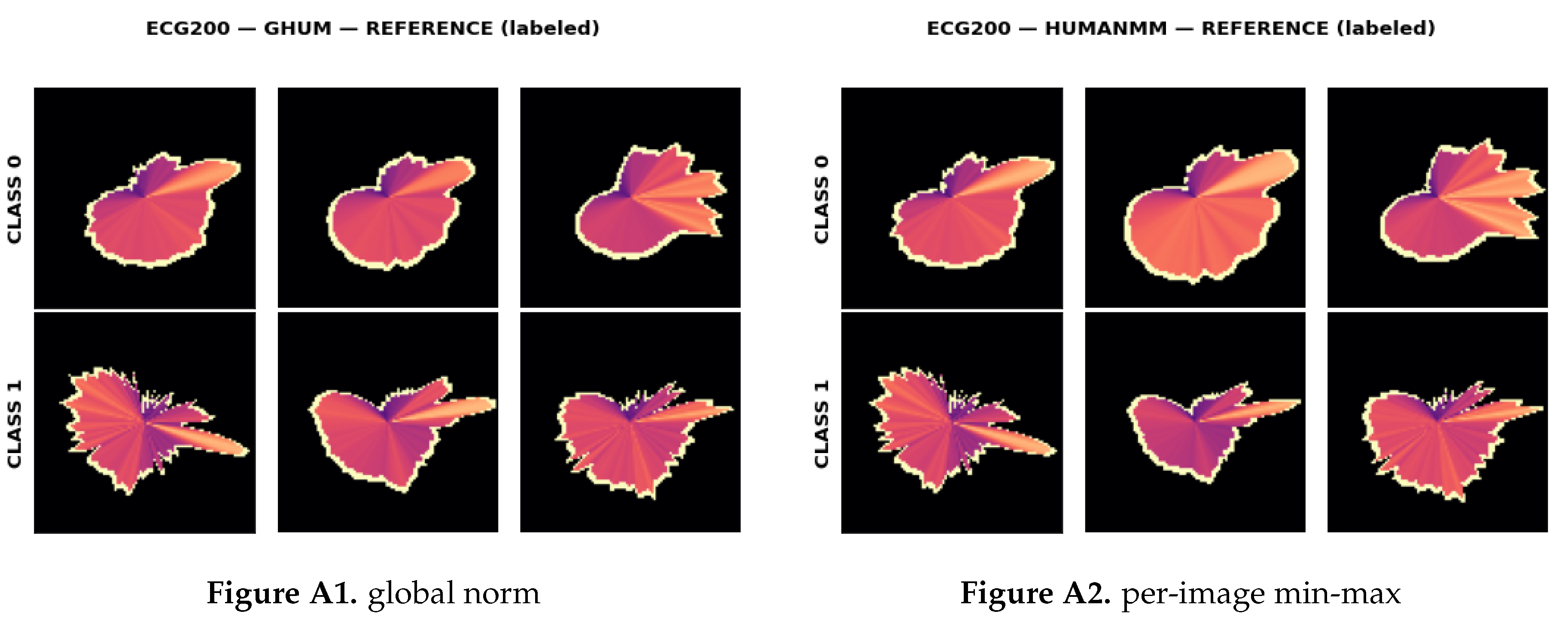
Lemma A1 has a sharper consequence for legibility. Write a sample as template plus noise, . If the template is nearly flat (range of small against the noise extremes), then : the rendered image is determined by the shape of the noise alone, stretched to full contrast, no matter how small the noise actually is. Rendered spikiness under min-max is scale-free. This is precisely the ECG200 phenomenon of Figure A1: the smooth class has small genuine ripples, min-max stretches them to the full range, and the two classes become visually indistinguishable even though their raw amplitudes differ by an order of magnitude.
Lemma A2
(Global map is uniformly Lipschitz). The global map of Equation () satisfies, for all series , , with a constant fixed once for the whole dataset.
Proof.
is -Lipschitz pointwise. □
This is principle P2 stated as mathematics: under the global map, samples close in signal space render as images close in appearance, with one dataset-wide constant. The per-image maps admit no such bound, because their gain is unbounded as the sample range shrinks; the gain diverges exactly on the smooth samples whose consistency matters most. The logistic map sits between the two: its center and scale are per-series but robust (median and MAD), so its gain varies boundedly across typical samples, which matches its intermediate legibility in Table 6 of the main paper.
Why, then, is min-max the most accurate for the network (Table A2)? The network is contrast-hungry: min-max spends the full dynamic range of every image on within-image structure, and a network trained on many samples can undo the per-image gain statistically, learning features invariant to it. The eye, shown a handful of references, cannot. The trade-off of the trade-off discussion of the main paper is thus not an accident of our encoder but a difference in what the two observers can renormalize, and it is resolved by rendering the two audiences separately.
Figure A3.
Vision reference sheets on ECG200 (rows are classes). Under global normalization (left) class 0 is a smooth rounded outline and class 1 is spiky, a stable template. Under per-image min-max (right) every sample is stretched independently, the noise becomes spikes in both classes, and the template is lost, although this is the rendering that classifies best.
Figure A3.
Vision reference sheets on ECG200 (rows are classes). Under global normalization (left) class 0 is a smooth rounded outline and class 1 is spiky, a stable template. Under per-image min-max (right) every sample is stretched independently, the noise becomes spikes in both classes, and the template is lost, although this is the rendering that classifies best.
Appendix E. Why One-Shot Nearest Neighbor Wins
The one-shot result (Table 3 of the main paper) looks surprising: a training-free rule beats a trained network by seven points on average. It follows from a metric identity.
Proposition A2
(Silhouette distance is a robust series distance). Let be unshaded filled silhouettes (Equation (A3) with constant interior) of profiles , with radius fractions and likewise. In the continuum limit the squared pixel distance is the area of the symmetric difference of the two shapes,
and since ,
with and .
Proof.
Along the spoke at angle the two indicators differ exactly for radii between and ; integrating the polar area element over that band gives , and with yields the bounds. □
Remark A2.
Interior shading () adds, over the common interior, a term per unit area; since implies , the equivalence with the profile distance survives with adjusted constants.
Proposition A2 says that Euclidean 1-NN on the encoded images is 1-NN on the normalized series under an (angle-resampled) metric. Three consequences follow.
- (a)
- The encoding embeds a good metric, it does not invent one.
This explains the close agreement between the H and raw columns of Table 2 of the main paper ( vs on average): both compute a nearest-neighbor rule on essentially the same quantity. The residual differences are attributable to the clipping of the global map, which trims outliers (a robustness gain), and to uniform angular resampling.
- (b)
- The design principles are the classical margin condition.
If P2 holds quantitatively, same-class profiles within in , and P3 holds, different-class profiles at least apart, then 1-NN classifies correctly whenever . Global normalization shrinks (Lemma A2), and the silhouette construction routes class structure into . The classical guarantee that asymptotic 1-NN risk is at most twice the Bayes risk [39] then applies to a representation engineered to have a margin, and no meta-learned embedding [41,42] is needed.
- (c)
- In the small-sample regime, zero fitting variance wins.
UCR training sets here range from tens to a few hundred series. The network fits on the order of parameters to that sample under random initialization and ordering; its seed-to-seed standard deviation reaches points (Table A2). The 1-NN rule is deterministic given the data: its variance under the training randomness is exactly zero. Once the encoder has done the invariance work, the residual statistical problem is easy, and the lowest-variance estimator wins it. This inverts the usual reading of the tables: the CNN is not the gold standard that the readable encoding approaches; on these sample sizes the CNN is the noisier instrument.
Appendix F. Cost Accounting for the Speedup
Let N be the training-set size, the test-set size, E the epoch budget, S the number of seeds, and F the multiply-accumulate cost of one forward pass. CNN training costs about (backward roughly twice forward), plus evaluation . For our network on inputs, summing the three blocks gives multiply-accumulates, so at , , the training cost is on the order of operations. The one-shot classifier costs operations total, about at : four orders of magnitude fewer arithmetic operations. The measured end-to-end wall-clock ratio of (Table 3 of the main paper) is smaller than the pure operation count because the 1-NN implementation is memory-bound while the network amortizes overhead across batches; we report the measured number. Beyond speed, the 1-NN rule needs no gradient infrastructure, no accelerator, no hyperparameters, and its prediction comes with an exhibit: the nearest training image is the explanation, in the same readable format a person can verify by eye.
Appendix G. Additional Experimental Results
This appendix collects the experiments that support the main paper but did not fit its page budget: the exploratory single-seed study that shaped GIPT, the five-seed CNN comparison on the twelve core datasets, the full component ablation, and the per-dataset tables behind the baseline and robustness summaries of the main paper.
Appendix G.1. Exploratory Study
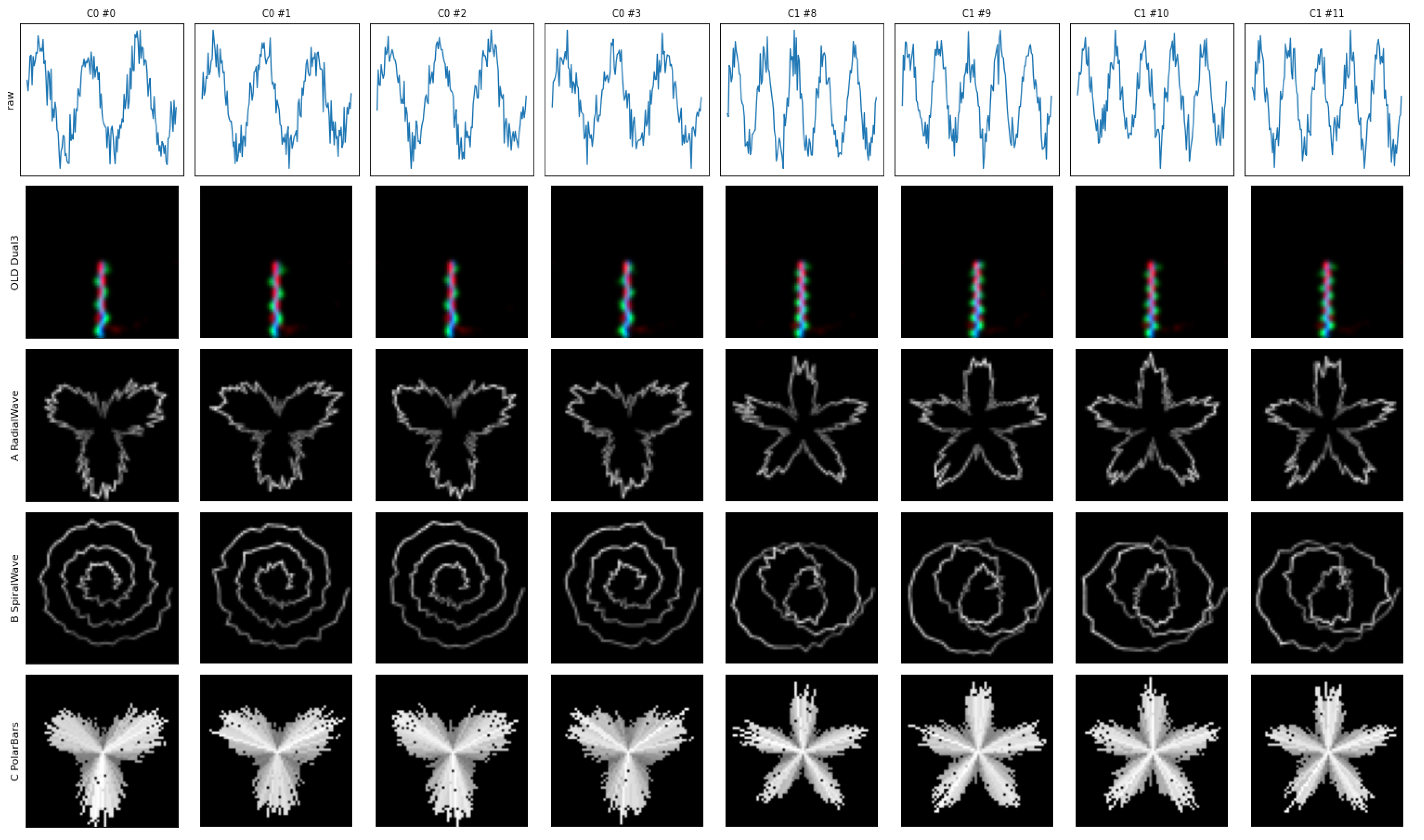
We first compared the opaque baseline against the bare axis-swapped curve and several intermediates on four datasets with a single seed (Table A1); these are the iterations that gave GIPT its name. The bare radial waveform (Curve) is very legible (Figure A2) but drops GunPoint to chance, because its thin curve and per-image normalization discard the small overshoot that defines the class. The outward spiral line (Spiral) recovers GunPoint to ; filling the silhouette (Fill) recovers Coffee and ECG; a filled spiral band with k turns (Bandk) can beat the baseline with a tuned k, but the best number of turns is dataset-dependent. These observations motivated the filled silhouette operator, the gradient channel, and the move to multi-seed evaluation.
Table A1.
Exploratory single-seed CNN accuracy (%) of the early GIPT iterations. Columns: OLD the original opaque spiral baseline; Curve a bare one-turn radial waveform (value drives the radius, thin outline only); Spiral a thin outward spiral line; Fill a filled one-turn radial silhouette; Bandk a filled spiral band with k turns. Early numbers with the original batch-normalized classifier, shown to convey the shape of the problem.
Table A1.
Exploratory single-seed CNN accuracy (%) of the early GIPT iterations. Columns: OLD the original opaque spiral baseline; Curve a bare one-turn radial waveform (value drives the radius, thin outline only); Spiral a thin outward spiral line; Fill a filled one-turn radial silhouette; Bandk a filled spiral band with k turns. Early numbers with the original batch-normalized classifier, shown to convey the shape of the problem.
| dataset | OLD | Curve | Spiral | Fill | Band4 | Band4 |
| GunPoint | 90.0 | 49.3 | 80.0 | 51.3 | 49.3 | 92.0 |
| Coffee | 53.6 | 67.9 | 57.1 | 82.1 | 100.0 | 67.9 |
| ECG200 | 85.0 | 64.0 | 64.0 | 69.0 | 64.0 | 79.0 |
| ItalyPow. | 93.7 | 81.3 | 71.3 | 61.9 | 80.0 | 50.1 |
Figure A4.
Controlled frequency experiment, 3 Hz on the left four columns and 5 Hz on the right four. Row 1 raw signal; row 2 the opaque baseline, visually identical across all eight samples; row 3 the readable radial waveform, which yields three versus five countable petals as predicted by Proposition 2; rows 4 and 5 spiral and polar-bar variants.
Figure A4.
Controlled frequency experiment, 3 Hz on the left four columns and 5 Hz on the right four. Row 1 raw signal; row 2 the opaque baseline, visually identical across all eight samples; row 3 the readable radial waveform, which yields three versus five countable petals as predicted by Proposition 2; rows 4 and 5 spiral and polar-bar variants.
Appendix G.2. Cnn Accuracy On The Twelve Core Datasets
Table A2 gives the headline comparison: the OLD baseline, GIPT-MC with min-max normalization, and its single human channel GIPT-H. GIPT-MC matches and slightly exceeds the baseline on average ( vs ) and wins on six of twelve datasets, including a perfect score on Trace. Structurally, then, a readable polar silhouette does not cost classifier accuracy.
Table A2.
CNN test accuracy on the twelve core datasets (%, mean±std over five seeds). All three columns train the same GroupNorm convolutional network for fifty epochs; only the input encoding differs. OLD: the original opaque spiral baseline. GIPT-MC: the proposed readable three-channel encoder (per-image min-max). GIPT-H: only its single human-facing channel. Bold marks the best encoder per dataset. Reading guide: GIPT-MC matching or beating OLD (six of twelve rows, and on average) is the paper’s claim that readable structure costs no accuracy.
Table A2.
CNN test accuracy on the twelve core datasets (%, mean±std over five seeds). All three columns train the same GroupNorm convolutional network for fifty epochs; only the input encoding differs. OLD: the original opaque spiral baseline. GIPT-MC: the proposed readable three-channel encoder (per-image min-max). GIPT-H: only its single human-facing channel. Bold marks the best encoder per dataset. Reading guide: GIPT-MC matching or beating OLD (six of twelve rows, and on average) is the paper’s claim that readable structure costs no accuracy.
| dataset | OLD | GIPT-MC | GIPT-H |
| GunPoint | 84.9±2.8 | 75.9±4.6 | 66.8±3.1 |
| Coffee | 74.3±17.7 | 85.0±8.9 | 60.0±9.1 |
| ECG200 | 73.4±5.4 | 75.8±0.7 | 64.0±0.6 |
| ItalyPower. | 86.2±4.0 | 64.7±4.7 | 68.2±12.1 |
| TwoLeadECG | 69.1±3.9 | 79.8±3.0 | 60.0±4.2 |
| ECGFiveDays | 72.9±2.3 | 71.6±2.7 | 64.2±0.2 |
| MoteStrain | 78.5±3.0 | 80.5±0.5 | 75.7±1.0 |
| BeetleFly | 65.0±8.4 | 55.0±6.3 | 53.0±5.1 |
| BirdChicken | 68.0±9.3 | 86.0±5.8 | 77.0±2.4 |
| Plane | 87.4±7.7 | 79.8±4.1 | 48.6±9.9 |
| Trace | 75.8±2.2 | 100.0±0.0 | 96.4±3.1 |
| Wine | 50.0±0.0 | 50.0±0.0 | 50.0±0.0 |
| average | 73.8 | 75.3 | 65.3 |
Appendix G.3. Full Component Ablation
Discussed in the ablation subsection of the main paper; all variants use the global normalization and the training-free 1-NN classifier.
Table A3.
Component ablation (% accuracy, training-free 1-NN, global normalization throughout). Outline: thin polar outline only. Fill: filled silhouette, flat interior. Shade: filled plus interior shading, which is exactly GIPT-H. MC: plus gradient and smoothed channels, which is exactly GIPT-MC.
Table A3.
Component ablation (% accuracy, training-free 1-NN, global normalization throughout). Outline: thin polar outline only. Fill: filled silhouette, flat interior. Shade: filled plus interior shading, which is exactly GIPT-H. MC: plus gradient and smoothed channels, which is exactly GIPT-MC.
| dataset | Outline | Fill | Shade | MC |
| GunPoint | 92.0 | 92.0 | 91.3 | 92.7 |
| Coffee | 96.4 | 96.4 | 96.4 | 96.4 |
| ECG200 | 89.0 | 89.0 | 90.0 | 90.0 |
| ItalyPower. | 94.2 | 95.5 | 96.2 | 95.7 |
| TwoLeadECG | 72.2 | 71.6 | 71.3 | 71.8 |
| ECGFiveDays | 76.4 | 79.1 | 80.4 | 81.1 |
| MoteStrain | 82.0 | 84.7 | 83.4 | 83.5 |
| BeetleFly | 60.0 | 65.0 | 70.0 | 65.0 |
| BirdChicken | 60.0 | 60.0 | 65.0 | 65.0 |
| Plane | 98.1 | 98.1 | 98.1 | 98.1 |
| Trace | 81.0 | 80.0 | 79.0 | 83.0 |
| Wine | 61.1 | 59.3 | 63.0 | 48.1 |
| average | 80.2 | 80.9 | 82.0 | 80.9 |
Appendix G.4. Per-Dataset Baseline and Robustness Tables
Table A4 gives the per-dataset accuracies behind the baseline comparison of the baseline-comparison subsection of the main paper, and Table A5 the per-dataset robustness curves behind Table 5 of the main paper. The DTW column uses 1-NN with a Sakoe-Chiba window of on z-normalized series [12]; the ROCKET column is the mean over three seeds of the ten-thousand-kernel classifier of [21]; the GIPT column repeats 1-NN GIPT-MC from Table 2 of the main paper for side-by-side reading.
Table A4.
Per-dataset comparison with DTW 1-NN and ROCKET (% test accuracy, identical splits). Bold marks the best of the three per row.
Table A4.
Per-dataset comparison with DTW 1-NN and ROCKET (% test accuracy, identical splits). Bold marks the best of the three per row.
| dataset | 1-NN GIPT-MC | DTW 1-NN | ROCKET |
| GunPoint | 89.3 | 94.0 | 100.0 |
| Coffee | 100.0 | 100.0 | 100.0 |
| ECG200 | 86.0 | 82.0 | 91.3 |
| ItalyPower. | 96.0 | 95.2 | 96.9 |
| TwoLeadECG | 78.2 | 89.4 | 99.9 |
| ECGFiveDays | 84.0 | 78.7 | 100.0 |
| MoteStrain | 83.0 | 86.8 | 91.6 |
| BeetleFly | 70.0 | 70.0 | 90.0 |
| BirdChicken | 65.0 | 75.0 | 90.0 |
| Plane | 99.0 | 100.0 | 100.0 |
| Trace | 100.0 | 100.0 | 100.0 |
| Wine | 61.1 | 57.4 | 82.7 |
| SonyAIBO1 | 70.7 | 73.0 | 92.4 |
| SonyAIBO2 | 84.6 | 83.3 | 92.2 |
| Chinatown | 92.1 | 95.3 | 98.2 |
| PowerCons | 91.7 | 89.4 | 94.1 |
| GunPtAgeSpan | 94.6 | 96.5 | 99.7 |
| GunPtMvF | 98.4 | 99.7 | 99.9 |
| ArrowHead | 78.3 | 72.0 | 81.3 |
| Ham | 62.9 | 49.5 | 72.1 |
| Herring | 56.2 | 53.1 | 59.9 |
| ToeSeg1 | 72.4 | 77.6 | 95.3 |
| ToeSeg2 | 76.9 | 87.7 | 92.6 |
| DistPhalanxOC | 73.9 | 71.7 | 76.7 |
| ProxPhalanxOC | 79.7 | 78.4 | 90.1 |
| Strawberry | 94.1 | 94.1 | 98.1 |
| FreezerSm | 96.3 | 75.9 | 94.9 |
| SynthControl | 93.7 | 99.3 | 100.0 |
| average | 83.1 | 83.0 | 92.1 |
Table A5.
Per-dataset noise robustness (% accuracy, training-free 1-NN, mean over three noise seeds; noise added to test series only). For each dataset the left column is 1-NN on GIPT-H global-normalized images and the right column 1-NN on the z-normalized raw series.
Table A5.
Per-dataset noise robustness (% accuracy, training-free 1-NN, mean over three noise seeds; noise added to test series only). For each dataset the left column is 1-NN on GIPT-H global-normalized images and the right column 1-NN on the z-normalized raw series.
| GunPoint | Coffee | ECG200 | ItalyPower. | |||||
| H | raw | H | raw | H | raw | H | raw | |
| 0.0 | 91.3 | 91.3 | 96.4 | 100.0 | 90.0 | 88.0 | 96.2 | 95.5 |
| 0.1 | 90.7 | 90.7 | 98.8 | 100.0 | 88.3 | 87.7 | 95.8 | 95.5 |
| 0.2 | 87.8 | 89.1 | 100.0 | 100.0 | 87.7 | 87.3 | 95.0 | 94.8 |
| 0.4 | 80.4 | 84.2 | 88.1 | 96.4 | 86.0 | 87.7 | 91.0 | 91.6 |
Appendix H. Encoder Pseudocode
| Algorithm A1 Vectorized filled silhouette |
Require: profile
, size S, radii , shade flag
|
| Algorithm A2 Aligned multi-channel encoder |
Require: series , size S, normalization mode, optional global params fit on the training pool
|
Appendix I. Hyperparameters and Reproducibility
Image size is for the readable encoders and for the baseline. Silhouette radii , . The gradient field uses a centered finite difference, the smoothed field a moving average of width . The global normalization uses the first and ninety-ninth percentiles of the pooled training values, fit once on the training split only, never on test data. The classifier uses channels, GroupNorm [46] with eight groups, Adam [47] at , batch size thirty-two, fifty epochs, no weight decay, no early stopping, no augmentation (the Experimental Setup section of the main paper explains why). All experiments use the default UCR archive train and test splits [2,28]. Accuracy is the mean over seeds (five for Table A2, three for Table 2 of the main paper); the one-shot classifier is deterministic and needs no seeds. Images are rendered once and cached, so encoder cost is shared by every classifier. All experiments run on a single consumer x86-64 CPU machine (Windows 11, no GPU) with Python 3, NumPy 2.3, PyTorch 2.12 (CPU build), aeon 1.4, and SciPy 1.17; random seeds are the integers listed with each experiment (0 to 4 for the five-seed study, 0 to 2 elsewhere), applied to network initialization, batch order, and noise draws.
Appendix J. Human Test-Set Study: Materials and Protocol
Each packet covers one dataset (Coffee, ECG200, GunPoint, ItalyPowerDemand) and contains three artifacts rendered with the most readable encoder, GIPT-H under global normalization. (1) A study sheet: several labeled training examples per class, arranged in rows by class, from which the grader learns the class templates. (2) A blind test sheet: twenty test images, numbered, shuffled, and unlabeled, drawn from the standard test split. (3) A hidden key: the true label of each test image together with the CNN prediction and the one-shot 1-NN prediction on those same twenty images, so that human, network, and nearest-neighbor accuracy are computed on an identical query set.
The protocol is deliberately committal: the grader studies the study sheet, writes a label for every numbered image on the test sheet, and only then opens the key; no revision after seeing any answer is permitted. This mirrors the vision zero-shot protocol of the Experimental Setup section of the main paper and makes the legibility claim falsifiable by any reader with the packet. For a controlled study we recommend at least ten graders per dataset, a counterbalanced order of datasets across graders, exact binomial confidence intervals on each accuracy, and McNemar tests on the paired human versus model predictions, following standard practice for paired classifier comparison [49]. The per-dataset sample of twenty queries bounds what a single grader can establish; the instrument, not any one grader’s score, is the contribution.
Appendix K. Per-Dataset Notes and Failure Cases
The expanded benchmark (Table 2 of the main paper) contains instructive extremes; we read them through the theory above.
- Trace (100% readable CNN and 1-NN).
The classes differ by a large morphological event, exactly the P3 regime; the silhouette makes it a categorical shape difference and every classifier saturates.
- Coffee (1-NN 100% on aligned, 96.4% on human).
Spectra are smooth and same-class samples nearly congruent under the global map, the small- large- margin case of Appendix E; the CNN, at to depending on encoder, is the noisier instrument at .
- GunPoint (eye-hard, machine-easy).
The class difference is a small localized overshoot. It survives in pixel space, 1-NN reaches on the human channel, but it is not a global shape difference, so vision legibility stays near chance under the global map (Table 6 of the main paper). This is the anticipated failure mode of the legibility claim: no static image makes a subtle local feature eye-separable, and the claim is conditional on morphological class structure.
- Wine (everything fails except 1-NN, modestly).
All CNN variants sit at exactly ; the one-shot rule reaches 61 to . The spectroscopic class difference is a sub-percent amplitude effect: after any rendering to a image it is at the quantization floor, and only the direct distance rule extracts a trace of it.
- FreezerSmallTrain (min-max beats global for 1-NN, 96.3 vs 72.9).
Here amplitude varies within class and shape carries the label, so the per-image map, which discards amplitude (Lemma A1), is the better metric: the invariance that destroys legibility on ECG200 is exactly the right invariance on this dataset. Normalization is a modeling choice, and the global map is the right default for legibility, not a universal optimum for accuracy.
- BirdChicken versus BeetleFly.
Both encode object outlines as series; the readable encoder helps the CNN markedly on BirdChicken ( vs baseline) but not on BeetleFly ( vs ). With twenty training series each, the seed-level noise of Appendix E(c) dominates, and the deterministic 1-NN columns ( on BirdChicken, to on BeetleFly) are the more stable comparison.
References
- Keogh, E.; Kasetty, S. On the need for time series data mining benchmarks: A survey and empirical demonstration. Data Min. Knowl. Discov. 2003, 7(4), 349–371. [Google Scholar] [CrossRef]
- Bagnall, A.; Lines, J.; Bostrom, A.; Large, J.; Keogh, E. The great time series classification bake off. Data Min. Knowl. Discov. 2017, 31(3), 606–660. [Google Scholar] [CrossRef]
- Middlehurst, M.; Schäfer, P.; Bagnall, A. Bake off redux: A review and experimental evaluation of recent time series classification algorithms. Data Min. Knowl. Discov. 2024, 38(4), 1958–2031. [Google Scholar] [CrossRef]
- LeCun, Y.; Bottou, L.; Bengio, Y.; Haffner, P. Gradient-based learning applied to document recognition. Proc. IEEE 1998, 86(11), 2278–2324. [Google Scholar] [CrossRef]
- Krizhevsky, A.; Sutskever, I.; Hinton, G. E. ImageNet classification with deep convolutional neural networks. In Advances in Neural Information Processing Systems; 2012; pp. 1097–1105. [Google Scholar]
- He, K.; Zhang, X.; Ren, S.; Sun, J. Deep residual learning for image recognition. In Proceedings of the IEEE Conference on Computer Vision and Pattern Recognition, 2016; pp. 770–778. [Google Scholar]
- Wang, Z.; Oates, T. Imaging time series to improve classification and imputation. IJCAI 2015. [Google Scholar] [CrossRef]
- Eckmann, J.-P.; Kamphorst, S. O.; Ruelle, D. Recurrence plots of dynamical systems. Europhys. Lett. 1987, 4(9), 973–977. [Google Scholar] [CrossRef]
- Marwan, N.; Romano, M. C.; Thiel, M.; Kurths, J. Recurrence plots for the analysis of complex systems. Phys. Rep. 2007, 438(5), 237–329. [Google Scholar] [CrossRef]
- Verstraete, D.; Ferrada, A.; Droguett, E. L.; Meruane, V.; Modarres, M. Deep learning enabled fault diagnosis using time-frequency image analysis of rolling element bearings. Shock and Vibration, 2017. [Google Scholar]
- Hatami, N.; Gavet, Y.; Debayle, J. Classification of time-series images using deep convolutional neural networks. In Tenth International Conference on Machine Vision (ICMV 2017); SPIE, 2018. [Google Scholar]
- Berndt, D. J.; Clifford, J. Using dynamic time warping to find patterns in time series. In KDD Workshop; AAAI Press, 1994; pp. 359–370. [Google Scholar]
- Lines, J.; Bagnall, A. Time series classification with ensembles of elastic distance measures. Data Min. Knowl. Discov. 2015, 29(3), 565–592. [Google Scholar]
- Lin, J.; Keogh, E.; Wei, L.; Lonardi, S. Experiencing SAX: A novel symbolic representation of time series. Data Min. Knowl. Discov. 2007, 15(2), 107–144. [Google Scholar] [CrossRef]
- Schäfer, P. The BOSS is concerned with time series classification in the presence of noise. Data Min. Knowl. Discov. 2015, 29(6), 1505–1530. [Google Scholar]
- Schäfer, P.; Leser, U. Fast and accurate time series classification with WEASEL. In Proceedings of the 2017 ACM Conference on Information and Knowledge Management, 2017; pp. 637–646. [Google Scholar]
- Ye, L.; Keogh, E. Time series shapelets: A new primitive for data mining. In Proceedings of the 15th ACM SIGKDD International Conference on Knowledge Discovery and Data Mining, 2009; pp. 947–956. [Google Scholar]
- Hills, J.; Lines, J.; Baranauskas, E.; Mapp, J.; Bagnall, A. Classification of time series by shapelet transformation. Data Min. Knowl. Discov. 2014, 28(4), 851–881. [Google Scholar] [CrossRef]
- Lines, J.; Taylor, S.; Bagnall, A. Time series classification with HIVE-COTE: The hierarchical vote collective of transformation-based ensembles. ACM Trans. Knowl. Discov. From Data 2018, 12(5). [Google Scholar] [CrossRef]
- Middlehurst, M.; Large, J.; Flynn, M.; Lines, J.; Bostrom, A.; Bagnall, A. HIVE-COTE 2.0: A new meta ensemble for time series classification. Mach. Learn. 2021, 110(11), 3211–3243. [Google Scholar] [CrossRef]
- Dempster, A.; Petitjean, F.; Webb, G. I. ROCKET: Exceptionally fast and accurate time series classification using random convolutional kernels. Data Min. Knowl. Discov. 2020, 34(5), 1454–1495. [Google Scholar] [CrossRef]
- Dempster, A.; Schmidt, D. F.; Webb, G. I. MiniRocket: A very fast (almost) deterministic transform for time series classification. In Proceedings of the 27th ACM SIGKDD Conference on Knowledge Discovery and Data Mining, 2021; pp. 248–257. [Google Scholar]
- Cui, Z.; Chen, W.; Chen, Y. Multi-scale convolutional neural networks for time series classification. arXiv 2016, arXiv:1603.06995. [Google Scholar]
- Wang, Z.; Yan, W.; Oates, T. Time series classification from scratch with deep neural networks: A strong baseline. International Joint Conference on Neural Networks, 2017; pp. 1578–1585. [Google Scholar]
- Karim, F.; Majumdar, S.; Darabi, H.; Chen, S. LSTM fully convolutional networks for time series classification. IEEE Access 2018, 6, 1662–1669. [Google Scholar] [CrossRef]
- Ismail Fawaz, H.; Forestier, G.; Weber, J.; Idoumghar, L.; Muller, P.-A. Deep learning for time series classification: A review. Data Min. Knowl. Discov. 2019, 33(4), 917–963. [Google Scholar] [CrossRef]
- Ismail Fawaz, H.; Lucas, B.; Forestier, G.; et al. InceptionTime: Finding AlexNet for time series classification. Data Min. Knowl. Discov. 2020, 34(6), 1936–1962. [Google Scholar] [CrossRef]
- Dau, H. A.; Bagnall, A.; Kamgar, K.; et al. The UCR time series archive. IEEE/CAA J. Autom. Sin. 2019, 6(6), 1293–1305. [Google Scholar] [CrossRef]
- Ruiz, A. P.; Flynn, M.; Large, J.; Middlehurst, M.; Bagnall, A. The great multivariate time series classification bake off: a review and experimental evaluation of recent algorithmic advances. Data Min. Knowl. Discov. 2021, 35(2), 401–449. [Google Scholar] [CrossRef] [PubMed]
- Silva, D. F.; De Souza, V. M. A.; Batista, G. E. A. P. A. Time series classification using compression distance of recurrence plots. In IEEE International Conference on Data Mining; 2013; pp. 687–696. [Google Scholar]
- Simonyan, K.; Vedaldi, A.; Zisserman, A. Deep inside convolutional networks: Visualising image classification models and saliency maps. In ICLR Workshop; 2014. [Google Scholar]
- Selvaraju, R. R.; Cogswell, M.; Das, A.; Vedantam, R.; Parikh, D.; Batra, D. Grad-CAM: Visual explanations from deep networks via gradient-based localization. In Proceedings of the IEEE International Conference on Computer Vision, 2017; pp. 618–626. [Google Scholar]
- Ribeiro, M. T.; Singh, S.; Guestrin, C. “Why should I trust you?”: Explaining the predictions of any classifier. In Proceedings of the 22nd ACM SIGKDD International Conference on Knowledge Discovery and Data Mining, 2016; pp. 1135–1144. [Google Scholar]
- Lundberg, S. M.; Lee, S.-I. A unified approach to interpreting model predictions. In Advances in Neural Information Processing Systems; 2017. [Google Scholar]
- Adebayo, J.; Gilmer, J.; Muelly, M.; Goodfellow, I.; Hardt, M.; Kim, B. Sanity checks for saliency maps. In Advances in Neural Information Processing Systems; 2018. [Google Scholar]
- Rudin, C. Stop explaining black box machine learning models for high stakes decisions and use interpretable models instead. Nat. Mach. Intell. 2019, 1(5), 206–215. [Google Scholar] [CrossRef] [PubMed]
- Doshi-Velez, F.; Kim, B. Towards a rigorous science of interpretable machine learning. arXiv 2017, arXiv:1702.08608. [Google Scholar]
- Lipton, Z. C. The mythos of model interpretability. Commun. ACM 2018, 61(10), 36–43. [Google Scholar] [CrossRef]
- Cover, T.; Hart, P. Nearest neighbor pattern classification. IEEE Trans. Inf. Theory 1967, 13(1), 21–27. [Google Scholar] [CrossRef]
- Fei-Fei, L.; Fergus, R.; Perona, P. One-shot learning of object categories. IEEE Trans. Pattern Anal. Mach. Intell. 2006, 28(4), 594–611. [Google Scholar] [CrossRef] [PubMed]
- Vinyals, O.; Blundell, C.; Lillicrap, T.; Kavukcuoglu, K.; Wierstra, D. Matching networks for one shot learning. In Advances in Neural Information Processing Systems; 2016. [Google Scholar]
- Snell, J.; Swersky, K.; Zemel, R. Prototypical networks for few-shot learning. In Advances in Neural Information Processing Systems; 2017. [Google Scholar]
- Radford, A.; Kim, J. W.; Hallacy, C.; et al. Learning transferable visual models from natural language supervision. International Conference on Machine Learning, 2021; pp. 8748–8763. [Google Scholar]
- Alayrac, J.-B.; Donahue, J.; Luc, P.; Miech, A.; et al. Flamingo: A visual language model for few-shot learning. In Advances in Neural Information Processing Systems; 2022. [Google Scholar]
- Zheng, L.; Chiang, W.-L.; Sheng, Y.; et al. Judging LLM-as-a-judge with MT-Bench and Chatbot Arena. In Advances in Neural Information Processing Systems, Datasets and Benchmarks Track; 2023. [Google Scholar]
- Wu, Y.; He, K. Group normalization. In Proceedings of the European Conference on Computer Vision., 2018. [Google Scholar]
- Kingma, D. P.; Ba, J. Adam: A method for stochastic optimization. International Conference on Learning Representations, 2015. [Google Scholar]
- Ioffe, S.; Szegedy, C. Batch normalization: Accelerating deep network training by reducing internal covariate shift. International Conference on Machine Learning, 2015; pp. 448–456. [Google Scholar]
- Demšar, J. Statistical comparisons of classifiers over multiple data sets. J. Mach. Learn. Res. 2006, 7, 1–30. [Google Scholar]
Figure 1.
The existing three-spiral encoder on GunPoint. Top row class 0, bottom row class 1, with overlaid raw signals at the left. The encoded glyph occupies a small part of the frame, and samples within one class do not resemble one another, so there is no stable per-class template for the eye to learn.
Figure 1.
The existing three-spiral encoder on GunPoint. Top row class 0, bottom row class 1, with overlaid raw signals at the left. The encoded glyph occupies a small part of the frame, and samples within one class do not resemble one another, so there is no stable per-class template for the eye to learn.
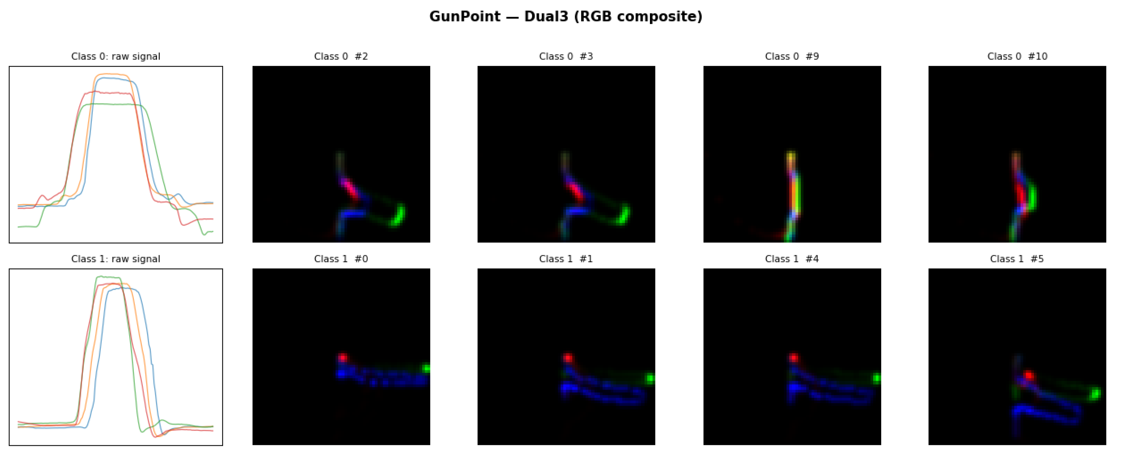
Figure 2.
GIPT-H with global normalization on two datasets, six samples per class; rows are classes. Within each row the samples are recognizably the same shape (the cross-sample consistency the OLD baseline lacked), and the difference between rows is a categorical shape feature, as required by principle P3.
Figure 2.
GIPT-H with global normalization on two datasets, six samples per class; rows are classes. Within each row the samples are recognizably the same shape (the cross-sample consistency the OLD baseline lacked), and the difference between rows is a categorical shape feature, as required by principle P3.
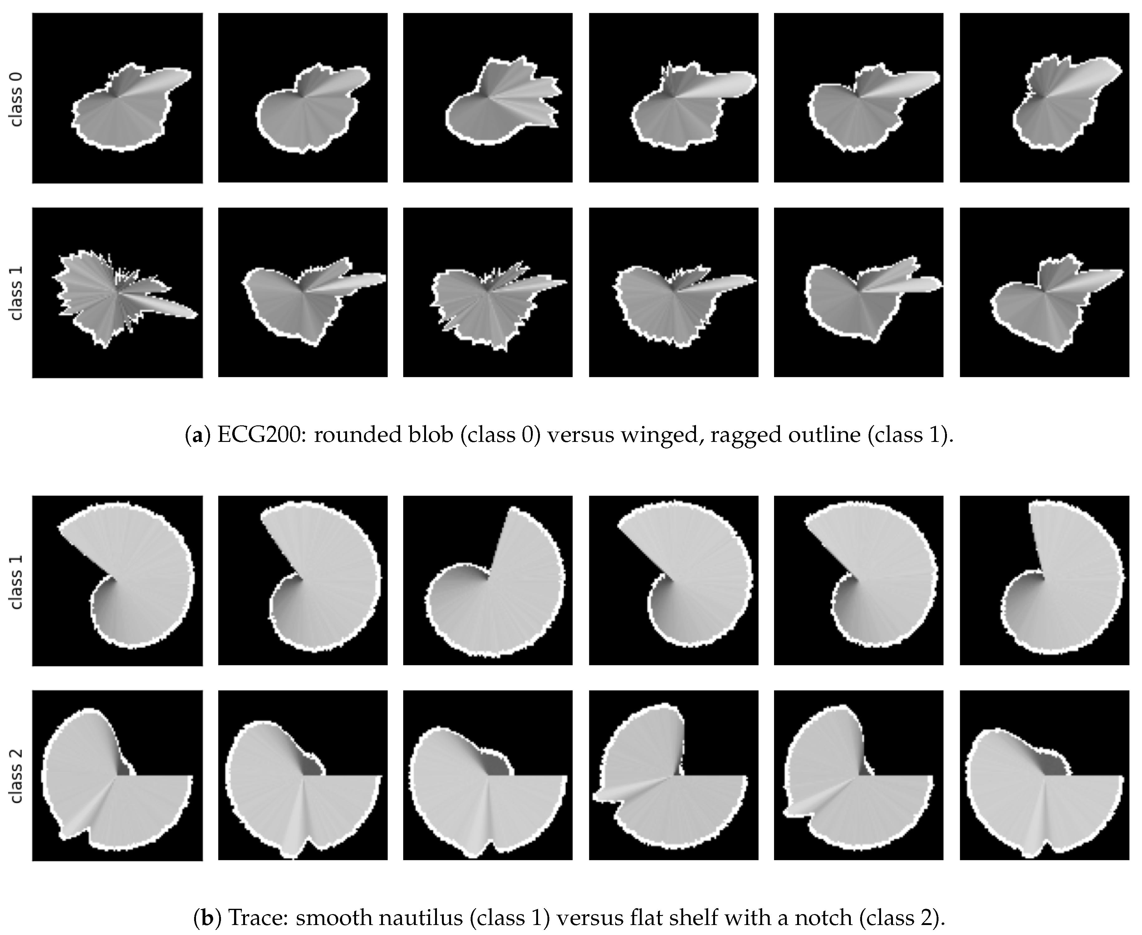
Table 1.
Notation used throughout the paper. Symbols above the first rule are shared; belong to the OLD baseline encoder only, and to the proposed GIPT encoder only.
Table 1.
Notation used throughout the paper. Symbols above the first rule are shared; belong to the OLD baseline encoder only, and to the proposed GIPT encoder only.
| symbol | meaning |
| input time series of length n | |
| time fraction of sample i, in | |
| ; | encoder; convolutional classifier |
| normalization map to (Equations 8 to 10) | |
| normalized value of sample i | |
| number of polar turns | |
| filled silhouette operator (Eq. 7) | |
| ; | OLD: robust-normalized value; time term |
| ; | OLD: plotted radius; plotted angle (Eq. 3) |
| ; | GIPT: plotted angle; plotted radius (Eq. 6) |
Table 5.
Noise robustness (% accuracy, training-free 1-NN, mean over GunPoint, Coffee, ECG200, and ItalyPowerDemand and over three noise seeds). Gaussian noise of standard deviation the per-series standard deviation is added to test series only. GIPT-H is the global-normalized silhouette; raw is the same rule on the z-normalized noisy series.
Table 5.
Noise robustness (% accuracy, training-free 1-NN, mean over GunPoint, Coffee, ECG200, and ItalyPowerDemand and over three noise seeds). Gaussian noise of standard deviation the per-series standard deviation is added to test series only. GIPT-H is the global-normalized silhouette; raw is the same rule on the z-normalized noisy series.
| 0.0 | 0.1 | 0.2 | 0.4 | |
| 1-NN GIPT-H | 93.5 | 93.4 | 92.6 | 86.4 |
| 1-NN raw | 93.7 | 93.5 | 92.8 | 90.0 |
Table 6.
Vision zero-shot legibility (% correct, sixteen queries per condition, predictions committed before scoring; higher is more legible). Columns are encoder and normalization pairs: OLD the opaque baseline, MC the GIPT-MC composite, H the GIPT-H silhouette, each rendered under the logistic, per-image min-max, or global normalization of Equations 8 to .
Table 6.
Vision zero-shot legibility (% correct, sixteen queries per condition, predictions committed before scoring; higher is more legible). Columns are encoder and normalization pairs: OLD the opaque baseline, MC the GIPT-MC composite, H the GIPT-H silhouette, each rendered under the logistic, per-image min-max, or global normalization of Equations 8 to .
| logistic / base | min-max | glob. | ||||
| dataset | OLD | MC | H | MC | H | H |
| ECG200 | 62.5 | 62.5 | 75.0 | 25.0 | 43.8 | 75.0 |
| GunPoint | 75.0 | 81.2 | 68.8 | 31.2 | 37.5 | 31.2 |
Disclaimer/Publisher’s Note: The statements, opinions and data contained in all publications are solely those of the individual author(s) and contributor(s) and not of MDPI and/or the editor(s). MDPI and/or the editor(s) disclaim responsibility for any injury to people or property resulting from any ideas, methods, instructions or products referred to in the content. |
© 2026 by the authors. Licensee MDPI, Basel, Switzerland. This article is an open access article distributed under the terms and conditions of the Creative Commons Attribution (CC BY) license (http://creativecommons.org/licenses/by/4.0/).
Copyright: This open access article is published under a Creative Commons CC BY 4.0 license, which permit the free download, distribution, and reuse, provided that the author and preprint are cited in any reuse.