

Submitted:
28 July 2026
Posted:
29 July 2026
You are already at the latest version
Abstract
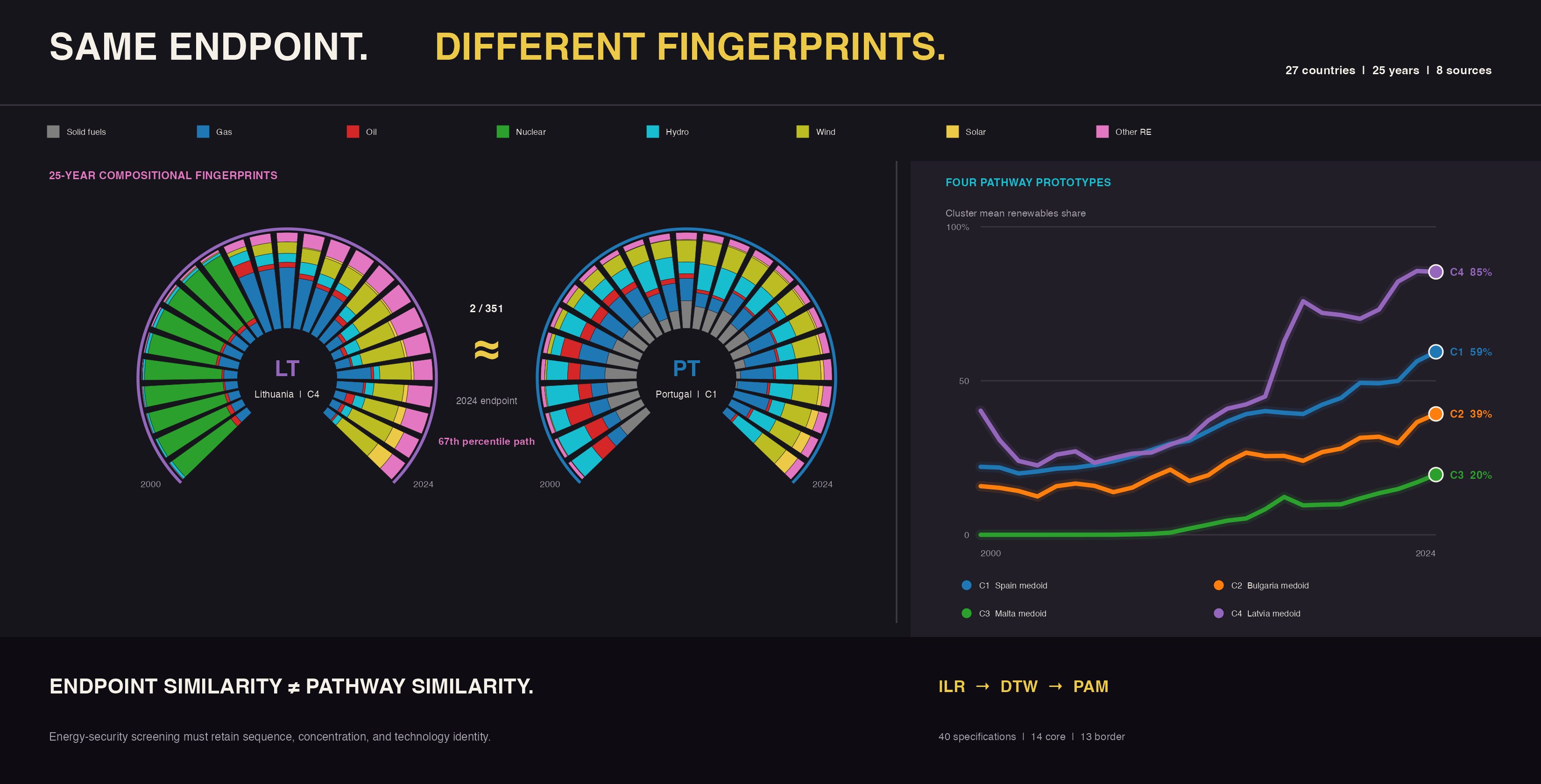
Electricity-generation mixes can converge in a final-year snapshot while following different transformation pathways, which matters for identifying energy-security exposures. This article analyzes EU-27 electricity-generation mixes for 2000–2024 (27 countries, 25 years, eight generation components) as compositional time trajectories. Shares were regularized by simple multiplicative replacement, transformed with the isometric log-ratio transformation, compared using multivariate dynamic time warping with a Sakoe–Chiba constraint, and clustered with partitioning around medoids (PAM; k-medoids). The selected four-cluster solution is represented by Spain, Bulgaria, Malta, and Latvia and describes broad renewable diversification, solid-fossil-fuel legacy transformation, high-concentration island transition, and renewable-dominant restructuring. The raw-share baseline and the compositional trajectory solution agree weakly (Adjusted Rand Index = 0.1891), while endpoint-only clustering for 2024 also diverges from full-trajectory clustering (Adjusted Rand Index = 0.1950; 10 countries change assignment after label alignment). Across 40 robustness specifications, 14 countries are core cases and 13 are border cases. This boundary sensitivity is a substantive diagnostic: stable interpretation of border countries requires information beyond generation shares. Final mix similarity is therefore not a substitute for pathway similarity, and structural energy-security exposure should be interpreted through diversification, concentration, and the sequence of fuel substitution.
Keywords:
electricity generation mix
; compositional data analysis
; dynamic time warping
; trajectory clustering
; structural energy-security exposure
; energy transition
; European Union
1. Introduction
The transformation of the electricity-generation mix is one of the most visible dimensions of the European energy transition. Over the last two decades, European Union (EU) countries have reduced the importance of some fossil-fuel components, expanded renewables, and maintained or phased out nuclear generation. These changes reflect the interaction of climate-policy objectives, technological change, energy-security conditions, fuel-price volatility, and the role of natural gas in electricity-price formation [1,2,3,4]. The energy shock that intensified in 2022 further highlighted questions about mix structure, fuel dependencies, and the geopolitical dimension of the transition [5,6].
Comparing countries by the share of a single fuel or by the level of renewables in a selected year is not sufficient to capture the logic of transformation. An electricity-generation mix is a composition: the shares of individual sources are interdependent and sum to a fixed total. It is also a trajectory, in which the starting point and endpoint matter, but so does the sequence linking them. Two countries may reach a similar renewable share in 2024 while arriving there through different fuel substitutions, rates of change, and temporary shifts in concentration.
This distinction is directly relevant to energy security. The same final renewable share may imply different exposures: a reduction in fossil-fuel dominance through broad technological diversification, the persistence of an important solid-fossil-fuel or gas component, or concentration in a narrow set of generation options. In the energy-security literature, diversification and concentration are treated as important, though not sufficient on their own, indicators of exposure [7,8,9,10]. The focus here is therefore not the general claim that diversification is inherently beneficial, but the more specific question of what kind of structural exposure remains after the electricity-generation mix has changed.
The aim of this article is to apply and evaluate an integrated framework that classifies EU-27 countries by the shape of their electricity-generation-mix transformation pathways in 2000–2024. The framework treats each country’s annual mix as a composition, transforms shares using the isometric log-ratio (ILR) transformation, and compares country trajectories as multivariate time series using dynamic time warping (DTW) distance. The final typology is obtained with partitioning around medoids (PAM)/k-medoids clustering, so each cluster has an empirical reference point in the form of an actual medoid country.
The article addresses three research questions. First, what distinct transformation pathways of the electricity-generation mix can be identified among EU countries? Second, how much do compositional geometry and temporal alignment alter the resulting typology relative to simpler representations? Third, do similar final mixes conceal different transformation pathways, and what structural energy-security exposures are indicated by these pathways?
The contribution is both methodological and empirical. Methodologically, the framework combines compositional data analysis (CoDA), multivariate DTW, and medoid clustering while separating the effects of compositional representation, temporal alignment, and endpoint-only classification. Empirically, it identifies pathway characteristics associated with distinct structural exposure profiles: high final concentration, slower phase-down of solid fossil fuels, a continuing role for gas, and rapid expansion of renewables that makes potential flexibility requirements more salient. The analysis is not a full risk model because it does not estimate event probabilities, costs, import dependence, or operational resilience; it identifies exposures visible in the structure and trajectory of electricity generation.
The remainder of the article is organized as follows. Section 2 presents the literature framework and research gap. Section 3 describes the data, fuel aggregation, and zero handling. Section 4 presents the method. Section 5 presents the typology, validation, controlled method comparison, endpoint/path diagnostic, and concentration and diversification results. Section 6 discusses the findings, and Section 7 concludes.
2. Literature Review and Research Gap
2.1. Transformation of EU Electricity-Generation Mixes
Previous research approaches the transformation of the EU electricity sector from complementary perspectives. Decomposition analyses show how changes in generation structure affect power-sector emissions [1], while system-level studies document broader shifts in the European electricity system [2]. Research on price formation and the recent energy crisis further shows that a low-carbon transition does not automatically remove exposure to fuel and price conditions, especially where natural gas remains an important fuel or price-setting mechanism [3,4,6].
Together, these studies provide the empirical background for analyzing generation-mix change, but they commonly emphasize individual indicators, policy effects, emissions, or the overall rate of renewable deployment. The question addressed here is not only whether countries reduce fossil-fuel shares, but which structural pathways they follow and whether those pathways form a stable typology.
2.2. Typologies and Clustering of Energy Pathways
Clustering is widely used in energy studies to build typologies of countries, regions, consumption profiles, and generation structures. For EU countries, previous research has examined energy pathways and transition indicators through model-based clustering [11], fuzzy-set analysis [12], similarities in renewable-energy production [13], and comparisons of conventional and renewable energy structures [14]. More recent work adds a temporal dimension through time-series analysis or dynamic time warping in assessments of sustainable energy development [15,16,17]. These studies establish the value of energy typologies, but they more often classify snapshots, summary indicators, or individual temporal profiles than complete compositional trajectories.
The study continues the author’s earlier work on empirically organizing European energy structures with clustering methods. Previous articles examined primary-energy consumption patterns in selected European countries in 1990–2021 and the structure of primary-energy production in Europe in 1990–2022 [18,19]. Those studies compared energy profiles in selected years or successive annual cross-sections rather than treating the entire course of change as one trajectory. The present analysis extends that research from primary energy to the electricity-generation mix, from cross-sectional classification to complete trajectories, and from the classical geometry of shares to log-ratio representation.
Trajectory-based typologies remain sensitive to how fuel shares are represented. Treating shares as independent Euclidean variables does not respect the fact that an increase in one part necessarily changes its relations with all others. A dynamic classification of generation mixes therefore requires both a temporal comparison and a representation appropriate for compositional data.
2.3. Compositional Data and Log-Ratio Transformations
Compositional data analysis was developed for data whose parts are interpreted relatively and sum to a fixed total. The ILR transformation maps a D-part composition isometrically into a -dimensional Euclidean coordinate space, preserving Aitchison distances [20,21,22,23]. This is directly relevant to energy mixes: the share of coal, gas, nuclear, hydro, wind, or solar has meaning in relation to the other parts rather than as an independent variable.
Compositional approaches are already used in analyses of energy structures and sustainability indicators, including the modeling of Sustainable Development Goal 7 (SDG7) indicators [24], forecasts of energy-consumption structures [25,26,27], and studies of compositional energy series [28]. The literature reviewed here, however, provides few applications that combine log-ratio representation with a dynamic comparison of complete electricity-generation-mix trajectories for EU countries.
2.4. Time-Series Clustering and Dynamic Time Warping
Dynamic time warping is an elastic measure of time-series dissimilarity that aligns sequences with similar shapes despite local shifts in timing. DTW and related measures are well established from both implementation and methodological perspectives [29,30,31]. In energy research, time-series clustering is used for dimensionality reduction in energy-system models, identification of typical system states, and comparison of temporal profiles [16,32].
In the primary specification, DTW compares the shape of multivariate ILR trajectories and therefore operates on a representation that first respects the compositional geometry of the mix. DTW on raw-share trajectories is retained only as a controlled comparator, making it possible to separate the effect of temporal alignment from the effect of compositional representation. The primary method consequently compares transformation pathways as sequences of relations among mix parts.
2.5. Diversification, Concentration, and Energy Security
The relationship between mix diversification and energy security has been present in the literature for many years. Diversification can reduce dependence on a single fuel or technology, but its interpretation depends on system context and should not be reduced to the rule that "more parts always mean less risk" [7,8,33]. Research on energy security and energy-system resilience emphasizes that mix structure is only one dimension of exposure, alongside infrastructure, imports, costs, policies, and adaptive capacity [9,10,34,35].
In this framing, Shannon diversity and the Herfindahl-Hirschman Index (HHI) describe structural characteristics relevant to energy security. A high HHI indicates that generation is concentrated in a smaller number of mix components, whereas a decline in HHI indicates a more dispersed generation structure. When declining concentration coincides with rapid renewable expansion, interpretation must also consider which technologies are added and the potential integration requirements that follow. Pathway information is therefore needed because the same final concentration level may result from different sequences of fuel substitution.
2.6. Research Gap and Positioning
The research gap lies at the intersection of four areas: EU electricity-generation mixes, energy-transition typologies, compositional data analysis, and diagnostics of structural exposure relevant to energy security. The reviewed strands separately establish the value of country typologies, DTW-based temporal comparison, and log-ratio representation. They provide fewer examples of an approach that combines these elements, evaluates them against simpler representations, and tests whether endpoint similarity is sufficient to characterize complete country pathways.
The analysis addresses this gap by combining ILR, multivariate DTW, and PAM/k-medoids in a reproducible procedure. Its purpose is not to replace existing models of energy transition, but to provide a pathway typology that respects the mathematical structure of the data and distinguishes structural exposure profiles visible in the generation mix: fossil-fuel dominance, persistence of solid fossil fuels, a continuing generation-share role for gas, rapid renewable expansion, and final concentration.
3. Data and Variable Preparation
The analysis is based on annual Eurostat data from table nrg_bal_peh, restricted to gross electricity production (GEP; nrg_bal == "GEP") and GWh (unit == "GWH") [36]. The geographic scope is defined by the current 27 European Union Member States and applied retrospectively to the entire 2000–2024 period, yielding a balanced panel of 675 country-year observations. The United Kingdom is therefore not part of the analytical sample. The EU-27 aggregate was retained as a reference series in descriptive figures and quality checks, but it was not included in clustering.
Fuel categories were constructed from a verified Standard International Energy Product Classification (SIEC) dictionary. Verification was particularly important for nuclear energy. The general code N9000 denotes a broader dictionary category of nuclear fuels and other fuels n.e.c., whereas in the analyzed nrg_bal_peh table for GEP/GWh the relevant code is N900H, or nuclear heat. The final composition has eight parts: solid fossil fuels, natural gas, oil and petroleum products, nuclear heat, hydro, wind, solar, and other renewables, biofuels and waste. Oil shale and oil sands (S2000), peat and peat products (P1000), and manufactured gases were grouped with solid fossil fuels in the analytical dictionary. As separate parts, these fuels would create highly sparse components concentrated in a small number of countries. Aggregation preserves their mass while limiting the influence of nearly empty parts on log-ratio transformations after zero replacement.
Shares were computed as the ratio of each aggregated fuel category to the sum of the eight selected categories in a given country and year. The Eurostat TOTAL row was used as an external quality-control reference, not as the denominator of the analytical composition. Across all 675 country-year observations, the median absolute relative component–TOTAL difference was 0.0071, and 96 observations exceeded the 2% diagnostic threshold. These exceedances were retained; they were not used to remove or rescale observations. The model closes exactly the eight included fuel parts, so its shares sum to 1 by construction.
Zeros were treated differently depending on analytical purpose. A reported zero can be a likely substantive, or essential, absence of a technology, but it can also reflect reporting or rounding. Nuclear heat illustrates the first case: 341 of 675 country-year values are zero, and 13 countries report zero nuclear generation throughout the full period. Isolated zeros in other components may be more ambiguous. These labels are diagnostic rather than verified Eurostat metadata classifications. Raw zeros were therefore retained in descriptive analyses and in the concentration and diversification indices.
The compositional analysis requires positive parts because log-ratio transformations compare parts through logarithms of their ratios. A zero makes these relations singular: it can produce an infinite ratio or the logarithm of zero, and one zero part prevents calculation of every log-ratio in which it participates. Replacement is consequently a numerical regularization step, not an assertion that electricity was generated from a technology reported as absent. The raw value remains zero for descriptive purposes; only the matrix entering the isometric log-ratio (ILR) transformation receives a small positive trace so that all observations can be compared in a common interior of the simplex.
The primary route used simple multiplicative replacement. It was implemented with multRepl() from zCompositions [37]. For each component, its smallest positive observed share was used as an empirical operational threshold, with frac=0.65 and z.delete=FALSE. These thresholds are not official Eurostat detection limits and do not estimate latent production. The procedure proportionally rescales positive parts and preserves their ratios while producing finite closed compositions. This common regularization was chosen to maintain one comparable compositional geometry across countries, including those with persistent substantive absences. Its influence is evaluated explicitly against alternative replacement fractions, fixed GWh pseudocounts, and a Hellinger benchmark that accommodates zeros without replacing them [38,39]. The fuel-aggregation and zero-handling decisions are presented in Table 1.
4. Methods
All data preparation, computations, diagnostics, figures, and tables were produced in R 4.5.2 [40]. The main analytical package versions were zCompositions 1.6.2, compositions 2.0.9, dtw 1.23.3, dtwclust 6.0.0, cluster 2.1.8.2, and proxy 0.4.29.
4.1. Compositional Representation
An electricity-generation mix is a composition because its parts are non-negative and sum to a fixed total. Shares therefore do not behave like independent variables, but as parts of the same closed budget. If the wind share increases by 10 percentage points, an offsetting decrease must occur in other parts of the mix, even if their physical generation does not fall by the same amount. Similarly, a fall in the gas share may mean an actual decline in gas-fired generation, faster growth of other technologies, or both processes at once. Raw shares therefore primarily contain information about relations among parts, not about independent levels of individual fuels.
For this reason, ordinary Euclidean distances computed directly on shares can mix structural change with the mechanical effect of closure to 100%. Two countries may look similar when the levels of individual mix parts are compared, yet differ substantially in their pattern of fuel substitution. The key question is whether a country moves from solid fossil fuels to wind and solar, from gas to renewables, or maintains a distinct relation between nuclear energy and the other parts of the mix. The log-ratio transformation therefore shifts the analysis from closed shares to relations among parts.
The main analysis uses the ILR transformation, which represents a composition in a Euclidean coordinate space while preserving Aitchison distances [20,21,22,23]. ILR creates a set of orthogonal coordinates that describe balances among groups of mix parts. The transformation does not add new data and does not change total production; it only changes the coordinate system to one in which distances, DTW, and clustering are computed on fuel relations rather than on shares bound by the condition that their sum equals 1.
After zero replacement in the matrix intended for ILR transformation, each country-year was described by a set of ILR coordinates. For a composition with parts, the transformation gives coordinates. The default basic ILR basis was used. The basis choice affects the meaning of individual coordinates, but it does not change distances between full compositions. ILR coordinates are not directly interpretable as individual fuels, but they support valid distance calculations between compositions.
4.2. Country Trajectories
The clustering unit is not a single year, but the full country trajectory in 2000–2024. For each country, this creates a multivariate time series with dimensions of 25 years × 7 ILR coordinates. This approach distinguishes countries that end at similar points but arrive there through different pathways from countries that have similar dynamics shifted in time. No smoothing was applied in the main analysis; a 3-year moving average appears only in selected visual layers to improve figure readability.
4.3. Distance Matrices
The main distance matrix uses multivariate DTW on full ILR trajectories and therefore compares the shape of changes in relations among mix parts. To separate the effect of representation from the effect of temporal alignment, four controlled variants were also computed. The first two variants use raw shares and compare countries either by lock-step Euclidean distance on flattened annual shares or by DTW on raw-share trajectories. The next two variants use ILR-transformed compositions and compare countries either by lock-step Euclidean distance on flattened ILR trajectories or by DTW on ILR trajectories. This 2 × 2 design makes it possible to distinguish whether changes in cluster assignment are driven primarily by compositional geometry or by elastic matching of the time dimension.
DTW compares the shape of sequences under local shifts in time and belongs to the basic class of elastic measures used in time-series clustering [29,30,31]. In the analysis of energy transition, this is particularly useful because similar changes may occur in different countries with delays of several years. The primary ILR+DTW matrix was calculated with the L2 local norm, the symmetric2 step pattern, normalized distances, sqrt.dist=TRUE, and a Sakoe–Chiba window of 4 years. In a 25-year annual series, unconstrained DTW could match structurally distant periods and treat countries as similar because they contain comparable local movements, even if those movements occur in a different historical order. The 4-year band allows for plausible delays in comparable transition episodes across countries while preventing the alignment from ignoring the chronological structure of the pathway. Path constraints, including the Sakoe–Chiba band, are a standard way to control excessive matching and the computational cost of DTW [31,41]. This configuration treats DTW as a tool for comparing trajectory shape, not as a test of causal change.
4.4. Clustering and Validation
The primary algorithm is partitioning around medoids (PAM; k-medoids). This method works directly on a distance matrix and identifies actual countries as cluster medoids, which is particularly useful with precomputed dissimilarities and non-Euclidean distances [42]. This also matters interpretively, because a medoid can be described as an empirical example of a given transformation pathway. Candidate solutions were computed for . The number of clusters was evaluated using silhouette, the Dunn index, an auxiliary gap statistic, the presence of singletons, and resampling stability measured by Jaccard coefficients [43,44,45,46].
The selection rule first retained solutions without singleton clusters and without cluster-level Jaccard coefficients below 0.6, and then selected the eligible solution with the highest mean silhouette. Dunn was used as supporting evidence. The gap statistic was treated as auxiliary because it was computed after principal coordinates analysis (PCoA) of the DTW matrix with an additive correction and retention of positive axes, rather than directly on the non-Euclidean matrix. It used 100 Monte Carlo replications, and both the one-standard-error and global-maximum recommendations were recorded. Stability was evaluated with 100 bootstrap-induced unique-subset replications: countries were sampled with replacement, duplicate draws were removed before PAM clustering, and recovered clusters were matched to the full solution by their maximum Jaccard overlap, following the logic of cluster-stability assessment by resampling [46]. Deterministic seeds were derived from the central seed 20240101.
4.5. Method Comparison and Endpoint Diagnostic
To test whether the compositional-dynamic representation changes the typology, cluster solutions were compared with the Adjusted Rand Index (ARI). ARI measures partition agreement corrected for chance and remains a standard tool for comparing clustering solutions [47,48]. ARI was computed for the four controlled variants: raw shares with lock-step Euclidean distance, raw shares with DTW, ILR with lock-step Euclidean distance, and ILR with DTW. To identify the specific countries that change assignment, cluster labels in the comparison methods were aligned with the labels in the primary ILR+DTW solution so as to maximize the number of matching countries.
A separate endpoint diagnostic was used to test whether similarity in the final 2024 mix is sufficient to reproduce similarity in the full transformation pathway. For this purpose, country compositions in 2024 were transformed with ILR and clustered with PAM using Euclidean distances between endpoint compositions and the same number of clusters as in the primary trajectory solution. The endpoint-only partition was then compared with the primary full-trajectory partition by ARI and by a cluster crosswalk. Pairwise endpoint distances were also compared with full-path distances, both expressed as percentiles, to identify pairs of countries that are relatively close in 2024 but relatively distant over the entire 2000–2024 pathway.
4.6. Robustness and Sensitivity Analysis
Zero sensitivity was evaluated before the broader robustness analysis. The primary simple multiplicative replacement with frac=0.65 was compared with alternatives using frac values of 0.25 and 0.50; fixed pseudocounts of 0.01, 0.1, and 1 GWh followed by closure and ILR transformation; and a zero-tolerant Hellinger representation of raw shares. Hellinger leaves reported zeros unchanged but changes the representation, so it was treated as a benchmark for persistent substantive absences rather than as a pure replacement alternative. For each route, PAM was applied at the selected primary value of k, and partitions, medoids, internal validation metrics, and ARI relative to the primary partition were recorded.
The broader grid contained 40 specifications. It combined three aggregation dictionaries, three common zero-handling routes, and Sakoe–Chiba windows of 0, 2, 4, and 6 years; the primary eight-part simple multiplicative route was additionally evaluated at all four window widths. The six-part dictionary combined wind, solar, and other renewables, biofuels and waste into one non-hydro renewable component; the ten-part dictionary separated oil shale and oil sands and peat from the broader solid-fossil-fuel component; and the eight-part dictionary retained the primary aggregation. The three common routes were multiplicative replacement with frac=0.50, a 0.1 GWh pseudocount, and Hellinger-transformed raw shares. Window 0 enforced lock-step alignment. All solutions used the selected primary value of k, and labels were aligned to the primary partition by maximum overlap before ARI and assignment frequencies were calculated. A country was classified as a core case when its modal aligned assignment occurred in at least 80% of specifications; otherwise, it was classified as a border case. These labels summarize specification sensitivity rather than membership probabilities or ground truth.
4.7. Concentration, Diversification, and Energy-Security Exposure
The concentration and diversification layer uses Shannon diversity, normalized Shannon diversity, HHI, and the effective number of parts. For country and year, denotes the share of the i-th mix part, where and D is the number of fuel categories. Shannon diversity was computed as follows:
This measure increases when the mix is more evenly distributed among several parts; it reaches 0 when all production is assigned to one category. To facilitate comparison, normalized Shannon diversity was also used:
Its values range from 0 to 1. On this scale, 0 denotes complete dominance of one category, while 1 denotes a perfectly even split among all D parts. HHI was computed as follows:
Unlike Shannon diversity, HHI increases with mix concentration: a value close to 1 means dominance of one part, whereas lower values mean production is distributed among a larger number of categories. The effective number of parts was defined as the inverse of HHI:
With eight equal parts, the minimum HHI equals 0.125, whereas complete dominance by one part gives an HHI equal to 1. These measures were computed on reported raw shares rather than on zero-replaced data, because a reported zero remains empirically meaningful for descriptive indices whether it reflects a likely substantive absence or possible reporting or rounding. Cluster means were computed as unweighted averages across countries, so that they describe the typical country pathway within a cluster rather than the cluster’s share in total EU electricity production. Such indicators are often used as synthetic measures of diversity and concentration in energy-security analyses [7,8,33].
In the energy-security interpretation, these measures are not treated as a standalone risk assessment, but as information about the structure of exposure. A high HHI indicates that the mix depends on a small number of parts. A low HHI and high Shannon indicate more dispersed generation, but they do not automatically imply lower risk because the nature of the dominant technologies also matters. In the results below, concentration outcomes are therefore linked to the type of cluster pathway: diversification based on reductions in oil and solid fossil fuels is interpreted differently from the persistence of a substantial gas share or a rapid rise in wind and solar that may make balancing and flexibility requirements more salient [9,10,34,35].
5. Results
5.1. Descriptive Evolution of Electricity-Generation Mixes
The first layer of results shows that the European transformation has a common direction but a heterogeneous course. Figure 1 compares the EU-27 aggregate with four large electricity systems selected to provide descriptive context before the clustering results are introduced: Germany, France, Italy, and Poland. These countries are not treated as cluster representatives in this figure. Rather, they illustrate major structural contrasts in the European generation landscape: a large fossil-to-renewables transition, a nuclear-dominant system, a gas-and-renewables system, and a solid-fossil-fuel legacy system. In the EU-27 aggregate, the share of solid fossil fuels fell by 21.23 percentage points between 2000 and 2024, while the wind share increased by 17.78 percentage points and the solar share by 11.70 percentage points. Country trajectories show, however, that different sequences of fuel substitution and different rates of diversification lie beneath this common direction.
5.2. Main Typology of Transformation Pathways
Applying the selection rule yields a primary ILR+DTW trajectory solution with four clusters and Spain, Bulgaria, Malta, and Latvia as medoids. The answer to the first research question is therefore not a single axis of transformation, but four distinct empirical pathways. They differ in starting point, pace of fuel substitution, and final mix structure. The clusters should consequently be interpreted not as a ranking of transition advancement, but as four different patterns of electricity-generation-mix restructuring.
Cluster 1, represented by Spain, is a broad pattern of renewable diversification. It includes 13 countries from Western, Northern, and Southern Europe, ranging from systems with important hydro or nuclear components to those expanding wind and solar more rapidly. The average profile shifts from a mix in which fossil fuels accounted for 57.2% in 2000 to one in which renewables account for 59.4% in 2024. This is not a one-for-one replacement by a single technology: wind is the largest average component in 2024 (24.5%), but gas (19.1%), hydro (15.6%), and nuclear (15.3%) remain important. C1 therefore captures a broad substitution pathway in which the decline of solid fossil fuels and oil is distributed across several technologies.
Cluster 2, represented by Bulgaria, includes nine countries mainly from Central and Eastern Europe: Bulgaria, Croatia, Czechia, Estonia, Hungary, Poland, Romania, Slovakia, and Slovenia. Its pathway combines a solid-fossil-fuel legacy with partial diversification. In 2000, the average fossil-fuel share was 61.7%, with solid fossil fuels accounting for 48.7%. By 2024, the fossil-fuel share falls to 34.0%, but solid fossil fuels remain important (22.9%), and nuclear is the largest single component of the average profile (26.8%). Renewables rise from 15.8% to 39.3%, a smaller increase than in C1 and C4. C2 is therefore not merely a delayed version of C1: it retains a larger solid-fossil-fuel component and stronger nuclear and hydro roles throughout the transformation.
Cluster 3, represented by Malta, includes Cyprus and Malta. It is small but distinctive and stable: its bootstrap Jaccard is 0.8833, and its mean silhouette is the highest among the four clusters. This island pathway starts from a near-single-fuel mix. In 2000, the average fossil-fuel share was 100%, effectively oil, and normalized Shannon diversity was 0. By 2024, diversification occurs especially through gas (42.1%) and solar (17.1%), but fossil fuels still account for 80.5% of the average mix and HHI remains the highest in the typology (0.6764). C3 therefore separates improvement relative to the starting point from the level of concentration that remains at the endpoint.
Cluster 4, represented by Latvia, includes Latvia, Lithuania, and Luxembourg and forms a small pathway of strong renewable expansion. Its bootstrap Jaccard of 0.8400 indicates stability under resampling within the primary specification, although all three members are border cases in the broader specification grid. In 2000, renewables accounted for 40.3% of the average profile, fossil fuels for 34.5%, and nuclear for 25.2%. By 2024, renewables rise to 85.4%, fossil fuels fall to 14.6%, and nuclear disappears from the cluster average. The renewable structure remains multi-technology: wind accounts for 27.1%, hydro for 21.1%, other renewables, biofuels and waste for 20.2%, and solar for 17.0%. C4 thus represents deep restructuring without replacing the earlier mix by one dominant renewable component, but its exact membership is specification-sensitive.
The four clusters therefore distinguish broad multi-technology diversification, persistence of a solid-fossil-fuel legacy, concentrated island transformation, and renewable-dominant restructuring. Their implications for structural energy-security exposure are compared after the validation and concentration results are presented.
Figure 2 condenses the eight-part mixes into three technology groups: fossil fuels, nuclear, and renewables. Grey vectors connect each country’s 2000 and 2024 positions, while thick colored lines retain the annual ordering through 3-year moving averages of cluster means. The figure therefore adds direction and intermediate movement to the endpoint comparison: C1 and C2 both move toward renewables but remain separated by the persistence of fossil and nuclear components, C3 moves away from the fossil vertex without approaching the diversification of the other clusters, and C4 shows the strongest movement toward the renewable vertex. Smoothing is used only in this visual layer and does not affect clustering or reported metrics.
Average cluster mix profiles are shown in Figure 3, and their geographic distribution in Figure 4. Cluster composition, medoids, and basic validation metrics are reported in Table 2.
Within-cluster heterogeneity is shown in Figure 5. Thin lines correspond to individual countries, dashed lines to medoids, and thick lines to cluster means. C1 and C2 contain visibly dispersed country trajectories, whereas C3 is compact and C4 combines a common renewable direction with differences in concentration. The figure thus provides a visual counterpart to the low cluster-level silhouettes reported below: the groups summarize recurring pathway shapes without implying that all members follow a single smooth average.
5.3. Validation of the Four-Cluster Solution
Applying the stated eligibility and selection rule identifies . The selected solution has a mean silhouette of 0.1828, a Dunn index of 0.1973, an auxiliary gap statistic of 0.1845, and a minimum cluster-level Jaccard of 0.6329. Across , it is the only solution without singletons and without a Jaccard coefficient below 0.6, and it also has the highest mean silhouette. Some larger values of k yield higher Dunn or gap values, but they introduce singleton or weakly stable clusters. The gap diagnostic does not independently select four clusters: the one-standard-error rule recommends , whereas the global maximum occurs at . It is therefore reported as an auxiliary diagnostic rather than as confirmation of the selected solution. Cluster-specific stability is summarized in Table 2, with the lowest Jaccard in C2 (0.6329) and the highest in C3 (0.8833). Figure 6 presents the metrics across all candidate values of k.
The mean silhouette of 0.1828 indicates weak separation between pathways. Although fixed thresholds should not be transferred mechanically across dissimilarity measures, the low value remains evidence that several countries are nearly as close to another cluster as to their assigned cluster. This is most visible in C1 and C2, whose mean silhouettes are 0.1821 and 0.1321 and whose minima are 0.0314 and 0.0187, respectively. The result is consistent with the dispersed trajectories in Figure 5 and with the border-country analysis below. The four-cluster solution should therefore be read as a stability-constrained descriptive typology with overlapping boundaries, not as evidence for four sharply separated country populations.
Figure 7 shows country-level silhouette widths for the primary compositional trajectory solution. The dashed line marks the overall mean of 0.1828. Low positive values indicate that many countries lie close to a neighboring pathway, while the absence of negative values means that no country is, on this diagnostic, closer on average to another cluster than to its assigned cluster.
5.4. Method Comparison
The controlled method comparison shows that representation of the mix is more consequential than DTW by itself. The two raw-share variants, lock-step Euclidean and DTW, produce identical partitions (ARI = 1.0000). Thus, within raw-share geometry, elastic temporal alignment does not alter the classification. Agreement between raw-share and ILR partitions is low under both lock-step comparison (ARI = 0.1477) and DTW (ARI = 0.1891). Within the ILR representation, DTW still changes some assignments, but the agreement is substantially higher (ARI = 0.7745).
The comparison between the raw-share lock-step baseline and the primary ILR+DTW solution gives ARI = 0.1891. After optimal label alignment, 10 of 27 countries change assignment: Austria, Sweden, Bulgaria, Croatia, Hungary, Romania, Slovakia, Slovenia, Lithuania, and Luxembourg. Six of these countries – Bulgaria, Croatia, Hungary, Romania, Slovakia, and Slovenia – are assigned in the primary solution to C2, the solid-fossil-fuel legacy pathway. The difference is therefore substantive rather than a relabeling effect: raw-share geometry and compositional trajectory geometry do not isolate the same pathway groups.
Agreement among the controlled variants is shown in Figure 8. The figure answers the second research question directly: the typology changes mainly because the mix is treated as a composition, not merely because trajectories are compared with an elastic time-series distance.
Zero sensitivity is low within the multiplicative replacement family but high across conceptually different routes. Alternative multRepl fractions reproduce the primary partition exactly (minimum ARI = 1.0000), although the 0.50 variant selects Cyprus rather than Malta as the C3 medoid. In contrast, the three GWh pseudocount routes give ARI = 0.2340, and the Hellinger benchmark, which retains zeros, gives ARI = 0.1971. The pseudocount partitions also have substantially higher internal silhouette (0.4301–0.5164) and Dunn values (0.6969–0.7668) than the primary specification. A fixed addition measured in GWh is not scale-invariant after closure: it leaves a larger relative trace in a small electricity system than in a large one. Its higher apparent separation can therefore partly reflect size-dependent regularization rather than a better pathway typology. The evidence supports stability within the intended multiplicative replacement family, but the different Hellinger partition shows that the treatment of persistent substantive absences remains consequential.
The broader robustness grid confirms that the complete partition is specification-sensitive. Across 40 combinations of aggregation, zero handling, and DTW window width, the median ARI relative to the primary partition is 0.2340 and the minimum is 0.1310. Stability is concentrated in 14 core countries, whereas 13 countries do not reach the 80% modal-assignment threshold. The border cases are Estonia, Spain, Poland, Germany, Luxembourg, Lithuania, Finland, Sweden, Netherlands, Latvia, Croatia, Belgium, and France. This near-even division is a substantive result rather than a failed replication of the typology. Core cases provide its most consistent pathway prototypes; stable interpretation of border cases requires country-specific evidence beyond annual generation shares, such as capacity, interconnection, imports, flexibility, and policy commitments.
5.5. Endpoint Similarity and Full-Path Difference
The endpoint-only diagnostic confirms that the final mix is not enough to reproduce the full pathway typology. Clustering countries only by their 2024 ILR composition gives low agreement with the primary trajectory solution (ARI = 0.1950), and 10 countries change assignment after label alignment. This result answers the pathway component of the third research question: similar destinations may conceal different transformation paths. The corresponding structural exposure profiles are evaluated in the concentration results below.
Figure 9 shows this result in two ways. Panel A compares pairwise distances between 2024 endpoint compositions with pairwise distances between complete 2000–2024 trajectories. Points above the diagonal identify country pairs that are relatively close in 2024 but relatively distant over the full pathway. The strongest examples include Lithuania–Portugal, Germany–Estonia, Germany–Croatia, Latvia–Portugal, and Germany–Ireland. Panel B shows the crosswalk between endpoint-only clusters and full-trajectory clusters. The endpoint solution splits the trajectory clusters differently, especially for the broad C1 and solid-fossil-fuel legacy C2 pathways. The substantive implication is that a 2024 snapshot can obscure whether similar final shares were reached through gradual diversification, persistence of solid fossil fuels, a stronger gas role, or rapid renewable restructuring.
5.6. Diversification, Concentration, and Energy-Security Exposure
All four clusters diversify between 2000 and 2024. The scale and meaning of diversification, however, differ markedly. C3, represented by Malta, records the largest increase in normalized Shannon diversity () and the largest decline in HHI (), but remains the most concentrated cluster in 2024 (HHI = 0.6764). C4, represented by Latvia, has the largest increase in the effective number of parts () and the largest increase in the renewable share (). C2 diversifies strongly from a high level of solid-fossil-fuel concentration: normalized Shannon increases by 0.2379 and HHI falls by 0.1944. C1, the largest group of countries, diversifies more moderately: normalized Shannon increases by 0.1232, HHI falls by 0.0840, and the renewable share increases by 0.3734. A common direction of diversification therefore does not imply a similar final level of concentration or a similar rate of change.
The most important energy-security implication does not follow from diversification itself, but from the positions in which clusters end after that change. C3 reduces HHI the most, but still has HHI = 0.6764 and a fossil-fuel share of 80.5%, so it remains a high fuel-concentration profile. C2 reduces concentration strongly, but retains an important solid-fossil-fuel component, indicating continuing regulatory-emissions and investment exposure associated with its replacement. C1 reaches a lower level of concentration, but gas still accounts for 19.1% of its final profile and wind is the largest part of the mix, shifting attention from solid-fossil-fuel exposure to gas exposure and potential integration requirements for variable sources. C4 has the lowest generation-share exposure to fossil fuels, but interpretation of this pathway depends more strongly on unobserved flexibility and balancing conditions.
Figure 10 contrasts the starting and ending positions of the four clusters in normalized Shannon diversity and HHI. This compact view separates the magnitude of change from the final concentration level, while the complete within-cluster time trajectories are shown in Figure 5. Exact index changes are summarized in Table 3.
Figure 11 maps country-level structural concentration exposure rather than general energy-security risk. The horizontal axis shows HHI in 2024, and the vertical axis shows its change between 2000 and 2024. HHI falls in 23 of 27 countries. Among the other four countries, Denmark, Finland, and Ireland are classified as concentrating. Slovakia is classified as mixed or stable because its Shannon and HHI signals diverge. Cyprus and Malta remain on the right side of the figure as cases of high final concentration despite improvement from their starting point. Poland and Estonia show strong HHI declines but remain in the primary C2 pathway, where the identity of the components being replaced matters alongside concentration itself. Estonia requires particular caution: its modal aligned cluster appears in only 37.5% of robustness specifications, making its primary C2 membership especially sensitive to the aggregation of oil shale and peat and to other analytical choices.
6. Discussion
The European electricity transition does not follow a single progression from fossil fuels to renewables. Earlier typologies established that countries can be grouped by energy indicators, technology shares, or transition dynamics [11,12,16]; the present analysis adds a distinction between similarity of destinations and similarity of paths. Lithuania and Portugal, for example, are relatively close in the 2024 endpoint comparison but substantially farther apart when their complete trajectories are considered. Their contrast shows how a final-year snapshot can conceal differences in the sequence and timing of substitution. The object being classified is therefore not merely the final mix, but the transformation process that produced it.
The controlled comparison clarifies why this typology differs from simpler classifications. DTW does not alter the partition within raw-share geometry, whereas agreement between the raw-share baseline and the primary ILR+DTW solution is low (ARI = 0.1891). This does not make raw shares intrinsically unsuitable. Euclidean raw-share geometry emphasizes absolute percentage-point differences under the closure constraint, while ILR geometry emphasizes proportional relations among components and makes substitution patterns part of the comparison. DTW then evaluates how the chosen representation evolves while allowing bounded differences in timing. In the controlled design used here, representation changes the typology more than temporal alignment; elastic matching cannot recover relative information that the representation itself does not encode.
The sensitivity analysis distinguishes stability within a method family from robustness to a change in representation. Alternative multiplicative-replacement fractions reproduce the primary partition, indicating that the intensity of the positive trace is not decisive within this family. The different Hellinger partition shows, however, that the typology is not invariant to the more fundamental choice between regularizing likely substantive absences and retaining them as zeros. Across the broader grid, stability is concentrated in 14 core countries, while 13 border countries move between pathways under reasonable changes in aggregation, zero handling, or the DTW window. Border status does not imply an unknown true cluster; it indicates that the mix-only typology does not support a specification-invariant assignment. External evidence is therefore needed to interpret these countries’ energy-security exposures, not merely to validate cluster membership. This distinction also clarifies the two small clusters: C3 remains a comparatively consistent island pattern, whereas all C4 countries are border cases despite passing the cluster-level bootstrap threshold in the primary specification. The four groups are best interpreted as pathway prototypes with unequal certainty at their boundaries.
The energy-security meaning of the typology emerges only when three dimensions are read together: the direction of diversification, final concentration, and the identity of the remaining components. This interpretation is consistent with research treating diversity as an important but context-dependent dimension of energy security [7,8,33]. C3 illustrates that the largest decline in HHI can coexist with the highest final concentration and continued fossil-fuel dominance. C2 shows that greater diversity may still leave a substantial solid-fossil-fuel component. In C1 and the renewable-dominant C4 prototype, lower fossil-fuel dominance shifts the screening question toward the remaining role of gas, where present, and toward potential flexibility needs, although annual generation shares cannot determine whether those needs are adequately met. These contrasts represent different structural exposures rather than a ranking of transition performance. The typology can therefore support their identification and comparative assessment, but it does not estimate failure probabilities or prescribe risk treatment. Infrastructure, import dependence, prices, policy capacity, and system adaptability remain outside the data [9,10,34,35].
These interpretations are bounded by both the data and the analytical design. Gross electricity production is not equivalent to installed capacity, consumption, cross-border exchange, or operational adequacy, and annual observations suppress seasonal and short-run stresses. The 2022 crisis remains relevant context, particularly for gas exposure, but annual generation shares cannot support a causal or probabilistic assessment of resilience to that shock. Positive traces inserted for likely substantive zeros are an analytical regularization, not evidence of latent generation, and the Hellinger comparison shows that this choice affects the resulting typology. Aggregation and DTW constraints likewise shape the geometry of comparison without eliminating specification sensitivity. The framework should therefore be used to screen and compare pathways and to identify cases requiring deeper investigation, not as a complete model of transition causes or operational energy security.
7. Conclusions
This article develops a framework for clustering compositional trajectories of EU electricity-generation mixes in 2000–2024. The selected solution distinguishes four pathways represented by Spain, Bulgaria, Malta, and Latvia: broad multi-technology diversification, transformation with a solid-fossil-fuel legacy, a high-concentration island pathway, and renewable-dominant restructuring. These groups are recurring pathway prototypes rather than discrete country populations, as indicated by their weak separation and unequal membership stability.
The controlled comparisons answer the central methodological questions. The raw-share baseline and the ILR+DTW solution have low agreement (ARI = 0.1891), with 10 countries changing assignment, while the two raw-share variants produce identical partitions. In the controlled design used here, compositional geometry is therefore the principal source of typological change, although temporal alignment also matters within the ILR representation. Endpoint-only clustering likewise has low agreement with the full-trajectory solution (ARI = 0.1950) and changes 10 assignments. A similar destination is consequently not sufficient evidence of a similar transition: the sequence, timing, and relational pattern of fuel substitution carry information that a final-year mix omits.
Diversification must be interpreted jointly with final concentration and the identity of the remaining mix components. A pathway may diversify while remaining highly concentrated and fossil-fuel dominant, as in C3, or while retaining a solid-fossil-fuel legacy, as in C2. Lower fossil-fuel dominance in C1 and the C4 prototype instead shifts attention toward any remaining gas exposure and toward flexibility questions that cannot be resolved from annual generation shares alone. These are different structural exposures, not a single ranking of transition performance. The robustness grid further identifies 14 core and 13 border countries. Border status marks where the mix-only typology is conditional on specification; it does not imply that a single true membership can be recovered from additional data. The typology should therefore support comparative screening and risk identification, not be interpreted as a probability model or a complete assessment of energy security.
Future research should connect these pathways to fuel imports, interconnection, installed capacity, prices, flexibility resources, and reliability indicators, and should test them at frequencies capable of representing seasonal operation and short-run shocks. Combining those data with the present structural typology would permit a fuller assessment of exposure, adaptive capacity, and possible risk treatment while preserving the distinction between evidence derived from the generation mix and conclusions requiring broader system information. For comparative energy-security screening, the path to an electricity mix is therefore analytically distinct from the destination itself.
Funding
This research received no external funding.
Data Availability Statement
The study uses publicly available Eurostat data. The reproducible analysis pipeline and derived artefacts are maintained in the project repository.
Acknowledgments
AI tools were used to support coding workflow (Codex 5.5), and language editing (ChatGPT 5.5). The author remains responsible for all analytical decisions, interpretations, and final text.
Conflicts of Interest
The author declares no conflict of interest.
Abbreviations
The following abbreviations are used in this manuscript:
| ARI | Adjusted Rand Index |
| CoDA | Compositional Data Analysis |
| DTW | Dynamic Time Warping |
| EU | European Union |
| GEP | Gross Electricity Production |
| HHI | Herfindahl-Hirschman Index |
| ILR | Isometric Log-Ratio |
| PAM | Partitioning Around Medoids |
| PCoA | Principal Coordinates Analysis |
| SDG7 | Sustainable Development Goal 7 |
| SIEC | Standard International Energy Product Classification |
References
- Rodrigues, J.F.D.; Wang, J.; Behrens, P.; de Boer, P. Drivers of CO2 Emissions from Electricity Generation in the European Union 2000–2015. Renew. Sustain. Energy Rev. 2020, 133, 110104. [Google Scholar] [CrossRef]
- Koval, V.; Khaustova, V.; Lippolis, S.; Ilyash, O.; Salashenko, T.; Olczak, P. Fundamental Shifts in the Eu’s Electric Power Sector Development: LMDI Decomposition Analysis. Energies 2023, 16, 5478. [Google Scholar] [CrossRef]
- Zakeri, B.; Staffell, I.; Dodds, P.; Grubb, M.; Ekins, P.; Jääskeläinen, J.; Cross, S.; Helin, K.; Gissey, G.C. The Role of Natural Gas in Setting Electricity Prices in Europe. Energy Rep. 2023, 10, 2778–2792. [Google Scholar] [CrossRef]
- Urbano, E.; Kampouropoulos, K.; Romeral, L. Energy Crisis in Europe: The European Union’s Objectives and Countries’ Policy Trends—New Transition Paths? Energies 2023, 16, 5957. [Google Scholar] [CrossRef]
- Borowski, P. Mitigating Climate Change and the Development of Green Energy versus a Return to Fossil Fuels Due to the Energy Crisis in 2022. Energies 2022, 15, 9289. [Google Scholar] [CrossRef]
- Goldthau, A.C.; Youngs, R. The EU Energy Crisis and a New Geopolitics of Climate Transition. JCMS J. Common Mark. Stud. 2023, 61, 115–124. [Google Scholar] [CrossRef]
- Grubb, M.; Butler, L.; Twomey, P. Diversity and Security in UK Electricity Generation: The Influence of Low Carbon Objectives. Energy Policy 2006, 34, 4050–4062. [Google Scholar] [CrossRef]
- Chalvatzis, K.; Ioannidis, A. Energy Supply Security in the EU: Benchmarking Diversity and Dependence of Primary Energy. Appl. Energy 2017, 207, 465–476. [Google Scholar] [CrossRef]
- Jewell, J.; Cherp, A.; Riahi, K. Energy Security under De-Carbonization Scenarios: An Assessment Framework and Evaluation under Different Technology and Policy Choices. Energy Policy 2014, 65, 743–760. [Google Scholar] [CrossRef]
- Gracceva, F.; Zeniewski, P. A Systemic Approach to Assessing Energy Security in a Low-Carbon EU Energy System. Appl. Energy 2014, 123, 335–348. [Google Scholar] [CrossRef]
- Csereklyei, Z.; Thurner, P.W.; Langer, J.; Küchenhoff, H. Energy Paths in the European Union: A Model-Based Clustering Approach. Energy Econ. 2017, 65, 442–457. [Google Scholar] [CrossRef]
- Huh, T.; Choi, Y.C.; Kim, J. The Time-Series of Energy Mix and Transition: A Comparative Study of OECD Countries through the Fuzzy-Set Analysis. Energies 2018, 11, 2992. [Google Scholar] [CrossRef]
- Brodny, J.; Tutak, M. Analyzing Similarities between the European Union Countries in Terms of the Structure and Volume of Energy Production from Renewable Energy Sources. Energies 2020, 13, 913. [Google Scholar] [CrossRef]
- Chudy-Laskowska, K.; Pisula, T. An Analysis of the Use of Energy from Conventional Fossil Fuels and Green Renewable Energy in the Context of the European Union’s Planned Energy Transformation. Energies 2022, 15, 7369. [Google Scholar] [CrossRef]
- Dmytrów, K.; Bieszk-Stolorz, B.; Landmesser-Rusek, J. Sustainable Energy in European Countries: Analysis of Sustainable Development Goal 7 Using the Dynamic Time Warping Method. Energies 2022, 15, 7756. [Google Scholar] [CrossRef]
- Dugo, V.; Gálvez-Ruiz, D.; Díaz-Cuevas, P. The Sustainable Energy Development Dilemma in European Countries: A Time-Series Cluster Analysis. Energy Sustain. Soc. 2025, 15, 36. [Google Scholar] [CrossRef]
- Maharaj, E.; Giovanni, L.; D’Urso, P.; Bhattacharya, M. Deployment of Renewable Energy Sources: Empirical Evidence in Identifying Clusters with Dynamic Time Warping. Soc. Indic. Res. 2024, 175, 741–762. [Google Scholar] [CrossRef]
- Kosowski, P.; Kosowska, K.; Janiga, D. Primary Energy Consumption Patterns in Selected European Countries from 1990 to 2021: A Cluster Analysis Approach. Energies 2023, 16, 6941. [Google Scholar] [CrossRef]
- Kosowski, P. From Fossil Fuels to Renewables: Clustering European Primary Energy Production from 1990 to 2022. Energies 2024, 17, 5596. [Google Scholar] [CrossRef]
- Egozcue, J.; Pawlowsky-Glahn, V.; Mateu-Figueras, G.; Barceló-Vidal, C. Isometric Logratio Transformations for Compositional Data Analysis. Math. Geol. 2003, 35, 279–300. [Google Scholar] [CrossRef]
- Egozcue, J.; Pawlowsky-Glahn, V. Compositional Data: The Sample Space and Its Structure. TEST 2019, 28, 599–638. [Google Scholar] [CrossRef]
- Greenacre, M. Compositional Data Analysis. Annu. Rev. Stat. Its Appl. 2021, 8, 271–299. [Google Scholar] [CrossRef]
- Greenacre, M.; Grunsky, E.; Bacon-Shone, J.; Erb, I.; Quinn, T. Aitchison’s Compositional Data Analysis 40 Years on: A Reappraisal. Stat. Sci. 2023, 38. [Google Scholar] [CrossRef]
- Marcillo-Delgado, J.C.; Ortego, M.I.; Pérez-Foguet, A. A Compositional Approach for Modelling SDG7 Indicators: Case Study Applied to Electricity Access. Renew. Sustain. Energy Rev. 2019, 107, 388–398. [Google Scholar] [CrossRef]
- Wei, Y.; Wang, Z.; Wang, H.; Li, Y. Compositional Data Techniques for Forecasting Dynamic Change in China’s Energy Consumption Structure by 2020 and 2030. J. Clean. Prod. 2021, 284, 124702. [Google Scholar] [CrossRef]
- Xiao, X.p.; Li, X. A Novel Compositional Data Model for Predicting the Energy Consumption Structures of Europe, Japan, and China. Environ. Dev. Sustain. 2023, 25, 11673–11698. [Google Scholar] [CrossRef]
- Xu, C.; Xiao, X.; Chen, H. A Novel Method for Forecasting Renewable Energy Consumption Structure Based on Compositional Data: Evidence from China, the USA, and Canada. Environ. Dev. Sustain. 2023, 26, 5299–5333. [Google Scholar] [CrossRef]
- Suo, R.; Wang, Q.; Tan, Y.; Han, Q. An Innovative MGM–BPNN–ARIMA Model for China’s Energy Consumption Structure Forecasting from the Perspective of Compositional Data. Sci. Rep. 2024, 14, 8494. [Google Scholar] [CrossRef] [PubMed]
- Sarda-Espinosa, A. Time-Series Clustering in R Using the Dtwclust Package. R J. 2019, 11, 22. [Google Scholar] [CrossRef]
- Holder, C.; Middlehurst, M.; Bagnall, A. A Review and Evaluation of Elastic Distance Functions for Time Series Clustering. Knowl. Inf. Syst. 2024, 66, 765–809. [Google Scholar] [CrossRef]
- Dau, H.A.; Silva, D.F.; Petitjean, F.; Forestier, G.; Bagnall, A.; Mueen, A.; Keogh, E.J. Optimizing Dynamic Time Warping’s Window Width for Time Series Data Mining Applications. Data Min. Knowl. Discov. 2018, 32, 1074–1120. [Google Scholar] [CrossRef]
- Kittel, M.; Hobbie, H.; Dierstein, C. Temporal Aggregation of Time Series to Identify Typical Hourly Electricity System States: A Systematic Assessment of Relevant Cluster Algorithms. Energy 2022, 247, 123458. [Google Scholar] [CrossRef]
- Stirling, A. A General Framework for Analysing Diversity in Science, Technology and Society. J. R. Soc. Interface 2007, 4, 707–719. [Google Scholar] [CrossRef] [PubMed]
- Axon, C.; Darton, R. Sustainability and Risk – a Review of Energy Security. Sustain. Prod. Consum. 2021, 27, 1195–1204. [Google Scholar] [CrossRef]
- Gasser, P.; Suter, J.; Cinelli, M.; Spada, M.; Burgherr, P.; Hirschberg, S.; Kadziński, M.; Stojadinović, B. Comprehensive Resilience Assessment of Electricity Supply Security for 140 Countries. Ecol. Indic. 2020, 110, 105731. [Google Scholar] [CrossRef]
- Eurostat. Production of Electricity and Derived Heat by Type of Fuel (nrg_bal_peh). European Commission, Eurostat database. 2026.
- Palarea-Albaladejo, J.; Martin-Fernandez, J.A. zCompositions: R Package for Multivariate Imputation of Left-Censored Data under a Compositional Approach. Chemom. Intell. Lab. Syst. 2015, 143, 85–96. [Google Scholar] [CrossRef]
- Martin-Fernandez, J.A.; Barcelo-Vidal, C.; Pawlowsky-Glahn, V. Zero Replacement in Compositional Data Sets. In Data Analysis, Classification, and Related Methods; Springer, 2000; pp. 155–160. [Google Scholar] [CrossRef]
- Martin-Fernandez, J.A.; Barcelo-Vidal, C.; Pawlowsky-Glahn, V. Dealing with Zeros and Missing Values in Compositional Data Sets Using Nonparametric Imputation. Math. Geol. 2003, 35, 253–278. [Google Scholar] [CrossRef]
- R Core Team. R: A Language and Environment for Statistical Computing; R Foundation for Statistical Computing: Vienna, Austria, 2025. [Google Scholar]
- Giorgino, T. Computing and Visualizing Dynamic Time Warping Alignments in R: The dtw Package. J. Stat. Softw. 2009, 31, 1–24. [Google Scholar] [CrossRef]
- Schubert, E.; Rousseeuw, P.J. Fast and Eager k-Medoids Clustering: O(k) Runtime Improvement of the PAM, CLARA, and CLARANS Algorithms. Inf. Syst. 2021, 101, 101804. [Google Scholar] [CrossRef]
- Rousseeuw, P.J. Silhouettes: A Graphical Aid to the Interpretation and Validation of Cluster Analysis. J. Comput. Appl. Math. 1987, 20, 53–65. [Google Scholar] [CrossRef]
- Tibshirani, R.; Walther, G.; Hastie, T. Estimating the Number of Clusters in a Data Set via the Gap Statistic. J. R. Stat. Soc. Ser. B Stat. Methodol. 2001, 63, 411–423. [Google Scholar] [CrossRef]
- Pakgohar, N.; Lengyel, A.; Botta-Dukát, Z. Quantitative Evaluation of Internal Cluster Validation Indices Using Binary Data Sets. J. Veg. Sci. 2024, 35, e13310. [Google Scholar] [CrossRef]
- Hennig, C. Cluster-Wise Assessment of Cluster Stability. Comput. Stat. Data Anal. 2007, 52, 258–271. [Google Scholar] [CrossRef]
- Steinley, D. Properties of the Hubert-Arabie Adjusted Rand Index. Psychol. Methods 2004, 9, 386–396. [Google Scholar] [CrossRef] [PubMed]
- Warrens, M.J.; van der Hoef, H. Understanding the Adjusted Rand Index and Other Partition Comparison Indices Based on Counting Object Pairs. J. Classif. 2022, 39, 487–509. [Google Scholar] [CrossRef]
Figure 1.
Electricity-generation mix evolution for the EU-27 aggregate and selected large EU electricity systems.
Figure 1.
Electricity-generation mix evolution for the EU-27 aggregate and selected large EU electricity systems.
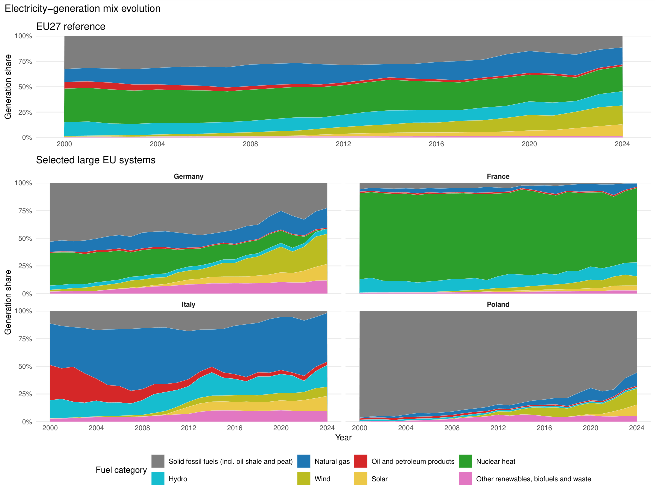
Figure 2.
Fossil–nuclear–renewables ternary trajectories by primary trajectory cluster. Thick colored lines show 3-year moving cluster means for visualization only.
Figure 2.
Fossil–nuclear–renewables ternary trajectories by primary trajectory cluster. Thick colored lines show 3-year moving cluster means for visualization only.
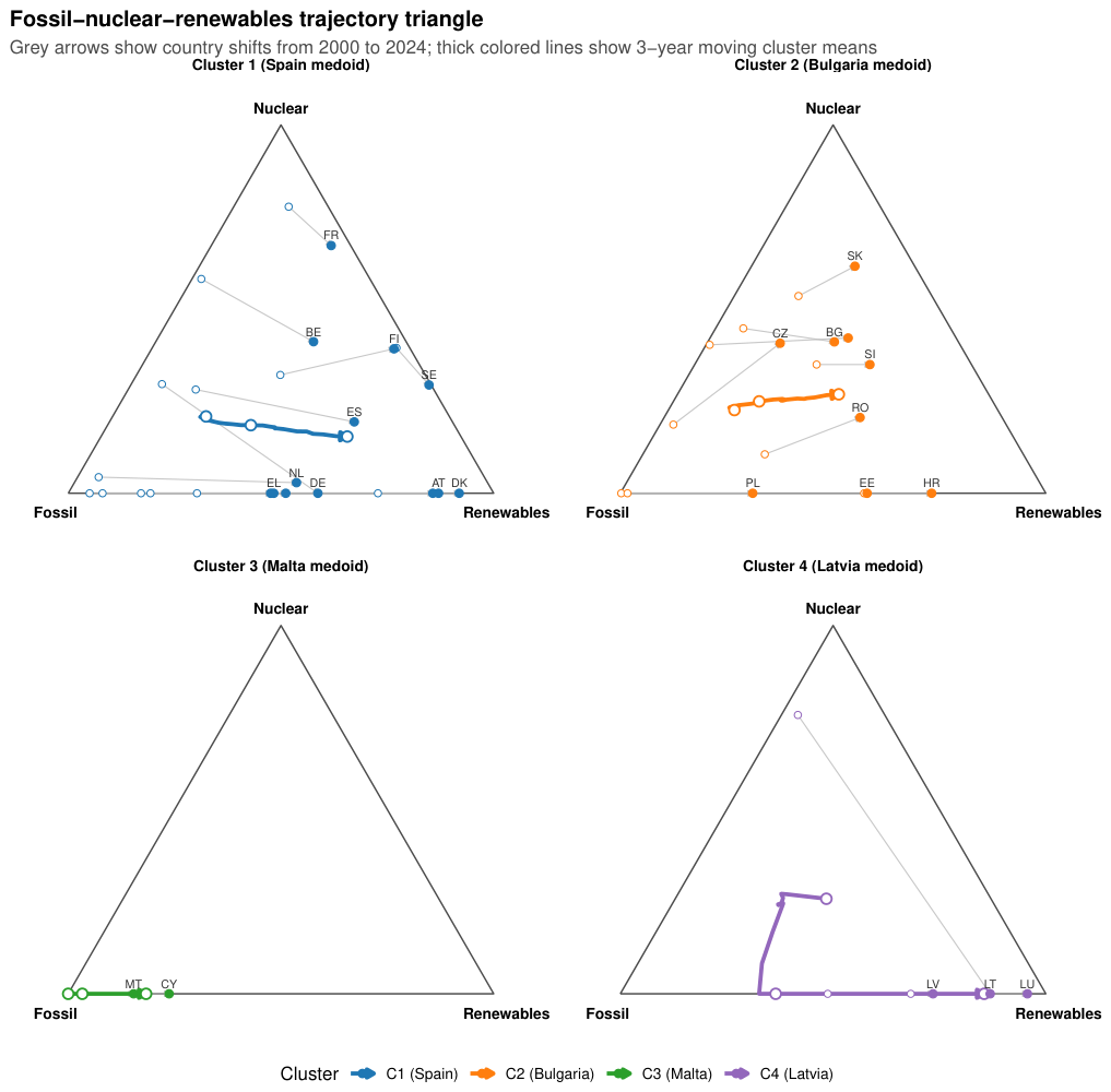
Figure 3.
Mean electricity-generation-mix profiles by primary trajectory cluster.
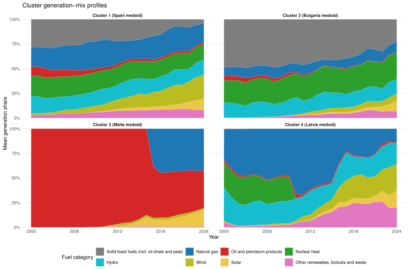
Figure 4.
EU-27 countries by primary compositional trajectory cluster. European countries outside the analytical sample are shown in grey as not analysed; CY and MT identify Cyprus and Malta.
Figure 4.
EU-27 countries by primary compositional trajectory cluster. European countries outside the analytical sample are shown in grey as not analysed; CY and MT identify Cyprus and Malta.
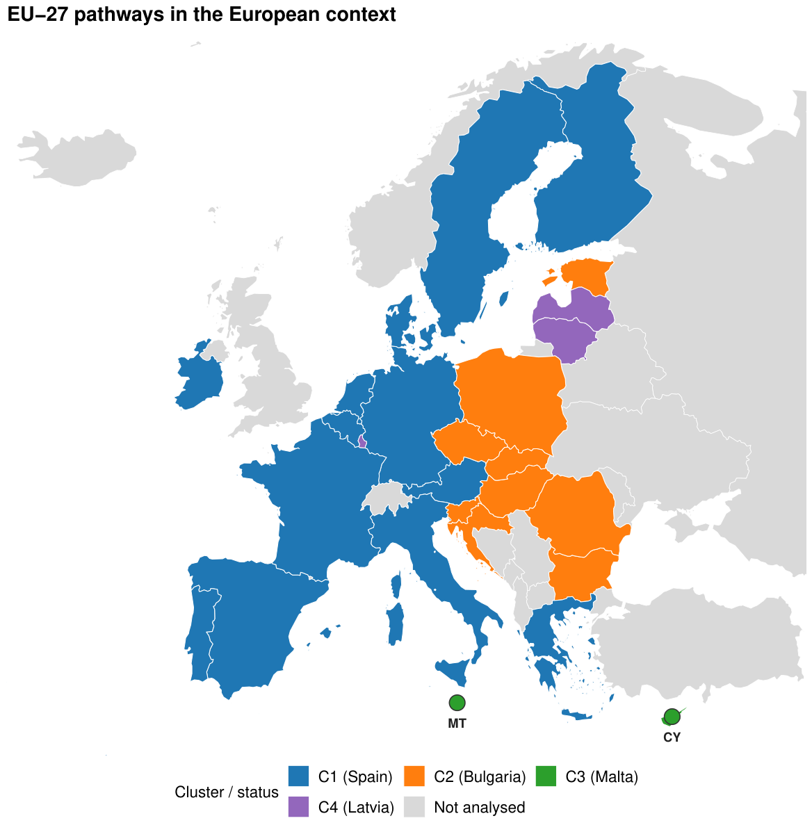
Figure 5.
Within-cluster country trajectories for fossil share, renewables share, and HHI concentration.
Figure 5.
Within-cluster country trajectories for fossil share, renewables share, and HHI concentration.
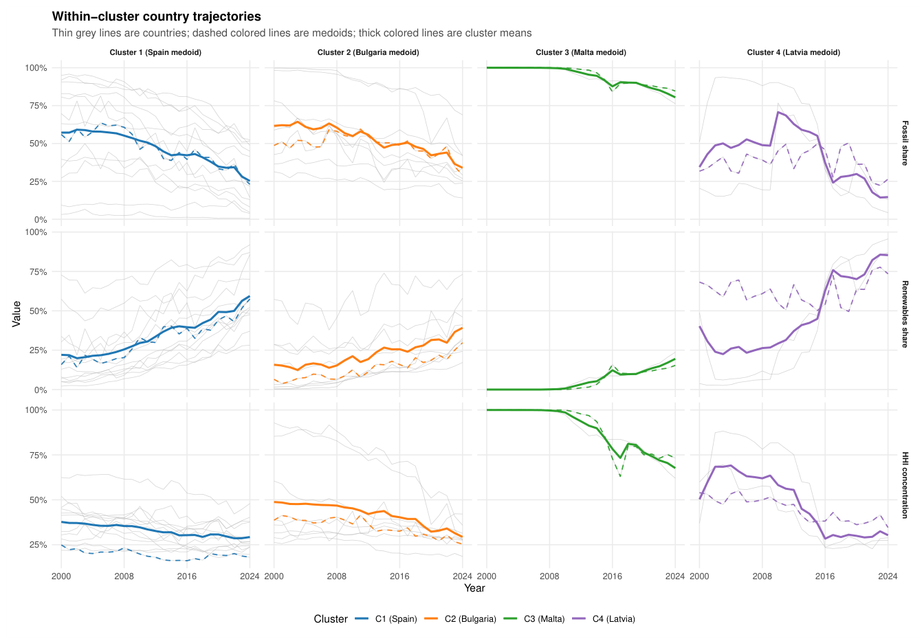
Figure 6.
Validation metrics across candidate values of k. The dashed vertical line marks the selected four-cluster solution.
Figure 6.
Validation metrics across candidate values of k. The dashed vertical line marks the selected four-cluster solution.
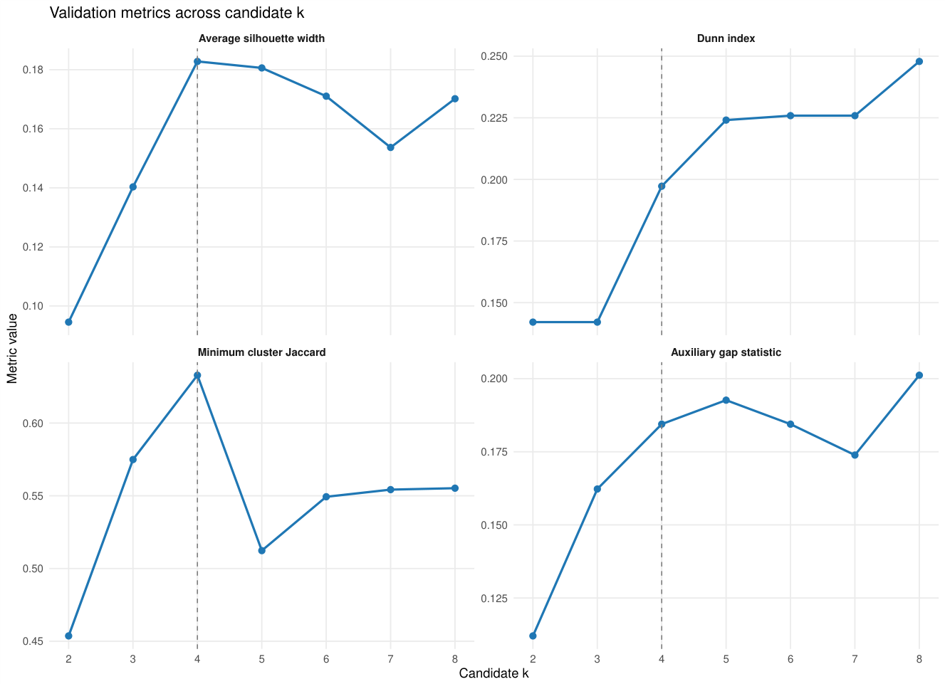
Figure 7.
Country silhouette widths for the primary compositional trajectory clustering. The dashed line marks the overall mean.
Figure 7.
Country silhouette widths for the primary compositional trajectory clustering. The dashed line marks the overall mean.
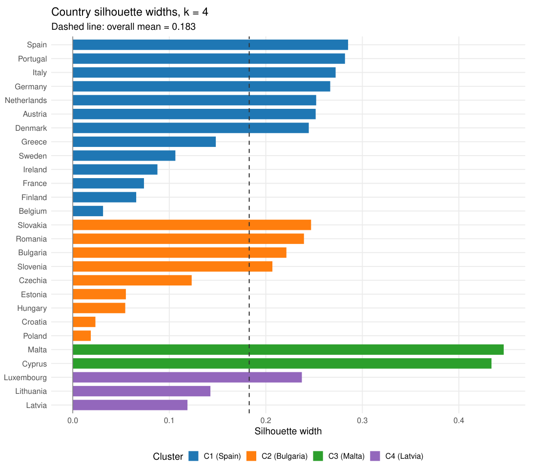
Figure 8.
Adjusted Rand Index across controlled method variants separating representation of the mix from temporal comparison.
Figure 8.
Adjusted Rand Index across controlled method variants separating representation of the mix from temporal comparison.
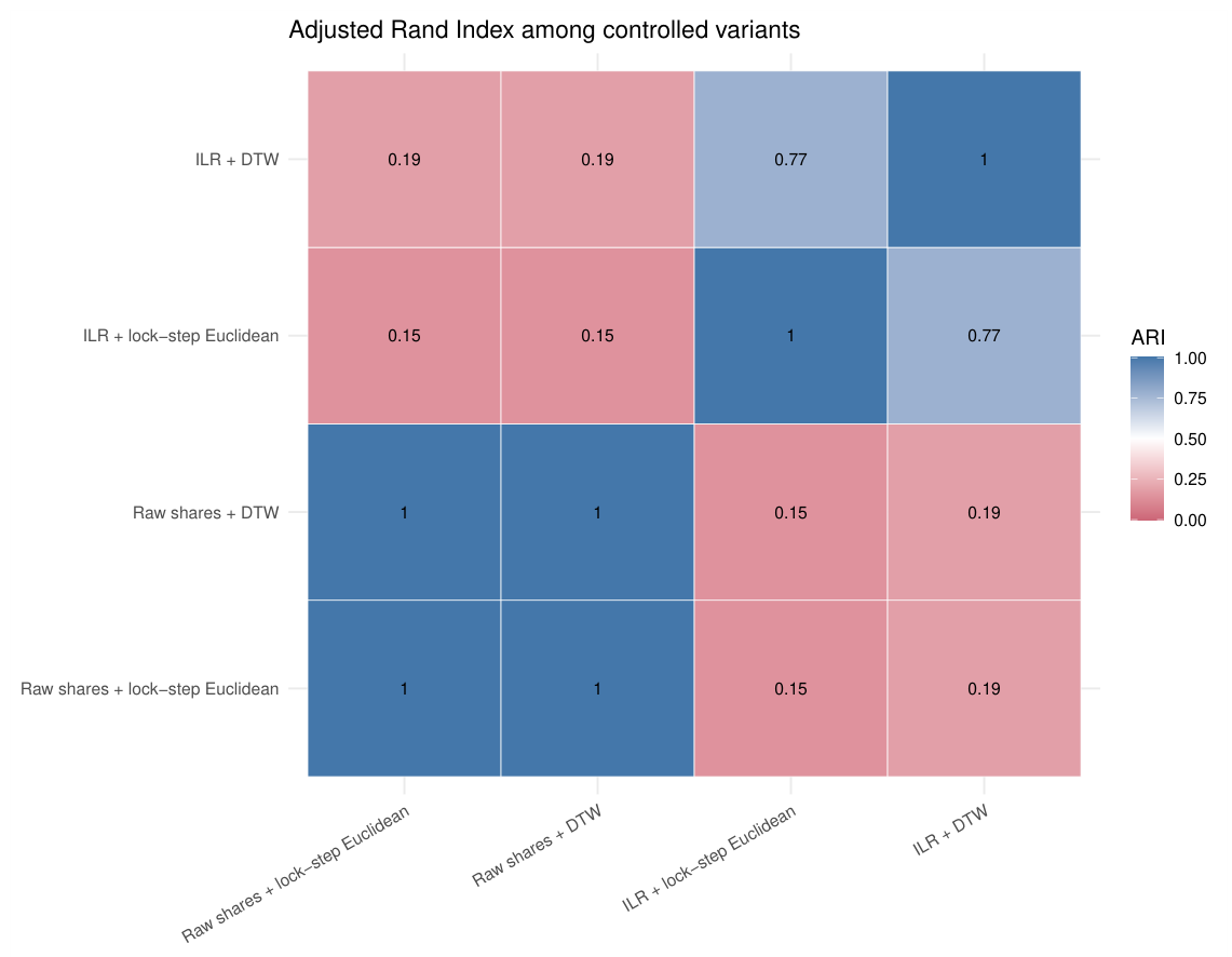
Figure 9.
Endpoint-only similarity versus full-path similarity. Panel A compares pairwise endpoint-distance percentiles in 2024 with full-path distance percentiles for 2000–2024. Panel B shows the crosswalk between endpoint-only clusters and full-trajectory clusters after label alignment.
Figure 9.
Endpoint-only similarity versus full-path similarity. Panel A compares pairwise endpoint-distance percentiles in 2024 with full-path distance percentiles for 2000–2024. Panel B shows the crosswalk between endpoint-only clusters and full-trajectory clusters after label alignment.
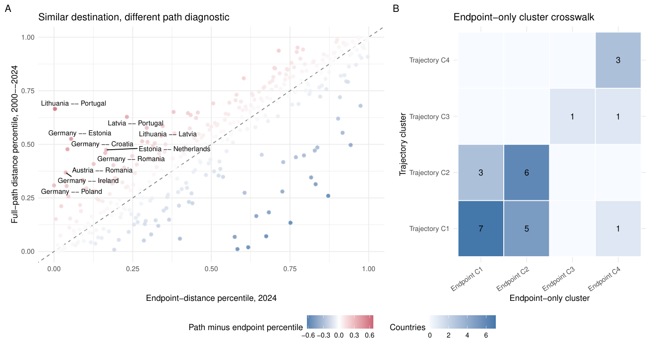
Figure 10.
Cluster-level changes in normalized Shannon diversity and HHI concentration between 2000 and 2024. Open circles show 2000 values, filled circles show 2024 values, and arrows indicate the direction of change.
Figure 10.
Cluster-level changes in normalized Shannon diversity and HHI concentration between 2000 and 2024. Open circles show 2000 values, filled circles show 2024 values, and arrows indicate the direction of change.
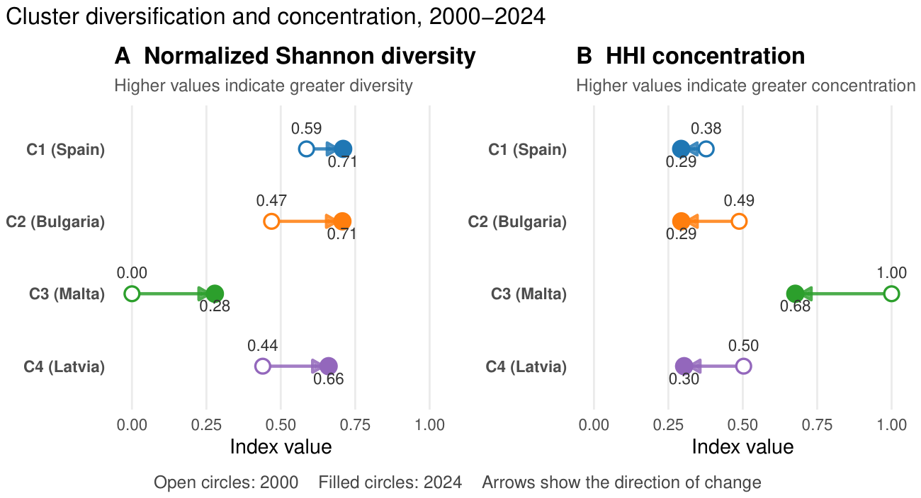
Figure 11.
Concentration-position map based on country HHI in 2024 and HHI change in 2000–2024.
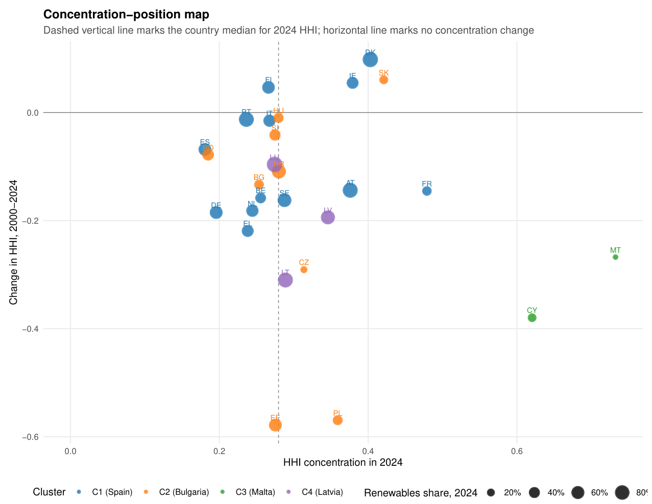

Table 1.
Fuel categories, SIEC codes, and reported-zero diagnostics
| Fuel category | SIEC codes | Aggregation note | Reported zeros | Share of country-years reported zero | Countries zero in all years |
|---|---|---|---|---|---|
| Solid fossil fuels (including oil shale, oil sands, and peat) | C0000X0350-0370, C0350-0370, S2000, P1000 | Includes oil shale, oil sands, peat, and manufactured gases. | 106 | 0.1570 | 3 |
| Natural gas | G3000 | No additional aggregation. | 42 | 0.0622 | 1 |
| Oil and petroleum products | O4000XBIO | Excludes the biofuel portion. | 3 | 0.0044 | 0 |
| Nuclear heat | N900H | Uses the table-specific nuclear code for GEP/GWh. | 341 | 0.5052 | 13 |
| Hydro | RA100 | Excludes pumped hydro (RA130). | 50 | 0.0741 | 2 |
| Wind | RA300 | No additional aggregation. | 53 | 0.0785 | 0 |
| Solar | RA410, RA420 | Combines photovoltaic and thermal solar. | 125 | 0.1852 | 0 |
| Other renewables, biofuels and waste | RA200, RA500, BIOE, W6100_6220, X9900 | Combines geothermal, marine energy, bioenergy, non-renewable waste, and other fuels n.e.c. | 24 | 0.0356 | 0 |
Note: Reported-zero shares use 675 country-year observations per category as the denominator. Raw shares were retained for descriptive indices; simple multiplicative replacement was applied only before ILR transformation.
Table 2.
Cluster composition, medoids and validation metrics
| Cluster | Medoid country | Countries | Mean silhouette | Minimum silhouette | Bootstrap Jaccard | Member countries |
|---|---|---|---|---|---|---|
| C1 | Spain | 13 | 0.1821 | 0.0314 | 0.6940 | Austria, Belgium, Denmark, Finland, France, Germany, Greece, Ireland, Italy, Netherlands, Portugal, Spain, Sweden |
| C2 | Bulgaria | 9 | 0.1321 | 0.0187 | 0.6329 | Bulgaria, Croatia, Czechia, Estonia, Hungary, Poland, Romania, Slovakia, Slovenia |
| C3 | Malta | 2 | 0.4401 | 0.4338 | 0.8833 | Cyprus, Malta |
| C4 | Latvia | 3 | 0.1663 | 0.1188 | 0.8400 | Latvia, Lithuania, Luxembourg |
Table 3.
Concentration and diversification changes by cluster, 2000–2024
| Cluster | Medoid country | Countries | normalized Shannon | HHI 2024 | HHI | effective parts | renewables share |
|---|---|---|---|---|---|---|---|
| C1 | Spain | 13 | 0.1232 | 0.2930 | -0.0840 | 0.78 | 0.3734 |
| C2 | Bulgaria | 9 | 0.2379 | 0.2935 | -0.1944 | 1.10 | 0.2346 |
| C3 | Malta | 2 | 0.2784 | 0.6764 | -0.3236 | 0.49 | 0.1954 |
| C4 | Latvia | 3 | 0.2213 | 0.3030 | -0.1999 | 1.26 | 0.4507 |
Note: Delta values denote the change from 2000 to 2024. Cluster statistics are unweighted means across member countries.
Disclaimer/Publisher’s Note: The statements, opinions and data contained in all publications are solely those of the individual author(s) and contributor(s) and not of MDPI and/or the editor(s). MDPI and/or the editor(s) disclaim responsibility for any injury to people or property resulting from any ideas, methods, instructions or products referred to in the content. |
© 2026 by the authors. Licensee MDPI, Basel, Switzerland. This article is an open access article distributed under the terms and conditions of the Creative Commons Attribution (CC BY) license (http://creativecommons.org/licenses/by/4.0/).
Copyright: This open access article is published under a Creative Commons CC BY 4.0 license, which permit the free download, distribution, and reuse, provided that the author and preprint are cited in any reuse.