

Submitted:
29 September 2026
Posted:
01 October 2026
You are already at the latest version
Abstract
Smart water metering requires low-power, large-scale communication that existing LPWAN solutions do not fully address: the single-hop topology of LoRaWAN needs dense gateway deployments in urban environments, and cellular alternatives incur subscription costs and higher energy consumption. This paper presents a multi-hop LoRa protocol for smart water metering that exploits the static topology and uplink-dominated traffic of this application to simplify the protocol design. Each node selects its relay through a lightweight message exchange and a cost function that combines hop count, relay load and link quality, using only local information, so that the network forms a tree rooted at the gateway. Overhearing the relay retransmission replaces dedicated acknowledgement packets on the relayed hops. The cost function coefficients were tuned by Bayesian optimization for networks of up to 100 nodes, and the best configuration depends on network size. Compared with a shortest-hop (BFS) baseline, the mean peak relay load settles at about 12 clients for 40 to 100 nodes, a reduction of up to 71%, for an average hop-count increase of up to 13%. The transmit energy of the busiest relay falls by up to 69%, although its daily consumption remains dominated by reception. The evaluation covers the topology produced by relay selection and the resulting analytical energy budget.
Keywords:
LoRa
; multi-hop network
; smart water metering
; wireless sensor network (WSN)
; IoT (Internet of Things)
; client load-balancing optimization
1. Introduction
The growing need for efficient monitoring of water resources has driven the adoption of Internet of Things (IoT) solutions in the management of water distribution networks [1]. Smart water meters have emerged in this context as a fundamental tool, enabling remote and automated consumption readings, early leak detection, and more effective management of water infrastructure, with clear advantages over traditional analog meters [2,3]. However, communication between these devices and the central management systems is one of the main technical challenges of their large-scale deployment.
Several wireless communication technologies have been applied in the domain of smart water metering [4]. The first generation of smart water meters adopted short-range protocols such as Wireless M-Bus (wM-Bus), operating in unlicensed spectrum at the 169 or 868 MHz bands in Europe, designed for remote reading systems in which operators equipped with portable receivers collect data in proximity to the meters, in walk-by or drive-by mode. Although this method eliminates the need for direct physical access to the meter, it does not support real-time or automated consumption monitoring. The deployment of fixed gateway networks to address this limitation significantly increases infrastructure costs, making wM-Bus less suitable for large-scale or rural deployments.
LoRaWAN has gained considerable adoption in long-range, low-power IoT applications and is increasingly being used in water metering. Nevertheless, in urban environments, LoRaWAN requires a dense gateway deployment to ensure that indoor devices can successfully transmit data, and its architecture may require subscription costs and dependence on external infrastructures that are not universally available across all regions.
Narrowband IoT (NB-IoT) emerges as a cellular-based alternative operating over licensed networks, offering adequate indoor coverage, however, it requires a subscription to a network operator's service. From an energy consumption perspective, NB-IoT employs synchronous communication using SC-FDMA and OFDMA modulations, which results in higher energy consumption compared to, for instance, LoRaWAN, thereby reducing device battery lifetime [5].
Given these limitations, mesh or multi-hop networks are a promising alternative, as they allow water utilities to deploy and manage their own communication infrastructure without depending on external operators. In these topologies, each node acts both as an end device and as a relay, extending network coverage and reducing the number of gateways required, which directly lowers installation and maintenance costs.
In this context, LoRa (Long Range), the physical layer of LoRaWAN, is well suited to building proprietary mesh or multi-hop networks. Its high receiver sensitivity, low energy consumption and operation in unlicensed frequency bands make it possible to develop communication solutions tailored to smart water meters, with greater flexibility and control over the network.
This article proposes the development and evaluation of a LoRa-based multi-hop network for application in smart water metering, describing the adopted architecture, the proposed protocols, and the results obtained in a simulation environment. The evaluation is confined to the topology produced by the relay selection strategy and to the duty-cycle and energy budgets that follow from it; link-level metrics are outside its scope.
2. Related Work
Extending the coverage of Low-Power Wide-Area Networks (LPWANs) beyond the single-hop star topology imposed by LoRaWAN has been the subject of extensive research in recent years. Since standard LoRaWAN restricts communication to a single hop between an end device and a gateway, coverage gaps caused by obstacles, terrain, or long distances often result in poor connectivity for peripheral nodes. To overcome this limitation, several works have proposed multi-hop and mesh-based extensions to LoRa, which can be broadly grouped into three complementary research directions: (i) routing and protocol design for multi-hop LoRa networks, (ii) relay selection and placement strategies, and (iii) empirical and simulation-based performance evaluations of mesh deployments. This section reviews representative contributions from each of these directions and positions the present work within this body of literature.
Multi-hop Routing Protocols and Network Architectures
A number of studies have proposed dedicated protocols to enable multi-hop communication over the LoRa physical layer while addressing the limitations of the standard LoRaWAN MAC layer. Lundell et al. [6] and subsequent surveys classify these proposals into routing-based approaches, which rely on protocols adapted from ad hoc and mesh networking (e.g., variants of AODV, RPL, and HWMP), and relay-based approaches, in which intermediate nodes perform simple forwarding without maintaining full routing tables.
Mai and Kim [7] proposed a tree-based multi-hop protocol that minimizes end-to-end latency by assigning a dedicated timeslot and channel to each link during a network construction period, exploiting the LoRa capture effect to improve tree-formation reliability. Unlike earlier linear multi-hop schemes, which require a number of timeslots proportional to the number of nodes, this approach enables parallel transmissions across non-interfering branches of the tree, substantially reducing latency while preserving high reliability.
Lee and Ke [8] presented one of the first empirical studies of LoRa-based wireless mesh networking, deploying 19 mesh-enabled nodes over an 800 m × 600 m university campus. Their results showed that the proposed mesh architecture achieved an average packet delivery ratio (PDR) of 88.5%, compared to 58.7% for an equivalent single-hop (star) configuration, demonstrating the practical benefit of multi-hop forwarding in obstructed urban environments without requiring additional gateway infrastructure.
In the context of domain-specific deployments, Marahatta et al. [9] evaluated a LoRa mesh architecture for smart metering in rural microgrids, motivated by the unavailability of reliable cellular or internet infrastructure in remote areas. Their simulation-based analysis, conducted for networks of up to 250 nodes, assessed packet delivery ratio and end-to-end delay as functions of network size and packet size, confirming the feasibility of mesh-based smart metering as a lower-cost alternative to GSM-based systems.
More recently, a LoRaWAN multi-hop device-to-device architecture has been proposed for precision agriculture. The work, targeting smart vineyard monitoring, integrates a digital elevation model, terrain-sensitive propagation effects, and hardware-derived energy profiles into a realistic simulation environment, comparing shortest-path, energy-aware, and learning-based routing strategies for a large-scale (2700+ node) deployment [10]. This study highlights that, in irregular and energy-constrained deployments, routing decisions must jointly account for terrain, residual battery levels, and node mobility to sustain long-term network operation.
Relay Selection and Network Capacity Optimization
A parallel line of research addresses the problem of where and how to select or place relay nodes, rather than the routing protocol itself. Strzoda and Grochla [11] formulated relay selection as a graph optimization problem, in which the network is represented as an undirected graph weighted by the spreading factor required between node pairs. The authors proposed a nature-inspired heuristic, based on Ant Colony Optimization, to select relay locations while explicitly accounting for each device’s energy budget and battery level, a factor often neglected in prior relay-selection studies, which typically rely solely on distance, RSSI or SNR as proxies for link quality. Compared to an exact Edmonds–Karp-based method, the proposed heuristic achieved comparable accuracy (within 2%) at more than twice the computational speed, and consistently outperformed reference methods in preventing premature battery depletion of relay nodes.
Complementary to relay placement, Zhu et al. [12] addressed network capacity through spreading-factor-based clustering. Their Tree-based SF Clustering Algorithm (TSCA) partitions a multi-hop LoRa mesh into several subnetworks, each assigned a distinct spreading factor, thereby exploiting the orthogonality of LoRa chirp signals to enable parallel transmissions. The algorithm balances the airtime across subnetworks while preserving connectivity to the sink node. Its feasibility was confirmed through both simulation and a real multi-floor testbed. This approach illustrates an alternative to conventional relay selection, in which network capacity is improved by reorganizing traffic across the spreading-factor dimension rather than by optimizing individual forwarding paths.
Empirical parent-selection criteria were also investigated by Lee and Ke [8], who analyzed the relationship between RSSI, SNR, and packet delivery ratio in their campus-scale deployment. Their results indicate that stable communication links (PDR > 90%) require RSSI above approximately −110 dBm and SNR above approximately −5 dB, and recommend that nodes avoid selecting parent (relay) nodes below these thresholds, as link reliability degrades sharply and unpredictably in this region.
Discussion and Positioning of the Present Work
Across the reviewed literature, three main strategies for relay selection can be identified: (i) link-quality-based selection, relying on RSSI or SNR thresholds [8]; (ii) energy-aware selection, incorporating residual battery levels and energy budgets into the optimization objective [11]; and (iii) structural or clustering-based selection, in which nodes are grouped according to spreading factor or tree topology rather than through per-node relay assignment [7,12]. While link-quality-based criteria are simple to implement and have been validated empirically, they do not account for the long-term energy sustainability of relay nodes. Conversely, energy-aware approaches such as [11] improve battery-depletion resilience but are typically validated only in simulation, with limited experimental hardware deployment. Structural approaches such as tree-construction [7] and SF-clustering [12] improve throughput and latency but generally assume relatively static network topologies and do not dynamically reassign relay roles in response to changing energy or channel conditions.
This body of work motivates the present study, which combines hop count, relay load and link quality into a single lightweight cost function for distributed relay selection, requiring only local information at each node and relying on a lightweight message exchange for relay discovery. Simulation-based tuning of the cost-function coefficients further shows that the optimal configuration depends on network size.
3. LoRa Overview
LoRa modulation and Gaussian Frequency Shift Keying (GFSK) are the physical layer technologies used for communication between LoRa devices. LoRa employs the Chirp Spread Spectrum (CSS) modulation technique [13], where each transmitted symbol is represented by chirps, with SF denoting the Spreading Factor [14]. Increasing the SF by one step doubles the symbol duration, resulting in a lower data rate but extending communication range and improving receiver sensitivity by approximately 2.5 dB [15,16]. Six spreading factors, ranging from SF7 to SF12, are available. Their quasi-orthogonality allows multiple devices to transmit concurrently on the same frequency channel with limited mutual interference, thereby improving network scalability and spectral efficiency [14].
The reliability of LoRa communications is further improved through Forward Error Correction (FEC), implemented using configurable Coding Rates (CR) between 4/5 and 4/8. Higher coding rates introduce additional redundancy into the transmitted frame, allowing the receiver to recover corrupted bits without requiring retransmissions, at the expense of reduced effective throughput [14,17].
Bandwidth (BW) specifies the frequency span around the carrier frequency that is used for signal transmission, and it indirectly sets how quickly the chirp frequency varies. Higher BW values enable increased data rates, but they come at the cost of reduced receiver sensitivity and a lower link budget. In LoRa deployments, transmissions typically use bandwidths of 125 kHz or 250 kHz [17].
By appropriately selecting SF, BW, and CR, network designers can optimize the balance between communication range, robustness, energy consumption, and data throughput according to the requirements of a given deployment scenario.
LoRa transmissions operate within license-free Industrial, Scientific, and Medical (ISM) frequency bands. Common deployments use 433 MHz, 868 MHz in Europe (regulated under ETSI EN 300 220), and 915 MHz in North America (regulated by FCC Part 15) [9,14,17]. The use of sub-GHz frequencies provides important propagation benefits compared with higher-frequency wireless technologies, including reduced free-space path loss, improved penetration through walls and other obstacles, and enhanced diffraction around obstructions [18]. These properties make LoRa particularly suitable for long-range and non-line-of-sight communications, as well as for indoor deployments where signal attenuation can be significant [19].
In accordance with [13,14], the time-on-air (ToA) of a LoRa packet, , can be calculated as follows:
and can be represented as the sum of the time required to transmit both the preamble and the payload. can be obtained as follows:
where is the number of symbols used in the preamble, typically 8 symbols. is the time of the symbol, in seconds, and can be obtained as follows:
where (Spreading Factor) is an integer parameter ranging from 7 to 12, corresponding to the standard LoRa modulation settings supported by commercial transceivers. Higher values of SF increase communication range and receiver sensitivity at the expense of longer packet transmission times and lower data rates. The bandwidth parameter BW, in Hz, is a discrete configuration value defined by the LoRa physical layer. Typical values are 125 kHz and 250 kHz. Increasing the bandwidth reduces the symbol duration and increases the achievable data rate, while decreasing receiver sensitivity.
The time to transmit the payload can be obtained as follows:
where is the number of symbols to transmit the packet payload and header and is given by:
In Equation (5), indicates the payload length, in bytes. corresponds to the spreading factor, as indicated above. indicates the presence or not of the CRC field ( if it is present, otherwise). indicates the presence or not of the header field ( when the header is enabled, when no header is present). indicates if low data rate optimization is enabled ( when the low data rate optimization is enabled, for disabled). indicates the coding rate ( for 4/5 up to for 4/8).
In LoRa, there are no protocol-level restrictions on the selection of SF and BW combinations. Any limitations that may arise are typically imposed by the hardware implementation of the transceiver.
In contrast, LoRaWAN, the most widely deployed MAC-layer standard built on top of LoRa, defines a set of standardized SF and BW combinations, each associated with a specific Data Rate (DR), which are commonly used in deployed networks. Since the proposed protocol operates directly over the LoRa physical layer and does not implement LoRaWAN, the remainder of this section is included as a contextual reference only. Table 1 summarizes these combinations and their nominal throughput for the EU863-870 band [20].
In these LoRaWAN profiles, the Data Rate (DR) determines both the transmission range and the achievable throughput. Higher DR values increase the throughput. Lower DR values increase communication range by improving receiver sensitivity, while simultaneously reducing the throughput. Figure 1 illustrates this trade-off between data rate and communication range [21].
4. Proposed Work
1.1. System Requirements and Design Assumptions
The development of the proposed LoRa-based multi-hop network is guided by a set of functional and non-functional requirements tailored to the constraints of smart water metering systems, particularly in low-power and large-scale deployment scenarios.
The network shall support multi-hop communication, enabling extended coverage while constraining latency and protocol complexity. Bidirectional communication between nodes and the gateway shall be supported, enabling both uplink data reporting and downlink control or configuration messages, following an uplink-initiated scheme, in which the gateway only transmits in response to a communication initiated by a meter.
Packet retry mechanisms must be implemented to improve reliability in the presence of link degradation or intermittent connectivity. The network shall exhibit resilience to node failures ensuring that alternative paths can be established without requiring manual intervention.
Communication is constrained to occur only between individual meters and the gateway. Peer-to-peer communication between meters is limited to packet forwarding and no direct message exchange between meters is considered.
The system assumes a static network topology, where smart meters are fixed in location. Topological changes are therefore limited to the addition of new nodes or the failure/removal of existing ones, significantly simplifying routing dynamics and network management.
Energy efficiency is also a key design consideration. Both processing overhead and transmission activity shall be minimized in order to prolong battery lifetime, which is a critical constraint in water metering applications. In this context, the protocol design shall avoid unnecessary signaling and reduce radio duty cycle usage.
The solution shall maintain a minimal memory footprint and low computational complexity, ensuring suitability for resource-constrained embedded devices. This includes optimizing code size and reducing processing time per communication cycle.
1.2. Stack Architecture
The proposed protocol follows the layered model illustrated in Figure 2. It operates directly on top of the LoRa physical layer and exposes to the application layer of the metering device a single interface for the exchange of data with the gateway. All addressing, forwarding, relay selection, and integrity verification described in the following sections are implemented within this layer, whose internal decomposition is an implementation concern and is not further detailed here.
1.3. Messages
In the proposed multi-hop network, three types of messages were defined: uplink messages, originated from a node (meter) with the gateway as the destination; downlink messages, transmitted by the gateway as a response, addressed to a specific node and broadcast messages, propagated in all directions across the network, without a single specific destination.
Messages are exchanged exclusively between the meter (end device) and the gateway, in both directions. Direct communication between meters is not supported. Exceptions to this rule occur in two cases:
- When a message is forwarded to another meter (relay node) for retransmission.
- When performing neighbor discovery procedures. In this case a broadcast message is used.
The message is encapsulated within the LoRa PHY payload and is composed of the following fields:
- MAC Header: Contains control information required for message propagation across the network.
- MAC Payload: Carries the transmitted data. This may correspond to application-layer messages or network management messages (services).
- Message Integrity Code (MIC): Ensures message integrity and authenticates that the message originates from the network.
As shown in Figure 3, the fixed protocol overhead comprises the 10-byte MAC Header — encoding relay-level routing information, sequence and retransmission counters, control flags and time-synchronization information (reduced timestamp and synchronization age) — the 3-byte Message Header, carrying end-device identification and message demultiplexing information used by the application layer, and the 4-byte Message Integrity Code, for a total of 17 bytes and leaving up to 238 bytes available for application data out of the maximum 255-byte LoRa PHY payload. The MIC is computed with AES-CMAC [22] over the entire frame, using a network-wide key configured at commissioning. Confidentiality of the meter data, where required, is provided end-to-end by the application layer and is transparent to the multi-hop layer.
1.4. Path Selection Mechanism
To satisfy the requirements of low complexity, reduced energy consumption, and minimal processing overhead, a lightweight routing mechanism is proposed. This approach eliminates the need for nodes to maintain global network knowledge or complete routing tables. In the proposed architecture, each node retains only information about its immediate relay, rather than storing the full path to the gateway. Forwarding responsibility is thereby delegated through a distributed trust model, in which each node relies on its selected relay to propagate messages toward the gateway.
1.1.1. Relay Discovery and Selection
When a node needs to establish or update its path to the gateway, it initiates a local discovery process. This procedure can be triggered under the following conditions:
- initial deployment of the smart meter (node);
- loss of connectivity with the current relay;
- periodic execution, at a low rate configured at commissioning (e.g., once a month), to adapt to network changes such as the addition of new smart meters; a higher rate lets the topology adapt faster, at the cost of additional discovery traffic.
The discovery mechanism is based on a lightweight message exchange (Figure 4), conducted as follows:
- The node broadcasts a WHOS_THERE message to its neighbors (hops = 1).
- Neighboring nodes that are part of a valid path to the gateway and do not have the node as their relay, respond with a HELLO message containing relevant routing metrics, after a random delay to mitigate collisions.
- The node evaluates all received responses and selects the most suitable relay according to the cost metric described below.
- The node broadcasts a RELAY_UPDATE message to inform its neighbors of the selected relay. This message is optional and may be omitted to reduce power consumption, as the neighbors update the internal routing table upon the following messages from the node.
1.1.2. Path Cost Metric
Relay selection is governed by a cost function designed to promote balanced load distribution and prevent traffic concentration on individual nodes. The total path cost is expressed as:
where:
- represents the local link cost to the candidate relay;
- represents the accumulated cost from the candidate relay to the GW, as advertised in the HELLO message;
represents the weight factor between accumulated path cost and local link cost.
The local link cost is formulated as:
where:
- is the number of nodes (direct and indirect) currently served by the candidate relay;
- is a constant used as client load saturation coefficient;
- [dB] is the signal-to-noise value of the candidate relay received message;
- is the maximum signal-to-noise value for actual hardware;
- is the minimum signal-to-noise value of a signal that can be demodulated at any SF;
- are tunable weighting coefficients representing respectively hop count weight, client load weight and link quality weight.
By propagating accumulated cost information through HELLO messages, nodes can make locally optimal relay selections without requiring global topology awareness.
1.1.3. Relay Selection Procedure
The pseudo-codes presented below describe the steps involved in neighbor node discovery and in the selection of a new relay node, based on the mechanisms described in the preceding subsections.
| Algorithm 1 Procedure to initiate neighbor node discovery in order to select a new route to the gateway or update an existing one. This procedure is triggered according to the mechanism described in Section 4.4.1. | ||
| 1: | function SEARCH_RELAY() | |
| 2: | if a new relay search is needed | |
| 3: | - initialize variables | |
| 4: | ||
| 5: | broadcast WHOS_THERE message | - broadcast message with 1 hop |
| 6: | return | |
| Algorithm 2 Procedure to calculate path cost if using node n as relay. Called for each HELLO message received. | ||
| 1: | function PROCESS_HELLO_MSG() | |
| 2: | if node exist on our routing table | |
| 3: | ignore | - ignore, prevents loop paths |
| 4: | else | |
| 5: | calculate using Equation (7) | - link cost to node n |
| 6: | calculate using Equation (6) | - total path cost to gateway |
| 7: | if | |
| 8: | - new cost is better, store it | |
| 9: | - node hops plus 1 | |
| 10: | - store node relay candidate ID | |
| 11: | return | |
| Algorithm 3 Procedure to select the new relay. After a predefined time without responses, the new relay, if any, is selected. | ||
| 1: | function UPDATE_RELAY() | |
| 2: | if timeout waiting for responses | |
| 3: | if and ) | - relative margin to prevent flapping |
| 4: | update with values from new relay | - store new path info |
| 5: | broadcast RELAY_UPDATE message | - informs the neighbors (optional) |
| 6: | else | |
| 7: | Set flag no_relay_valid | - if no relay found |
| 8: | return | |
The pseudo-code presented below describes the steps performed by the neighbors after receiving the WHOS_THERE message in Algorithm 4.
| Algorithm 4 Procedure performed by all neighbors after receiving WHOS_THERE message. | ||
| 1: | function PROCESS_WHOS_THERE_MSG() | |
| 2: | if is our relay or no path to GW | |
| 3: | ignore | - ignore to prevent loops |
| 4: | else | |
| 5: | Broadcast HELLO message with | - reply with its own info |
| 6: | return | |
1.5. Routing Protocol
After a node selects its relay, that relay is used to forward all the uplink messages to the gateway and to receive downlink responses when applicable.
When a node receives an uplink message, it automatically retransmits it using its own selected relay, as direct node-to-node communication is not supported. This process is repeated hop-by-hop until the message reaches the gateway. At each hop, the relay node creates or updates an entry in its routing table corresponding to the originating node. This way, each node maintains a local routing table of downstream nodes for which it currently acts as relay, enabling management of the downlink messages for its clients.
When a node receives a downlink message, it first checks whether it is the intended destination. If so, the message is processed locally; otherwise, it is forwarded to the next node along the reverse path, using the routing information previously stored in the routing table.
To prevent routing table overflow, each entry is associated with a Time-To-Live (TTL) value. Entries corresponding to nodes with no activity exceeding the TTL are automatically removed from the routing table.
Each message carries a sequence counter assigned by the originating node and conveyed within the MAC header, together with a retransmission counter. A relay records the highest sequence counter received from each source and uses it to recognize messages it has already forwarded, which prevents a broadcast message from being propagated more than once when it reaches a node through multiple paths, and rejects the replay of previously captured messages. A retry repeats the sequence counter of the original message and is distinguished from a replay by the retransmission counter. The relay retransmits it so that the originating node can detect it, even though the next hop discards it as already received. Since the MIC also covers the reduced timestamp that every frame carries, a device without the network key can neither forge nor alter a message, and a node discards any frame whose timestamp does not fall within the current operation window, the scheduled interval in which the network is active. This protects discovery against HELLO messages replayed from earlier windows, including at a newly installed node that has no counter history, and prevents a device outside the network from attracting traffic with a false low-cost advertisement.
The protocol does not employ explicit acknowledgement packets to confirm message reception. Instead, upon transmitting or retransmitting a packet, a node remains in listening mode until it overhears its relay retransmitting that same packet, implicitly confirming successful reception. The gateway, being the final destination, does not forward the message. Instead, upon receiving an uplink message it transmits a header-only copy, without application payload, which gives the last relay the same implicit confirmation as any other node on the path at a small fraction of the airtime of a full retransmission. This approach dispenses with dedicated acknowledgement packets on the relayed hops and confirms that the relay has forwarded the message, and not merely received it (Figure 5).
If the listening window expires without detecting the expected retransmission, the node retries the transmission up to two additional times. Should all three attempts fail, the node concludes that its relay is no longer reachable and schedules a new relay discovery process to establish an alternative path to the gateway.
With this architecture, the path between a node and the gateway is implicitly established and maintained through the periodic transmission of uplink messages. Consequently, the gateway can only reach a meter after that meter has transmitted: an on-demand request issued by the head-end system is held by the gateway and forwarded along the reverse path when the meter reports in its next operation window, which must then also accommodate the downlink exchange, so that its latency is bounded by the reporting period. Configuration messages follow the same mechanism, and those addressed to all meters can use the broadcast message type of Section 4.3.
1.6. Energy Consumption Reduction Mechanisms
Commercial smart meters are commonly available with energy consumption logging resolutions of 15, 30, or 60 minutes, with 15-minute intervals among the most frequently offered configurations. These high-resolution profiles enable fine-grained load analysis and billing accuracy; however, when transmitted over low-power wide-area networks (LPWANs) such as LoRa, the communication overhead associated with frequent transmissions can represent a significant fraction of the total energy budget of a battery-operated metering node.
To address this constraint, it is advisable to aggregate as many consecutive measurements as possible into a single transmission frame, exploiting the maximum LoRa physical layer payload size of 255 bytes. This approach reduces the effective energy consumption per payload byte by amortizing the fixed overhead of the radio preamble, PHY header, and MAC layer fields across a larger data block [24]. From an information-theoretic perspective, this is equivalent to improving the transmission efficiency by increasing the ratio of application data to protocol overhead. Given a 15-minute measurement resolution and a compact encoding scheme, for instance, representing each consumption sample as a 2-byte value, a full day of readings (96 samples) amounts to 192 bytes which, together with the 17-byte protocol overhead, yields a 209-byte LoRa PHY payload, well within the 255-byte maximum available at any spreading factor, and reduces the reporting activity to a single daily transmission.
Building upon this aggregation strategy, it is further possible to define scheduled operation windows during which the network is active and end devices transmit their buffered data to the gateway. Outside these windows, radio transceivers can be placed in a low-power sleep state or fully powered down, depending on the hardware capabilities of the end device. This duty-cycled operation is well-established in the LPWAN literature as one of the most effective techniques for extending node lifetime in energy-constrained deployments [25,26]. The combination of payload aggregation and scheduled transmission windows allows the system to decouple the measurement sampling rate from the transmission rate, a design principle that is particularly relevant in metering applications where real-time delivery is not required and data can be buffered locally in non-volatile memory.
The duration of each operation window must be dimensioned to accommodate all expected packet transmissions under normal network operation, and can be obtained as follows:
where:
- is the maximum nodes expected for the network;
- is the maximum hops expected for the network;
- is the maximum packet time-on-air supported by the network according to Equation (1).
Equation (8) dimensions the window as max_nodes intervals of max_hops × ToA_max, each long enough for one report to reach the gateway along the deepest path. The window can therefore be operated as a schedule of max_nodes slots, one per end device and assigned at commissioning, so that systematic contention between end devices is avoided by construction rather than resolved at the medium access level. Enforcing the slot boundaries is a function of the application layer of the metering device; the stack performs a channel activity detection before each transmission as a safeguard against external interference.
In addition to accommodating all transmissions, the operation window must comply with the regional duty-cycle regulations (1% per device in the EU 868 MHz sub-bands under ETSI EN 300 220 [27]). The airtime of the most loaded relay must not exceed 1% of the regulatory observation period. This constrains the combinations of spreading factor, payload size, and window periodicity available to the network planner.
The schedule of the operation windows is anchored to fixed times of day and is configured at commissioning time together with the remaining device parameters; the time of day itself is maintained by the gateway, which has access to a real-time reference. Because the relay discovery exchange of Section 4.4.1 takes place within this window, neighboring nodes are listening by construction and no dedicated wake-up mechanism is required.
The slot schedule requires the nodes to share a common time-of-day reference. Rather than distributing it through a dedicated broadcast, which in a multi-hop network would have to be re-flooded tier by tier and would add unacknowledged, collision-prone traffic to every window [17], the reference is piggybacked on existing traffic. Every frame, including the header-only confirmation issued by the gateway, carries a reduced timestamp (the sender’s time of day with sub-second resolution, captured at the start of transmission) and a synchronization age, which counts the operation windows elapsed since that value was last traceable to the gateway. A node receiving a frame from its relay recovers the transmission start by subtracting the time-on-air of the received frame (Equations (1)–(5)) from its reception timestamp [7], and adopts the sender’s time whenever the sender’s age does not exceed its own. Since the radio remains in reception throughout the window, this applies to every transmission of the relay and not only to the retransmission that serves as implicit acknowledgement, so that a node may be updated several times within a window, always towards a fresher reference. No additional messages or listening time are required, and a missed update is recovered by the same retry and relay rediscovery procedures that protect data delivery. The initial time is set at commissioning.
Because a relay forwards a frame before overhearing the onward retransmission, a fresh reference reaches the deeper nodes only through subsequent transmissions of their relays, and whether it reaches all of them within the same window depends on the slot order, which bears no relation to the position of the nodes in the tree. A node may therefore close a window with a reference that is one or more windows old. The synchronization age makes this condition known to the node and to its relay, and the guard interval is dimensioned as Tguard [s] = 2 × (1 + a) × δ × Tw, where δ is the oscillator tolerance (dimensionless, 30 × 10−6 for ±30 ppm), Tw is the window period in seconds and a is the largest synchronization age, in windows, among the node and its clients at the end of the previous window. For an uncompensated 32.768 kHz oscillator with a tolerance in the order of ±30 ppm, each node accumulates up to ±2.6 s of drift over a daily period, giving a guard interval of 5.2 s for nodes refreshed in every window (a = 0), which is the normal condition. The daily radio active time of a node is therefore given by:
where is obtained from Equation (8) and is the guard interval.
5. Materials and Methods
The performance evaluation was carried out with a purpose-built, discrete-cycle simulator that models the network formation process described in Section 4.4. The LoRa physical and MAC layers are not modeled: the simulator operates at the routing level, so the evaluation characterizes the topological properties of the relay selection strategy (hop count, relay load, and convergence speed). The per-node energy consumption is not measured by the simulator either, but derived analytically from the resulting topology.
Each topology places a single gateway and 10 to 100 nodes over a square area of 800 × 800 pixels, with a node coverage radius of 150 pixels, using a farthest-point random placement in which every new node is positioned within radio range of a previously placed one; the generated topologies are therefore connected by construction, reflecting the practical requirement that a deployed meter must be within range of at least one other network element. Two nodes can communicate if and only if the distance between them does not exceed the coverage radius, and the link SNR used in Equation (7) is obtained by linearly mapping the inter-node distance from [0,150] pixels onto [+30, −20] dB. The upper bound of +30 dB corresponds to the term already introduced in Equation (7). The lower bound of −20 dB is taken from Table 2 and corresponds to the most permissive demodulation threshold available in the radio, obtained at SF12; it is applied as a single, SF-independent floor, since spreading factor adaptation is not modeled. This mapping is not intended as a propagation model: the relay selection operates on the SNR reported by the radio, irrespective of the physical mechanisms that produced it, and the simulator only requires a plausible spread of link qualities across the neighborhood, which the distance mapping provides while remaining directly representable in the topology plots. Distances are expressed in pixels, a dimensionless unit: relay selection depends only on the position of the nodes relative to the coverage radius, so no physical scale is implied. The remaining constants were set to K_cls = 10 and a relay-switching hysteresis margin of 5% of the current path cost.
The simulators were implemented in Python 3.13.3, using Microsoft Visual Studio Code 1.128.0 as the development environment. The source code was developed with the assistance of Claude Sonnet 5 (Anthropic), which was used to generate code from specifications defined by the authors. All generated code was reviewed, validated, and tested by the authors. All simulations were carried out on a FUJITSU Server PRIMERGY RX2510 M2 with two Intel® Xeon® E5-2620 v4 processors and 64 GB of memory.
6. Performance Evaluation
1.1. Graphical Simulator
To evaluate the effectiveness of the proposed relay selection strategy, a dedicated simulation environment was developed. The simulator models the network formation process from an initial set of nodes, allowing systematic analysis of how different parameter configurations affect path selection and the resulting network topology. Specifically, it enables observation of how variations in the weighting coefficients of the cost function, together with link-related metrics such as SNR margin and hop count, influence route distribution, load balancing across relay nodes, and the stability of established paths over time. The simulator executes the relay selection algorithm of Section 4.4 in discrete cycles on a static map of node positions, each cycle corresponding to one round of relay discovery in which every node updates its relay (Section 4.4.1); this mirrors the periodic verification of the topology in a deployed network.
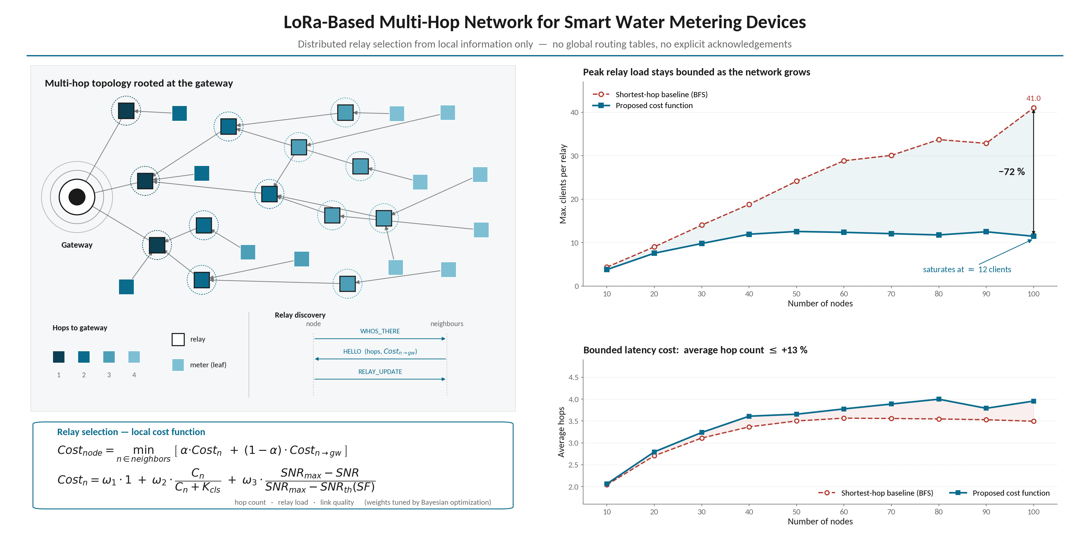
Figure 6 shows a snapshot of the Best Path Finding Algorithm Simulator, illustrating the resulting multi-hop topology for a given parameter configuration.
The simulation results provide insight into the algorithm's behavior under changes of the network parameters, supporting the identification of parameter sets that yield a more uniform and efficient topology. In addition to numerical output, the tool provides visual inspection of the resulting network structure, which facilitates qualitative validation of the intended load distribution properties and helps identify undesirable patterns—such as relay bottlenecks or isolated branches—that may not be immediately apparent from aggregate metrics alone.
This evaluation showed that multiple combinations of coefficients can lead to satisfactory network behavior, while others result in unstable topologies, characterized by frequent relay changes and uneven load distribution.
1.2. Parameter Optimization
Although the graphical simulator described above proved useful for visually inspecting the resulting network topology and validating the load distribution qualitatively, it does not provide a systematic way to find the best set of weighting coefficients, particularly across different network sizes. To address this, a second simulation framework was developed using the Optuna hyperparameter optimization library [28] to automate the search for the best parameter values. This approach treats parameter selection as an optimization problem, where each trial is a candidate set of weighting coefficients evaluated against an objective function that reflects the desired network properties. Optuna's sampling algorithm, the Tree-structured Parzen Estimator (TPE) [29], explores the parameter space step by step, using the results of previous trials to guide the search towards more promising regions, rather than using an exhaustive or random search.
The objective function combines two network metrics, computed over a set of 30 fixed node distributions, for each network size tested: the average number of hops between a node and the gateway (avg_hops) and the average of the load on the most overloaded relay (avg_max_clients) in each topology, that is, the peak number of clients served by a single relay and not the average number of clients per relay across the network. This second choice is not arbitrary: an earlier version of the objective function used the average number of clients per relay (avg_clients) as the load-balancing term, and it turned out that the optimizer then converges to a shortest-hop tree, as built by Breadth-First Search (BFS). Across the full range of network sizes tested, the optimizer using avg_clients as the load term consistently converges to an avg_hops (Figure 7a) that matches the BFS reference almost exactly, for every network size evaluated. This happens because avg_clients is largely blind to how load is spread across relays: a tree with a single heavily overloaded relay and many almost idle leaf nodes can still show a low average, so the optimizer has no reason to accept longer paths, at any of the network sizes tested.
In contrast, using the maximum clients (max_clients) directly as the load term, which penalizes having an overloaded relay instead of hiding it in a network-wide average, results in a slight increase in avg_hops relative to BFS, ranging from about 3% at 20 nodes to around 13% for the larger networks (Figure 7a). This small penalty is, however, largely compensated by the gains in load balancing: the reduction in avg_max_clients compared to BFS grows markedly with network size, from around 16% at 20 nodes up to 71% at 100 nodes (Figure 7b), showing that the benefit of directly penalizing the most overloaded relay becomes increasingly significant as the network grows and load concentration becomes a more pressing issue. It was this difference in behavior that led to adopting max_clients as the load metric in the objective function.
Before the TPE search itself, a calibration phase is performed in which 300 samples are generated using Latin Hypercube Sampling [30] over the parameter space [α, ω1, ω2, ω3] ∈ [0,1]⁴. This ensures a more uniform coverage of each parameter range than simple random sampling. Each of these 300 candidate combinations is evaluated over the same 30 fixed topologies, and the minimum and maximum values of avg_hops and avg_max_clients observed among the qualifying combinations are used to normalize (min-max scaling) both metrics onto a comparable [0,1] scale, before combining them by a simple sum into the final objective function that the TPE search minimizes. A combination of coefficients is only considered qualified if it manages to connect every node to the gateway in all 30 topologies tested.
To verify that the result does not hinge on the equal weighting of the two normalized terms, or on the calibration sample that sets their ranges, every qualified configuration evaluated by the TPE search (more than 1200 per network size) was placed in the (avg_hops, avg_max_clients) plane. At every network size tested, the selected configuration lies on the Pareto front, i.e., no evaluated configuration achieves both fewer hops and a lower peak load, and it scores better than the BFS reference unless the hop term is weighted more than about six times the load term.
This optimization process was repeated for several network sizes, in order to check whether the best parameter configuration stays stable as the number of nodes grows, or whether it has to be adapted to the scale of the network.
Figure 8 shows the values of α, ω1, ω2 and ω3 obtained across the different optimization runs, plotted as a function of the number of nodes in the network. This lets us spot trends in how each coefficient changes with network size, and show that the best parameter values are not invariant with respect to network size, although the pattern differs from coefficient to coefficient.
The load balancing weight, ω2, remains consistently the dominant term across the entire range tested, staying between 0.80 and 1.00 from 20 nodes onward, which confirms that penalizing the most overloaded relay is the primary driver of the cost function at all the network sizes tested. The link quality weight, ω3, follows the opposite pattern, staying close to zero at every network size tested (at most 0.09) and vanishing entirely at 10, 20, 90 and 100 nodes, which indicates that link quality has little influence on the two metrics optimized here.
The remaining two coefficients, α and ω1, show a size-dependent behavior of their own. For smaller networks, up to 30 nodes, both vary considerably across runs (α between 0.10 and 0.25, ω1 between 0.11 and 0.42), whereas from 40 nodes onward both settle into a narrow, stable range (α between 0.01 and 0.03, ω1 between 0.13 and 0.22). This behavior can be explained by the specific role each of these coefficients plays in the cost function. In Equation (7), ω1 multiplies a fixed unit cost, acting as a constant penalty applied at every hop; since this per-hop cost accumulates along the path to the gateway through the recursive term in Equation (6), its overall contribution to the total path cost scales with the depth of the tree. Similarly, α does not weight one of the individual cost components but instead controls, at every hop, how the local cost is blended with the already accumulated cost of the candidate relay, because this blending is applied recursively at each hop, its effect on the final cost compounds with tree depth rather than adding linearly. In small networks, trees are shallow and the number of hops to the gateway is limited, so both the accumulated effect of ω1 and the recursive composition of α have little room to manifest, resulting in only small differences in total cost between candidate parameter values; the objective function is therefore comparatively insensitive to α and ω1 in this regime, which explains the scattered values obtained by the optimizer. As the network grows and paths to the gateway become longer, the per-hop penalty introduced by ω1 and the compounding effect of α accumulate over more hops, making the objective function increasingly sensitive to both coefficients; the search space consequently develops a well-defined optimum, which is reflected in the stabilization of both parameters from 40 nodes onward. It should be noted that the low values to which α and ω1 converge in large networks do not indicate that these coefficients become irrelevant; rather, because its effect compounds over deeper trees, even small variations produce large differences in total path cost, and the optimizer therefore settles on a precise, deliberately small value that avoids over-penalizing long paths.
This means that a fixed, size-independent parameter configuration is not enough to guarantee good behavior across networks of different scales. While the dominance of the load-balancing term is a robust feature of the optimization across the whole range tested, the relative weight given to path length (ω1) and to the balance between local and accumulated cost (α) only becomes clearly defined above a certain network size, and should be reconsidered, or re-optimized, when deploying the algorithm on networks below that threshold.
1.3. Network Topology
Having established that the optimal parameter selection is network-size dependent, it is worth measuring the real impact of this optimization on network performance by comparing it against a reference baseline: a shortest-hop tree (BFS). This type of tree connects each node to the neighbor offering the shortest path, in hop count, to the gateway, ignoring load distribution across relays entirely. By construction, BFS is the lower bound for the average hop count and shortest-hop trees are adopted as the initial tree construction in multi-hop convergecast schemes [12,31]; BFS is therefore the reference against which the effect of relay load on the resulting topology is measured.
Figure 9 shows the evolution of average hops (avg_hops) for the proposed solution and for the BFS baseline, as a function of the number of nodes. For small networks the two curves are nearly indistinguishable (2.06 against 2.04 at 10 nodes, 2.79 against 2.71 at 20 nodes). As the network grows, the optimized solution deviates from the lower bound, stabilizing around 3.7–4.0 hops against 3.5 for BFS, a worst-case penalty of approximately 0.45 hops or 13%, at 50 nodes and above. This modest cost is the price of routing part of the traffic through longer but less congested paths.
Figure 10 shows the equivalent comparison for average maximum clients (avg_max_clients), and this is where the benefit becomes clear. Under BFS, the peak load per relay grows almost linearly with network size, from 4.4 clients at 10 nodes to 41.0 at 100 nodes, since nodes systematically converge on the few relays closest to the gateway. The proposed solution, in contrast, saturates at roughly 12 clients from 40 nodes onward (11.9 at 40 nodes, 12.0 at 100 nodes), effectively decoupling the peak relay load from the network size within the tested range. The resulting reduction relative to BFS grows with network size, from 13% at 10 nodes and 37% at 40 nodes to 58% at 60 nodes and 71% at 100 nodes. The 95% confidence intervals of the two methods do not overlap for the peak load from 30 nodes onward.
Taken together, Figure 9 and Figure 10 show a highly asymmetric trade-off: a hop-count penalty bounded at approximately 13% buys a peak-load reduction that reaches 71%, and that grows with network size as more nodes compete for the relays near the gateway.
The observed saturation of the peak relay load also has a regulatory benefit. Since the airtime of a relay grows with the number of clients it serves, the fact that the mean peak load settles at approximately 12 clients from 40 nodes onward keeps the most loaded relay, on average, within the ETSI duty-cycle budget under configurations where a BFS tree, whose peak load grows linearly with network size, would exceed it.
As an illustrative example, consider the 209-byte payload of Section 4.6 transmitted at SF10 (125 kHz, CR 4/5), for which Equations (1)-(5) yield a time-on-air of approximately 1.9 s. Since the mean peak relay load settles at approximately 12 clients for networks of 40 nodes or more, the most loaded relay accumulates about 25 s of airtime per operation window, remaining within the 36 s/h allowed by the 1% duty cycle. The limit corresponds to 18 clients per relay at SF10; the peak load of some simulated topologies exceeds it (up to 28 clients), and these require the window splitting described below. Higher spreading factors increase the time-on-air and may exceed this budget. Since the duty-cycle limit applies on an hourly basis, compliance can be restored by splitting the daily report across multiple operation windows scheduled in different hours (at SF11, two windows per day keep the busiest relay near 31 s per window; SF12 remains feasible but requires a substantially larger number of windows, and is therefore advisable only where the link budget requires it). This comes at the cost of a higher aggregate time-on-air, as the fixed per-packet overhead is paid more than once, with a corresponding impact on energy consumption. The example configuration above is used only to verify duty-cycle compliance and does not constrain the spreading factor adopted in the following sections. Under the BFS baseline the same configuration would place the busiest relay at about 80 s per window at 100 nodes, more than twice the regulatory budget. The gateway is subject to the same limit and must confirm every report: a 17-byte header-only frame takes 0.33 s at SF10, so the 36 s/h budget limits a single gateway to 109 nodes per operation window.
Figure 11 shows the distribution of maximum clients (max_clients) per seed, as a box plot, for the optimized solution and for the BFS baseline at five representative network sizes (20 to 100 nodes, in steps of 20, intermediate sizes follow the same trend and are omitted for readability).
It confirms that the reduction in peak load does not come from a small number of particularly favorable topologies, but from a general compression of the distribution. As the network grows, the spread of the proposed solution narrows while that of BFS widens, and from 60 nodes onward the two distributions barely overlap. The clearest case is the 100-node network, where the worst topology served by the proposed solution (17 clients) still outperforms the best one served by BFS (19 clients). The only exception is the 20-node network, where the proposed solution shows a slightly wider spread than BFS; at this size, with few candidate relays available, the optimization trades consistency across topologies for a lower average peak load. In short, for networks of 40 nodes or more, load balancing is not only better on average but also markedly more predictable from topology to topology, which matters for real deployments where the exact position of the nodes is not under control.
Finally, the number of cycles required for the network to form was recorded for the proposed solution at each network size, where a cycle corresponds to one execution of the relay discovery procedure by every node. Two metrics are distinguished: the number of cycles until all nodes obtain a valid path to the gateway, and the number of cycles until the network stabilizes, i.e., no node changes its relay in subsequent cycles. These results correspond to a cold-start scenario, in which the entire network is formed at once from nodes without any established relay. This is a worst-case situation, since in a real deployment the network forms progressively, as new meters are installed and join an already established topology. Figure 12 shows that full connectivity is reached quickly at every scale, taking between 2.4 and 3.9 cycles on average, with no clear dependence on network size. Stabilization takes longer and grows with network size, from 3.7 cycles at 10 nodes to 19.7 cycles at 100 nodes.
Two observations follow. First, the time to connect all nodes is essentially independent of network size: the additional depth of larger trees is compensated by the higher node density, which increases the number of candidate relays and allows more nodes to connect in parallel in each cycle. Second, the growing gap between connection and stabilization reflects the load-balancing behavior of the cost function: the first cycles suffice to connect every node, while the subsequent ones progressively redistribute clients away from overloaded relays until an equilibrium is reached. Even in this worst-case cold-start scenario, stabilization time remains modest, staying below 20 cycles across a tenfold increase in network size.
1.4. Energy Analysis
This section evaluates the energy performance of the nodes as distributed by the proposed algorithm. Since every relay must forward the traffic of all the clients it serves in addition to reporting its own readings, the node holding the largest number of clients is the one subjected to the highest transmission and reception activity, and therefore is the most energy-critical point of the network. The analysis consequently focuses on this worst-case node. The nodes are assumed to be active only during a bounded daily interval, the operation window, and to remain in a low-power state for the rest of the day; the duration of this window is obtained from Equation (8) for each network size, taking max_hops as the mean, over the 30 topologies, of the maximum hop count of each tree. The charge drawn by the busiest node over one day is then estimated with Equation (10),
where:
- is number of clients of a given node;
- is the packet time-on-air supported by the network according to Equation (1), converted to hours;
- is the daily radio active time according to Equation (9), converted to hours;
- [A] is the current consumption of the radio in TX mode;
- [A] is the current consumption of the radio in RX mode;
- [A] is the current consumption of the radio in OFF mode.
During the operation window the node transmits its own reading plus one retransmission for each of its clients, so the total transmit time is (. Outside these transmissions the radio is kept in reception for the remainder of the window, and it is placed in the low-power OFF mode for the rest of the day. Relay discovery is not included in Equation (10): it takes place within the operation window, whose reception time is already accounted for, and its short messages, exchanged at installation, after a relay loss or at the low periodic rate of Section 4.4.1, add a negligible transmission time when amortized over the days between executions. The corresponding daily energy is obtained from Equation (11),
where:
- is the electric charge given by Equation (10);
- [V] is the battery supply voltage.
The time-on-air was computed for the 209-byte payload of Section 4.6 using a raw-LoRa configuration (SF = 9, BW = 125 kHz, CR = 4/5) with an explicit header, no CRC and an 8-symbol preamble, yielding approximately 1.05 s. SF9 offers a good balance between range and time-on-air, and is adopted here as a realistic operating point for the energy estimates that follow. The guard interval of Section 4.6, 5.2 s for nodes refreshed in every window (a = 0), is rounded up to 6 s.
The radio currents correspond to the Semtech SX1261 transceiver [32], with at +14 dBm output power, and , operating from a 3.3 V supply. The results are presented alongside those of a BFS reference network built on the same topologies.
Figure 13 shows the resulting daily radio active time as a function of the number of nodes. The two windows are nearly identical at 10 nodes, and for larger networks the window of the proposed algorithm is longer, by up to about 23% at 100 nodes (880 s versus 716 s). This follows directly from Equation (8), in which the window is proportional to the maximum hop count: the load-balanced trees produced by the proposed algorithm are deeper than the shortest-hop BFS trees and therefore require a longer window to accommodate all forwarded transmissions.
Figure 14 reports the daily energy of the busiest node, the most critical point of the network in terms of consumption, split into the transmission (TX) and reception (RX) terms of Equation (10). The relay load is the average, over the 30 topologies, of the maximum client count (max_clients) at each network size.
The transmission energy is where the proposed algorithm stands out. Since the busiest node transmits its own report plus one retransmission per client, the TX term follows the peak relay load of Section 6.3: it remains at about 0.32 mWh per day from 40 nodes onward, whereas under BFS it keeps growing with network size, up to 1.03 mWh at 100 nodes, a reduction of 69%. The total daily energy, however, is similar for both methods, with differences within ±5% across the tested range (3.98 mWh versus 3.87 mWh at 100 nodes).
The reason lies in the structure of the energy budget. The operation window is dimensioned from Equation (8) as a function of the maximum hop count and the network size, and is therefore independent of how the clients are distributed among the relays: every node keeps its radio active for the whole window and spends the fraction not used for transmission in reception. This reception term dominates the consumption. At 100 nodes, the daily charge of the busiest node under the proposed algorithm splits into approximately 0.10 mAh in TX (≈ 8%), 1.11 mAh in RX (≈ 92%) and a negligible 0.004 mAh in the OFF state. Since load balancing acts only on the transmission term, the 69% reduction in transmit energy carries little weight in the total. Even in the smallest networks, where the window is shortest, TX accounts for only about a third of the charge (36% at 10 nodes).
Furthermore, because the proposed algorithm builds deeper trees than BFS, its operation window is longer and it incurs a reception penalty with respect to the baseline. At 100 nodes, the proposed solution saves about 0.21 mAh in transmission relative to BFS but spends about 0.25 mAh more in reception, so that the two terms nearly cancel. With the conservative, collision-free window of Equation (8), the load-balancing advantage therefore does not carry over to the daily energy, which remains dominated by idle listening; a shorter or duty-cycled reception period would allow the transmission savings to appear in the total.
1.5. Scope and Limitations of the Evaluation
The results reported above characterize the topology produced by the relay selection strategy — hop count, peak and average relay load, and convergence — together with the duty-cycle and energy budgets that follow analytically from that topology. They do not characterize link-level performance: packet delivery ratio and latency under loss are outside what the present evaluation can establish, and the energy figures of Section 6.4 are comparative rather than predictive of field consumption. They assume the guard interval of nodes refreshed in every window (a = 0); each additional unit of synchronization age would add 12 s of reception per day, approximately 0.015 mAh, equally under both tree-building methods. The connectivity model is likewise idealized: neighborhoods are determined by a common coverage radius, so the irregular neighborhoods produced by obstruction are not represented. The reference of Section 6.3 is a shortest-hop tree; the comparison with link-quality-threshold [8] and energy-aware [11] relay selection has not been carried out. In the simulated scenarios the area is fixed, so a larger number of nodes also means a higher density; in a network extended over a larger area around a single gateway, the load of the relays nearest to the gateway would grow with the number of nodes, and the duty-cycle limit of Section 6.3 would eventually be reached, calling for additional gateways.
The slot schedule of Section 4.6 removes systematic contention between end devices, the dominant collision mechanism in a dense single-channel LoRa network, and it is on this basis that collisions are not modeled. Residual collisions remain possible: a retry issued late in a slot may extend into the following one, the discovery exchange is not itself scheduled, and incorrect slot provisioning would place two devices in permanent conflict. In addition, the clock offset of a node may be comparable to the slot duration, so that its first transmission in a window may overlap a neighboring slot until the node has been resynchronized by a frame overheard from its relay. Such events are localized and expected to be infrequent, but are not quantified here. Contention is in any case a local phenomenon, so bounding the peak relay load is a necessary, though not sufficient, condition for link-level feasibility.
The implicit acknowledgement of Section 4.5 depends on the sender overhearing its relay, and therefore on a sufficiently symmetric link and the absence of a collision at the sender; its retry rate, and the probability that all three attempts fail and trigger a new relay discovery, depend on the link losses.
Finally, the synchronization mechanism on which the operation window of Section 4.6 relies is described at design level but not evaluated, and would require validation in a field deployment; the recovery of nodes that lose synchronization over extended periods is not addressed.
7. Discussion and Conclusions
This work presented a multi-hop LoRa protocol specifically designed for smart water metering deployments. By exploiting key characteristics of this application domain, a significantly simpler protocol was achieved compared with conventional mesh networking solutions.
The simplified relay discovery mechanism constructs a tree-structured topology rooted at the gateway through localized, cost-based relay selection rather than global route computation. The proposed cost function combines link quality metrics with hop-count and client load information to guide relay selection, naturally distributing traffic across multiple forwarding paths. This approach reduces the load on the most heavily used relays and, in the simulated topologies, keeps the peak relay load bounded as deployment density increases. Furthermore, because routing decisions rely exclusively on local information and nodes do not maintain global routing tables, each node only stores entries for the downstream nodes it serves: the routing table is therefore bounded by the peak relay load, at approximately 12 entries on average for networks of 40 nodes or more, against up to 41 under the BFS baseline at 100 nodes.
The communication strategy is lightweight: it limits inter-node message exchanges and replaces explicit acknowledgements with implicit confirmation obtained by overhearing relay retransmissions.
To support the design of the relay selection cost function, a dedicated simulation framework was developed to systematically explore the parameter space and identify near-optimal coefficient values using Optuna-based optimization. In addition, a graphical simulator was implemented to visualize the resulting routing trees under different parameter configurations, providing qualitative validation of the expected load-balancing behavior and hop-count distribution.
Simulation results across networks up to 100 nodes quantified these benefits against a shortest-hop (BFS) baseline. The proposed algorithm bounds the mean peak relay load at roughly 12 clients for networks of 40 nodes or more, with a reduction of up to 71% at 100 nodes at the cost of an average hop-count increase of approximately 13%. Network formation remained fast at every network size tested, reaching full connectivity in fewer than 4 discovery cycles on average, with stabilization below 20 cycles. The coefficient optimization further revealed that the best configuration is scale-dependent, although the dominance of the load-balancing term proved robust across the whole range tested. The analytical energy assessment showed a reduction of up to 69% in the transmit energy of the busiest node, while its daily consumption, dominated by reception during the operation window, remained similar to that of the baseline.
Overall, the proposed protocol demonstrates that exploiting application-specific constraints can substantially simplify multi-hop network design. Simulation results indicate that the proposed relay selection strategy provides load-balanced multi-hop communication for networks of up to 100 nodes, with a peak relay load that no longer grows with network size above 40 nodes. Whether these properties hold under real channel conditions remains to be confirmed by hardware validation in possible future work.
Furthermore, the energy analysis showed that the consumption of the most loaded node is dominated by the reception state maintained throughout the operation window, which limits the extent to which the improved load distribution translates into energy savings. A receiver duty-cycling scheme, for instance based on the Channel Activity Detection (CAD) capability of LoRa transceivers, which lets the radio sleep between short periodic preamble checks instead of listening continuously [24], is therefore a promising direction for reducing this idle-listening cost. Since it would shift the energy budget toward the transmission term, on which the proposed relay selection acts directly, such a mechanism could lower the absolute consumption and let the transmission savings of the load-balanced topology translate into a lower total consumption than that of the shortest-hop baseline, at the cost of a controlled increase in reception latency.
As future work, the simulation framework could be extended to estimate end-to-end packet delivery ratio (PDR), a metric not covered by the present evaluation, and to refine the analytical energy estimate of Section 6.4 under realistic traffic patterns and duty-cycle constraints. It would also be interesting to compare the relay selection with link-quality-threshold [8] and energy-aware [11] schemes. The protocol could then be validated on embedded hardware in a pilot water metering deployment, in order to confirm the reliability of the implicit acknowledgement mechanism and the expected energy budget under real channel conditions. Finally, since the optimal cost-function coefficients proved to be scale-dependent, a practical procedure for selecting them at network commissioning time, based on the expected deployment size, could be investigated.
Author Contributions
Conceptualization, V.B.; methodology, V.B.; software, V.B. and A.L.; validation, V.B. and A.L.; formal analysis, A.L.; investigation, V.B. and A.L.; resources, N.P. and P.C.; data curation, V.B.; writing—original draft preparation, V.B.; writing—review and editing, N.P. and P.C.; visualization, V.B. and A.L.; supervision, N.P.; project administration, N.P.; funding acquisition, P.C. All authors have read and agreed to the published version of the manuscript.
Funding
This research was carried out within the scope of the dEcoWM project, operation number 14324, funded by the Fundo Europeu de Desenvolvimento Regional (FEDER) through the Programa temático Inovação e Transição Digital (COMPETE 2030) of Portugal 2030, under grant number COMPETE2030-FEDER-00542900.
Data Availability Statement
The data and source code supporting the findings of this study are not publicly available due to commercial confidentiality restrictions, as this research was conducted within a project aimed at developing a commercial prototype. Reasonable requests for further information may be addressed to the corresponding author.
Acknowledgments
During the preparation and revision of this manuscript, the authors used Claude Fable 5 and Opus 5.5 (Anthropic) for translation, text editing and drafting assistance. The authors have reviewed and edited the output and take full responsibility for the content of this publication.
Conflicts of Interest
The authors declare no conflicts of interest. The funders had no role in the design of the study; in the collection, analyses, or interpretation of data; in the writing of the manuscript; or in the decision to publish the results.:
Abbreviations
The following abbreviations are used in this manuscript:
| BFS | Breadth-First Search |
| BW | Bandwidth |
| CR | Coding Rate |
| CRC | Cyclic Redundancy Check |
| CSS | Chirp Spread Spectrum |
| DR | Data Rate (LoRaWAN Data Rate profile) |
| FEC | Forward Error Correction |
| GFSK | Gaussian Frequency Shift Keying |
| HAL | Hardware Abstraction Layer |
| IoT | Internet of Things |
| LoRa | Long Range |
| LoRaWAN | Long Range Wide Area Network |
| LPWAN | Low-Power Wide-Area Network |
| MAC | Medium Access Control |
| MIC | Message Integrity Code |
| NB-IoT | Narrowband Internet of Things |
| OFDMA | Orthogonal Frequency-Division Multiple Access |
| PDR | Packet Delivery Ratio |
| PHY | Physical Layer |
| RSSI | Received Signal Strength Indicator |
| SC-FDMA | Single-Carrier Frequency-Division Multiple Access |
| SF | Spreading Factor |
| SNR | Signal-to-Noise Ratio |
| ToA | Time-on-Air |
| TPE | Tree-structured Parzen Estimator |
| TTL | Time-To-Live |
| WSN | Wireless Sensor Network |
| wM-Bus | Wireless M-Bus (Wireless Meter-Bus) |
References
- Sadiku, M.N.O.; Omotoso, A.A.; Musa, S.M. Smart Water Metering. Int. J. Trend Sci. Res. Dev. 2019, 3(6), 808–809. [CrossRef]
- Farah, E.; Shahrour, I. Smart Water for Leakage Detection: Feedback about the Use of Automated Meter Reading Technology. In Proceedings of the International Conference on Sensors and Electronic Instrumentation Advances (SENSET), Beirut, Lebanon, 2017; pp. 1–4. [CrossRef]
- Lalle, Y.; Fourati, M.; Fourati, L.C.; Barraca, J.P. Communication Technologies for Smart Water Grid Applications: Overview, Opportunities, and Research Directions. Comput. Netw. 2021, 190, 107940. [CrossRef]
- Robles, T.; Alcarria, R.; Martín, D.; Morales, A.; Navarro, M.; Calero, R.; Iglesias, S.; López, M. An Internet of Things-Based Model for Smart Water Management. In Proceedings of the 28th International Conference on Advanced Information Networking and Applications Workshops (WAINA), Victoria, BC, Canada, 2014; pp. 821–826. [CrossRef]
- Lalle, Y.; Fourati, L.C.; Fourati, M.; Barraca, J.P. A Comparative Study of LoRaWAN, SigFox, and NB-IoT for Smart Water Grid. In Proceedings of the 2019 Global Information Infrastructure and Networking Symposium (GIIS), Paris, France, 2019; pp. 1–6. [CrossRef]
- Lundell, D.; Hedberg, A.; Nyberg, C.; Fitzgerald, E. A Routing Protocol for LoRa Mesh Networks. In Proceedings of the IEEE 19th International Symposium on “A World of Wireless, Mobile and Multimedia Networks” (WoWMoM), Chania, Greece, 2018; pp. 14–19. [CrossRef]
- Mai, D.L.; Kim, M.K. Multi-Hop LoRa Network Protocol with Minimized Latency. Energies 2020, 13, 1368. [CrossRef]
- Lee, H.C.; Ke, K.H. Monitoring of Large-Area IoT Sensors Using a LoRa Wireless Mesh Network System: Design and Evaluation. IEEE Trans. Instrum. Meas. 2018, 67, 2177–2187. [CrossRef]
- Marahatta, A.; Rajbhandari, Y.; Shrestha, A.; Singh, A.; Thapa, A.; Gonzalez-Longatt, F.; Korba, P.; Shin, S. Evaluation of a LoRa Mesh Network for Smart Metering in Rural Locations. Electronics 2021, 10, 751. [CrossRef]
- Suraci, C.; Zema, P.; Marrara, G.; Tropeano, A.; Campolo, A.; Russo, M.; Araniti, G. LoRa-Based IoT Multi-Hop Architecture for Smart Vineyard Monitoring: Simulation Framework and System Design. Sensors 2026, 26, 1112. [CrossRef]
- Strzoda, A.; Grochla, K. A Nature-Inspired Approach to Energy-Efficient Relay Selection in Low-Power Wide-Area Networks (LPWAN). Sensors 2024, 24, 3348. [CrossRef]
- Zhu, G.; Liao, C.H.; Sakdejayont, T.; Lai, I.W.; Narusue, Y.; Morikawa, H. Improving the Capacity of a Mesh LoRa Network by Spreading-Factor-Based Network Clustering. IEEE Access 2019, 7, 21584–21596. [CrossRef]
- Semtech Corporation. SX1272/3/6/7/8: LoRa Modem Designer’s Guide, AN1200.13; Semtech: Camarillo, CA, USA, 2013. Available online: https://www.mouser.com/pdfdocs/semtech-lora-modem-design.pdf (accessed on 20 July 2026).
- Casals, L.; Mir, B.; Vidal, R.; Gomez, C. Modeling the Energy Performance of LoRaWAN. Sensors 2017, 17, 2364. [CrossRef]
- Bankov, D.; Khorov, E.; Lyakhov, A. On the Limits of LoRaWAN Channel Access. In Proceedings of the 2016 International Conference on Engineering and Telecommunication (EnT), Moscow, Russia, 2016; pp. 10–14. [CrossRef]
- Jouhari, M.; Amhoud, E.M.; Saeed, N.; Alouini, M.-S. A Survey on Scalable LoRaWAN for Massive IoT: Recent Advances, Potentials, and Challenges. IEEE Commun. Surv. Tutor. 2023, 25, 1841–1876. [CrossRef]
- Durand, T.G.; Booysen, M.J. Performance Evaluation of a Mesh-Topology LoRa Network. Sensors 2025, 25, 1602. [CrossRef]
- Chaudhari, B.S.; Borkar, S.M. Design considerations and network architectures for low-power wide-area networks. In LPWAN Technologies for IoT and M2M Applications; Academic Press: London, UK, 2020; pp. 15–35. [CrossRef]
- Kim, K.; Li, S.; Heydariaan, M.; Smaoui, N.; Gnawali, O.; Suh, W.; Suh, M.J.; Kim, J.I. Feasibility of LoRa for Smart Home Indoor Localization. Appl. Sci. 2021, 11, 415. [CrossRef]
- LoRa Alliance. LoRaWAN 1.0.3 Regional Parameters. Available online: https://lora-alliance.org/wp-content/uploads/2020/11/lorawan_regional_parameters_v1.0.3reva_0.pdf (accessed on 16 June 2026).
- Semtech Corporation. LoRa® Calculator. Available online: https://www.semtech.com/design-support/lora-calculator (accessed on 16 June 2026).
- Song, J.H.; Poovendran, R.; Lee, J.; Iwata, T. The AES-CMAC Algorithm. RFC 4493, Internet Engineering Task Force (IETF), 2006. [CrossRef]
- Semtech Corporation. SX1276/77/78/79 Datasheet; Semtech: Camarillo, CA, USA, 2020. Available online: https://www.semtech.com/products/wireless-rf/lora-connect/sx1276 (accessed on 10 July 2026).
- Leenders, G.; Callebaut, G.; Ottoy, G.; Van der Perre, L.; De Strycker, L. An Energy-Efficient LoRa Multi-Hop Protocol through Preamble Sampling for Remote Sensing. Sensors 2023, 23, 4994. [CrossRef]
- Gomez, C.; Kovatsch, M.; Tian, H.; Cao, Z. Energy-Efficient Features of Internet of Things Protocols. RFC 8352, Internet Engineering Task Force (IETF), 2018. [CrossRef]
- Raza, U.; Kulkarni, P.; Sooriyabandara, M. Low Power Wide Area Networks: An Overview. IEEE Commun. Surv. Tutor. 2017, 19, 855–873. [CrossRef]
- ETSI. Short Range Devices (SRD) Operating in the Frequency Range 25 MHz to 1 000 MHz; Part 2; EN 300 220-2 V3.3.1; ETSI: Sophia Antipolis, France, 2025. Available online:https://www.etsi.org/deliver/etsi_en/300200_300299/30022002/03.03.01_60/en_30022002v030301p.pdf (accessed on 20 July 2026).
- Akiba, T.; Sano, S.; Yanase, T.; Ohta, T.; Koyama, M. Optuna: A Next-Generation Hyperparameter Optimization Framework. In Proceedings of the 25th ACM SIGKDD International Conference on Knowledge Discovery & Data Mining (KDD), Anchorage, AK, USA, 2019; pp. 2623–2631. [CrossRef]
- Bergstra, J.; Bardenet, R.; Bengio, Y.; Kégl, B. Algorithms for Hyper-Parameter Optimization. In Advances in Neural Information Processing Systems 24 (NIPS 2011), Granada, Spain, 2011; pp. 2546–2554.
- McKay, M.D.; Beckman, R.J.; Conover, W.J. A Comparison of Three Methods for Selecting Values of Input Variables in the Analysis of Output from a Computer Code. Technometrics 1979, 21, 239–245. [CrossRef]
- Wu, Y.; Stankovic, J.A.; He, T.; Lin, S. Realistic and Efficient Multi-Channel Communications in Wireless Sensor Networks. In Proceedings of the IEEE INFOCOM 2008, Phoenix, AZ, USA, 2008; pp. 1193–1201. [CrossRef]
- Semtech Corporation. SX1261 Datasheet; Semtech: Camarillo, CA, USA, 2020. Available online: https://www.semtech.com/products/wireless-rf/lora-connect/sx1261 (accessed on 23 July 2026).
Figure 1.
LoRaWAN range versus throughput in different Data Rate profiles.
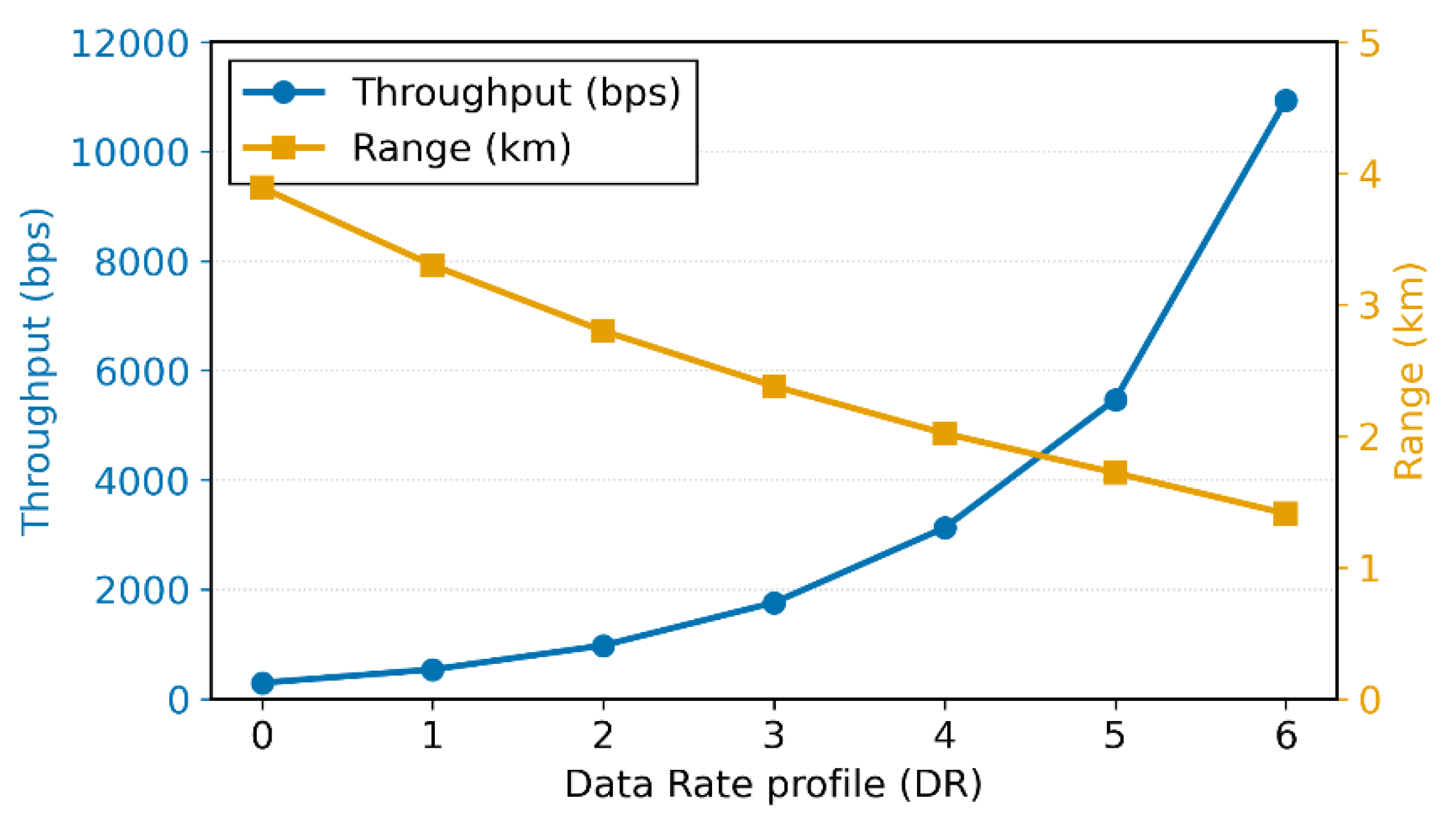
Figure 2.
Proposed multi-hop LoRa Stack.
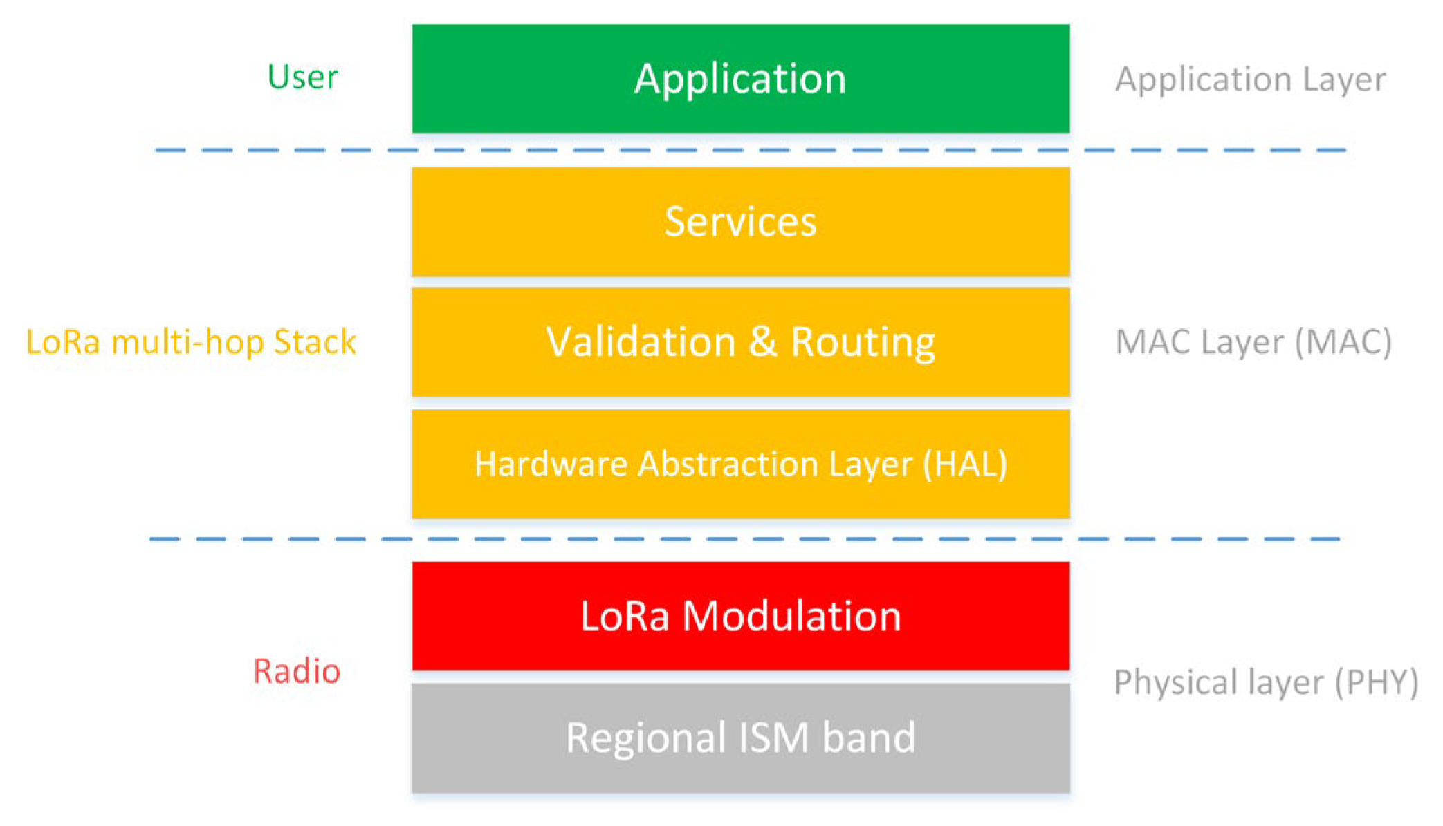
Figure 3.
Proposed multi-hop LoRa message.
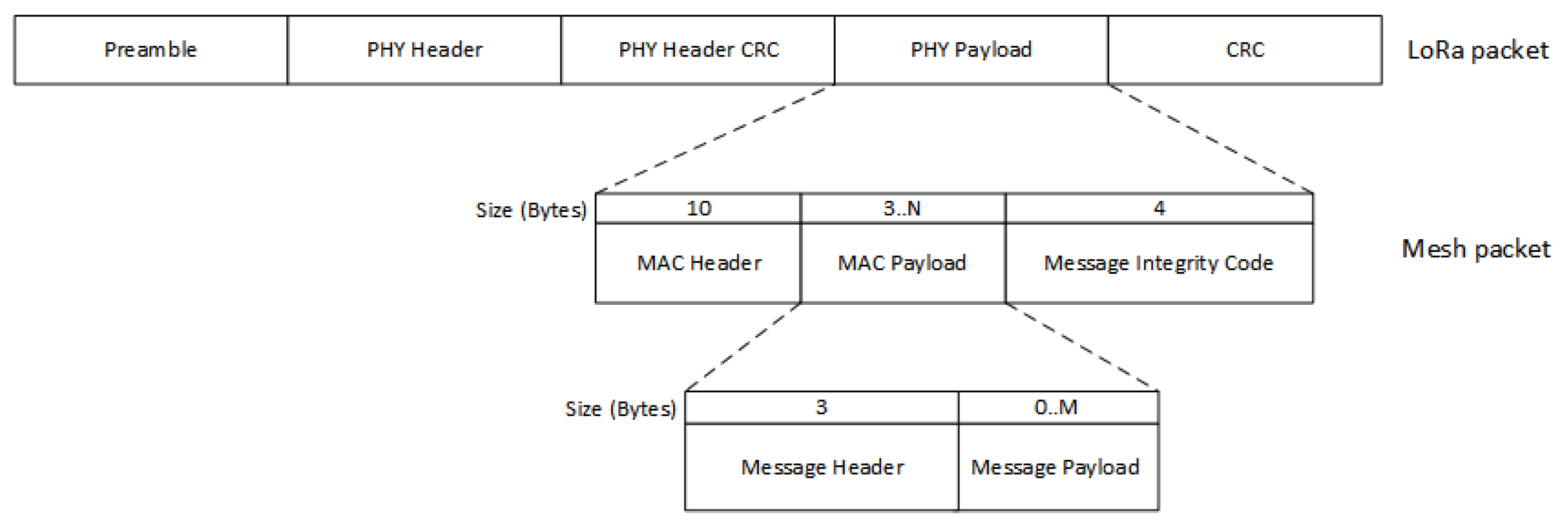
Figure 4.
Relay discovery messages exchanges diagram.
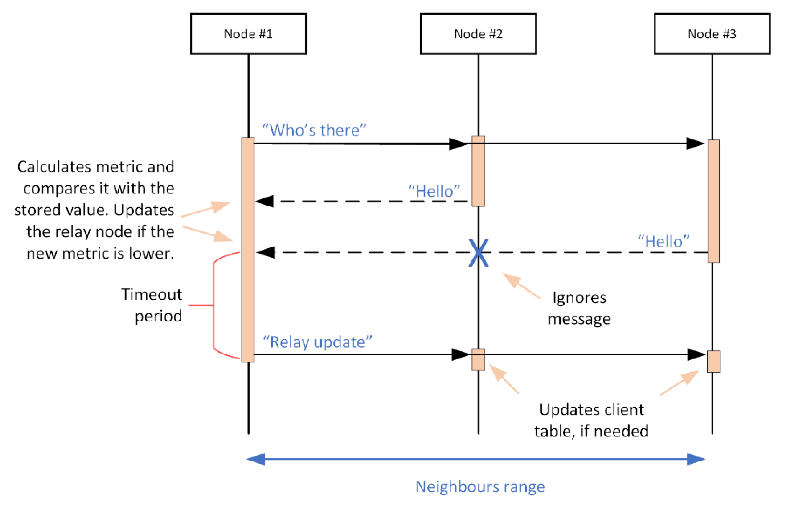
Figure 5.
Messages routing mechanism diagram.
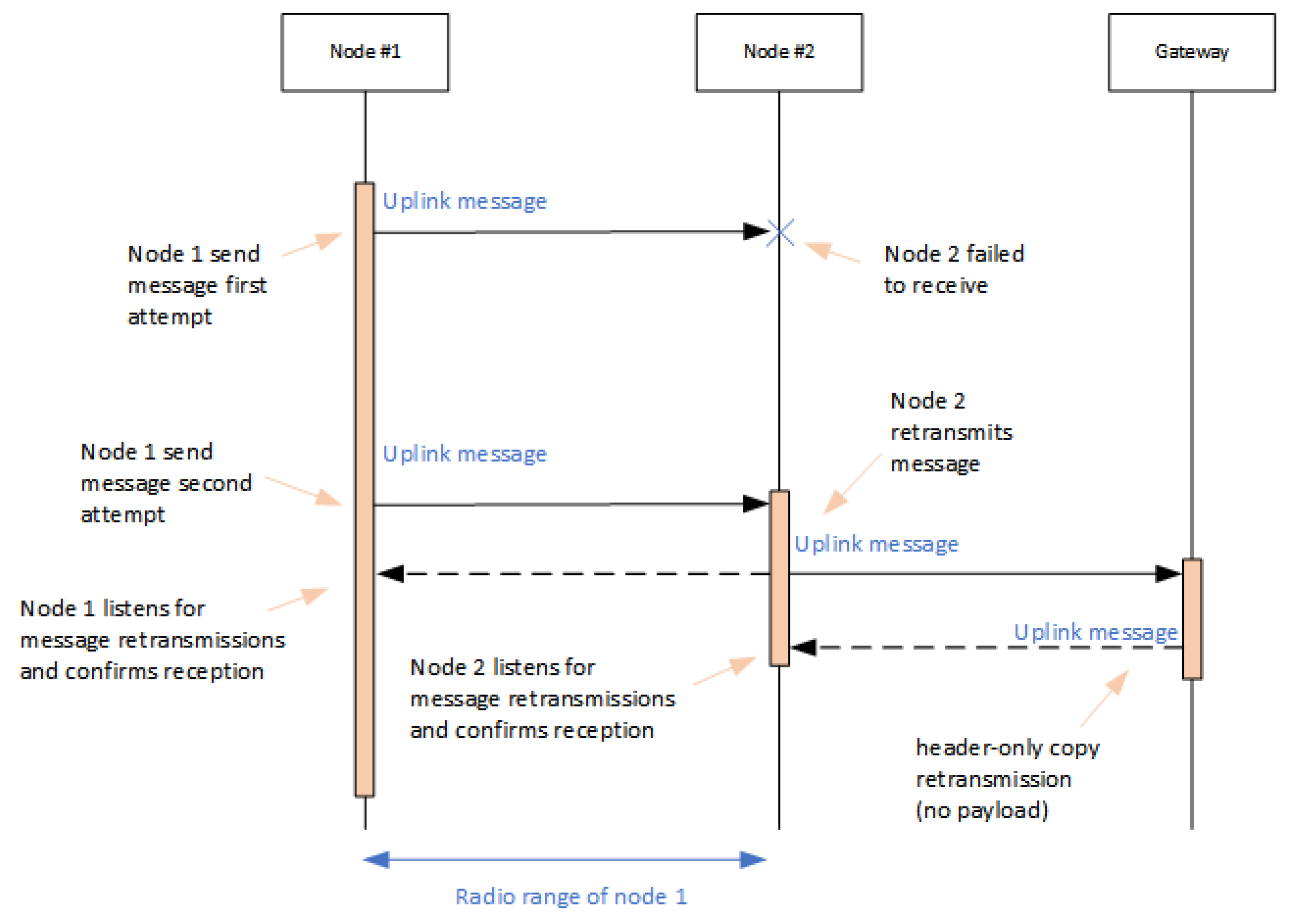
Figure 6.
Best Path Finding Algorithm GUI simulator snapshot. Node labels: h, hop count to the gateway; n, number of clients served (direct and indirect); c, path cost to the gateway.
Figure 6.
Best Path Finding Algorithm GUI simulator snapshot. Node labels: h, hop count to the gateway; n, number of clients served (direct and indirect); c, path cost to the gateway.
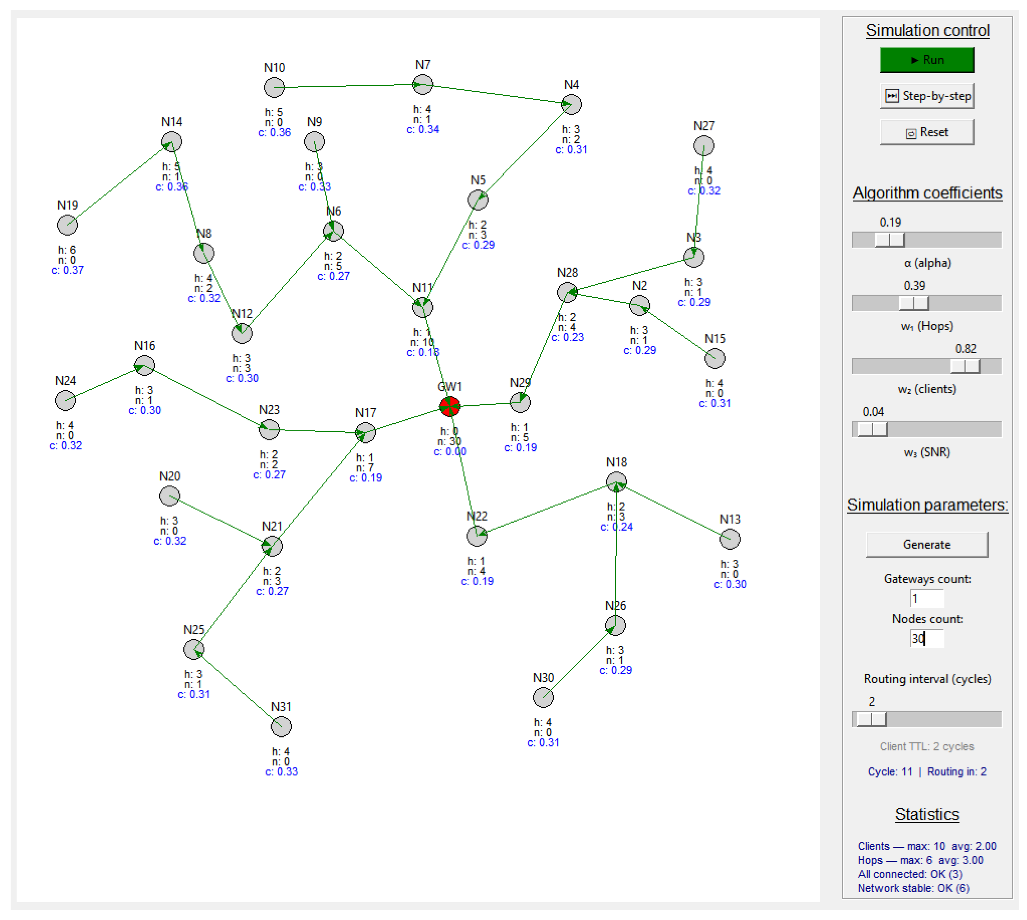
Figure 7.
Comparison of objective functions using max_clients and avg_clients as load term, versus the BFS baseline. (a) Average Hops over number of nodes. (b) Maximum Clients per Relay over number of nodes.
Figure 7.
Comparison of objective functions using max_clients and avg_clients as load term, versus the BFS baseline. (a) Average Hops over number of nodes. (b) Maximum Clients per Relay over number of nodes.
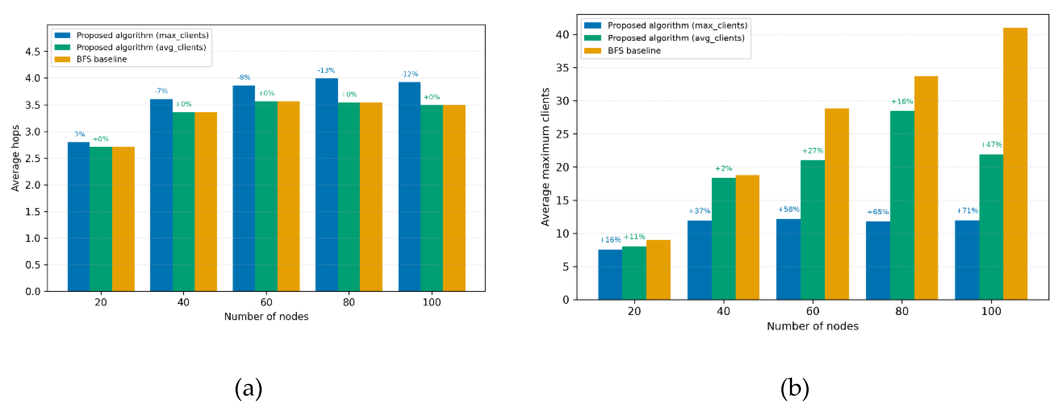
Figure 8.
Best algorithm parameters weights per number of nodes.
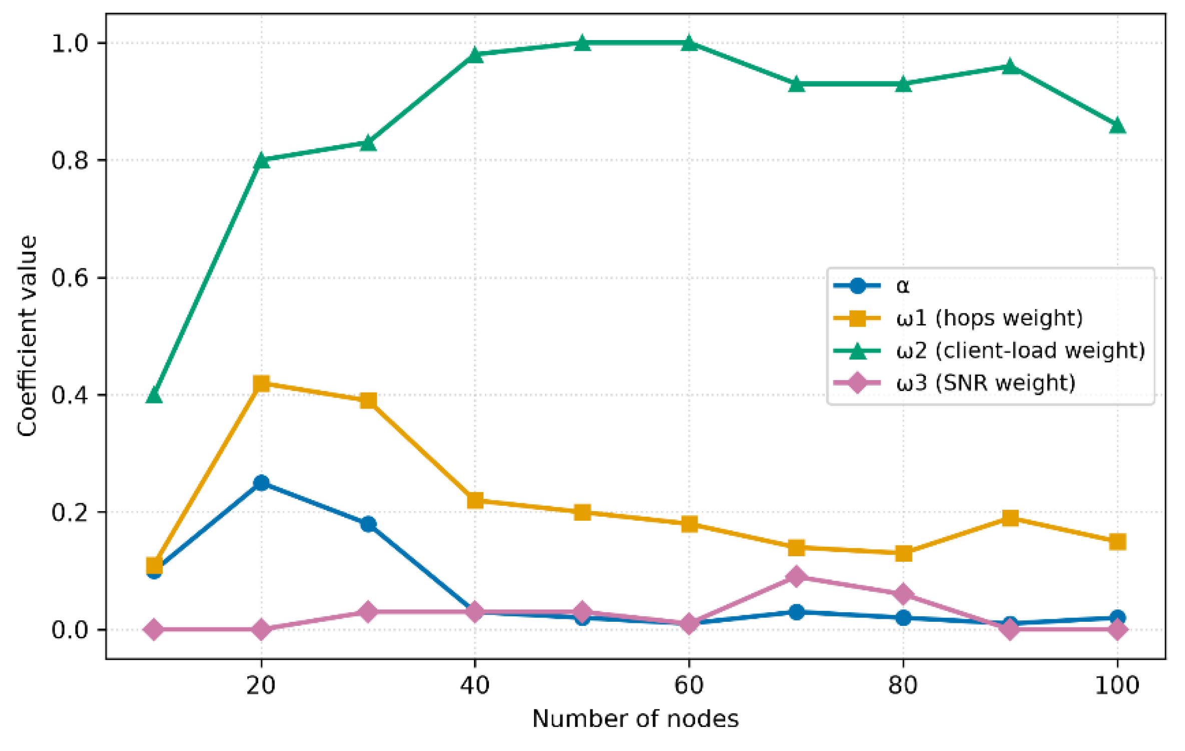
Figure 9.
Average hops evolution per number of nodes in proposed network versus BFS. Error bars: 95% confidence interval of the mean over the 30 topologies.
Figure 9.
Average hops evolution per number of nodes in proposed network versus BFS. Error bars: 95% confidence interval of the mean over the 30 topologies.
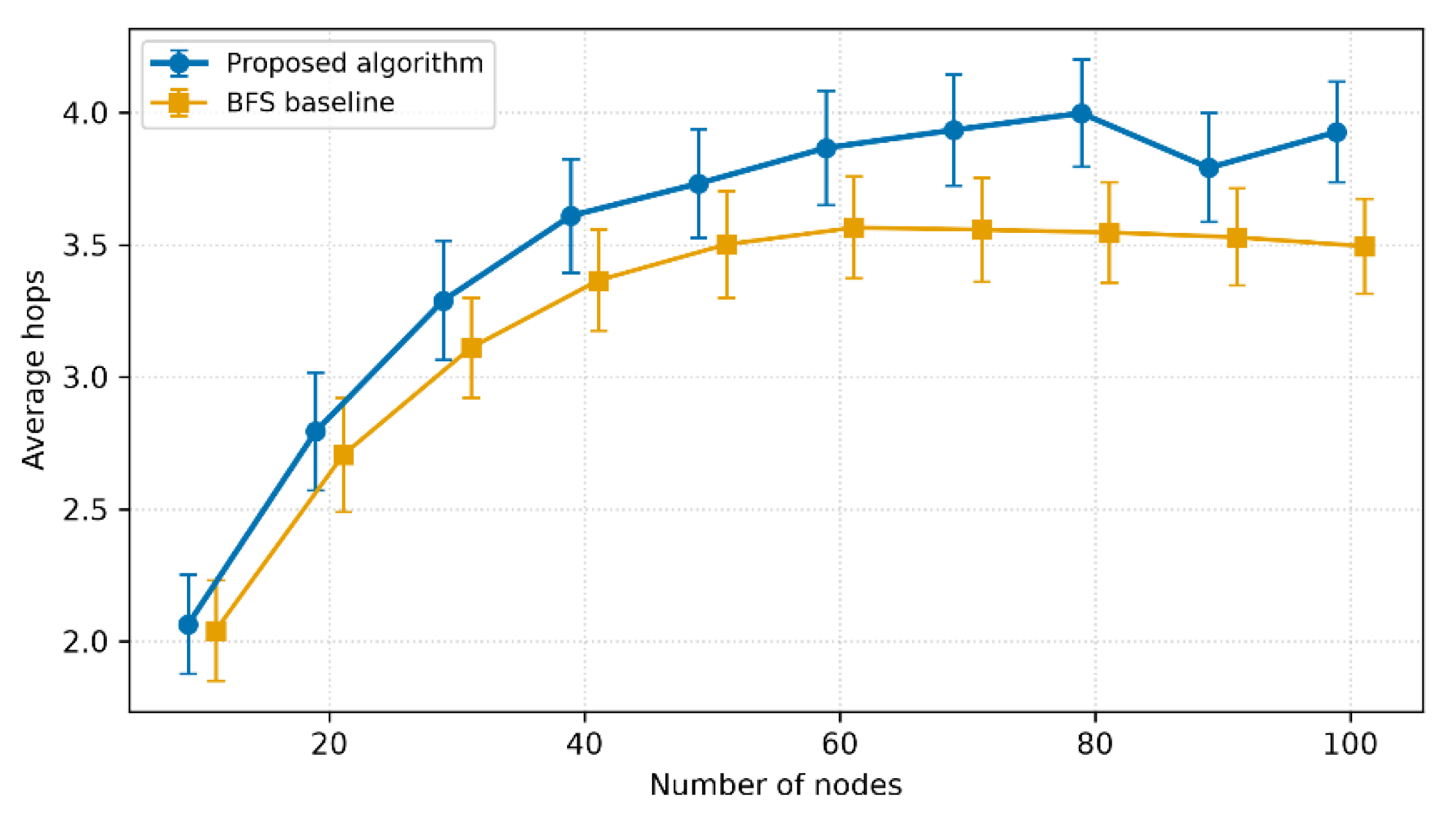
Figure 10.
Average maximum clients evolution per number of nodes in proposed network versus BFS. Error bars: 95% confidence interval of the mean over the 30 topologies.
Figure 10.
Average maximum clients evolution per number of nodes in proposed network versus BFS. Error bars: 95% confidence interval of the mean over the 30 topologies.
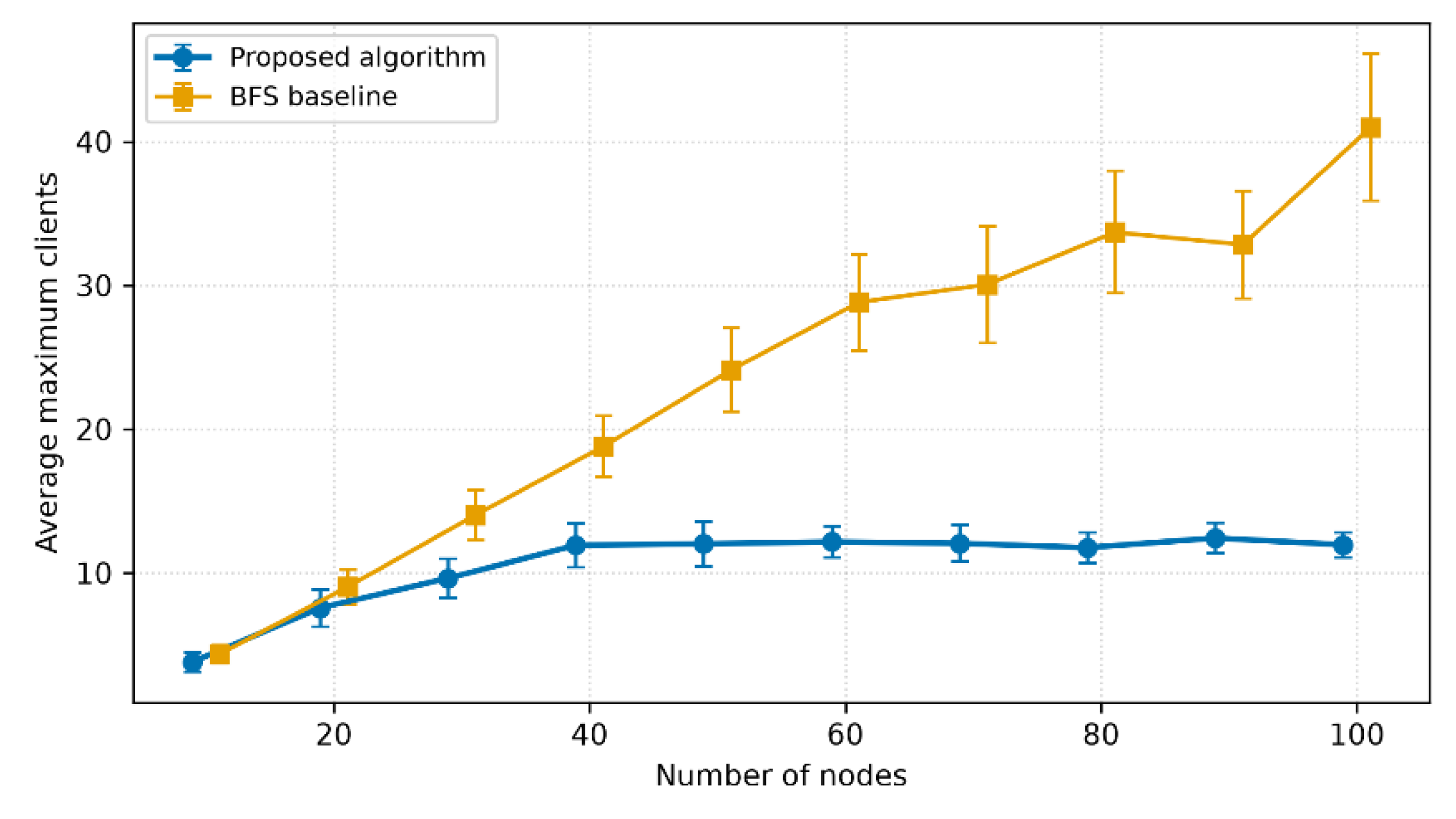
Figure 11.
Maximum clients distribution per number of nodes in proposed network versus BFS.
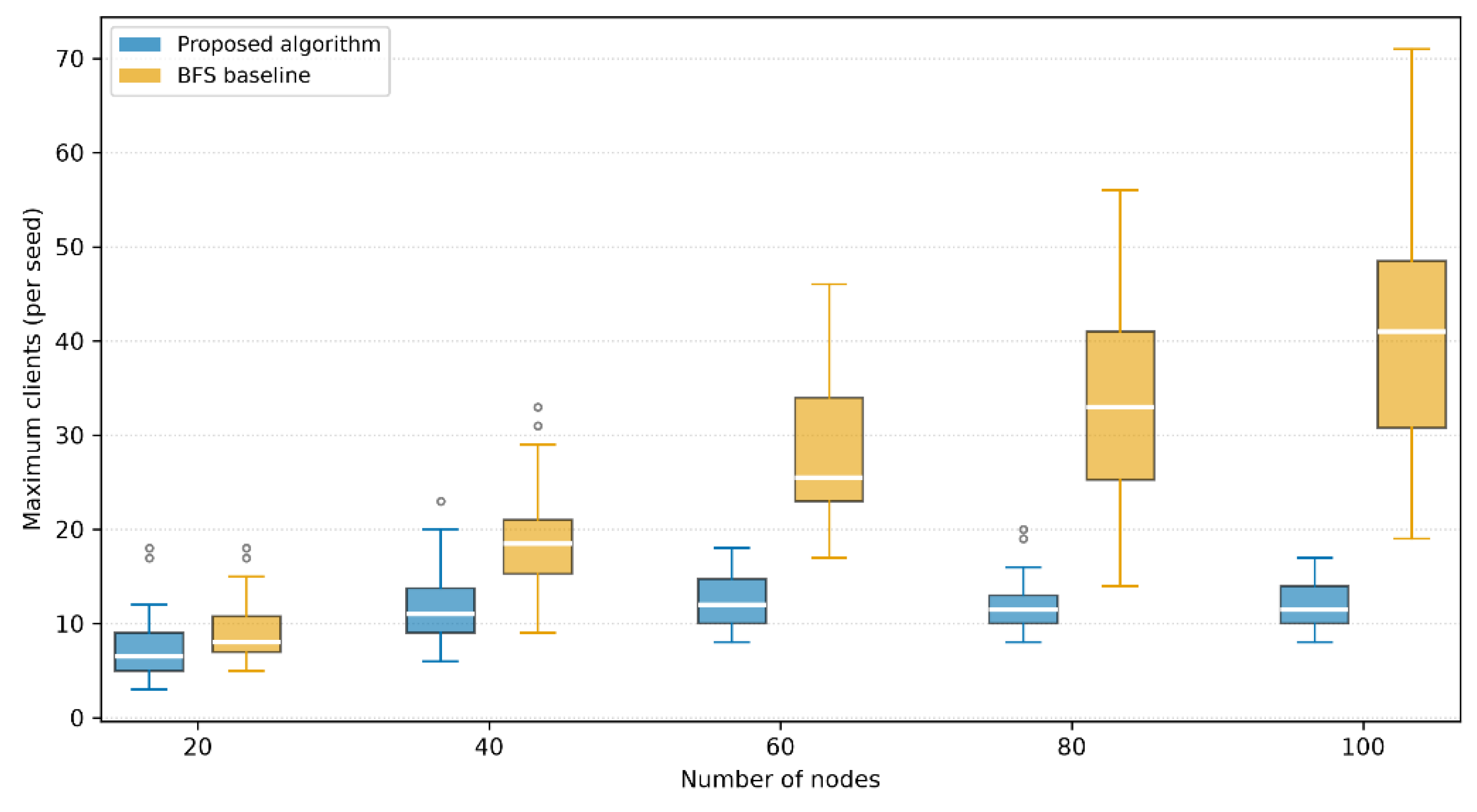
Figure 12.
Average cycles to full connectivity and to network stabilization per number of nodes.
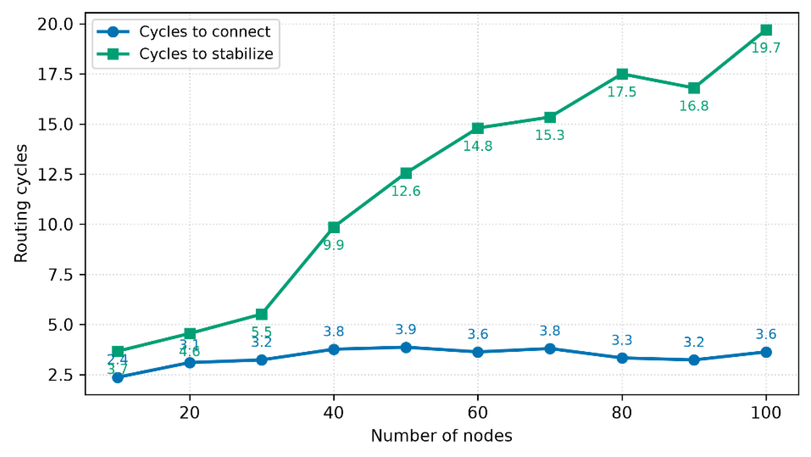
Figure 13.
Daily radio active time.
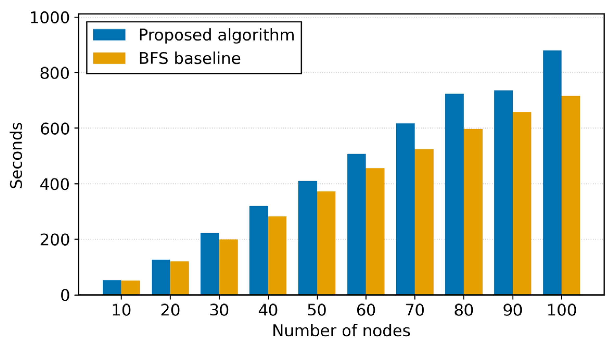
Figure 14.
Daily energy of the busiest node, split into transmission (TX) and reception (RX); the OFF-state energy (below 1%) is included in the RX segment.
Figure 14.
Daily energy of the busiest node, split into transmission (TX) and reception (RX); the OFF-state energy (below 1%) is included in the RX segment.
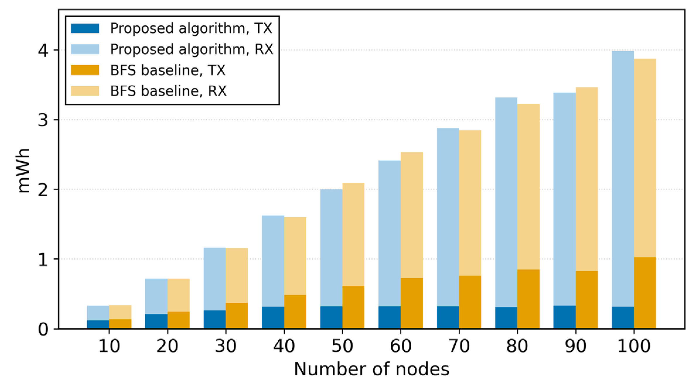

Table 1.
LoRaWAN EU863-870 Data Rates.
| Data Rate (DR) | Configuration (CR = 4/5) | Throughput [bps] | |
|---|---|---|---|
| SF | BW [kHz] | ||
| 0 | 12 | 125 | 250 |
| 1 | 11 | 125 | 440 |
| 2 | 10 | 125 | 980 |
| 3 | 9 | 125 | 1760 |
| 4 | 8 | 125 | 3125 |
| 5 | 7 | 125 | 5470 |
| 6 | 7 | 250 | 11000 |
Table 2.
SNR threshold for given SF [23].
Table 2.
SNR threshold for given SF [23].
| SF | 7 | 8 | 9 | 10 | 11 | 12 |
|---|---|---|---|---|---|---|
| [dB] | -7.5 | -10 | -12.5 | -15 | -17.5 | -20 |
Disclaimer/Publisher’s Note: The statements, opinions and data contained in all publications are solely those of the individual author(s) and contributor(s) and not of MDPI and/or the editor(s). MDPI and/or the editor(s) disclaim responsibility for any injury to people or property resulting from any ideas, methods, instructions or products referred to in the content. |
© 2026 by the authors. Licensee MDPI, Basel, Switzerland. This article is an open access article distributed under the terms and conditions of the Creative Commons Attribution (CC BY) license.
Copyright: This open access article is published under a Creative Commons CC BY 4.0 license, which permit the free download, distribution, and reuse, provided that the author and preprint are cited in any reuse.