

Submitted:
27 July 2026
Posted:
28 July 2026
You are already at the latest version
Abstract
Distributed acoustic sensing (DAS) deployed in submarine telecom cables is bound to revolutionize the earthquake monitoring routine currently performed by seismic network operators, particularly in domains where most of seismic activity is originated offshore. In this work we analyze one year DAS data recorded on a submarine telecommunication cable joining the Islands of Faial and Flores in the Azores, an area where seismic crisis of volcano-tectonic origin are frequent. We explore whether spatially decimated channels can be added to the operation routine without major changes. During the DAS operation the land network recorded 368 local and regional earthquakes. The best of these events were jointly analyzed and earthquake parameters were compared between original locations and adding DAS picks. Despite the larger picking uncertainty on DAS channels, adding P and S or S-wave picks only from DAS data showed a considerable improvement on earthquake parameters, reducing the error ellipse area and the focal depth uncertainty. These results demonstrate that in domains where offshore seismicity is a concern and submarine telecom cables are available, integrating DAS channels into the routine operation of seismic networks considerably improve the accuracy earthquake parameter estimation. A procedure to accomplish these results is presented.
Keywords:
distributed acoustic sensing (DAS)
; earthquake
; monitoring
1. Introduction
Distributed acoustic sensing (DAS) is a recent instrumental approach that enables the conversion of fibre-optic cables into dense arrays of acoustic sensors, e.g., [1]. This technology, based on the optical time-domain reflectometry (OTDR) technique, is attractive for marine environments where instrumentation is difficult to deploy.
DAS is particularly useful for monitoring offshore seismicity affecting oceanic Islands, where the seismic network is limited to land deployment. DAS extends the observation of ground motion (derived from strain or strain rate) on a spatial scale ranging from 10 m to 100 or 150 km or up to the first cable repeater from the landing site.
DAS offers an excellent opportunity to enhance the routine operation of seismic networks tasked with providing accurate earthquake parameters (epicenter, focal depth, magnitude) within a very short time after an event onset. Besides increasing the number of observation sites, the high density of observations enables the use of additional location tools, like beamforming, to refine the fast determination of earthquake source parameters. The big challenge is the huge volume of data generated by DAS and its real-time processing. One interim solution that has been adopted is to include a spatially decimated stream of channels into the seismic data collector of the monitoring agency. This approach has recently been implemented at IPMA—Instituto Português do Mar e da Atmosfera—(the Portuguese Agency for Earthquake and Tsunami Monitoring) with DAS data provided by the GeoLab cable [2].
We used the Azores Archipelago as the study area to explore the gains in seismic monitoring by extending observations offshore using DAS cable. In [3] we evaluated gains in simple geometric network performance parameters, such as the primary gap and the U-function defined by [4]. In [5] we went a step further, evaluating the gains in reducing location uncertainty, considering also the uncertainties in phase picking and propagation model through a Monte-Carlo simulation. In [3,5] the cable sensors were considered as identical to the ones installed on land and they were considered to be included in the routine operation of IPMA.
Using Rayleigh backscatter, DAS-measured phase changes originate from any change in the optical path of the laser light. These changes may have three different sources: temperature, strain, and pressure [6,7].
When the fiber is strained, the optical path is perturbed by several effects, whose combination is a function of the strain-optic tensor, and results in a strain sensitivity, e.g., [8], that depends on Pockel’s coefficient, the refractive index of the fiber, the gauge length, and the wavelength of the laser light.
[9] also showed that the strain resulting from longitudinal (P) and transversal (S) plane waves incident on a cable has a marked angle dependence with well-defined null directions where no signal should be recorded. Furthermore, obtaining ground velocity from strain or strain-rate measurements requires knowledge of the apparent phase speed along the cable for each seismic phase recorded.
Single-channel DAS data is not identical to a one-component horizontal seismometer recording and a real data analysis is required to evaluate its added value to earthquake monitoring. This work leverages data acquired within the MODAS project (Monitoring the Ocean with Distributed Acoustic Sensing) to conduct this analysis under realistic conditions.
This article begins by describing the Azores regional setting and the experimental framework for earthquake monitoring. We then summarize the main properties of the DAS data recorded and define a strategy for the selection of the decimated channels. Likewise, we examine all DAS recordings of seismicity recorded by the land network and obtain an estimate of the sensitivity threshold as a function of magnitude and distance. Next, we relocate the high S/N events using the decimated channels and two sets of cable phase picks (P + S or S only), thereby evaluating the added value of DAS data. Finally we discuss, in the light of the obtained results, how DAS observations from offshore cables can provide valuable information for both real-time monitoring and deferred-time investigations of offshore seismicity, particularly in ocean islands settings such as the Azores-Faial where seismic monitoring is largely restricted to land-bases stations.
2. Setting of the Investigated Area
Materials The Azores archipelago straddles across three tectonic plates, North America, Eurasia and Nubia (Figure 1) encompassing a triple junction with two well-defined spreading ridges and a third branch, the Terceira rift, that can be considered as an ultraslow oblique spreading centre [10,11]. The islands of Flores and Corvo lie on the American plate, while the remaining islands lie on the elevated bathymetric Azores Plateau, the result of the triple junction evolution since it jumped to its current location. The Terceira Rift is characterized by seismic and volcanic activity.
Seismicity in the Azores Plateau is dominated by low to moderate magnitude events, with occasionally large (M~7) magnitude events causing destruction and casualties [11]. The most recent strongest earthquakes include the 1st January 1980 Terceira event [12] and the 9th July 1998 earthquake [13]. The seismicity in the Azores Plateau is confined along a wide, elongated band following the islands’ alignment (Figure 1).
The Azores archipelago has a volcanic origin, and volcanic eruptions are common in historical times. The most recent on-land eruption was the Capelinhos surtseyan–strombolian eruption and phreatic explosions in 1957/1958 (eastern Faial Island) [14]. The volcanic and tectonic setting along the Terceira Rift is the explanation for the occurrence of frequent seismic crises, in addition to those associated with large tectonic earthquakes, which are of type (1) or type (2), according to the Mogi classification scheme [15]. Type (3) seismic sequences don’t have clearly stronger events and can last for months or years. The Serreta seismic crises located West of Terceira Island, could be associated with an offshore volcanic eruption [16], but most sequences do not result in extrusive activity. NW of Faial Island, we find an area where a seismic sequence lasts for several years with the occasional occurrence of felt earthquakes on the island (Figure 1). As these seismic swarms occur mostly offshore, their detailed seismological study remains challenging because seismic stations are located only on land.
IPMA is the Portuguese National Agency for Earthquake monitoring, and it currently operates 15 short-period seismometers, 11 broad-band seismometers and 28 strong-motion accelerometers in the Azores [17] (Figure 1). Despite the large number of operating instruments, the network geometry is clearly unfit to provide well-resolved epicenter and focal depth estimates of earthquakes that lie outside the islands’ alignment. We may use the event gap parameter (the maximum angle between consecutive recording stations) or the U-function defined by [4], which compares the event to station azimuth distribution with the ideal uniform distribution.
Taking as reference the ISC catalogue (http://www.ISC.ac.uk) from 1960 to 2026-03-30, we identified, within the study area, 8658 earthquakes with M > 3 and 80 with M > 5 (Figure 1). Defining the best constrained area as the one with gap < 180º, we infer that 71% of the M > 3 seismicity and 80% of the M < 5 seismicity are outside this area (Figure S1a).
For the [4] U-function, the well-constrained area is the one with U < 0.35. This criterion is more demanding than the gap and only 0.5% of the M > 3 seismicity is inside the best-constrained area, while 1.4% is inside for the M > 5 seismicity (Figure S1b).
In this work, we move beyond geometric considerations and investigate the contribution of DAS to monitoring offshore seismicity using real data acquired within the MODAS project.
3. The Experimental Setup
Within the framework of the MODAS project we instrumented the subsea telecommunication cable between Faial and Flores (Figure 1), which is operated by Fibroglobal (Fibroglobal Comunicações Eletrónicas S.A. a FastFiber Company, Rua João de Lemos, nº 3, 1300-324 Lisboa, Portugal). We installed one DAS interrogator for a period of one year at the Faial Cable Landing Station to investigate the contribution of DAS technology to the knowledge of seismicity, physical oceanography and marine mammal passive acoustic monitoring.
The submarine cable used in this study is 170 km long and contains no repeaters. It was laid on the ocean floor, with depth increasing rapidly away from the coastline (Figure 2). DAS data were collected on a single-mode dark fiber from an unused telecom fiber pair. The DAS interrogator connected at the Faial cable landing station was a HiFi Distributed Acoustic Sensor (HDAS. which is a chirped-pulse ϕ-OTDR interrogator prototype developed by UAH and CSIC [18]. In this experiment, the HDAS interrogated ~50 km of cable with a 10 m gauge length and 10 m spatial sampling, yielding 4992 channels, at a sampling frequency of 1 kHz (Figure 2). The strain time series were later down sampled to 50 Hz due to limitations in local data storage, a frequency that does not compromise the major objectives of the MODAS project. The HDAS operated from December 2023 to December 2024, but a continuous recording was not possible due to local constrains (Figure S2). Over the deployment period, a total of 6.68 TB of DAS data was obtained, typically 40.7 GB/day.
For calibration and validation of the HDAS recordings, the MODAS project deployed two OBS units developed at IDL and designed for long-term offshore monitoring. Each OBS records ground motion with a broadband seismometer and seismic–acoustic signals in the water column with a hydrophone (Figure 2). The OBS location is a few hundreds of meters from the cable. The 3-C seismometers and the hydrophones sampled at 250 Hz and 100 Hz, respectively. The OBS recorded data continuously for 5 months from July 2025 to November 2025. A summary of the HDAS and OBS data acquired within the MODAS project is shown in Figure S2. With regard to the HDAS, we obtained 148 full days and 35 partial days of data. Further details of the MODAS experimental setting can be found in [19].
HDAS data required some pre-processing before being available in standard formats, like miniseed, seg-y or HDF-5. The data is recorded on a compressed proprietary format, with all channels stored in one-minute-long files. The proprietary application uncompresses the data and generates one file per channel in binary format. The length of each file is user-defined and independent of the original file lengths. Finally, these binary files were converted into a standard format for quality control, further processing, and analysis. This procedure is computationally expensive on a PC, and only a few 24-h files were generated. Our analysis was based on short time event data pre-processing.
During the period of HDAS operation, the land stations on the neighboring Islands, Faial and Pico, recorded 368 earthquakes, local, regional and teleseismic (Figure S3). Of these, 229 events were also recorded by the MODAS OBS. In this study the full set of 368 events is analyzed.
4. HDAS Quality Control
We first selected a time interval without any earthquakes and computed the RMS of each channel to obtain an initial idea of the noise level in the HDAS data. The resulting RMS is shown in Figure 3a while the corresponding waveforms are shown in Figure S4. Figure 3b displays the cable depth profile.
We identified four domains: (1) the land section with recognizable anthropogenic noise (car traffic); (2) the shallow water section, water depth smaller than 200 m, where the HDAS signal is dominated by swell; (3) the near-deep water section where RMS noise level is the lowest, and where ground motion is expected to be better recorded; (4) the far deep water section where RMS noise level increases, likely due to the HDAS interrogator self-noise. Here, the noise level after an offset of 26 km seems to increase exponentially with offset.
Within domain (3), we identify two sections of the cable with high RMS noise, labeled as (X). These are also clearly identified on the waveforms (Figure S4). Both sections also coincide with a change in the seabed relief, and they are interpreted as sections where cable-to-seafloor coupling is poor or even cable suspensions, with the RMS noise level caused by bottom currents acting on the cable. This plot also allows the identification of the first channel in the water (at 198 km from the landing station), marking the sharp transition between sections (1) and (2) in the cable.
The waveforms presented in Figure S4 also display horizontal bands of low-frequency noise common to all channels. These are interpreted as common mode noise. We then checked the low-frequency PSD of channels located in zone (3) of the cable to assess whether this noise could impair the recording of low-frequency signals, either from earthquakes or from an oceanic origin. The result is shown in Figure 4. It displays a noise increase with 1/f for frequencies smaller than 1 Hz which precludes the use of this dataset for the analysis of low frequency signals, like those generated by teleseismic earthquakes.
One of the main advantages of DAS recordings in general is the possibility to use the high spatial density of data, channels spaced every 10 m in our case, to apply multi-channel signal improvement algorithms or enhanced source location routines, like beamforming. These rely on the similarity between neighboring channels. To assess this feature in our data, we selected the HDAS recordings of one clearly recorded earthquake and plotted two sections of 300 channels (spanning 3 km), located close to the deployed MODAS OBS. These recordings are shown in Figure 5.
We observe a very high variability in channel-to-channel amplitude. This high variability can also be noticed in more detail when we compare the HDAS channel data with OBS waveforms, as shown in Figure S5. The Azores Islands and the Azores plateau, where the Faial-Flores cable was deployed have a volcanic origin. For this reason, a rough sea bottom relief is expected. This may be the main reason for the channel-to-channel signal variability at 10 m spacing, with a considerable change in cable coupling. This motivated the development of a strategy for selecting the best HDAS decimated channels for earthquake analysis. For the same reason, we didn’t apply multi-channel enhancement routines that are based on signal similarity for that analysis.
5. Earthquake Detectability by HDAS
In this section, we evaluate how HDAS recordings compare with the land based seismic network waveforms. During the HDAS operation, the IPMA network in Faial and Pico recorded 368 local and regional earthquakes. Here we disregard the teleseismic events due to the lack of a low-frequency response from DAS. The smallest magnitude present in the IPMA catalogue is −0.6.
To evaluate HDAS recordings, we select two 300-channel HDAS sections (corresponding to 3 km of cable) near the MODAS OBS locations. These were identified as sections CAB01 and CAB02. For each event identified by IPMA, we extracted 10-min windows of HDAS data, starting 3 min before the event’s origin time. Each of these data sections was then examined to identify P and S phase arrivals after applying a 2-Hz high-pass filter. Based on the visual quality of the data, we classified the HDAS recordings into 5 categories:
(1) Very Good. Meaning that both P and S waves can be seen on both sections.
(2) Good. If only one section allowed the identification of P waves, while both sections allowed for clear S waves.
(3) Fair. If only S waves are seen on both sections.
(4) Poor. If only weak S waves are identified.
(5) No. If no seismic signal could be identified.
We note that this classification scheme accounts for the easier detectability of S waves by the HDAS than P waves, due to its polarization in the horizontal plane since HDAS acts as a horizontal linear sensor. Waveform examples for categories (1), (2) and (3) are presented in Figure S6. The distribution of the 368 events in the quality categories is as follows:
| Very Good | 51 (14%) |
| Good | 44 (12%) |
| Fair | 130 (35%) |
| Poor | 66 (18%) |
| No | 77 (21%) |
We observe that for 225 events (61%), clear S waves can be identified in both cable sections, whereas P waves can be clearly identified in both sections for 51 events (14%).
To assess the detectability of the HDAS, we used as reference, the closest distance of the epicenter to the cable and plotted the magnitude versus distance for all categories in Figure 6.
We note that the average trend of magnitude vs. distance is nearly identical for all classified events. As expected, when event magnitude increases, the recoded quality also increases, about 1.5 magnitude degrees from “No” to “Very Good” recordings. Nevertheless, there is a large dispersion of values to consider, with some “Good” events recorded below the “No” average. Taking the “Good” as a reference for the usefulness threshold, then we may infer that this threshold is, on average, 1 magnitude degree above the land network detection capability. The latter is outlined by the lower envelope of the magnitude distance plot for all qualities (continuous black line in Figure 6).
6. Choice of HDAS Channels for Earthquake Analysis
We consider that the simplest integration of HDAS data into routine earthquake analysis workflow, as it is done by IPMA, is to add a set of spatially decimated channels to the data collector. In this work, we investigate the added value that could be provided by HDAS channels 1 km apart, resulting in a total of 49 new channels to be included in the earthquake analysis.
Considering the waveform variability of the HDAS data (see Figure S7), we proceeded to choose the decimated channels based on some data propriety instead of choosing a regular channel spacing blindly. Our first choice was to use the channels with the smaller RMS noise level within an acceptable bin around each kilometer mark. However, this selection doesn’t properly account for differences in cable coupling between closely spaced channels, as illustrated in Figure S8. We finally decided to pick the channels one by one as those with the maximum S/N computed from a well-recorded earthquake. The procedure is illustrated in Figure 7. A comparison of the choices based on RMS or S/N is presented in Figure S9.
7. Determination of Earthquake Event Parameters
To investigate the contribution of the HDAS decimated channels selected in the previous section to the determination of earthquake source parameters, we selected 31 offshore events classified as “Very Good”, the most likely to see significant improvement, out of a total of a selection of 244 offshore earthquakesThe selection is shown in Figure S10. We recall that the “Very Good” events correspond to those for which clear P and S wave arrivals could be identified in the channels around the two OBS locations (see Section 3).
Our starting earthquake location is the one provided by IPMA, with the phase arrivals picked by the seismic network operators. These earthquake parameters are identified as LOC00. They constitute the background against which any improvement is assessed (Figure S10).
Next, we include the HDAS waveforms into the data collection and pick P and S waves on as many channels as possible. Given the characteristics of HDAS recordings, the picking precision is lower than for the land stations, but this is expected to be compensated by adding many 10s of new picks. Then we relocate the events, merging all picks, IPMA + HDAS-P + HDAS-S and obtain a catalogue named LOC01.
Given that S-waves are generally more likely to be well recorded than P-waves on DAS instrumented submarine cables, we relocate the same selection, adding only the HDAS-S picks, therefore obtaining a new catalogue LOC02. Other combinations of picked phases were also tested, such as using only the P and S HDAS phase picks. However, these tests did not provide any improvement, with most obtained locations showing large uncertainties.
We present this procedure as Supplementary Figures, beginning with a selection of HDAS P and S picks in Figure S11. As expected, S-waves are better identified than P-waves, which are not seen on all channels. Some picks have an uncertainty value as estimated by the operator. Figure S12a–c, show the epicenter ellipse error estimated by the location code [20] for catalogues LOC00, LOC01 and LOC02. In this example, we observe that using HDAS P- and S-wave picks reduces considerably the area of the uncertainty ellipse and moves the epicenter nearly outside the original ellipse. Using only HDAS S-wave picks, moves the epicenter outside the original uncertainty ellipse, also reducing its area by a smaller amount.
8. Summary of Earthquake Analysis
In this section, we summarize the results obtained from the relocation of the 31 “Very Good” events selected above. The number of phases picked by the land-based network and by the 49 HDAS channels is presented in Figure 8.
On land, the phase picking is dominated by a set of ~10 stations. Only 5 stations’ picks were used for most of the events. S waves are slightly more picked than P waves.
On the HDAS channels, S wave picks dominate, and all channels provided useful S picks for more than 50% of the events. Surprisingly, P and S wave picks could be obtained from the noisiest domains of the cable, domain (2) dominated by swell noise, and domain (4) with increasing instrumental noise. In domain (3), the one with the low noise, many channels provided a large number of P-wave picks. This number falls rapidly in domains (2) and (4). The noise on the cable seems to influence more the P-wave picking than S-wave picking.
We quantify the epicenter uncertainty for the 3 sets of picks, LOC00, LOC01 and LOC02, by computing the error ellipse and its area. One example of the 3 locations obtained is shown in Figure S12. The epicenter location and error ellipses for the 3 sets are shown in Figure S13. We can visually see that most locations had reduced uncertainty with HDAS picked channels, even when only S-waves are used on HDAS. This improvement can be more accurately assessed by comparing the areas of the error ellipses across the 3 sets of picks. This comparison is illustrated in Figure 9.
We note that most events show a considerable reduction in the uncertainty area between the original locations and those obtained with HDAS P and S picks. Only a few of them show an increase in the uncertainty area using HDAS (Figure 9a). The same conclusions apply when we use HDAS S-wave picks only (Figure 9b) with a smaller emphasis.
The new sets of picks also imply a displacement of the epicenters. This effect is shown in Figure S14, which compares the IPMA original locations with the new locations from HDAS P and S picks. In general, epicenter shifts are relatively small (less than 10 km), but a few events have a larger displacement.
To evaluate the contribution of HDAS to reduce the epicenter uncertainty, we compute the percentage variation in error ellipse area between the IPMA catalogue and the set of locations obtained from IPMA and HDAS P & S picks. The results are presented in Figure 10. Only 4 events show an increase in error area when using HDAS picks.
Besides the improvement in epicenter quality, DAS is also expected to reduce the focal depth uncertainty of offshore events, as evaluated by [21]. The comparison with the investigated dataset is shown in Figure 11. We note that, due to the poor azimuth coverage for many of the selected events, this uncertainty could not be estimated without inclusion of HDAS data. For the 11 events where such a comparison was possible, we note that 7 events showed a remarkable error decrease, whereas 4 events showed only minor or no error decrease.
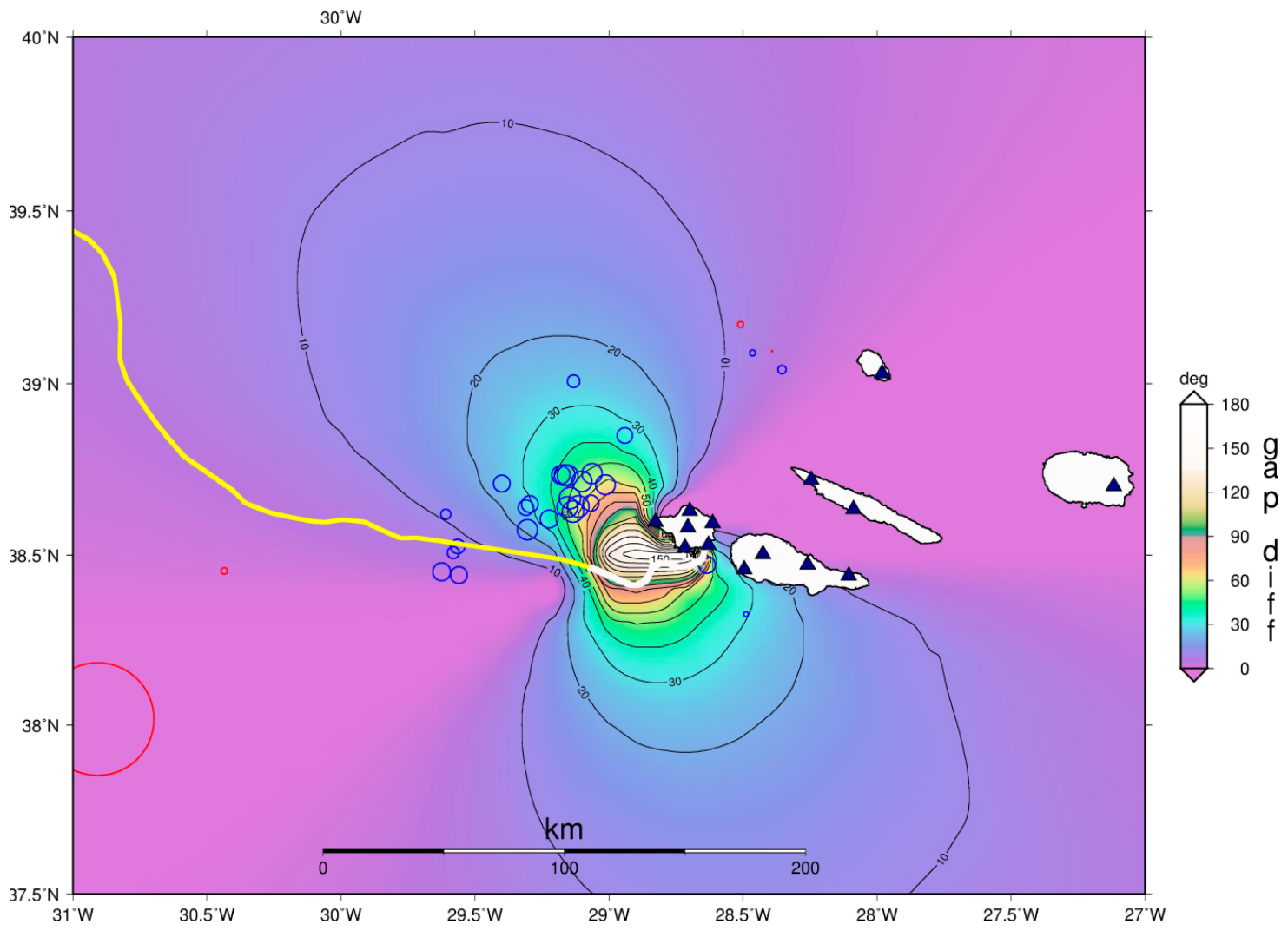
Finally, we seek some explanation for the poor performance of adding HDAS to the analysis set that we identified for some events. By comparing the LOC00 and LOC01 network gaps, we verify that the events with poor performance are in areas where the HDAS provided very little gap reduction (smaller than 10º), as shown in Figure 12. We may infer that, under these conditions, the larger uncertainty in picking HDAS phases counters the small improvement to be expected from the gap reduction.
9. Discussion and Conclusions
Distributed Acoustic Sensing is a technology that is revolutionizing the observation of the Earth. When deployed on submarine telecommunication cables, DAS provides very high spatial strain or strain rate recording, with sensing ranges up to a maximum distance of 170 km along the cable, or up to 300 km with Raman amplification. For earthquake monitoring applications, DAS allows for highly sensitive event detection, e.g., [21] and enables the use of multichannel processing location algorithms, like beamforming, e.g., [22].
DAS will likely make an enormous impact on the real-time earthquake analysis that is currently performed in the seismic network operations centers. This promise will probably take a while, as network operators adapt to the new technology and address the major challenge of the huge volumes of data acquired by DAS, needing to be processed in real-time.
Meanwhile, a simpler approach can be followed, without major changes to the standard operating procedures of the responsible agencies. Some DAS interrogators can make available to the seismic data collectors a spatially decimated dataset in real-time using standard seismic format [23]. The new station spacing is to be chosen by the stakeholder, for example 1 km (as here) or 5 km [23]. This new information, though limited in distance to the coast, can make a significant contribution to the quality of earthquake analysis, as its relevance increases in regions that are affected mostly by offshore seismicity, like in volcanic Islands, for example in the Azores and Canaries Archipelagos in North Atlantic.
In this work, we investigated, in the Azores region, the contribution of DAS decimated channels to the determination of earthquake parameters by the IPMA agency, responsible for seismic monitoring. For this purpose, we used DAS data recorded during one year along the telecom cable between Faial and Flores, covering a total monitored length of 49 km. The interrogator was a HiFi Distributed Acoustic Sensor (HDAS) prototype developed by UAH and CSIC.
Using HDAS recordings, we could clearly identify 3 oceanic domains: (2) shallow water with amplitude dominated by swell, (3) deep ocean with low noise at middle offsets and (4) deep ocean with instrumental noise increasing with offset. We could also identify small sections of the cable with very high noise levels, likely representing suspended sections vibrating in response to deep-ocean currents.
As regards HDAS waveforms, we found very low correlation between neighboring channels 10 m apart, which may hinder applying advanced multichannel processing algorithms for signal enhancement.
We also found low-frequency common mode noise in HDAS data. Adding to the 1/f noise increase for frequencies lower than 1 Hz, we may conclude that this interrogator is not adequate to record low-frequency signals like tele-seismic earthquakes, infragravity waves and tsunamis.
The HDAS channel amplitude is highly variable on a ~200 m scale, which we interpret as a result of variable cable coupling on a volcanically derived, rough seafloor.
Using events detected by the IPMA land seismic network as a reference, we found that 61% of these earthquakes could be recorded by HDAS with useful S-waves. Only 26% of the events were recorded by HDAS with useful P and S waves.
The sensitivity of HDAS, considering that it is useful when good S-wave picks are obtained (at least), is quite variable, but we estimate it to be 1 degree higher than the land network, for the same distance range. Sensitivity of HDAS is typically M~1 for D < 40 km; M~2 for D = 100 km; and M~3 for D = 200 km.
When picking seismic waves on HDAS, the only processing step for the analysis of local and regional earthquakes was a 2 Hz high-pass filter. This step also attenuated the common mode low-frequency noise.
To facilitate the integration of HDAS data into routine earthquake monitoring, we considered adding a spatially decimated set of channels with an approximate spacing of 1 km. The decimated channels were selected individually based on the highest signal-to-noise ratio (SNR) within a search window centered on each kilometer mark.
We could perform P and S wave picks on HDAS even on channels belonging to higher noise levels, like (2) and (4).
We consider that individual picks on HDAS have greater uncertainty than those obtained from conventional land stations. However, this limitation appears to be compensated by the large number of closely spaced sensing channels.
By investigating in detail a set of 31 events where good P and S-waves could be picked on HDAS, we verified that epicenter uncertainty, as measured by the error ellipse area, is considerably reduced by HDAS. This improvement is also verified when only S-wave picks from HDAS are used, which we expect to be the most frequent case. The uncertainty ellipse area is, on average, reduced to ~26% its original size. These considerations should apply to 61% of the local and regional events detected by the land network offshore, where mostly HDAS S-wave picks are available, despite the larger uncertainty in HDAS individual phase picks.
Finally, the reduction in network azimuth gap achieved by combining the land seismic network with the HDAS channels appears to be the dominant factor contributing to the improvement in earthquake location. Cases in which the inclusion of HDAS data increased the location uncertainty were restricted to offshore regions where the reduction in network gap was negligible or absent.
The telecommunication cables that serve the Azores Archipelago will be replaced soon, in the next couple years. This offers the opportunity to add dark fibers that can be monitored by DAS on the landing sites. In this work we demonstrate the added value of such addition for the monitoring of offshore seismicity. Furthermore we present a procedure to accomplish these results that can be replicated in other oceanic domains without major changes to the standard operation routines of seismic network centers.
Supplementary Materials
The following supporting information can be downloaded at the website of this paper posted on Preprints.org.
Author Contributions
L.M. writing—original draft preparation; C.C. conducted the OBS experiment and performed OBS data processing and analysis; A.L. DAS analysis software development; S.G. DAS data processing and QC; S.S., H.F.M., O.F., DAS data acquisition, processing and analysis; F.C. Seismic data analysis from land network; M.N. DAS data analysis. All authors contributed to the preparation of the MODAS proposal that was the main supporter of the work. All authors have read, commented, proposed corrections and agreed to the published version of the manuscript.
Funding
This work was funded by FCT, I.P./MCTES (PT) through national funds (PIDDAC): LA/P/0068/2020 (https://doi.org/10.54499/LA/P/0068/2020), UID/50019/2025—(https://doi.org/10.54499/UID/50019/2025), and by the European Union—NextGenerationEU under projects UID//PRR/50019/2025 (https://doi.org/10.54499/UID/PRR/50019/2025) and UID/PRR2/50019/2025 (https://doi.org/10.54499/UID/PRR2/50019/2025, by the MODAS project 2022.02359.PTDC, and by EC project SUBMERSE project HORIZON-INFRA-2022-TECH-01-101095055. AL acknowledges funding by the ECHO project 2024.13655.PEX (DOI: 10.54499/2024.13655.PEX). HFM acknowledges financial support from the MCIN/AEI/10.13039/5011000 11033 and European Union «NextGenerationEU»/PRTR under grants RYC2021-035009-I, CPP2022-009772, PID2024-162301OA-C22, CPP2024-011822. This work is co-funded by Component 5—Capitalization and Business Innovation, integrated in the Resilience Dimension of the Recovery and Resilience Plan within the scope of the Recovery and Resilience Mechanism (MRR) of the European Union (EU), framed in the Next Generation EU, for the period 2021–2026, within project OBSERVA, with reference 2024.07610.IACDC (https://doi.org/10.54499/2024.07610.IACDC).
Data Availability Statement
The raw data supporting the conclusions of this article will be made available by the authors on request.
Acknowledgments
The authors express their gratitude to Fibroglobal Comunicações Eletrónicas S.A. for making available the dark fiber where DAS recordings were performed. We thank Rachid Omira for commenting a preliminary version of this paper.
Conflicts of Interest
The funders had no role in the design of the study; in the collection, analyses, or interpretation of data; in the writing of the manuscript; or in the decision to publish the results.
Abbreviations
The following abbreviations are used in this manuscript:
| DAS | Distributed Acoustic Sensing |
| HDAS | HiFi Distributed Acoustic Sensing |
| IPMA | Instituto Português do Mar e da Atmosfera |
| MODAS | Monitoring the Ocean with Distributed Acoustic Sensing |
| OBS | Ocean Bottom Seismometer |
References
- Xenaki, A.; Gerstoft, P.; Williams, E.; Abadi, S. Overview of distributed acoustic sensing: Theory and ocean applications. J. Acoust. Soc. Am. 2025, 158, 801–825. [Google Scholar] [CrossRef] [PubMed]
- Loureiro, A.; Schlaphorst, D.; Matias, L.; Pereira, A.; Corela, C.; Gonçalves, S.; Caldeira, R. First DAS observations from the GeoLab fibre in Madeira, Portugal. Seismica 2025, 4. [Google Scholar] [CrossRef]
- Howe, B.M.; Angove, M.; Aucan, J.; Barnes, C.R.; Barros, J.S.; Bayliff, N.; Becker, N.C.; Carrilho, F.; Fouch, M.J.; Fry, B.; et al. SMART subsea cables for observing the earth and ocean, mitigating environmental hazards, and supporting the blue economy. Front. Earth Sci. 2022, 9, 775544. [Google Scholar] [CrossRef]
- Bondár, I.; McLaughlin, K.L. A new ground truth data set for seismic studies. Seismol. Res. Lett. 2009, 80, 465–472. [Google Scholar] [CrossRef]
- Matias, L.; Carrilho, F.; Sá, V.; Omira, R.; Niehus, M.; Corela, C.; Barros, J.; Omar, Y. The contribution of submarine optical fiber telecom cables to the monitoring of earthquakes and tsunamis in the NE Atlantic. Front. Earth Sci. 2021, 9, 686296. [Google Scholar] [CrossRef]
- Butter, C.D.; Hocker, G.B. Fiber optics strain gauge. Appl. Opt. 1978, 17, 2867–2869. [Google Scholar] [CrossRef] [PubMed]
- Hocker, G.B. Fiber-optic sensing of pressure and temperature. Appl. Opt. 1979, 18, 1445–1448. [Google Scholar] [CrossRef] [PubMed]
- Lindsey, N.J.; Martin, E.R. Fiber-optic seismology. Annu. Rev. Earth Planet. Sci. 2021, 49, 309–336. [Google Scholar] [CrossRef]
- Lindsey, N.J.; Dawe, T.C.; Ajo-Franklin, J.B. Illuminating seafloor faults and ocean dynamics with dark fiber distributed acoustic sensing. Science 2019, 366, 1103–1107. [Google Scholar] [CrossRef] [PubMed]
- Lourenço, N.L.; Miranda, J.M.; Luis, J.F.; Ribeiro, A.; Victor, L.M.; Madeira, J.; Needham, H.D. Morpho-tectonic analysis of the Azores Volcanic Plateau from a new bathymetric compilation of the area. Mar. Geophys. Res. 1998, 20, 141–156. [Google Scholar] [CrossRef]
- Madeira, J.; da Silveira, A.B.; Hipólito, A.; Carmo, R. Active tectonics in the central and eastern Azores islands along the Eurasia–Nubia boundary: A review. In Volcanic Geology of São Miguel Island (Azores Archipelago); Gaspar, J.L., Guest, J.E., Duncan, A.M., Barriga, F.J.A.S., Chester, D.K., Eds.; Geological Society: London, Memoirs, 2015; Volume 44, pp. 15–32. [Google Scholar] [CrossRef]
- Hirn, A.; Haessler, H.; Trong, P.H.; Wittlinger, G.; Victor, L.M. Aftershock sequence of the January 1st, 1980, earthquake and present-day tectonics in the Azores. Geophys. Res. Lett. 1980, 7, 501–504. [Google Scholar] [CrossRef]
- Matias, L.; Dias, N.A.; Morais, I.; Vales, D.; Carrilho, F.; Madeira, J.; Gaspar, J.L.; Senos, L.; Silveira, A.B. The 9th of July 1998 Faial island (Azores, North Atlantic) seismic sequence. J. Seismol. 2007, 11, 275–298. [Google Scholar] [CrossRef]
- Machado, F.; Parsons, W.H.; Richards, A.F.; Mulford, J.W. Capelinhos eruption of Fayal volcano, Azores, 1957–1958. J. Geophys. Res. 1962, 67, 3519–3529. [Google Scholar] [CrossRef]
- Mogi, K. Some discussions on aftershocks, foreshocks and earthquake swarms-the fracture of a semi finite body caused by an inner stress origin and its relation to the earthquake phenomena. Bull. Earthq. Res. Inst. 1963, 41, 615–658. [Google Scholar]
- Gaspar, J.L.; Queiroz, G.; Pacheco, J.M.; Ferreira, T.; Wallenstein, N.; Almeida, M.H.; Coutinho, R. Basaltic lava balloons produced during the 1998–2001 Serreta Submarine Ridge eruption (Azores). In Explosive Subaqueous Volcanism; White, J.D.L., Smellie, J.L., Clague, D.A., Eds.; Geophysical Monograph; AGU: Washington, DC, USA, 2003; Volume 140, pp. 205–212. [Google Scholar]
- Carrilho, F.; Custódio, S.; Bezzeghoud, M.; Oliveira, C.S.; Marreiros, C.; Vales, D.; Alves, P.; Pena, A.; Madureira, G.; Escuer, M.; et al. The Portuguese national seismic network—Products and services. Seismol. Res. Lett. 2021, 92, 1541–1570. [Google Scholar] [CrossRef]
- Pastor-Graells, J.; Martins, H.F.; Garcia-Ruiz, A.; Martin-Lopez, S.; Gonzalez-Herraez, M. Single-shot distributed temperature and strain tracking using direct detection phase-sensitive OTDR with chirped pulses. Opt. Express 2016, 24, 13121–13133. [Google Scholar] [CrossRef] [PubMed]
- Frazão, O.; Silva, S.; Corela, C.; Loureiro, A.; Gonçalves, S.; Robalinho, P.; Sousa, R.; Martins, H.F.; Carrilho, F.; Omira, R.; et al. Comparison of seismic records obtained by distributed acoustic sensing and ocean bottom seismometers. J. Eur. Opt. Soc.-Rapid Publ. 2026, 22, 11. [Google Scholar] [CrossRef]
- Havskov, J.; Voss, P.H.; Ottemoller, L. Seismological Observatory Software: 30 Yr of SEISAN. Seismol. Res. Lett. 2020, 91, 1846–1852. [Google Scholar] [CrossRef]
- Cubas Armas, M.; Ugalde, A.; Monfret, T.; Ventosa, S.; Rodriguez, T.; Villaseñor, A. Integrating Submarine DAS into a Regional Seismic Network for Enhanced Offshore Earthquake Location: A Case Study from the Canary Islands. Seismol. Res. Lett. 2026. [Google Scholar] [CrossRef]
- Näsholm, S.P.; Iranpour, K.; Wuestefeld, A.; Dando, B.D.; Baird, A.F.; Oye, V. Array signal processing on distributed acoustic sensing data: Directivity effects in slowness space. J. Geophys. Res. Solid Earth 2022, 127, e2021JB023587. [Google Scholar] [CrossRef]
- Atherton, C.; Tilmann, F.; Kvatadze, R. SUBMERSE: Turning submarine telecommunications cables into planetary sensors. In Proceedings of the EGU General Assembly Conference Abstracts, Vienna, Austria, 28 April 2025. EGU25-6909. [Google Scholar]
Figure 1.
Sketch location of the Azores archipelago overlaying the shaded bathymetry map. In black, the frame location for Figure 2. Green triangles show the location of the land seismic stations used by IPMA for earthquake monitoring. In red, we show the telecommunications cable between Faial and Flores Islands. Small blue dots: epicenters from ISC, 1960 to 2026 March, http://www.ISC.ac.uk. Red stars show the epicenters for M > 5 earthquakes. The large yellow stars indicate the locations for M > 5.7 earthquakes. Islands mentioned in the text: Flo—Flores, Fai—Faial. The inset shows the location of the study area in the North Atlantic. NU—Nubia, NA—North America, EU—Eurasia.
Figure 1.
Sketch location of the Azores archipelago overlaying the shaded bathymetry map. In black, the frame location for Figure 2. Green triangles show the location of the land seismic stations used by IPMA for earthquake monitoring. In red, we show the telecommunications cable between Faial and Flores Islands. Small blue dots: epicenters from ISC, 1960 to 2026 March, http://www.ISC.ac.uk. Red stars show the epicenters for M > 5 earthquakes. The large yellow stars indicate the locations for M > 5.7 earthquakes. Islands mentioned in the text: Flo—Flores, Fai—Faial. The inset shows the location of the study area in the North Atlantic. NU—Nubia, NA—North America, EU—Eurasia.
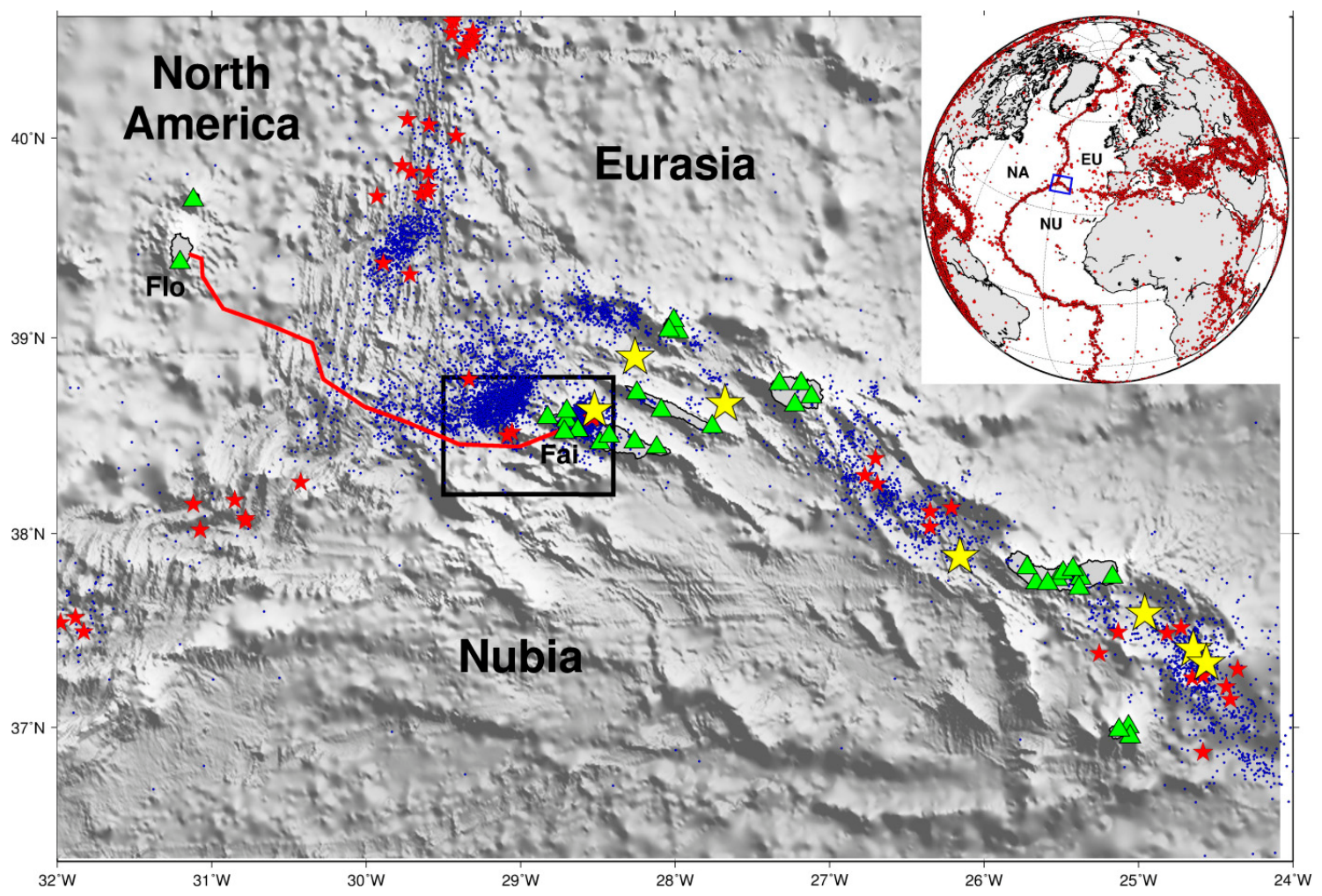
Figure 2.
Experiment setting in Faial, Azores. The approximate location of the monitored cable by HDAS is shown in thick white. The two OBS locations are shown in red circles. Green triangles show the land stations. Seismicity is shown as in Figure 1. The yellow star is the epicenter of the 9th July 1998 earthquake (ML = 5.8). The OBS is shown in the inset.
Figure 2.
Experiment setting in Faial, Azores. The approximate location of the monitored cable by HDAS is shown in thick white. The two OBS locations are shown in red circles. Green triangles show the land stations. Seismicity is shown as in Figure 1. The yellow star is the epicenter of the 9th July 1998 earthquake (ML = 5.8). The OBS is shown in the inset.
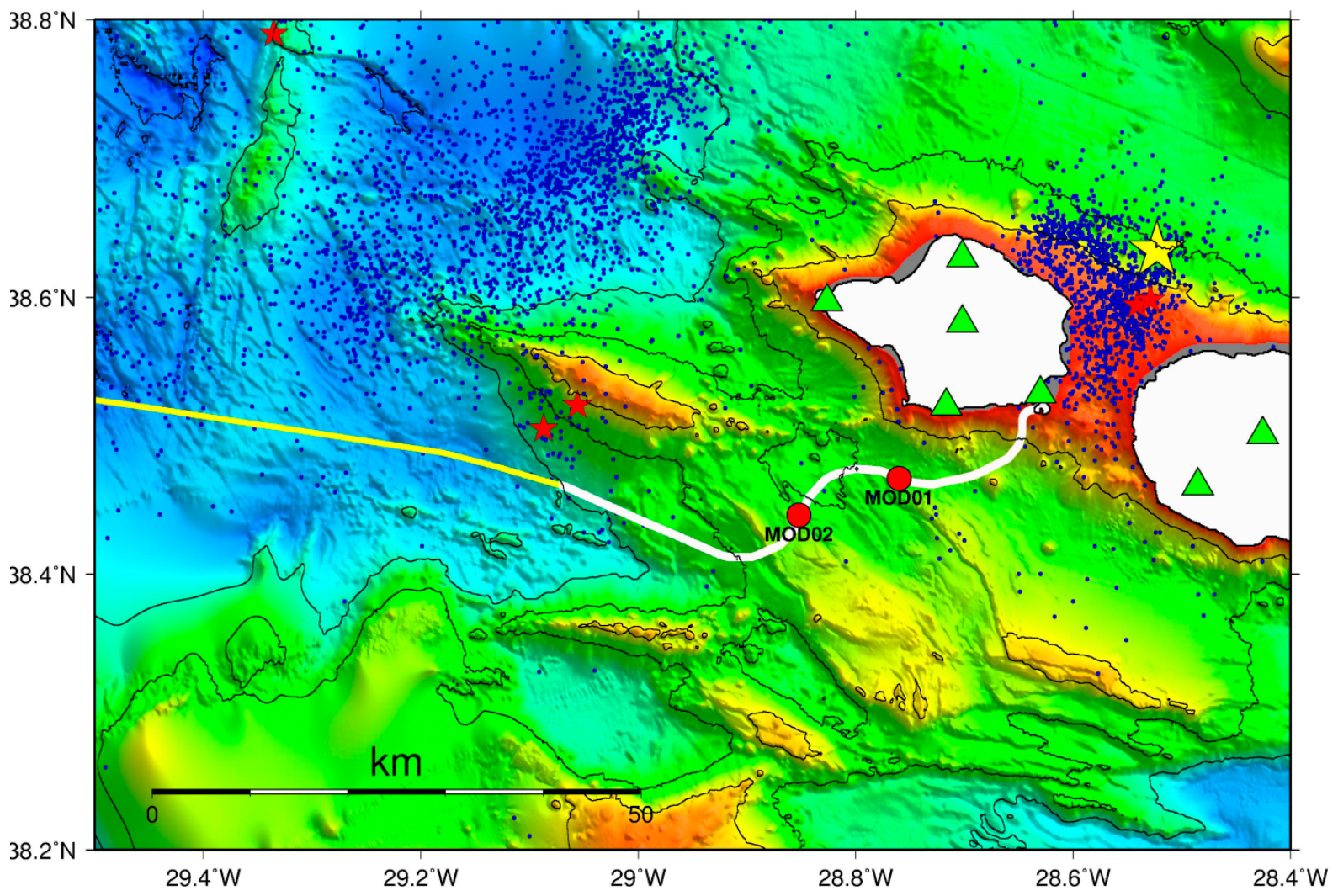
Figure 3.
(a) RMS computed for the whole cable monitored by HDAS. 4 domains can be identified as explained in the text. (b) Cable depth profile.
Figure 3.
(a) RMS computed for the whole cable monitored by HDAS. 4 domains can be identified as explained in the text. (b) Cable depth profile.
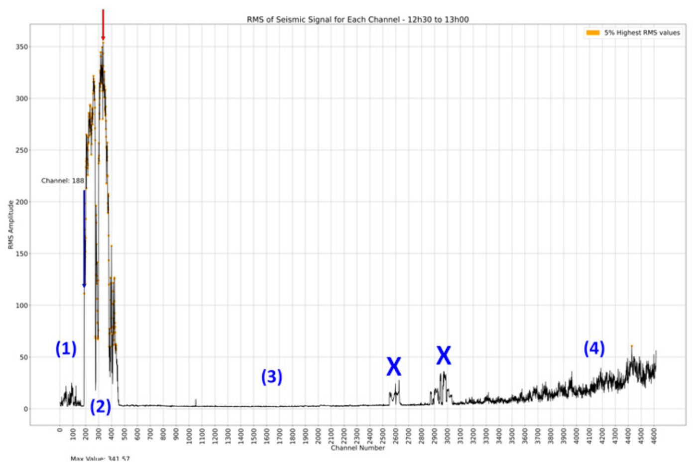
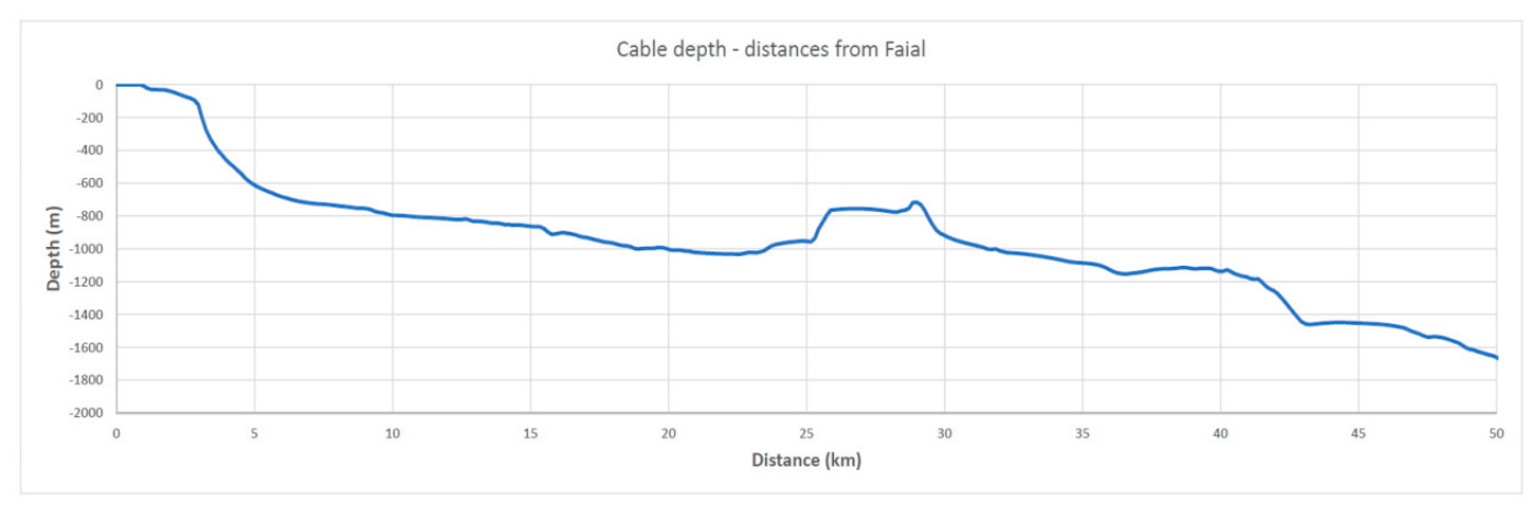
Figure 4.
PSD analysis for channel 1498 on the near deep water section (3). It shows an increase in 1/f noise at frequencies below 1 Hz.
Figure 4.
PSD analysis for channel 1498 on the near deep water section (3). It shows an increase in 1/f noise at frequencies below 1 Hz.
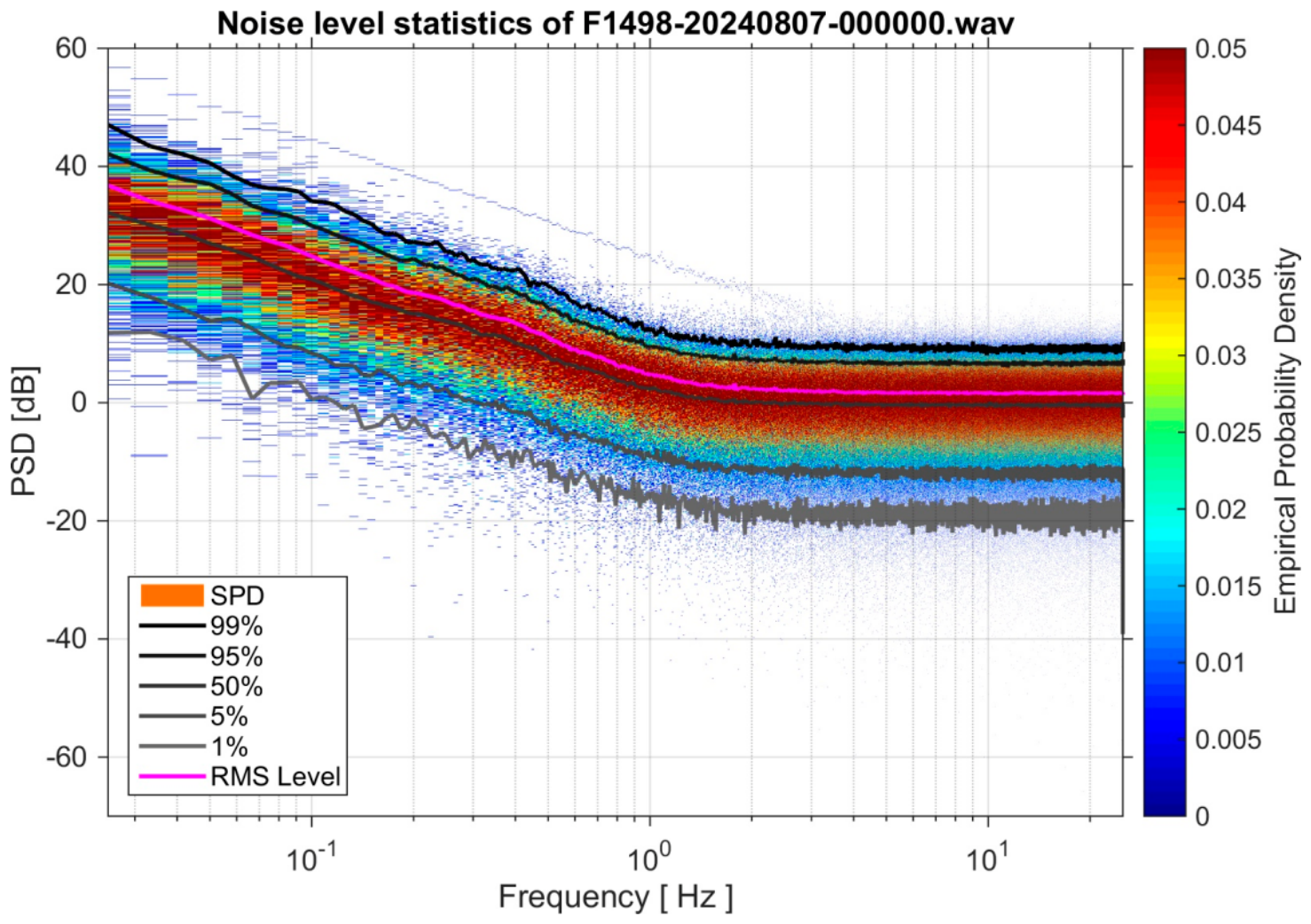
Figure 5.
Waveforms for 300 channels (spanning 3 km) recorded by HDAS close to MODAS OBS. Horizontal arrow show the orientation of offset axis and vertical arrow sows the orientation of the time axis.
Figure 5.
Waveforms for 300 channels (spanning 3 km) recorded by HDAS close to MODAS OBS. Horizontal arrow show the orientation of offset axis and vertical arrow sows the orientation of the time axis.
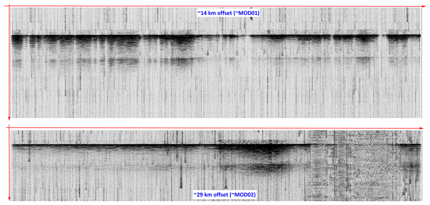
Figure 6.
Magnitude vs. distance for events recorded by HDAS as a function of quality. The black line is the inferred land network detectability.
Figure 6.
Magnitude vs. distance for events recorded by HDAS as a function of quality. The black line is the inferred land network detectability.
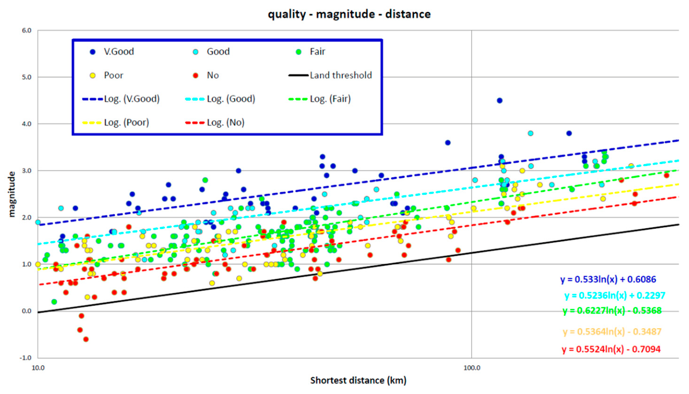
Figure 7.
Example of the choice of channels to be used for earthquake analysis based on the maximum S/N inside a few 100 m bins around each km mark.
Figure 7.
Example of the choice of channels to be used for earthquake analysis based on the maximum S/N inside a few 100 m bins around each km mark.
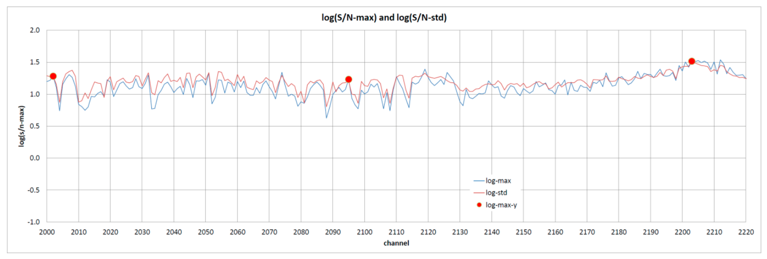
Figure 8.
Number of phases picked for the set of 31 events analyzed. (a) IPMA land stations. (b) HDAS channels. The numbers refer to the domains identified in Section 4.
Figure 8.
Number of phases picked for the set of 31 events analyzed. (a) IPMA land stations. (b) HDAS channels. The numbers refer to the domains identified in Section 4.
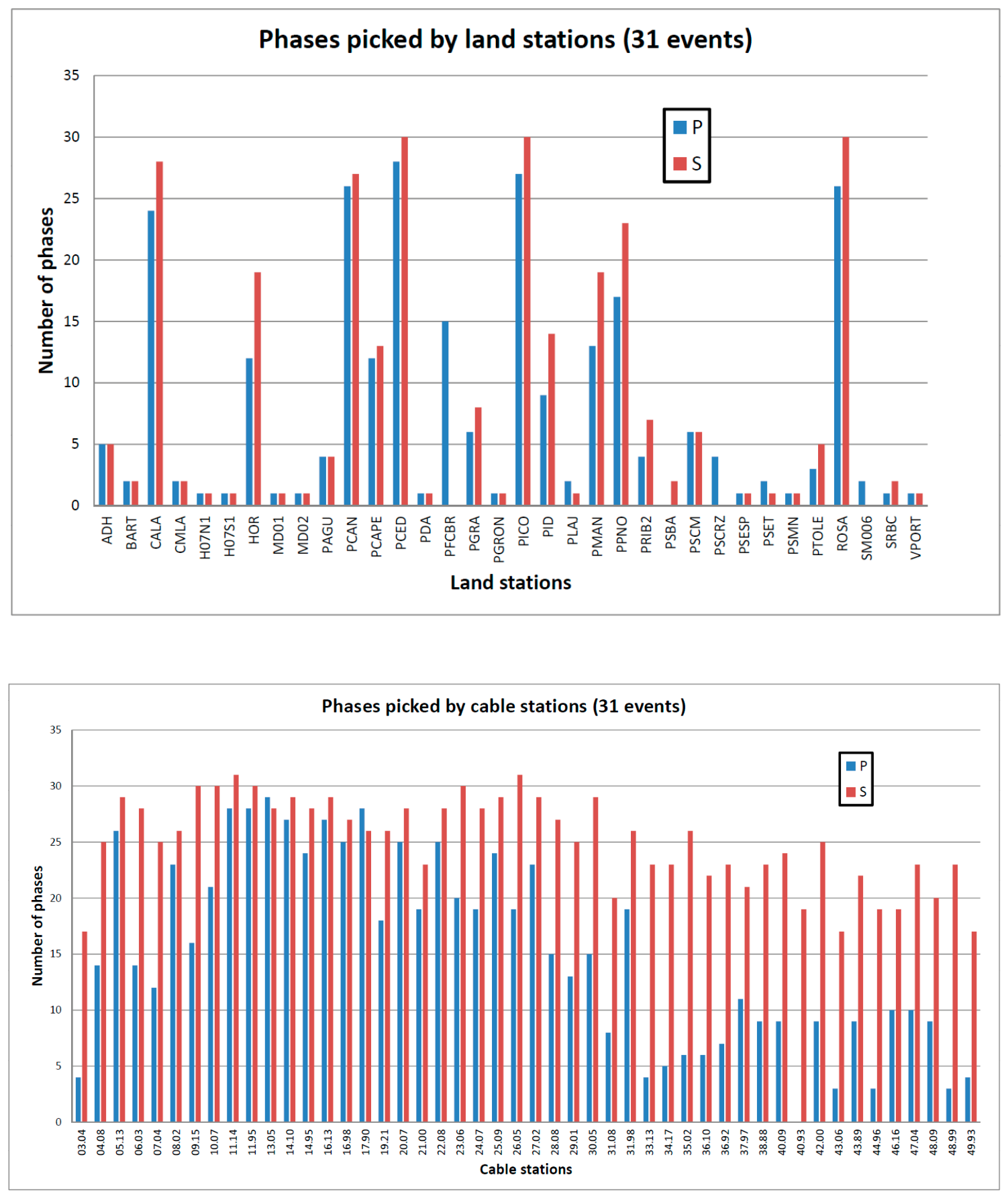
Figure 9.
Comparison of error ellipse areas. (a) between LOC00 (IPMA only) and LOC01 (IPMA + HDAS P & S). (b) between LOC00 and LOC02 (IPMA + HDAS S).
Figure 9.
Comparison of error ellipse areas. (a) between LOC00 (IPMA only) and LOC01 (IPMA + HDAS P & S). (b) between LOC00 and LOC02 (IPMA + HDAS S).
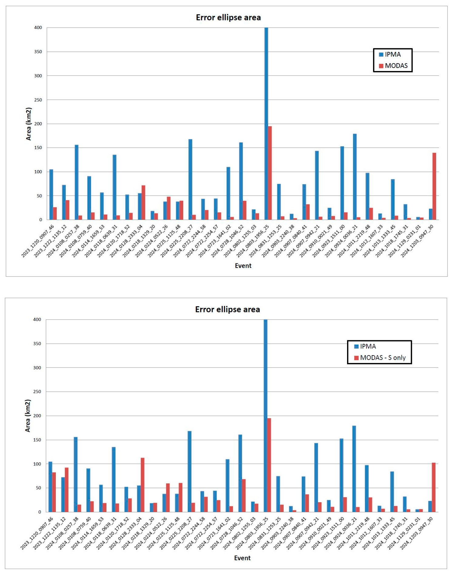
Figure 10.
Variation of error ellipse area (in %) between the original IPMA locations and the ones obtained adding HDAS P & S picks.
Figure 10.
Variation of error ellipse area (in %) between the original IPMA locations and the ones obtained adding HDAS P & S picks.
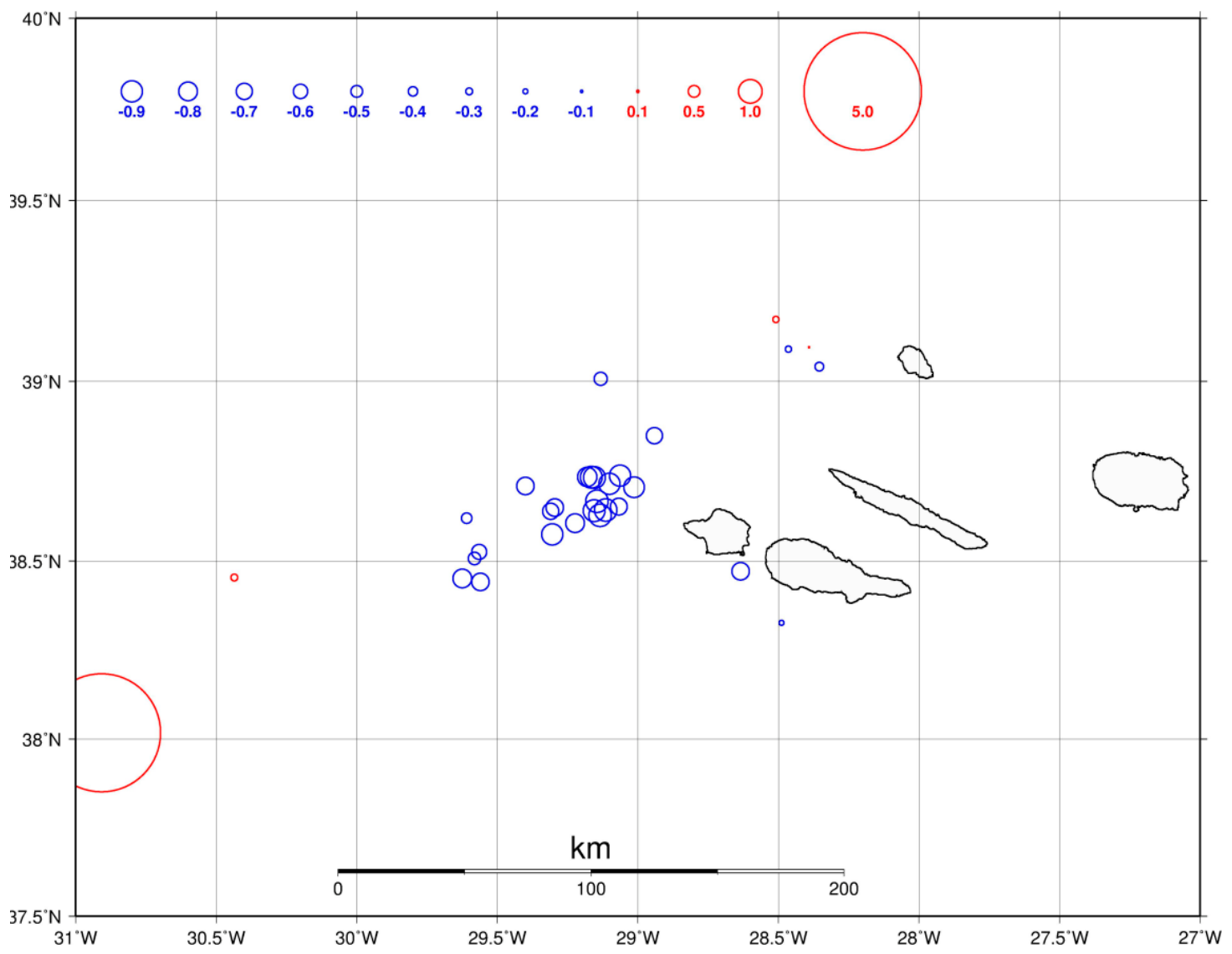
Figure 11.
Variation of depth error (in km) between the original IPMA locations and the ones obtained adding HDAS P & S picks.
Figure 11.
Variation of depth error (in km) between the original IPMA locations and the ones obtained adding HDAS P & S picks.
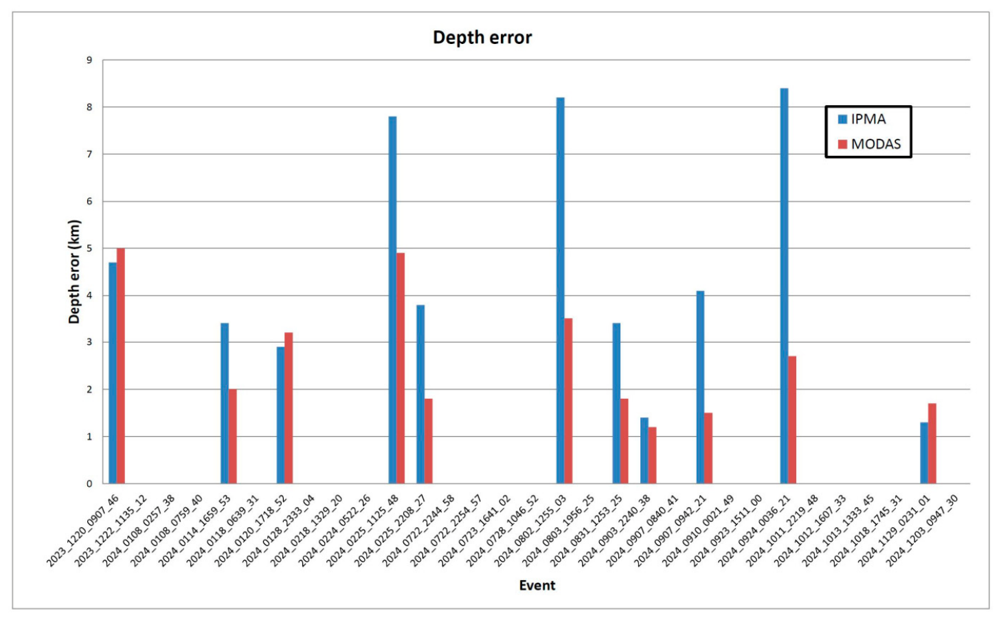
Figure 12.
Variation of error ellipse area (in %) between the original IPMA locations and the ones obtained adding HDAS P & S picks overlying the gap reduction between IPMA and IPMA + HDAS networks. Epicenters shown as in Figure 10.
Figure 12.
Variation of error ellipse area (in %) between the original IPMA locations and the ones obtained adding HDAS P & S picks overlying the gap reduction between IPMA and IPMA + HDAS networks. Epicenters shown as in Figure 10.
Disclaimer/Publisher’s Note: The statements, opinions and data contained in all publications are solely those of the individual author(s) and contributor(s) and not of MDPI and/or the editor(s). MDPI and/or the editor(s) disclaim responsibility for any injury to people or property resulting from any ideas, methods, instructions or products referred to in the content. |
© 2026 by the authors. Licensee MDPI, Basel, Switzerland. This article is an open access article distributed under the terms and conditions of the Creative Commons Attribution (CC BY) license (http://creativecommons.org/licenses/by/4.0/).
Copyright: This open access article is published under a Creative Commons CC BY 4.0 license, which permit the free download, distribution, and reuse, provided that the author and preprint are cited in any reuse.