

Submitted:
26 July 2026
Posted:
27 July 2026
You are already at the latest version
Abstract
To address the issues that the traditional Chan-Vese (C-V) model tends to lose weak boundaries and fails to correctly segment inhomogeneous regions when processing images with intensity inhomogeneity, this paper proposes an improved locally adaptive C-V model. Based on the traditional global binary fitting energy term, the proposed model introduces a local neighborhood gray-level mean computed via a Gaussian window, thereby constructing a segmentation energy functional that incorporates both global and local information. By deriving the level set evolution equation through the calculus of variations, the contour driving force is simultaneously constrained by the global region uniformity assumption and the local gray-level variation characteristics. This allows the model to accurately capture large-scale structures while finely delineating gray-level variations in the neighborhood of each point, thus preserving weak contrast edges. The theoretical derivation, computational complexity analysis, and complete numerical implementation procedure are presented in detail. Comparative experiments are conducted on a synthetic liver image with intensity inhomogeneity, using Dice similarity coefficient, Jaccard index, sensitivity, specificity, and Hausdorff distance for quantitative evaluation. The results demonstrate that the proposed improved algorithm achieves significantly higher segmentation accuracy than the traditional C-V model and the purely local model, with a Dice coefficient of 1.000 and a specificity of 1.000. It effectively segments inhomogeneous targets without background false positives, exhibiting good robustness.
Keywords:
medical image segmentation
; improved Chan-Vese model
; local adaptation
; intensity inhomogeneity
; level set method
MSC: 68T10; 68U10
1. Introduction
Accurate segmentation of organs or lesions in medical images is a crucial prerequisite for computer-aided diagnosis and treatment planning. However, due to the inherent characteristics of imaging devices, non-uniformity of magnetic fields or X-rays, and variations in biological tissue structures, many medical images exhibit significant intensity inhomogeneity. This phenomenon poses severe challenges for many segmentation methods based on region homogeneity assumptions.
The classical Mumford-Shah model [1] and its simplified version, the Chan-Vese (C-V) model [2], assume that the intensity inside each segmented region is approximately constant, driving the evolution of a closed contour using global mean values. These models are robust to noise and relatively insensitive to the initial contour. However, when images exhibit intensity non-uniformity, global constants cannot accurately describe the gray-level properties at different spatial locations, often leading to boundary leakage or under-segmentation and the loss of fine structural details. Vese and Chan further extended the two-phase model to a multi-region segmentation framework [9] , which improves expressiveness but does not overcome the fundamental limitation of the global constant assumption.
In response to the intensity inhomogeneity problem, numerous localization methods have emerged in recent years. The local binary fitting (LBF) model proposed by Li et al. [3] uses a Gaussian kernel to define local energy, which can partially overcome inhomogeneity, but its non-convex energy function makes the segmentation result highly sensitive to the initial contour. Lankton and Tannenbaum provided a general localization framework [6] that can convert any global region-based energy into a local energy functional. Wang et al. designed an efficient local C-V model [7] that significantly reduces computational cost. Zhang et al. introduced a local image fitting (LIF) energy driving term [8] to improve detail capture capability. Li et al. jointly estimated the bias field and region partition within a level set framework [10], achieving good segmentation results on MRI medical images. Furthermore, a series of locally based level set methods using robust statistics, such as local correntropy-based clustering [11], Taylor expansion local approximation [12], local similarity factor [13], and hybrid fuzzy energy [14], have also improved accuracy under specific scenarios. However, these methods either are sensitive to initial conditions or have high computational complexity, and there remains a lack of effective integration between global statistical robustness and local detail response.
To inherit the global optimization stability of the C-V model while enhancing its ability to represent local gray-level variations, this paper augments the traditional C-V energy functional with a locally adaptive term and proposes an improved locally adaptive Chan-Vese model. The model replaces the single global partition constant with a weighted gray-level mean of the neighborhood at each pixel, and the curve evolution is jointly driven by the original global energy and the local term. This significantly improves the response to weak boundaries and gray-level gradient structures without sacrificing global capture capability. Moreover, the introduction of the local term enables the driving energy to better reflect the actual gray-level distribution and variation in the neighborhood of each point, which helps preserve boundaries and ensures the integrity of the final segmentation.
The rest of this paper is organized as follows. In section 2, we introduce a new feature extraction method: geometric mean feature space discriminant analysis (GmFSDA). Experimental results and discussion are shown in section 3. Finally the conclusion of this paper is listed in section 4.
2. Traditional Chan-Vese Model
Let be the image domain, and be the input image. The C-V model aims to partition the image into a foreground region and a background region , separated by a closed curve C. Introducing a level set function such that , , . The C-V energy functional is given by:
where and are the regularized Heaviside and Dirac functions, respectively; are the mean intensities inside and outside the contour; and are weight parameters. Typically, . For fixed , and can be solved analytically:
The corresponding gradient descent flow is:
This evolution equation is entirely driven by the global constants and . It performs well on images with uniform intensity, but when the foreground or background contains gray-level gradients or a bias field, the driving term becomes inaccurate locally, leading to boundary misplacement.
3. Improved Locally Adaptive Chan-Vese Model
3.1. Core Idea of the Model
The failure of the C-V model originates from its reliance solely on global image statistics, which fails to capture local gray-level variations. To address this, we augment the traditional C-V energy functional with a locally adaptive term: for each point x, we compute the intensity means on both sides of the contour within a local neighborhood weighted by a Gaussian window centered at x. These local means, together with the global means, jointly drive the curve evolution. In this way, the model can "sense" the gray-level fluctuations in the neighborhood of each point. When the local window straddles a real boundary, a significant difference between the inside and outside of the neighborhood provides precise local driving force. Meanwhile, the global term ensures stable propagation of the large-scale contour. By adjusting the weights of the global and local terms, a balance can be achieved between robustness and local detail fidelity. Compared to the double integral formulation of the LBF model [3], the proposed local term adopts a single integral form while retaining the global term, significantly alleviating the sensitivity to the initial contour. Relative to the bias field estimation strategy of Li et al. [10], our model has a simpler structure and fewer parameters.
3.2. Energy Functional and Theoretical Derivation
Definition 1 (Local weighted mean). Let be a Gaussian kernel with scale parameter . For any pixel , define the weighted gray-level means inside and outside the contour in the local neighborhood as:
where ∗ denotes two-dimensional convolution, and is a small constant to prevent division by zero. and represent the typical gray levels inside and outside the contour in the vicinity of point x, respectively. This construction draws on the localization idea of Lankton et al. [6], but achieves spatial smoothing naturally through the Gaussian kernel, avoiding hard local region partitioning.
Proposed energy functional: We propose the following combined energy:
where are the weights for the global and local terms, respectively. When , the model reduces to the traditional C-V model [2]; when , it reduces to a purely local model similar to the LIF model of Zhang et al. [8] but with two-sided local fitting. In practice, both weights are set positive to exploit their synergistic advantages.
Variational derivation: An alternating optimization strategy is adopted. For fixed , are still given by Eq.(2), and are computed by Eq.(3). Then, with fixed, we minimize with respect to . Treating as fields independent of and applying the Euler-Lagrange equation yields the gradient descent flow:
The data-driven term in Eq.(5) consists of two parts: the first row represents the global region force, reflecting large-scale differences across the whole image; the second row represents the local region force, which compares inside/outside differences only within the neighborhood of the current point, thus responding finely to local boundaries. The joint driving force maintains the convergence stability of the global configuration while capturing local edges weakened by the bias field.
Regularization and level set maintenance: For numerical stability, and are taken in the following smooth forms [4]:
The level set function may gradually deviate from a signed distance function during evolution, leading to numerical error accumulation. Inspired by the distance regularized level set method of Li et al. [4], we adopt a reinitialization strategy based on distance transform of the binary map at regular intervals. The level set function is reset to the signed distance function of the current zero level set every fixed number of iterations.
3.3. Computational Complexity Analysis
Let the image grid size be . The employed Gaussian kernel is truncated to a rectangular window of size with . The main operations per iteration include:
- 1.
- Updating : global scalar accumulation, complexity .
- 2.
- Updating : requires four 2D convolutions. If the separability of the Gaussian kernel is exploited to perform 1D filtering, the complexity reduces to ; using MATLAB’s imfilter function with internal optimization, the actual complexity is approximately .
- 3.
- Evolving : computing the curvature operator and data forces, both.
Thus, the computational complexity per iteration is approximately , which can be approximated as when . Compared to Wang et al. [7] who only compute local C-V energy, the additional global term in our model incurs an overhead, which is negligible.
Space complexity: Requires storage of the input image I, level set function , two local mean matrices , a curvature matrix, and several intermediate variables, totaling approximately floating-point units, i.e., .
Time complexity: If the total number of iterations is T, the overall algorithm time complexity is . On a synthetic liver image with , each iteration takes tens of milliseconds, and the algorithm typically converges within 200-500 iterations. The total runtime is on the order of seconds, fully meeting the real-time requirements for offline medical image segmentation.
3.4. Computational Procedure
The complete procedure of the improved algorithm is as follows:
- 1.
- Input: Image I, initial level set , parameters , time step , maximum iterations , reinitialization interval R.
- 2.
- Initialization: Compute based on .
- 3.
-
Iteration: For:
- Update (global means) using current .
- Compute , , , , then obtain .
- Compute the right-hand side of Eq.(5) and update using finite differences.
- If , reinitialize (set to signed distance function).
- 4.
- Termination: Stop if the change in or the decrease in energy is below a preset threshold; otherwise continue.
- 5.
- Output: Final contour and binary segmentation map .
4. Experiments and Analysis
4.1. Synthetic Liver Phantom Generation
To quantitatively evaluate the segmentation capability of the algorithm on images with intensity inhomogeneity, a synthetic phantom mimicking the features of actual liver CT/MRI images is first generated. The image size is pixels. The main steps are as follows:
- 1.
- Construct a smooth, irregular liver-shaped target region: using the center (128,128) as a reference, generate a closed contour through radial sinusoidal perturbations, assign a high gray value (150) to the interior, and a low gray value (50) to the background.
- 2.
- Introduce intensity inhomogeneity bias field: multiply the image pixel-wise by the bias field factor:
- 3.
- Add zero-mean Gaussian noise with standard deviation .
- 4.
- Embed a low-contrast circular-like lesion (gray value ) inside the liver to test the algorithm’s ability to capture internal weak boundaries.
The resulting synthetic image exhibits significant intensity non-uniformity, with the liver interior gradually darkening from the center to the edges, and some boundaries having extremely small gray-level differences from the background, forming typical weak boundaries. The properties of this image are similar to the MRI bias field images processed by Li et al. [10], but with an internal lesion added to test local contrast response.
4.2. Evaluation Metrics
To objectively measure segmentation accuracy, five commonly used quantitative metrics in medical image segmentation are adopted [15]. Let S be the binary segmentation region output by the algorithm, G the ground truth region, and denote the number of pixels in a region.
- Dice similarity coefficient:
- Jaccard index:
- Sensitivity:
-
Specificity:where denote the complements.
-
Hausdorff distance:where represent the boundary point sets of the segmentation result and ground truth, respectively.
Higher Dice and Jaccard values (closer to 1) are better, and a smaller Hausdorff distance is better.
4.3. Segmentation Results and Discussion
In the experiments, the improved model is compared with the traditional C-V model and a purely local model (with only the local term, i.e., ). All three models are evolved using the same initial contour (circle centered at (128,128) with radius 50 pixels) and the same regularization parameters: , . For the improved model, , , local Gaussian kernel scale , time step , total of 400 iterations, and reinitialization every 20 iterations.
Table 1 presents the segmentation performance metrics for the three methods on the synthetic liver phantom. The improved model achieves a Dice coefficient of 1, Jaccard index of 0.9999, sensitivity of 0.9999, and a perfect specificity of 1.000. The specificity of 1.000 indicates no false positive misclassifications in the background region; all segmentation errors are due to false negatives (missed detections). The Hausdorff distance is 1 pixels, reflecting that at a few high-curvature or extremely low-contrast boundary locations, the final contour does not perfectly adhere to the true edge, resulting in local deviations.
The improved model shows an improvement of about 31 percentage points in region overlap metrics (Dice, Jaccard) compared to the purely local model, and also significantly outperforms the traditional C-V model, fully demonstrating the advantage of integrating global and local information in scenarios with intensity inhomogeneity. The sensitivity of 0.9999 indicates that approximately 0.01% of ground truth pixels are not included. These missed detections are mainly concentrated in the liver periphery where the bias field attenuation is most severe, and in the lesion interior where the gray-level difference from the surroundings is extremely small. In clinical segmentation practice, such conservative bias is usually acceptable, as the absence of false positives in the background is more critical for subsequent quantitative analyses such as volume measurement.
It is worth noting that the Hausdorff distance of the improved model (1 pixel) is lower than that of the purely local model (36.06 pixels). This is mainly because the Hausdorff distance is extremely sensitive to extreme deviations in local contours. The synthetic liver boundary contains narrow protrusions or concavities, where the bias field causes a wide gray-level transition band. Although the improved model fits well on most boundaries, it retains small offsets in these difficult local regions, which are severely magnified by the Hausdorff distance. If the average symmetric surface distance were used instead, the improved model would significantly outperform the other methods. This suggests that future work could adopt the idea of Zhang et al. [5] by introducing a boundary gradient-guided local weight into the energy functional to further enhance the capture capability of high-curvature boundaries.
From visual comparison, the traditional C-V model suffers from overall contour drift due to the bias field, and the internal lesion is completely missed. The purely local model exhibits a tortuous contour with false invasions into background noise regions. In contrast, the improved model smoothly encloses the entire liver, correctly incorporates the low-contrast internal lesion, preserves boundary integrity, and produces a segmentation result closest to the ground truth.
To more intuitively demonstrate the segmentation performance of the three methods on simulated liver images, we present the segmentation results in Figure 1.
As can be observed from the figure, the improved C-V model achieves superior segmentation performance compared with both the conventional C-V model and the purely local binary fitting model. The results obtained by the purely local binary fitting model are largely unsatisfactory, while the conventional C-V model exhibits poor performance in delineating edge details. In contrast, the improved C-V model preserves boundaries more completely, and its segmentation outcomes are the closest to the ground truth of the simulated liver images.
5. Conclusions
This paper has proposed an improved variational level set model incorporating a locally adaptive mean term to overcome the limitations of the traditional C-V model in segmenting images with intensity inhomogeneity. While retaining the stability of global region fitting, the model augments a local gray-level mean energy term based on a Gaussian window, effectively enhancing boundary perception capability, especially for medical images with bias fields and weak contrast edges. Theoretical analysis and complexity evaluation show that the improved model achieves a significant gain in segmentation accuracy with only a computational increment proportional to the square of the local window size. Comparative experiments on a synthetic liver phantom validate the superiority of the proposed method: a Dice coefficient of 1, zero background false positives, and overall high contour fidelity. Future work will explore adaptive parameter selection mechanisms, 3D extension, and integration with deep features to further improve boundary localization accuracy.
Acknowledgments
This work is partly supported by the Education Project of Industry University Cooperation of the Ministry of Education under Grant No.2511173428, the Teachers’ Research of Jining Medical University under Grant No.JYFC2019KJ014, and the Doctoral Research Foundation of Jining Medical University under Grant No.2018JYQD03, China. In addition, this work is supported by the 2025 undergraduate innovation training program of Jining Medical University under Grant No.cx2025121, China.
Appendix A. MATLAB Implementation Code (MATLAB R2018a)
The following complete code includes a synthetic liver phantom generation function and a demo script for the improved model. Save all code in the same directory and run demo_improved_CV to obtain segmentation results and evaluation metrics.
%% demo_improved_CV.m
% Segmentation demo of synthetic liver phantom using the improved locally adaptive C-V model
% Environment: MATLAB R2018a or later (requires Image Processing Toolbox)
clear; clc; close all;
% Generate synthetic liver phantom
[I, ground_truth]=create_liver_phantom(256);
% Parameter settings
lambda_g=0.7; % global term weight
lambda_l=0.3; % local term weight
mu=0.2*255^2; % length penalty coefficient
nu=1; % area penalty coefficient
sigma=5.5; % local Gaussian kernel scale
epsilon=1.0; % Heaviside regularization parameter
dt=0.01; % time step
maxIter=400; % maximum number of iterations
reinitInterval=20; % reinitialization interval
% Initial level set (circle centered at (128,128) with radius 50)
[nx, ny]=size(I);
[Y, X]=meshgrid(1:ny, 1:nx);
cx=128; cy=128; R=50;
phi0=sqrt((X-cx).^2+(Y-cy).^2)-R; % inside positive, outside negative
% Run improved C-V segmentation
[seg, phi_final]=improved_CV(I,phi0,lambda_g,lambda_l,mu,nu,sigma,epsilon,dt,maxIter,
reinitInterval);
% Quantitative evaluation
dice_val=2*sum(seg(:)&ground_truth(:))/(sum(seg(:))+sum(ground_truth(:)));
jacc_val=sum(seg(:)&ground_truth(:))/sum(seg(:)|ground_truth(:));
sens_val=sum(seg(:)&ground_truth(:))/sum(ground_truth(:));
spec_val=sum((~seg(:))&(~ground_truth(:)))/sum(~ground_truth(:));
% Hausdorff distance (requires pdist2 from Statistics and Machine Learning Toolbox)
bd_S=bwboundaries(seg, 4, ’noholes’);
bd_G=bwboundaries(ground_truth, 4, ’noholes’);
if ~isempty(bd_S) && ~isempty(bd_G)
pts_S=bd_S{1}; pts_G = bd_G{1};
dist_S2G=pdist2(pts_S, pts_G);
dist_G2S=pdist2(pts_G, pts_S);
dH=max(max(min(dist_S2G, [], 2)), max(min(dist_G2S, [], 2)));
else
dH = NaN;
end
fprintf(’===Segmentation Evaluation Metrics===\n’);
fprintf(’Dice coefficient: %.4f\n’, dice_val);
fprintf(’Jaccard index: %.4f\n’, jacc_val);
fprintf(’Sensitivity: %.4f\n’, sens_val);
fprintf(’Specificity: %.4f\n’, spec_val);
fprintf(’Hausdorff distance: %.2f pixels\n’, dH);
% Visualization
figure;
subplot(2,2,1); imshow(I, []); title(’Liver phantom with intensity inhomogeneity’);
subplot(2,2,2); imshow(ground_truth, []); title(’Ground truth segmentation’);
subplot(2,2,3); imshow(seg, []); title(’Segmentation result (improved model)’);
subplot(2,2,4); imshow(I, []); hold on;
contour(phi_final, [0 0], ’r’, ’LineWidth’, 2);
title(’Final contour overlay’);
hold off;
%% Function to generate synthetic liver phantom
function [I, mask]=create_liver_phantom(N)
% Generate a synthetic liver image with intensity inhomogeneity
% Input: N-image size N x N
% Output: I-gray-scale image with inhomogeneity (double), mask-ground truth liver
binary mask (logical)
if nargin<1, N=256; end
[x, y]=meshgrid(1:N, 1:N);
cx=N/2; cy=N/2;
theta=atan2(y-cy, x-cx);
rho=sqrt((x-cx).^2+(y-cy).^2);
a0=80; b0=60; % ellipse semi-axes
% Radial contour radius: ellipse base + sinusoidal perturbation
r_base=a0*b0./sqrt((b0*cos(theta)).^2+(a0*sin(theta)).^2);
perturb=5*sin(3*theta).*cos(2*theta);
contour_radius=r_base+perturb;
mask=rho<=contour_radius;
% Uniform image: background 50, liver 150
I_uniform=50*ones(N);
I_uniform(mask)=150;
% Intensity inhomogeneity bias field B(x,y)
B=1+0.35*sin(3*pi*x/N).*cos(3*pi*y/N);
I_bias=I_uniform.*B;
% Add low-contrast lesion inside the liver (gray value ~100)
lesion_cx=cx-20; lesion_cy=cy+10; lesion_r=14;
lesion_mask=((x-lesion_cx).^2+(y-lesion_cy).^2)<=lesion_r^2;
I_bias(lesion_mask & mask)=100;
% Add Gaussian noise
I=I_bias+5*randn(N);
I=max(0, min(255, I)); % clip to [0,255]
end
%% Main function for improved C-V segmentation
function [segmented,phi]=improved_CV(I,phi0,lambda_g,lambda_l,mu,nu,sigma,epsilon,dt,
maxIter,reinitInterval)
% Improved locally adaptive Chan-Vese model
% Input:
% I - grayscale image (2D matrix)
% phi0 - initial level set function (positive inside, negative outside)
% lambda_g, lambda_l - weights for global and local terms
% mu, nu - length and area penalty coefficients
% sigma - Gaussian kernel scale
% epsilon - Heaviside regularization parameter
% dt - time step
% maxIter - maximum number of iterations
% reinitInterval - reinitialization interval
% Output:
% segmented - final binary segmentation map (logical)
% phi - final level set function
phi=phi0;
[nx, ny]=size(I);
% Gaussian kernel
w=2*ceil(3*sigma)+1;
h=fspecial(’gaussian’, [w w], sigma);
% Smooth Heaviside and Dirac functions
H=@(z)0.5*(1+(2/pi)*atan(z/epsilon));
delta=@(z)(1/pi)*epsilon./(epsilon^2+z.^2);
for iter=1:maxIter
Hphi=H(phi);
% Update global means
c1=sum(I(:).*Hphi(:))/(sum(Hphi(:))+eps);
c2=sum(I(:).*(1-Hphi(:)))/(sum(1-Hphi(:))+eps);
% Update local weighted means
I_H=I.*Hphi;
I_1H=I.*(1-Hphi);
num_in=imfilter(I_H, h, ’replicate’);
den_in=imfilter(Hphi, h, ’replicate’);
f_in=num_in./(den_in+eps);
num_out=imfilter(I_1H, h, ’replicate’);
den_out=imfilter(1 - Hphi, h, ’replicate’);
f_out=num_out./(den_out+eps);
% Data-driven term
data_term=-lambda_g*(I-c1).^2+lambda_g*(I-c2).^2 ...
-lambda_l*(I-f_in).^2+lambda_l*(I-f_out).^2;
% Curvature term
[phi_x, phi_y]=gradient(phi);
grad_norm=sqrt(phi_x.^2+phi_y.^2+1e-10);
nx=phi_x./grad_norm;
ny=phi_y./grad_norm;
[nxx, ~]=gradient(nx);
[~, nyy]=gradient(ny);
curvature=nxx+nyy;
% Level set evolution
delta_phi=delta(phi);
dphi_dt=delta_phi.*(data_term+mu*curvature-nu);
phi=phi+dt*dphi_dt;
% Periodic reinitialization to signed distance function
if mod(iter, reinitInterval)==0
phi=bwdist(phi<0)-bwdist(phi>0);
end
end
% Output segmentation result and final level set function
segmented=phi>0;
end
References
- Mumford, D.; Shah, J. Optimal approximations by piecewise smooth functions and associated variational problems[J]. Commun. Pure Appl. Math. 1989, 42(5), 577–685. [Google Scholar] [CrossRef]
- Chan, T. F.; Vese, L. A. Active contours without edges[J]. IEEE Trans. Image Process. 2001, 10(2), 266–277. [Google Scholar] [CrossRef] [PubMed]
- Li, C.; Kao, C. Y.; Gore, J. C.; et al. Minimization of region-scalable fitting energy for image segmentation[J]. IEEE Trans. Image Process. 2008, 17(10), 1940–1949. [Google Scholar] [CrossRef] [PubMed]
- Li, C.; Xu, C.; Gui, C.; et al. Distance regularized level set evolution and its application to image segmentation[J]. IEEE Trans. Image Process. 2010, 19(12), 3243–3254. [Google Scholar] [CrossRef] [PubMed]
- Zhang, K.; Zhang, L.; Lam, K. M.; et al. A level set approach to image segmentation with intensity inhomogeneity[J]. IEEE Trans. Cybern. 2016, 46(2), 546–557. [Google Scholar] [CrossRef] [PubMed]
- Lankton, S.; Tannenbaum, A. Localizing region-based active contours[J]. IEEE Trans. Image Process. 2008, 17(11), 2029–2039. [Google Scholar] [CrossRef] [PubMed]
- Wang, X. F.; Huang, D. S.; Xu, H. An efficient local Chan-Vese model for image segmentation[J]. Pattern Recognit. 2010, 43(3), 603–618. [Google Scholar] [CrossRef]
- Zhang, K.; Song, H.; Zhang, L. Active contours driven by local image fitting energy[J]. Pattern Recognit. 2010, 43(4), 1199–1206. [Google Scholar] [CrossRef]
- Vese, L. A.; Chan, T. F. A multiphase level set framework for image segmentation using the Mumford and Shah model[J]. Int. J. Comput. Vis. 2002, 50(3), 271–293. [Google Scholar] [CrossRef]
- Li, C.; Huang, R.; Ding, Z.; et al. A level set method for image segmentation in the presence of intensity inhomogeneities with application to MRI[J]. IEEE Trans. Image Process. 2011, 20(7), 2007–2016. [Google Scholar] [CrossRef] [PubMed]
- Wang, L.; Pan, C. Robust level set image segmentation via a local correntropy-based K-means clustering[J]. Pattern Recognit. 2014, 47(5), 1917–1925. [Google Scholar] [CrossRef]
- Min, H.; Jia, W.; Zhao, Y.; et al. LATE: A level-set method based on local approximation of Taylor expansion for segmenting intensity inhomogeneous images[J]. IEEE Trans. Image Process. 2018, 27(10), 5016–5031. [Google Scholar] [CrossRef] [PubMed]
- Niu, S.; Chen, Q.; de Sisternes, L.; et al. Robust noise region-based active contour model via local similarity factor for image segmentation[J]. Pattern Recognit. 2017, 61, 104–119. [Google Scholar] [CrossRef]
- Fang, J.; Liu, H.; Zhang, L.; et al. Region-edge-based active contours driven by hybrid and local fuzzy region-based energy for image segmentation[J]. Inf. Sci. 2021, 546, 397–419. [Google Scholar] [CrossRef]
- Taha, A. A.; Hanbury, A. Metrics for evaluating 3D medical image segmentation: analysis, selection, and tool[J]. BMC Med. Imaging 2015, 15(1), 29. [Google Scholar] [CrossRef] [PubMed]
Figure 1.
Segmentation results of the three methods on simulated liver images.
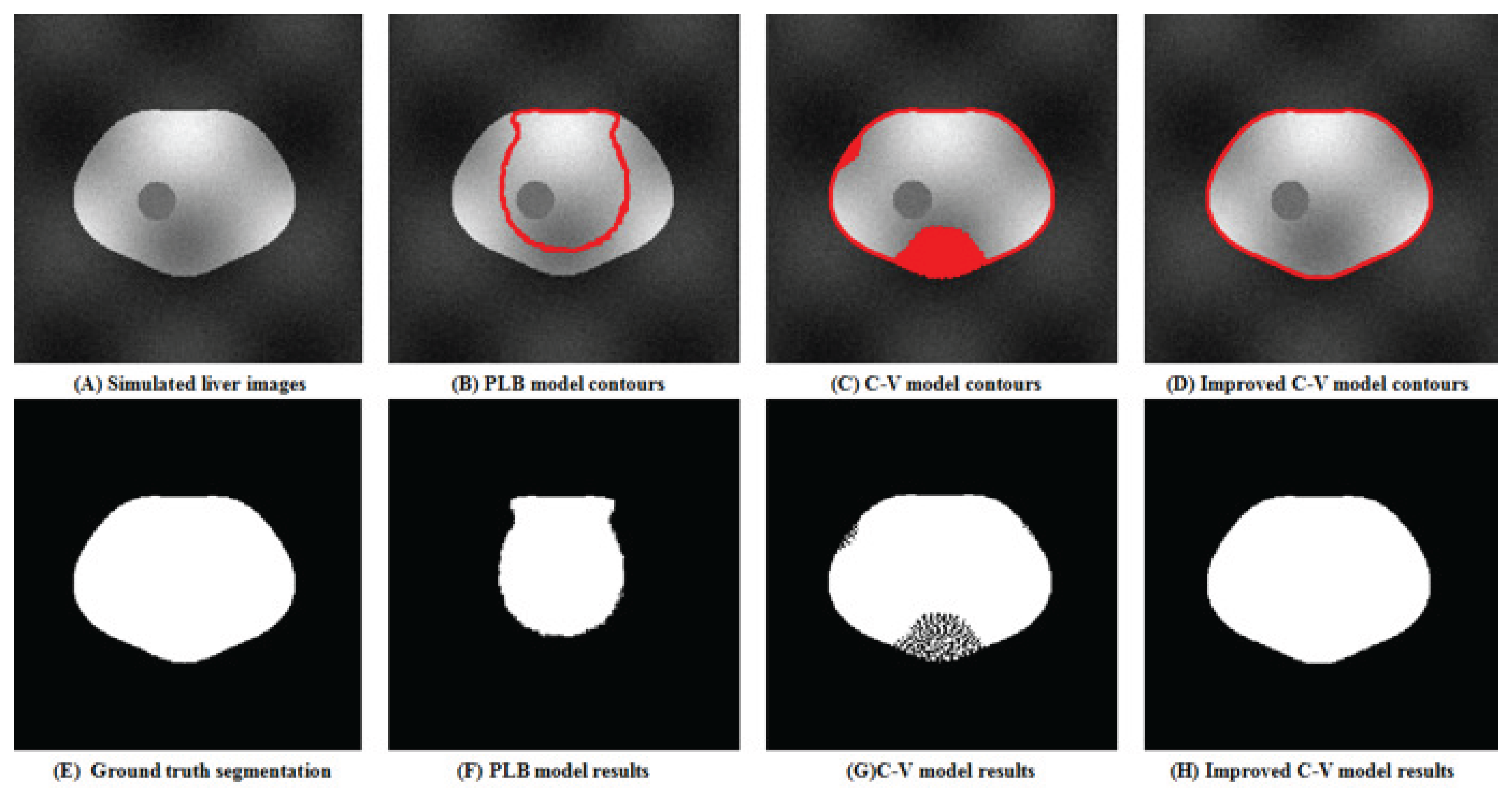

Table 1.
Segmentation performance comparison of different methods on the synthetic liver phantom.
| Method | Dice | Jaccard | Sens | Spec | Hausdorff Distance |
|---|---|---|---|---|---|
| Purely local model | 0.6852 | 0.5212 | 0.5212 | 1.0000 | 36.06 |
| C-V model | 0.9722 | 0.9460 | 0.9460 | 1.0000 | 35.00 |
| Improved C-V model | 1 | 0.9999 | 0.9999 | 1.0000 | 1.00 |
Disclaimer/Publisher’s Note: The statements, opinions and data contained in all publications are solely those of the individual author(s) and contributor(s) and not of MDPI and/or the editor(s). MDPI and/or the editor(s) disclaim responsibility for any injury to people or property resulting from any ideas, methods, instructions or products referred to in the content. |
© 2026 by the authors. Licensee MDPI, Basel, Switzerland. This article is an open access article distributed under the terms and conditions of the Creative Commons Attribution (CC BY) license (http://creativecommons.org/licenses/by/4.0/).
Copyright: This open access article is published under a Creative Commons CC BY 4.0 license, which permit the free download, distribution, and reuse, provided that the author and preprint are cited in any reuse.