

Submitted:
24 July 2026
Posted:
27 July 2026
You are already at the latest version
Abstract
Accurate measurement and forecasting of inflation expectations are essential for sustaining financial stability and supporting effective economic decision-making. Conventional forecasting approaches rely predominantly on survey-based expectations and low-frequency macroeconomic indicators, which are subject to publication delays and have limited responsiveness to rapidly shifting economic conditions. To address this challenge, a novel inflation nowcasting framework is proposed that integrates expectations from a survey of market participants conducted by the Central Bank of the Republic of Türkiye with high-frequency search query data from Google Trends. By capturing real-time shifts in consumer attention and behavior, the proposed framework reduces the information gap that occurs prior to the publication of official statistics. The forecasting model is developed using AutoTS, an automated machine learning (AutoML) framework that remains relatively unexplored in the inflation forecasting literature. Empirical evaluations demonstrate that the presented methodology reduces forecast errors by 32.99% relative to survey-based expectations, achieving an out-of-sample symmetric mean absolute percentage error of 18.18%. A main advantage of the model is its adaptability to structural breaks and regime shifts in inflation patterns. For example, at a monthly inflation rate of 4.84% in January 2026, the absolute forecast error is limited to 0.22 percentage points, compared to 1.08 percentage points for expert forecasts. Similarly, for a disinflationary episode in November 2025, with monthly inflation declining to 0.87%, an estimate of 0.95% is generated, thereby mitigating the adjustment lag commonly associated with conventional expert-based expectations. These results indicate that search query data possess meaningful incremental predictive value that is not completely captured by traditional surveys. Consequently, integrating high-frequency behavioral signals with expert expectations through an AutoML framework improves the timeliness and accuracy of inflation nowcasts, particularly during periods of heightened volatility and rapid regime shifts.
Keywords:
nowcasting
; information asymmetry
; Google search query data
; survey of market participants
; AutoML
; AutoTS
1. Introduction
Inflation forecasting remains a central focus in economic research, with ongoing efforts to enhance predictive accuracy by integrating novel data sources and analytical methods. Traditional forecasting approaches predominantly utilize survey-based expectations and macroeconomic indicators to explain price dynamics [1,2]. Although these sources are valuable, their relatively low publication frequency and susceptibility to reporting delays and revisions introduce a structural information lag, thereby constraining their utility for real-time economic assessment and policy formulation [3].
In response to these limitations, recent studies have increasingly explored alternative data sources derived from digital activity. Among these, Google search query data (GSQD) have emerged as a valuable resource capturing real-time consumer attention, expectations, and behavioral responses to economic developments [4]. Unlike conventional macroeconomic indicators, GSQD are generated continuously and are available without publication delays, making this type of data an effective high-frequency proxy for current economic conditions [5,6].
The increasing use of GSQD has supported the development of more sophisticated forecasting frameworks. Integrating GSQD with traditional economic variables has enabled the application of advanced methodologies, such as mixed-frequency models, dynamic variable selection techniques, and real-time data assimilation [7]. Beyond timeliness, search query data provide practical advantages including low acquisition costs, immediate availability, and immunity to subsequent revisions. Although challenges related to noise and sample representativeness persist, empirical studies consistently show that GSQD can achieve forecasting performance comparable to or surpassing that of traditional indicators [8,9].
A substantial body of empirical evidence demonstrates the effectiveness of GSQD in inflation forecasting. Studies that combine high-frequency search data with conventional macroeconomic indicators report significant improvements in predictive accuracy. For example, one study achieved a 32.9% reduction in root mean square error (RMSE) when forecasting the Chinese Consumer Price Index (CPI), underscoring the strong relationship between search behavior and official inflation statistics [10]. The success of these models depends significantly on keyword selection and data processing methodologies. The Google Inflation Search Index (GISI), developed using artificial intelligence and web-scraping techniques, has shown superior forecasting performance compared to traditional survey-based expectations, particularly for medium-term inflation forecasts [11].
The advantages of GSQD are also apparent when they are integrated into classical econometric frameworks. Research indicates that augmenting autoregressive integrated moving average (ARIMA) models with search query data significantly enhances forecasting performance, particularly during periods of elevated inflation and economic uncertainty [12]. Similarly, dynamic model averaging approaches demonstrate that search data offer valuable predictive information in both developed and emerging economies, although model effectiveness depends in part on data quality and sample size [13].
Cross-country analyses further substantiate these findings. Research employing methodologies such as panel vector autoregression and mixed data sampling has identified robust dynamic relationships between search intensity and inflation indicators, particularly within emerging markets [14]. Country-specific studies, including those conducted in Morocco, show that incorporating GSQD-based indices into seasonal ARIMA models enhances forecast accuracy and improves the modeling of inflation uncertainty in rapidly evolving economic environments [15].
Beyond forecasting applications, GSQD also contribute to the analysis of informational frictions within the economy. Comparative studies of search activity and traditional information sources, such as newspaper coverage, indicate that digital search behavior reveals informational rigidities not fully captured by conventional indicators [16]. Additionally, research employing the hybrid new Keynesian Phillips curve framework has shown that internet-based expectations derived from GSQD outperform both traditional time-series models and survey-based inflation expectations [17].
Further evidence indicates that GSQD-based inflation expectations exhibit characteristics consistent with rational expectations and provide valuable insight into consumer behavior [18]. Moreover, hybrid models that combine lagged inflation measures with search query variables consistently yield lower forecast errors than models relying solely on traditional indicators [19].
Advancements in machine learning and deep learning techniques have broadened the potential applications of GSQD in inflation forecasting. Artificial intelligence-driven frameworks, including GISI-based models and deep neural networks, demonstrate strong capabilities in capturing forward-looking inflation dynamics and improving predictive accuracy [20,21]. Furthermore, two-stage machine learning models that utilize extensive feature sets and regularization techniques such as Lasso and Ridge regression enable more granular and timely detection of inflationary pressures. These approaches are particularly valuable in data-constrained environments, where they may serve as effective early-warning systems for policymakers [22].
In summary, the literature demonstrates that integrating high-frequency search query data with traditional macroeconomic indicators can substantially improve inflation forecasting performance. By overcoming the limitations of publication delays and low-frequency data, GSQD constitute a timely, scalable, and increasingly reliable information source. When combined with advanced econometric and machine learning methodologies, these digital signals serve as a powerful tool for analyzing inflation dynamics and supporting more informed economic decision-making.
2. Problem Definition
The survey of market participants conducted monthly by the Central Bank of the Republic of Türkiye (TCMB) assesses forward-looking expectations among experts and decision-makers in the financial and real sectors. Responses are gathered over a short period in the second or third week of each month and are typically published within two business days, providing a timely benchmark for expectations prior to the release of official inflation figures [23]. In contrast to consumer tendency surveys, which generally emphasize year-end inflation expectations, this survey of market participants provides direct estimates of current month-end inflation, enhancing its utility for nowcasting. While the number of respondents fluctuates, the survey consistently represents the perspectives of a highly informed group of market participants. For example, there were 56 participants in July 2021 and 67 in March 2026 [23,24]. Consequently, the survey serves not only as a statistical measure but also as a proxy for expert consensus regarding future inflation developments.
Despite its strengths, the survey also has several important limitations. Although it is forward-looking, participants formulate their expectations based on information available at the time of the survey, rendering forecasts vulnerable to rapidly changing economic conditions and information lag. The relatively small, non-random sample may further limit representativeness, as responses predominantly reflect the perspectives of financial and corporate professionals rather than the general population. Behavioral factors such as anchoring, herding effects, and strategic forecasting may also influence expectations and reduce forecast efficiency. Moreover, the fixed monthly survey window restricts the integration of intra-month developments, and the lack of high-frequency updates limits responsiveness to unforeseen economic shocks. Consequently, while the survey provides valuable expert-based insights, it may not fully capture real-time changes in inflation expectations.
In contrast, GSQD offer a high-frequency, behavior-based data source that captures consumers’ real-time responses to economic developments. Given that perceptions of price changes are fundamental to inflation dynamics, online search activity presents a unique opportunity for observing evolving expectations and concerns as they emerge. Search terms associated with inflationary pressures, such as “price increase,” “price hike,” “discount,” and “cheapest,” may act as early indicators of changes in consumer sentiment, demand conditions, and inflation expectations. Therefore, GSQD can capture micro-level behavioral dynamics largely absent in the outcomes of traditional survey-based approaches.
This study argues that integrating GSQD with the TCMB’s survey of market participants creates a complementary forecasting framework that utilizes the strengths of both data sources. The survey captures the rational expectations of informed market participants, while search query data provide real-time behavioral signals from consumers. Combining these datasets is expected to reduce information gaps ahead of the release of official inflation statistics and enhance the timeliness of inflation forecasts. Additionally, the joint use of expert expectations and digital behavioral data may improve forecasting accuracy and provide deeper insight into forecast errors and their underlying causes.
Accordingly, the primary objective of this study is to develop and assess a novel inflation nowcasting framework that integrates traditional expectation-based indicators with high-frequency behavioral data. Specifically, the study examines whether GSQD function solely as complementary variables or serve as leading indicators that can systematically improve inflation-forecasting performance. By jointly modeling results from surveys of market participants and search volume indicators, this study aims to enhance forecasting accuracy, timeliness, and bias mitigation.
This study contributes to the emerging literature on the integration of expert expectations with behavioral big data. In addition to proposing a technical forecasting model, it seeks to establish a broader conceptual framework for understanding inflation dynamics by leveraging the interaction between rational expectations and real-time digital behavior. This approach provides new insight into how high-frequency information can complement traditional economic indicators and enhance the monitoring of inflationary developments.
Drawing on the theoretical and empirical literature summarized above, the following hypotheses are tested:
H1: Google search query data contain statistically significant predictive information regarding future inflation.
H2: Combining Google search query data with survey-based market expectations improves inflation forecasting performance compared to using survey-based forecasts alone.
H3: The forecasting gains from Google search query data are more pronounced during periods of elevated inflation volatility.
3. Methodology
In line with the objective of the study as outlined above, the process flow presented in Figure 1 is followed:
3.1. Data Preparation
The dataset used in this study is temporally aligned with the surveys of market participants and comprises 162 monthly observations from January 2013 to June 2026. This extended sample period increases statistical robustness and allows the model to capture a range of inflation regimes, including environments of low, moderate, and high inflation. Therefore, the dataset offers a robust foundation for evaluating forecasting performance across diverse macroeconomic conditions.
The primary behavioral indicator in this analysis is derived from GSQD. Keyword selection is informed by theoretical and methodological considerations, as well as evidence from the existing literature. Prior research indicates that consumers form inflation expectations mainly through exposure to frequently purchased goods and daily price changes rather than through official inflation statistics or CPI basket weights [25]. Thus, search behavior serves as an effective proxy for perceived inflationary factors.
In this context, the search term “inflation” is less suitable because it is primarily utilized by experts, analysts, and financially literate individuals. Typical consumers commonly respond to price changes by using simpler and more intuitive terms. Preliminary analyses demonstrated that broader expressions such as “price increase” introduce substantial noise due to diverse search motivations unrelated to inflation expectations. Consequently, the term “zam,” a word widely used in Turkish to denote a price increase and recognized as a synonym for “price rise” by the Turkish Language Association, is selected as the primary search indicator. Due to its prevalence in everyday communication, “zam” is anticipated to capture consumers’ immediate responses to rising prices more effectively than technical terminology. This selection also aligns with established findings in consumer behavior research, which indicate that individuals typically respond more strongly to price increases than to price decreases [25]. Therefore, the GSQD series based on “zam” searches provides a high-frequency behavioral signal closely associated with perceived inflationary pressures.
In the preliminary phase of the study, multiple search terms are evaluated to identify the most robust indicator of consumer inflation perception, with particular attention to asymmetric responses to price increases. Correlation analysis is conducted for several keywords: “inflation,” “housing rent increase,” “zam” (i.e., price increase), “fuel prices,” “supermarket price increases,” and “minimum wage.” The respective correlation coefficients with realized inflation are 0.61, 0.44, 0.75, 0.53, 0.45, and 0.43.
The correlation analysis indicates that both “zam” and “inflation” are significantly associated with realized inflation; however, “zam” demonstrates superior predictive performance (r = 0.75). While searches for “inflation” generally reflect the interests of analysts and financially literate individuals, “zam” captures the immediate and intuitive responses of average consumers to rising costs. Due to its strong predictive capability and its representation of everyday behavioral sentiment, “zam” is selected as the primary indicator for the forecasting framework.
Reliable search intensity measures are obtained by collecting daily Google search data using the R-based trendecon package developed by Eichenauer et al. [26]. This approach addresses several structural limitations of raw Google Trends data, such as sampling variability, frequency inconsistencies, and fragmentation across retrieval windows. The methodology employs a multi-frequency framework: monthly data capture long-term trends, weekly data reflect short- to medium-term fluctuations, and daily data offer the highest sensitivity to short-term behavioral changes.
The final search series is constructed using a two-stage disaggregation procedure based on the Chow–Lin methodology [27]. In the first stage, daily observations are aligned with weekly aggregates to preserve short-term dynamics. In the second stage, the resulting series is benchmarked against monthly data to ensure consistency with long-term trends. This process transforms fragmented Google Trends observations into a single continuous time series that retains high-frequency information and maintains cross-frequency coherence. As a result, the series is considerably less susceptible to sampling variability and temporal inconsistencies than raw Google Trends observations.
To maintain consistency with the information accessible to survey participants, the daily search series is aligned with the survey calendar. A representative monthly indicator is then generated by averaging daily observations from the 20 days preceding the survey reference date:
This transformation reduces short-term volatility and yields a measure that more accurately reflects the information available to respondents while forming inflation expectations. Survey expectations and realized inflation data are then obtained from official TCMB sources and combined with GSQD-based indicators to construct the final analytical dataset. Integrating expert expectations with high-frequency behavioral signals within a single unified framework provides a comprehensive basis for improving inflation nowcasting performance and assessing the informational value of digital search behavior.
3.2. Data Preprocessing
Descriptive statistics reveal substantial differences in the distributional properties of the variables. Table 1 shows that the GSQD-based variable (G_ZAM) has a mean value of 19.17 and relatively high standard deviation of 13.54, reflecting significant variation in search activity over time. The considerable gap between the mean and the maximum value (83.21), together with a positive skewness coefficient (1.78), suggests occasional periods of sharp increases in search intensity. Furthermore, the kurtosis value of 3.79 exceeds the normal-distribution benchmark of 3, indicating a leptokurtic distribution with relatively frequent extreme observations.
The realized inflation series (inf_m) exhibits significant non-normality. The average monthly inflation rate is 1.87%, while the maximum observed value reaches 13.58%, indicating episodes of extreme inflationary pressure. Elevated skewness (2.55) and kurtosis (9.15) confirm a strongly right-skewed and heavy-tailed distribution, suggesting the presence of substantial inflation shocks. These distributional characteristics may pose challenges for conventional linear forecasting models that assume normality.
In contrast, the survey-based expectation variable displays substantially lower volatility, with a standard deviation of 1.29. Its distribution is more stable, as evidenced by lower skewness (1.24) and kurtosis (1.18) values. These findings suggest that expert expectations adjust more gradually than realized inflation and are less responsive to short-term fluctuations, indicating a more stable process of information assimilation. Although survey expectations are strongly correlated with realized inflation (r = 0.81), the GSQD provide a distinct, high-frequency signal (r = 0.75) that captures behavioral dynamics often missed by traditional measures.
In summary, the descriptive statistics and correlations yield three principal insights. First, expert expectations function as a robust anchor for inflation forecasting. Second, GSQD provide meaningful, independent information on inflation dynamics. Third, integrating expert-based expectations with high-frequency behavioral signals creates a complementary and potentially synergistic framework for improving inflation nowcasting performance.
3.3. Time-Series Tests
A comprehensive diagnostic framework is implemented to assess the dataset’s suitability for time-series modeling. This framework includes analyses of stationarity, causality, cointegration, decomposition, and structural stability. Collectively, these procedures validate the statistical properties of the data and clarify the dynamic relationships among the variables.
3.3.1. Stationarity Analysis
Stationarity is essential for reliable time-series analysis because it guarantees that key statistical properties, including the mean and variance, remain constant over time. Therefore, the augmented Dickey–Fuller (ADF) test is used to evaluate the variables’ integration properties.

Table 2.
ADF Unit Root Test Results.
| Variable | Level [t-stat] | p-value | First difference (Δ) [t-stat] |
p-value | Integration |
|---|---|---|---|---|---|
| G_ZAM | -1.237 | 0.658 | -7.586*** | 0.000 | I(1) |
| inf_m | -2.820 | 0.055 | -6.015*** | 0.000 | I(1) |
| survey | -1.493 | 0.537 | -4.079*** | 0.001 | I(1) |
***: Statistical significance at the 1% level (p < 0.01). All specifications include an intercept and an automated lag selection based on the Akaike information criterion.
Although certain machine learning algorithms can process non-stationary data, stationarity is fundamental for inferential procedures, especially in causality and cointegration analyses. The analysis of this study shows that none of the variables are stationary in levels. All series achieve stationarity after first differencing at the 1% significance level. The ADF statistics are -7.586 (p < 0.001) for the Google search variable (G_ZAM), -6.015 (p < 0.001) for realized inflation, and -4.079 (p < 0.001) for survey-based expectations. These results indicate that the variables are integrated of order one (I(1)) and are thus appropriate for further time-series analysis following a suitable transformation.
3.3.2. Granger Causality Analysis
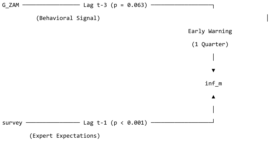
Granger causality tests on the first-differenced series reveal a complementary predictive structure. Survey expectations provide a statistically significant short-term signal for realized inflation at the first lag (p < 0.01). Conversely, the Google search variable (G_ZAM) provides suggestive evidence of a leading behavioral signal at the third lag (p = 0.063). By deploying these features, the framework captures both immediate expert sentiment and early behavioral shifts up to one quarter ahead, as illustrated below.
Figure 2.
Conceptual Predictive Structure of Survey Expectations and Google Search Activity.
3.3.3. Cointegration Analysis
Given the non-stationary nature of the variables, the existence of a long-run equilibrium relationship is examined using the Johansen cointegration test [28]. Establishing cointegration is essential for avoiding spurious regression and confirming that the variables move together over time, notwithstanding short-term fluctuations.
The results summarized in Table 3 show that the trace statistics consistently surpass the 5% critical values across all rank levels. Specifically, the trace statistics of 131.87, 62.70, and 6.41 are above their respective critical values of 29.80, 15.49, and 3.84. These findings suggest a long-run relationship among realized inflation, survey expectations, and Google search activity. Collectively, these results indicate that the variables may share a common long-term trend with an underlying connection that persists despite short-run fluctuations.
3.3.4. Time-Series Decomposition Analysis
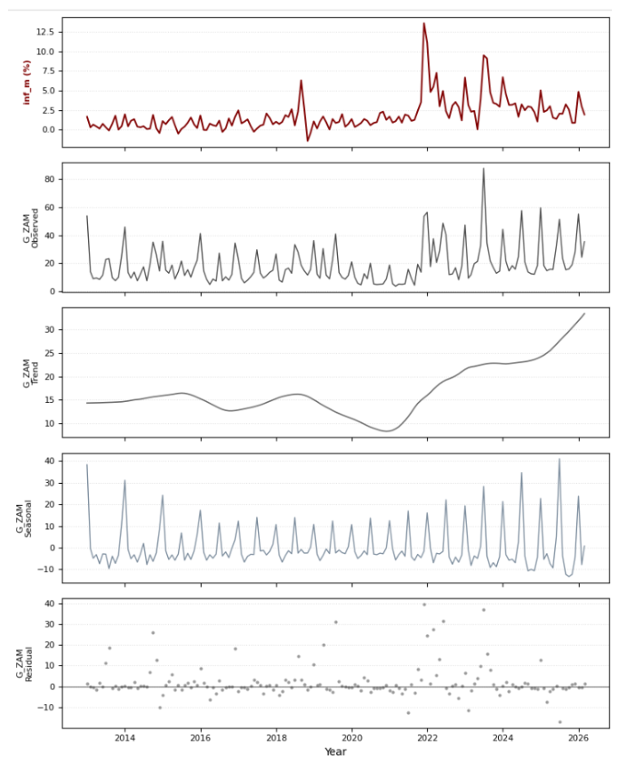
To further explore the structural relationship between inflation and search behavior, both series are decomposed with seasonal-trend decomposition using LOESS (STL) methodology [29]. This procedure separates each series into trend, seasonal, and irregular components.
The decomposition results reveal a pronounced upward trend in both realized inflation and G_ZAM search volumes, particularly after 2021. This pattern is consistent with the structural transformation of Türkiye’s inflation environment, with price pressures becoming more persistent and increasingly salient to consumers.
The seasonal components indicate recurring fluctuations in specific periods; however, these effects remain relatively modest compared to the dominant long-term trend. Consequently, the overall dynamics of both series appear to be driven primarily by structural rather than seasonal factors.
Figure 3.
Time-Series Components of Google Searches.
3.3.5. Structural Break Analysis
The stability of the underlying relationships is assessed using the recursive cumulative sum (CUSUM) test. The resulting test statistic of 8.508 exceeds the 5% critical value of 0.948, indicating significant parameter instability over the sample period. Figure 4 shows that the cumulative sum of recursive residuals crosses the confidence boundaries, confirming the presence of structural breaks and temporal shifts in the data-generating process. These results are consistent with the substantial changes observed in Türkiye’s inflation dynamics during the study period and suggest that standard linear model specifications with static parameters may be insufficient for capturing these evolving structures. The empirical evidence of parameter instability justifies exploring alternative methodologies, such as automated machine learning (AutoML) frameworks, which offer greater flexibility in modeling complex nonlinear structures without imposing rigid structural assumptions.
3.3.6. Endogeneity and Robustness Considerations
Potential endogeneity concerns, including simultaneity and reverse causality between inflation and search activity, are addressed through two primary mechanisms. Explanatory variables are incorporated into the model with lag structures to ensure that information flows from search behavior and expectations to subsequent inflation outcomes. Additionally, the AutoML framework determines optimal lag selection and model architecture in a data-driven manner, thereby reducing specification bias and enhancing robustness.
Within this framework, Google search activity is treated as a quasi-exogenous behavioral signal that precedes official inflation releases. This approach mitigates concerns related to simultaneity, although it does not fully eliminate them.
3.3.7. Summary of Diagnostic Findings
The diagnostic analyses yield several key conclusions:
- All variables satisfy stationarity requirements after transformation and are therefore suitable for time-series modeling.
- Survey-based expectations exhibit strong short-term predictive power for inflation.
- Google search activity demonstrates predictive power over longer horizons and serves as a potential early-warning indicator of inflationary pressures.
- Cointegration results indicate a long-term equilibrium relationship among inflation, expert expectations, and search behavior.
- Time-series decomposition reveals common structural trends, particularly during periods of elevated inflation.
- Structural break tests identify significant regime shifts, supporting the application of adaptive modeling techniques.
Collectively, these findings support the development of a forecasting framework that integrates inflation persistence, expert expectations, and high-frequency behavioral signals within a flexible AutoML environment. The core model specification is therefore expressed as follows:
Here, inf_mt denotes realized monthly inflation, G_ZAMt-3 represents lagged Google search intensity, and surveyt corresponds to inflation expectations obtained from the survey of market participants. The concurrent inclusion of survey expectations at time t is justified by their forward-looking nature. These expectations summarize the most current information set available to market participants and therefore serve as a contemporaneous forecast of inflationary developments, in contrast to the lagged behavioral signals derived from search activity.
3.4. Modeling: AutoML-Based Forecasting Framework
Following data preparation, descriptive analysis, and diagnostic testing, the forecasting stage commences. In time-series applications, model selection is determined by the statistical properties and complexity of the data-generating process. Given the presence of nonlinearity, structural breaks, lagged relationships, and evolving inflation regimes, an AutoML framework is employed to systematically identify optimal forecasting models and automate preprocessing, model selection, and hyperparameter optimization.
The application of AutoML to forecasting problems represents a specialized field referred to as automated time-series analysis. Unlike conventional machine learning approaches, automated time-series frameworks explicitly address temporal dependencies, seasonality, trend components, and lag structures. Libraries such as AutoTS [30] provide an integrated environment in which multiple forecasting architectures are automatically generated, evaluated, and optimized, thereby minimizing subjective model-specification decisions and improving forecasting efficiency [31].
A core component of AutoML is the combined algorithm selection and hyperparameter optimization (CASH) problem, which involves simultaneously identifying the most appropriate algorithm and its optimal parameter configuration. Rather than relying on a single prespecified model, the framework systematically explores a broad search space of competing forecasting methods and evaluates their performance using predefined error metrics. This methodology has received considerable attention in financial econometrics and forecasting research due to its adaptability to complex, nonlinear, and rapidly changing environments [32,33,34,35].
The AutoTS library is chosen for its ability to integrate automated algorithm selection, hyperparameter optimization, and ensemble construction within a unified forecasting environment. The primary objectives are to assess the effectiveness of AutoML techniques in modeling inflation dynamics and determine whether automated forecasting frameworks can surpass conventional econometric approaches in highly volatile environments.
The preliminary analyses presented in the previous section reveal several important characteristics of the dataset. The GSQD series exhibits trend and seasonal patterns, meaningful lag structures identified through causality analysis, and significant structural breaks, particularly after 2021.
Furthermore, the recursive CUSUM test confirms substantial regime shifts in the inflation process. These findings suggest that a single forecasting model may be insufficient to capture all relevant dimensions of the data-generating process. Consequently, a composite modeling strategy is adopted.
Within the AutoTS framework, five complementary forecasting approaches are selected according to empirical performance criteria: autoregressive distributed lag (ARDL), exponential smoothing (ETS), UnivariateMotif, WindowRegression, and ensemble models. Model selection is determined by out-of-sample forecasting performance rather than theoretical considerations. Traditional benchmark models, such as ARIMA and naïve specifications, are evaluated during the optimization process but are ultimately excluded due to inferior forecasting accuracy and higher symmetric mean absolute percentage error (sMAPE) values. Their inability to capture the substantial structural instability observed in the data further supports the adoption of a more adaptive AutoML framework.
Each algorithm offers a distinct analytical capability within the forecasting system. The ARDL model provides a robust econometric structure for capturing lagged effects and long-term relationships among inflation, expectations, and search behavior. ETS models are effective in identifying and extrapolating trend and seasonal patterns using adaptive smoothing mechanisms. WindowRegression applies a flexible regression-based approach that leverages localized temporal relationships within rolling windows. The UnivariateMotif algorithm complements these methods by detecting recurring patterns and nonlinear similarities in historical data, enabling the model to capture dynamics not adequately represented by traditional linear specifications.
To capitalize on the strengths of these individual approaches, the final forecasting architecture utilizes an ensemble framework that integrates predictions from multiple models. Ensemble methods are widely recognized for enhancing forecast robustness by reducing model-specific biases and minimizing the risk of overfitting. This advantage is particularly relevant in inflation forecasting, where volatility, regime changes, and structural uncertainty can compromise the performance of individual models.
Potential endogeneity concerns are addressed by incorporating lagged explanatory variables. Both survey expectations and Google search indicators are included in the forecasting framework with appropriate temporal lags, ensuring that information flows from expectations and behavioral signals to future rather than contemporaneous inflation outcomes. This structure enhances the causal interpretation of predictive relationships and reduces the risk of simultaneity bias.
The AutoML framework adopted in this study offers a flexible, data-driven forecasting environment that accommodates nonlinearities, structural breaks, and evolving economic conditions. By integrating econometric, statistical, pattern-recognition, and ensemble-learning techniques within a unified architecture, the framework seeks to maximize predictive accuracy while maintaining robustness across varying inflation regimes.
Table 4 and Figure 5 provide an overview of the AutoTS workflow and depict the algorithmic architecture used in the empirical analysis.
Within the proposed forecasting framework, the ARDL model provides a robust econometric foundation for capturing both long-run equilibrium relationships and short-term lagged interactions among variables. In contrast, the ETS and WindowRegression models address trend and seasonal dynamics through adaptive smoothing and regression-based mechanisms. The UnivariateMotif algorithm further strengthens the framework by identifying recurring patterns in historical observations, thereby detecting nonlinear structures and temporal similarities that extend beyond conventional linear assumptions.
Integrating these forecasting approaches within an ensemble framework increases predictive robustness and reduces the risk of overfitting that can result from reliance on a single model. This approach is notably important during modeling inflation, which is frequently characterized by structural breaks, regime changes, and periods of heightened volatility.
The forecasting architecture is developed through a systematic, multi-stage workflow:
- Data Integration: Monthly inflation data from the Turkish Statistical Institute (TurkStat), inflation expectations from the TCMB’s survey of market participants, and Google “zam” search data are consolidated into a unified dataset covering the period from 2013 to 2026.
- Data Validation and Cleaning: The dataset is evaluated for completeness and consistency. No missing observations are detected, and correlation analysis shows the absence of severe multicollinearity, as no pairwise correlation exceeds the 0.90 threshold.
- Time-Series Decomposition: STL decomposition is applied to separate trend and seasonal components, improving the signal-to-noise ratio and supporting the extraction of underlying inflation dynamics.
- Feature Engineering: Lagged variables are constructed based on the results of causality analysis. Specifically, a three-period lag of GSQD (t-3) is incorporated to capture persistence effects and the leading-indicator properties of search behavior.
- Automated Optimization: The AutoML engine systematically explores alternative model configurations, feature transformations, and parameter combinations to identify the specification that minimizes the selected forecasting loss function.
- Algorithmic Diversification: Multiple model families are evaluated concurrently to ensure that both linear and nonlinear relationships are represented in the forecasting process.
- Cross-Validation: Model stability and generalization performance are assessed using three-fold time-series cross-validation, which retains the temporal ordering of observations.
- Ensemble Construction: The best-performing individual models are combined through weighted aggregation to generate a hybrid forecast.
- Out-of-Sample Evaluation: Final model performance is evaluated using the last 12 months of previously unseen observations, providing an objective measure of real-world forecasting capability.
Figure 6 presents the optimized model specifications. The AutoML optimization process selects an ARDL-based architecture as the most effective forecasting structure, with an optimal lag configuration of one. These results suggest that short-term persistence and dynamic interactions are the primary factors influencing inflation movements within the proposed framework.
Data preprocessing involves a three-standard-deviation clipping method to manage outliers while preserving data integrity. To isolate behavioral signals from noise, an ElasticNet-based regression filter (L_1 = 0.1) is applied, combined with 90-period rolling trend extraction and an exponentially weighted moving average (EWMA) smoothing filter. This pipeline effectively clarifies the high-frequency signals within the Google search data. Model optimization uses an evolutionary search algorithm to minimize the sMAPE. To maintain temporal validity and prevent look-ahead bias, a threefold backward validation strategy is employed on a 12-month out-of-sample test set. A primary strength of this framework is that the model architecture, lag structures, and hyperparameters are determined endogenously through optimization rather than imposed a priori. This data-driven approach allows the system to adapt to the shifting dynamics of the inflation series, minimizing specification bias. Ultimately, this AutoML environment provides a flexible, robust, and objective forecasting system tailored to the complex nature of inflation.
Forecasting performance is assessed using both the mean absolute percentage error (MAPE) and the sMAPE. The MAPE serves as a standard measure of relative error, whereas the sMAPE is a widely used metric for evaluating predictive accuracy in time-series forecasting. The sMAPE provides a complementary perspective by accounting for symmetric scaling, which is particularly advantageous when analyzing volatile time series. The use of both metrics enables a comprehensive assessment of model accuracy across varying error scales.
The sMAPE measure ranges from 0% to 200%, with lower values indicating superior forecasting performance. In general, values below 10% are considered excellent, values between 10% and 20% indicate high forecasting accuracy, and values above 100% reflect poor predictive capability [36]. It is calculated as follows:
sMAPE = (100% / n) × Σ |Ft − At| / ((|At| + |Ft|) / 2), for t = 1, ..., n
Here, n is the number of observations, At is the observed value, and Ft is the forecasted value.
The proposed forecasting framework achieves an out-of-sample sMAPE of 18.18% over the final 12-month test period, indicating high predictive accuracy and effectively capturing the underlying dynamics of inflation [37].
Figure 7 presents a graphical comparison of realized inflation, survey-based expectations, and forecasts produced by the proposed AutoML framework over the final 12-month out-of-sample period.
Figure 7 demonstrates that the proposed model closely tracks realized inflation throughout the evaluation period. Forecast deviations remain limited, even during episodes of heightened volatility, which suggests that the model effectively captures both the direction and magnitude of inflation movements.
A comparison of the forecast series with market expectations further highlights the value of integrating GSQD into the forecasting framework. Although survey expectations provide a strong baseline predictor, incorporating high-frequency behavioral signals increases the model’s responsiveness to emerging inflationary pressures. As a result, the combined framework generates forecasts that more closely correspond to realized inflation outcomes.
These findings suggest that expert expectations and search-based behavioral indicators provide complementary sources of information. Survey data deliver forward-looking assessments from informed market participants, whereas GSQD reflect real-time shifts in consumer perceptions and responses to price changes. Integrating these sources enhances the model’s capacity to anticipate inflation dynamics, especially during periods of economic uncertainty and rapid adjustment.
In summary, the results demonstrate that combining expert-based expectations with high-frequency behavioral data improves both the timing and accuracy of inflation forecasts. This integration leads to lower prediction errors and a more robust nowcasting framework. Table 5 provides a detailed comparison of forecasted and realized inflation values.
The out-of-sample evaluation indicates that the proposed forecasting framework maintains sound performance during periods of elevated inflation volatility. For example, in January 2026, monthly inflation increased sharply from 0.89% to 4.84%. During this shock episode, the model achieved an absolute error of only 0.22 percentage points, whereas survey-based expectations yielded a substantially larger absolute error of 1.08 percentage points. These results show the model’s capacity to respond rapidly to abrupt changes in inflation dynamics and to outperform traditional expectation-based forecasts during periods of economic turbulence.
More broadly, forecasts based solely on survey expectations yield an average MAPE of 24.62%. Incorporating GSQD into the forecasting framework reduces the average forecasting error to 16.50%. This approximately 32.99% improvement in predictive accuracy provides strong evidence that high-frequency behavioral indicators offer meaningful information beyond what is contained in expert expectations alone.
The statistical robustness of these findings is further supported by Theil’s U-statistic (U2), a widely used measure of relative forecasting performance, particularly in small-sample evaluations [38]. The estimated Theil’s U value of 0.6701 is well below the benchmark value of 1.0, indicating that the proposed model steadily outperforms the survey-based benchmark. This result provides additional evidence of the model’s forecasting efficiency, suggesting that the observed gains reflect genuine improvements in predictive performance rather than random variation.
Collectively, these conclusions indicate that GSQD act not only as supplementary explanatory variables but also as leading indicators that enhance both the responsiveness and precision of inflation forecasts. Their contribution is particularly evident during periods of heightened uncertainty, when traditional survey-based measures may respond more slowly to changing economic conditions.
4. Results and Discussion
To evaluate the real-world forecasting capability of the proposed framework, the final 12 months of observations are reserved as a blind out-of-sample evaluation period. This design provides a more rigorous assessment than in-sample goodness-of-fit measures by testing model performance on previously unseen data.
The empirical findings demonstrate that GSQD can be effectively integrated into inflation nowcasting frameworks and that AutoML-based architectures are capable of capturing both lagged relationships and evolving inflation dynamics. The proposed framework achieves an out-of-sample sMAPE of 18.18%, indicating high predictive accuracy despite substantial macroeconomic volatility and structural change in Türkiye. Moreover, the framework functions as an early-warning mechanism by providing informative signals approximately 10–15 days before the release of official inflation statistics.
To isolate the informational contribution of GSQD, an ablation analysis is performed using alternative model specifications. The results reveal that survey expectations alone generate an average forecasting error of 24.62%, whereas integrating search-based behavioral indicators reduces it to 16.50%, representing an improvement of approximately 32.99%. These findings indicate that GSQD contain substantial predictive information beyond that captured by expert expectations and inflation persistence. Table 6 presents the forecasting performance of the competing model specifications.
The empirical results presented in Table 6 demonstrate the comparative effectiveness of various data channels for forecasting inflation. The baseline error for traditional survey expectations, measured at 24.62%, serves as the primary benchmark for this analysis. The persistence model, which utilizes only historical inflation dynamics, yields a substantially higher error rate of 46.00%. These findings suggest that reliance on past data alone is inadequate for capturing structural breaks in inflation forecasting.
The most notable result and central focus of this study is observed in the model integrating Google search trends, as reflected by GSQD, with survey data. This approach reduces the error rate to 16.50%, representing a substantial relative improvement of 32.98% over the traditional survey benchmark. While the comprehensive model, which incorporates all variables, achieves a performance gain of 17.67%, it does not match the improvement achieved by including search data alone. Collectively, these results underscore the potential of digital behavioral data to address information gaps in traditional expectation surveys and to improve the accuracy of inflation forecasts.
5. Conclusions
This study presents a novel inflation nowcasting framework that combines expert expectations from surveys of market participants with high-frequency behavioral signals from GSQD, implemented within an AutoML environment.
The empirical findings provide varying levels of support for the proposed hypotheses. The first hypothesis receives partial support, as Google search activity exhibits predictive power for future inflation, particularly at longer horizons, although statistical significance is primarily observed at the 10% level rather than the conventional 5% threshold. The second hypothesis is strongly supported: integrating GSQD with survey-based expectations enhances forecasting accuracy by approximately 33% compared to the use of survey expectations alone. The third hypothesis is also supported, with GSQD-based forecasting gains being more substantial during periods of heightened inflation volatility, such as the January 2026 inflation shock. However, this conclusion is based primarily on episode-specific evidence rather than formal regime-switching tests, reflecting a need for future research that employs dedicated volatility frameworks and time-varying parameter models. Notably, the GSQD model reduces the error rate to 16.50% during periods of elevated volatility, when traditional surveys fail to capture sudden price shocks. The findings support H3, confirming that forecasting gains from search data are more pronounced under both high and low inflation volatility. This study advances the literature in four key ways. First, it integrates expert expectations and behavioral search indicators within a unified forecasting framework. Second, it extends inflation nowcasting research by employing an AutoML architecture instead of traditional econometric models. Third, it provides empirical evidence from Türkiye, an emerging economy marked by frequent structural breaks and shifting inflation regimes. Finally, it demonstrates that digital behavioral indicators offer economically meaningful information not fully captured by traditional expectation measures, significantly enhancing forecasting performance.
The findings also have important policy implications. Because Google search activity is available in real time, behavioral indicators can offer early signals of inflationary pressures before the release of official statistics. Such information can guide monetary policy decisions, improve expectation management strategies, and strengthen communication policies during periods of heightened uncertainty. Furthermore, financial institutions may utilize these signals for pricing, portfolio allocation, risk management, and the development of inflation-linked financial products. Therefore, the proposed framework represents both an academic contribution and a practical decision-support tool for institutions operating in rapidly evolving macroeconomic environments.
Several limitations should be acknowledged. First, the analysis relies on a single behavioral keyword (“zam”) as a proxy for inflation perceptions; future research could develop broader search indices that incorporate multiple inflation-related terms. Second, Google Trends provides normalized rather than absolute search volumes, potentially introducing measurement uncertainty. Third, the sample period represents an exceptional macroeconomic environment characterized by high inflation volatility and structural breaks, which may limit the generalizability of the findings to low-inflation economies. Finally, while the AutoML framework effectively captures nonlinear relationships and dynamic changes, its model architecture is less interpretable than that of traditional econometric models.
Future research could strengthen the proposed framework by incorporating additional macro-financial variables, such as exchange rates, energy prices, monetary indicators, and financial conditions. Additionally, employing methodologies specifically designed to capture regime changes, including time-varying parameter models, Markov-switching approaches, and structural-break frameworks, may further enhance forecasting performance and model interpretability.
References
- Thomas, L. B., Jr. Survey measures of expected US inflation. J. Econ. Perspect. 1999, 13(4), 125–144. [Google Scholar] [CrossRef]
- Mehra, Y. P. Survey measures of expected inflation: revisiting the issues of predictive content and rationality. FRB Richmond Econ. Q. 2002, 88(3), 17–36. [Google Scholar]
- Choi, H.; Varian, H. Predicting the present with Google Trends. Econ. Rec. 2012, 88, 2–9. [Google Scholar] [CrossRef]
- Jun, S. P.; Yoo, H. S.; Choi, S. Ten years of research change using Google Trends: From the perspective of big data utilizations and applications. Technol. Forecast. Soc. Change 2018, 130, 69–87. [Google Scholar] [CrossRef]
- Aruoba, S. B.; Diebold, F. X. Real-time macroeconomic monitoring: Real activity, inflation, and interactions. Am. Econ. Rev. 2010, 100(2), 20–24. [Google Scholar] [CrossRef]
- Bok, B.; Caratelli, D.; Giannone, D.; Sbordone, A. M.; Tambalotti, A. Macroeconomic nowcasting and forecasting with big data. Annu. Rev. Econ. 2018, 10(1), 615–643. [Google Scholar] [CrossRef]
- Castle, J. L.; Fawcett, N. W.; Hendry, D. F. Nowcasting is not just contemporaneous forecasting. Natl. Inst. Econ. Rev. 2009, 210, 71–89. [Google Scholar] [CrossRef]
- Costa, E. A.; Silva, M. E. Predicting macroeconomic indicators from online activity data: A review. Stat. J. IAOS 2024, 40(2), 403–419. [Google Scholar] [CrossRef]
- Choi, H.; Varian, H. Predicting the Present with Google Trends; Technical Report; Google Inc, 2009. [Google Scholar] [CrossRef]
- Li, X.; Shang, W.; Wang, S.; Ma, J. A MIDAS modelling framework for Chinese inflation index forecast incorporating Google search data. Electron. Commer. Res. Appl. 2015, 14(2), 112–125. [Google Scholar] [CrossRef]
- Guzman, G. Internet search behavior as an economic forecasting tool: The case of inflation expectations. J. Econ. Soc. Meas. 2011, 36(3), 119–167. [Google Scholar] [CrossRef]
- Suchánek, J. Inflation: Predictive power of Google Trends data. Master’s thesis, Charles University Digital Repository, 2024. Available online: https://dspace.cuni.cz.
- Drachal, K. Forecasting the inflation rate in Poland and US. using dynamic model averaging (DMA) and Google queries. Romanian J. Econ. Forecast. 2020, 23(2), 18–34. [Google Scholar] [CrossRef]
- Wei, Y.; Zhang, X.; Wang, S. Can search data help forecast inflation? Evidence from a 13-country panel. In 2017 IEEE International Conference on Big Data; IEEE, December 2017; pp. 4184–4188. [Google Scholar]
- Bikourne, M.; EL KHAMLICHI, S.; Ez-Zetouni, A.; Akdim, K. Statistical methods for inflation forecasting in Morocco: Insights from Google trends data. Stat. Optim. Inf. Comput. 2025, 13(4), 1636–1653. [Google Scholar] [CrossRef]
- Marcellino, M.; Stevanovic, D. The demand and supply of information about inflation (2022s-27, CIRANO). 2022. [Google Scholar] [CrossRef]
- Jha, S.; Sahu, S. Forecasting inflation for India with the Phillips curve: Evidence from internet search data. Econ. Bull. 2020, 40(3), 2372–2379. [Google Scholar]
- Bicchal, M.; Raja Sethu Durai, S. Rationality of inflation expectations: an interpretation of Google Trends data. Macroecon. Financ. Emerg. Mark. Econ. 2019, 12(3), 229–239. [Google Scholar] [CrossRef]
- Yurevich, M. A. Inflation expectations and inflation: Nowcasting and forecasting. J. Econ. Regul. 2021, 12(2), 22–35. [Google Scholar] [CrossRef]
- Das, P. K.; Das, P. K. Artificial intelligence and inflation forecasting: a contemporary perspective. South Asian J. Macroecon. Public Financ. 2025, 14(1), 133–164. [Google Scholar] [CrossRef]
- Fan, M. H.; Chen, M. Y.; Liao, E. C. A deep learning approach for financial market prediction: Utilization of Google trends and keywords. Granul. Comput. 2021, 6(1), 207–216. [Google Scholar]
- Bolivar, O. High-frequency inflation forecasting: A two-step machine learning methodology. Lat. Am. J. Cent. Bank. 2025, 100172. [Google Scholar]
- Central Bank of the Republic of Türkiye. Survey of market participants. 2026. https://tcmb.gov.tr/wps/wcm/connect/TR/TCMB+TR/Main+Menu/Istatistikler/Egilim+Anketleri/Piyasa+Katilimcilari+Anketi/ (accessed on 30 June 2026).
- ZiraatBank. 2021. https://www.ziraatbank.com.tr/tr/makroekonomik-analizler/turkiye-ekonomisi/temmuz-ayi-tcmb-piyasa-katilimcilari-anketi-enflasyon-ve-buyume-tahminlerinde-yukari-yonlu-revize-surerken-cari-acik-beklentilerinde-azalma-goruluyor (accessed on 30 June 2026).
- D’Acunto, F.; Malmendier, U.; Ospina, J.; Weber, M. Exposure to grocery prices and inflation expectations. J. Political Econ. 2021, 129(5), 1615–1639. [Google Scholar] [CrossRef]
- Eichenauer, V. Z.; Indergand, R.; Martínez, I. Z.; Sax, C. Obtaining consistent time series from Google Trends. Econ. Inq. 2022, 60(2), 694–705. [Google Scholar] [CrossRef]
- Chow, G.C.; Lin, A. Best linear unbiased interpolation, distribution, and extrapolation of time series by related series. Rev. Econ. Stat. 1971, 53(4), 372–375. [Google Scholar] [CrossRef]
- Perron, P.; Campbell, J. Y. A note on Johansen’s cointegration procedure when trends are present. Empir. Econ. 1993, 18(4), 777–789. [Google Scholar] [CrossRef]
- Cleveland, R. B.; Cleveland, W. S.; McRae, J. E.; Terpenning, I. STL: A seasonal-trend decomposition. J. off. Stat. 1990, 6(1), 3–73. [Google Scholar]
- Catlin, C. Adaptive forecasting in dynamic markets: An evaluation of AutoTS within the M6 competition. Int. J. Forecast. 2025. [Google Scholar] [CrossRef]
- Khider, D.; Zhu, F.; Gil, Y. autots: Automated machine learning for time series analysis. In AGU fall meeting abstracts; 2019, December, 2019; Vol. 2019, pp. PP43D–1637. [Google Scholar]
- Gorodetskaya, O.; Gobareva, Y.; Koroteev, M. A machine learning pipeline for forecasting time series in the banking sector. Economies 2021, 9(4), 205. [Google Scholar] [CrossRef]
- Wong, C.; Versace, M. CARTMAP: a neural network method for automated feature selection in financial time series forecasting. Neural Comput. Appl. 2012, 21(5), 969–977. [Google Scholar] [CrossRef]
- Met, I.; Erkoç, A.; Seker, S. E. Performance, efficiency, and target setting for bank branches: time series with automated machine learning. IEEE Access 2022, 11, 1000–1010. [Google Scholar] [CrossRef]
- Met, I.; Erkoc, A.; Seker, S. E.; Erturk, M. A.; Ulug, B. Product recommendation system with machine learning algorithms for SME banking. Int. J. Intell. Syst. 2024, 2024(1), 5585575. [Google Scholar] [CrossRef]
- Jierula, A.; Wang, S.; Oh, T. M.; Wang, P. Study on accuracy metrics for evaluating the predictions of damage locations in deep piles using artificial neural networks with acoustic emission data. Appl. Sci. 2021, 11(5), 2314. [Google Scholar] [CrossRef]
- Chicco, D.; Warrens, M. J.; Jurman, G. The coefficient of determination R-squared is more informative than SMAPE, MAE, MAPE, MSE and RMSE in regression analysis evaluation. PeerJ Comput. Sci. 2021, 7, e623. [Google Scholar] [CrossRef] [PubMed]
- Theil, H.; Scholes, M. Forecast evaluation based on a multiplicative decomposition of mean square errors. Econom. J. Econom. Soc. 1967, 70–88. [Google Scholar] [CrossRef]
Figure 1.
Analytical Workflow.
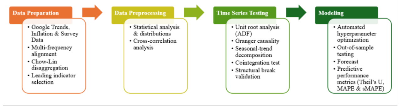
Figure 4.
Recursive CUSUM Plot.
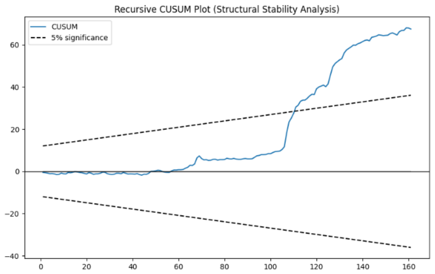
Figure 5.
AutoTS Process Flow.
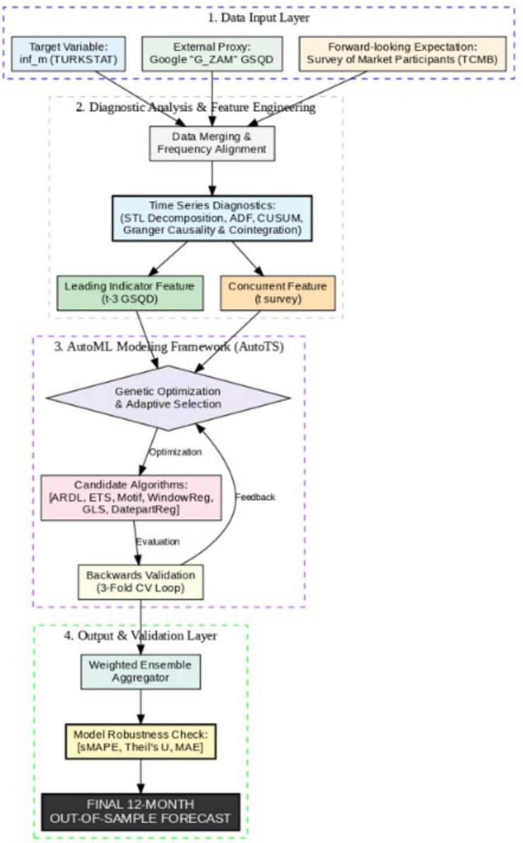
Figure 6.
Best-Performing Model Parameters.
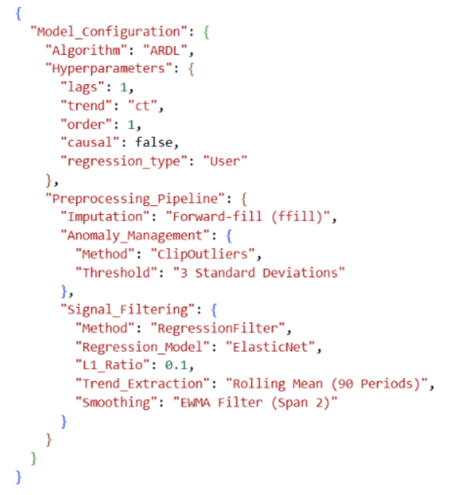
Figure 7.
Comparative Analysis of Realized Inflation, Market Expectations, and Algorithm Forecasts.
Table 1.
Descriptive Statistics of Variables.
| Variable | n | Average | Std. deviation |
Min. | 25% | 50% (median) |
75% | Max. | Skewness | Kurtosis |
|---|---|---|---|---|---|---|---|---|---|---|
| G_ZAM | 162 | 19.17 | 13.54 | 3.70 | 10.00 | 14.98 | 22.66 | 83.21 | 1.78 | 3.79 |
| inf_m | 162 | 1.87 | 2.08 | -1.44 | 0.60 | 1.33 | 2.44 | 13.58 | 2.55 | 9.15 |
| survey | 162 | 1.6 | 1.29 | -0.02 | 0.66 | 1.12 | 2.36 | 6.45 | 1.24 | 1.18 |
Table 3.
Johansen Cointegration Test Results.
| Hypothesized no. of CE(s) | Trace statistic | 5% critical value |
|---|---|---|
| None * | 131.87 | 29.80 |
| 1 * | 62.70 | 15.49 |
| 2 * | 6.41 | 3.84 |
CE: Cointegration equation.
Table 4.
Description of Candidate Forecasting Models.
| Selected algorithms | Description |
|---|---|
| Ensemble | A hybrid algorithm in which the best-performing individual models are combined through optimal weighting to minimize forecast errors |
| ARDL | An algorithm that analyzes both short- and long-run cointegration relationships between dependent and independent variables, as well as their lagged effects |
| ETS | An algorithm that applies exponential smoothing by decomposing the time series into error, trend, and seasonality components |
| UnivariateMotif | An algorithm that identifies historical patterns and recurring cyclical movements (motifs) in the dataset and performs pattern matching for future forecasting |
| WindowRegression | An algorithm that performs local regression on the series through rolling time windows, ensuring swift adaptation to dynamic shifts |
| Generalized least squares (GLS) | An algorithm that estimates linear regression parameters while explicitly accounting for autocorrelation and heteroscedasticity within the residuals, which are common in macroeconomic time series |
| DatepartRegression | A regression-based algorithm that automatically extracts and utilizes temporal features (e.g., month, quarter) from the datetime index to capture complex calendar effects and deterministic seasonality |
Table 5.
Comparison of Model Results.
| Date | Real inflation (inf_m) | Model prediction | Survey expectation | Absolute error (model) | Absolute error (survey) |
|---|---|---|---|---|---|
| 2025-07 | 2.06 | 2.34 | 2.11 | 0.28 | 0.05 |
| 2025-08 | 2.04 | 1.64 | 1.69 | 0.40 | 0.35 |
| 2025-09 | 3.23 | 2.19 | 2.04 | 1.04 | 1.19 |
| 2025-10 | 2.55 | 2.26 | 2.34 | 0.29 | 0.21 |
| 2025-11 | 0.87 | 0.95 | 1.59 | 0.08 | 0.72 |
| 2025-12 | 0.89 | 0.84 | 1.08 | 0.05 | 0.19 |
| 2026-01 | 4.84 | 4.62 | 3.76 | 0.22 | 1.08 |
| 2026-02 | 2.96 | 2.35 | 2.54 | 0.61 | 0.42 |
| 2026-03 | 1.94 | 2.11 | 2.18 | 0.17 | 0.24 |
| 2026-04 | 4.18 | 3.05 | 2.93 | 1.13 | 1.25 |
| 2026-05 | 1.71 | 1.14 | 1.89 | 0.57 | 0.18 |
| 2026-06 | 0.99 | 1.11 | 1.36 | 0.12 | 0.37 |
Table 6.
Forecasting Performance of the Models.
| Model specification | Variables included | MAPE | Relative improvement |
|---|---|---|---|
| Benchmark survey model | Survey expectations | 24.62% | - |
| Persistence model | Lagged inflation (t-1) | 46.0% | -86.84% |
| Survey + inflation persistence | Survey + lagged inflation (t-1) | 19.53% | 20.67% |
| *Survey + GSQD (best model) | Survey + GSQD (t-3) | 16.50% | 32.99% |
| Comprehensive model | Survey + GSQD (t-3) + lagged inflation (t-1) | 20.27% | 17.67% |
Disclaimer/Publisher’s Note: The statements, opinions and data contained in all publications are solely those of the individual author(s) and contributor(s) and not of MDPI and/or the editor(s). MDPI and/or the editor(s) disclaim responsibility for any injury to people or property resulting from any ideas, methods, instructions or products referred to in the content. |
© 2026 by the authors. Licensee MDPI, Basel, Switzerland. This article is an open access article distributed under the terms and conditions of the Creative Commons Attribution (CC BY) license (http://creativecommons.org/licenses/by/4.0/).
Copyright: This open access article is published under a Creative Commons CC BY 4.0 license, which permit the free download, distribution, and reuse, provided that the author and preprint are cited in any reuse.


