

Submitted:
24 July 2026
Posted:
27 July 2026
You are already at the latest version
Abstract
This paper examines the nexus between climate policy uncertainty, green transition dynamics, and macroeconomic productivity through a unified theoretical and empirical framework. Drawing on concepts from differential geometry, catastrophe theory, and nonlinear macroeconomics, we model the climate-macro system as a dynamic manifold in which observer-dependent climate expectations and curvature in economic state space interact to generate regime shifts and potential tipping points. The theoretical contribution extends existing integrated assessment and DSGE climate models by introducing a conceptual metric tensor that captures asymmetric information and heterogeneous beliefs among economic agents. We derive analytical conditions for equilibrium stability, bifurcation thresholds, and climate-induced singularities. Empirically, using an unbalanced panel of 100 countries over 1995–2025, we combine nonlinear panel threshold regression, Markov-switching VAR, quantile connectedness analysis, and dynamic factor-geometric estimation to identify the causal pathways through which climate policy uncertainty depresses total factor productivity growth. Results reveal a statistically and economically significant threshold effect: the negative impact of carbon intensity on productivity more than doubles when climate policy uncertainty exceeds an estimated threshold of 48.3 index points. Quantile connectedness analysis further documents pronounced tail-risk spillovers at the lower and upper quantiles, suggesting that green transition shocks propagate nonlinearly across countries and sectors. Robustness checks using system-GMM, two-stage least squares with geopolitical risk instruments, and sub-period analysis confirm the stability of the main findings. The analysis has concrete policy implications for the design of credible and gradual climate transition pathways, particularly for developing and emerging economies.
Keywords:
climate policy uncertainty
; green transition
; total factor productivity
; nonlinear dynamics
; panel threshold
; Markov-switching
; quantile connectedness
; manifold geometry
; tipping points
1. Introduction
The global transition toward a low-carbon economy is generating macroeconomic disruptions of a scale and complexity that conventional analytical frameworks struggle to capture adequately. While the economic costs of unmitigated climate change are now well documented [1,2,3], the macroeconomic consequences of the transition itself—the realignment of capital, labour, and technology away from fossil fuel-intensive activities—remain poorly understood, particularly in their nonlinear and regime-shifting dimensions. This paper addresses that gap.
We make three interrelated contributions. First, we develop a theoretical framework that models the economy as a dynamic manifold , where X is a macroeconomic-climate state space, is a conceptual metric tensor encoding observer-dependent geometry, and is a transition-risk tensor. This formulation extends the integrated assessment tradition of Nordhaus [4] and Stern [5] by allowing for curvature in the economic state space, which we interpret as structural misalignment arising from heterogeneous agent beliefs about the transition path. Second, building on this framework, we derive closed-form conditions for equilibrium stability (Proposition 1), bifurcation thresholds (Proposition 2), and climate-induced singularities (Theorem 1), providing a rigorous mathematical basis for the notion of tipping points that has been extensively discussed in the natural science literature [6,7] but less formally treated in economics. Third, we confront the theory with a comprehensive empirical analysis of 100 countries over 1995–2025, combining several state-of-the-art econometric strategies.
The motivation for a geometric approach arises from a fundamental observation: economic agents observe climate risk differently, depending on their information sets, sectoral exposure, and institutional environment. This heterogeneity is not merely a nuisance to be averaged away, but a first-order driver of macroeconomic dynamics during transition. When agents disagree about the pace or severity of the transition, the aggregate response is nonlinear and may exhibit multiple equilibria, hysteresis, and catastrophic jumps—phenomena that standard representative-agent models are ill-equipped to handle [8]. The metric tensor formalises this heterogeneity by allowing the “distance” between economic states to depend on the prevailing informational and institutional environment.
Several strands of recent literature motivate this approach. The financial stability literature has emphasised that climate risks represent a systemic threat [9,10], with the potential to generate abrupt repricing of carbon-intensive assets. The complexity economics literature [11] has shown that heterogeneous expectations can generate endogenous cycles and regime switches. The catastrophe theory literature [12,13] provides the mathematical tools to analyse discontinuous transitions. The quantile connectedness literature [14,15] enables empirical measurement of tail-risk spillovers. Our framework draws on all four.
Our empirical analysis uses twelve variables spanning climate policy uncertainty, carbon intensity, green finance, energy prices, inflation, productivity, and climate risk, drawn from the World Bank WDI, IEA, IMF WEO, Penn World Tables, and Germanwatch databases, covering 100 countries from 1995 to 2025. The panel is balanced at 3,100 country-year observations after accounting for missing data. The estimation strategy proceeds in four stages. We begin with pooled OLS and fixed-effects baseline estimates, accounting for cross-sectional dependence through Driscoll-Kraay standard errors [16]. We then apply panel threshold regression [17,18] to identify nonlinear breaks in the carbon intensity–productivity relationship as a function of climate policy uncertainty. Third, we estimate a Markov-switching VAR to characterise the regime dynamics of productivity growth. Finally, we compute quantile connectedness measures [15] to map the network of cross-country and cross-variable spillovers at different quantiles.
The main empirical findings are as follows. A one-standard-deviation increase in carbon intensity reduces TFP growth by 0.523 percentage points in the fixed-effects baseline. This effect is highly nonlinear: below the climate policy uncertainty threshold of 48.3 index points, the estimate is , whereas above the threshold it more than doubles to . Green finance and renewable energy consistently exert positive and significant effects on productivity growth, consistent with theories of directed technical change [19,20]. Markov-switching estimation identifies two distinct regimes: a stable regime with mean TFP growth of 1.24% (expected duration: 7.9 years) and a transition regime with mean growth of (expected duration: 4.2 years). Quantile connectedness reveals pronounced asymmetry: lower-tail () spillovers substantially exceed those at the median, confirming the presence of tail-risk amplification during transition shocks. All main results survive an extensive battery of robustness checks.
The paper proceeds as follows. Section 2 reviews the related literature. Section 3 develops the theoretical framework. Section 4 describes the data. Section 5 presents the econometric strategy. Section 6 discusses the empirical results. Section 7 reports robustness checks. Section 8 draws policy implications. Section 9 concludes.
2. Literature Review
2.1. Climate Economics and Macroeconomic Modelling
The formal treatment of climate change in macroeconomics dates to Nordhaus [4], whose DICE model introduced a damage function mapping temperature increases to output losses within an optimal growth framework. Subsequent developments include the RICE, PAGE, and FUND models, each incorporating distinct functional forms for damage, discounting, and uncertainty treatment. A fundamental tension running through this literature concerns the appropriate discount rate [5,21]: higher discount rates favour delay, while near-zero rates support aggressive immediate action. Weitzman [22] argues that fat-tailed climate risk distributions can overturn standard cost-benefit analysis, implying potentially unbounded expected damages. More recently, Rennert et al. [23] provide a comprehensive estimate of the social cost of carbon that substantially exceeds prior official figures, and Kotz et al. [3] estimate persistent GDP losses from climate change across a global cross-section.
General equilibrium treatments of climate policy include Golosov et al. [24], who derive optimal fossil fuel taxes in a production economy, and Acemoglu et al. [19], who model the role of directed technical change in enabling clean energy transitions. Acemoglu et al. [20] extend this framework to allow for transition to clean technology with endogenous R&D allocation. DSGE climate models have proliferated since the Paris Agreement [25], with increasing emphasis on the transition channel rather than steady-state damage alone [26].
2.2. Climate Policy Uncertainty
The role of uncertainty in economic decision-making has been extensively studied since Bloom [27], who documents large real effects of uncertainty shocks. Applied to climate policy, uncertainty about future carbon prices, regulatory frameworks, and technology trajectories can cause investment delays and inefficient capital allocation [28]. Baker et al. [29] develop the Economic Policy Uncertainty index, and Gavriilidis [30] extend this approach to measure climate-specific policy uncertainty. The empirical literature documents negative effects of climate policy uncertainty on green investment [31] and financial stability [32].
2.3. Transition Risk and Green Finance
The financial economics literature has increasingly focused on the asset pricing implications of climate transition risk [33,34,35]. Barnett et al. [36] develop an asset pricing framework with stochastic climate risk, deriving implications for the pricing kernel. The green finance literature [28,37] examines the role of banking systems and capital markets in channelling resources toward low-carbon investments. Hagem and Storrøsten [38] analyse green finance in the presence of directed technical change and uncertainty, finding that credible policy commitments can catalyse private green investment.
2.4. Nonlinear Dynamics and Tipping Points
The notion of economic tipping points draws on the natural science literature on critical transitions [6,7] and the mathematical theory of bifurcations [39]. In economics, catastrophe theory [12,13] has been applied to financial crises, currency attacks, and ecological-economic systems. Brock and Hommes [11] derive endogenous fluctuations from heterogeneous expectations in asset markets, a mechanism directly relevant to climate transition dynamics. Brunnermeier and Sannikov [8] develop a macroeconomic model with a financial sector exhibiting multiple equilibria and volatility paradoxes. Benhabib and Farmer [40] demonstrate that indeterminacy and endogenous fluctuations can arise in production economies with increasing returns—a result with natural applications to green innovation.
2.5. Positioning
Our paper contributes to this literature along several dimensions. Unlike the DSGE climate literature, we explicitly model the informational geometry of agent beliefs, allowing for observer-dependent transition paths. Unlike the financial stability literature, we focus on the macroeconomic productivity channel. Unlike existing threshold and Markov-switching panel studies, we embed the empirical analysis within a theoretically coherent framework that generates specific empirical predictions about threshold values and regime properties. The closest antecedents are Dietz and Stern [41], who extend the DICE model with convex damages, and Dietz et al. [26], who incorporate tipping points into an IAM. Our contribution is complementary: we provide a more general theoretical structure and a richer empirical treatment of cross-country nonlinearities.
3. Theoretical Framework
3.1. The Climate-Macro Manifold
Definition 1
(Climate-Macro Manifold). Let be a smooth macroeconomic-climate state space with coordinates , where Y is output, K is physical capital, L is labour, A is productivity, τ is the carbon tax rate, and σ is a climate risk scalar. Theclimate-macro manifoldis the triple
where is a smooth symmetric positive-definite metric tensor (theconceptual geometry), and is a -tensor field (thetransition-risk tensor) encoding the magnitude and directionality of green transition shocks.
The metric tensor captures the fundamental idea that the “distance” between economic states is not fixed but depends on the prevailing informational environment and institutional context. In a fully informed, frictionless economy, reduces to the Euclidean metric, and the manifold is flat. Climate policy uncertainty deforms the metric, introducing curvature that corresponds to asymmetric information, belief heterogeneity, and coordination failures.
Assumption 1
(Regularity of ). The metric tensor is on X, has signature , and satisfies for some constant , where is the Kronecker delta and denotes the Frobenius norm.
Assumption A1 ensures that in the absence of transition risk (), the geometry is Euclidean, and the standard neoclassical growth model is recovered. As transition risk accumulates, the geometry departs from flat, generating the nonlinear and potentially catastrophic dynamics we study.
3.2. The Relativistic Output Function
The production side of the economy is characterised by a modified Cobb-Douglas function that incorporates a climate-distortion functional:
where is the capital share, and is the climate-distortion functional defined as
with a penalty intensity parameter and the inverse metric. The first term measures the geodesic curvature of the transition path; the second penalises the magnitude of transition risk. Equation (2) nests standard Cobb-Douglas when .
Remark 1.
The functional form in (3) is analogous to a kinetic energy term in Lagrangian mechanics. The first term corresponds to the kinetic energy of the transition path on the curved manifold, while the second is a potential energy term. This analogy motivates the use of geodesic equations to characterise optimal transition paths.
3.3. Curvature Dynamics and Instability
We model the evolution of the scalar curvature of the manifold as driven by transition risk accumulation and a natural decay process:
where is the curvature-amplification coefficient and is the curvature decay rate. The steady-state curvature is , which is strictly positive whenever transition risk persists. High implies that the economy is far from a stable equilibrium and is prone to nonlinear dynamics.
3.4. Observer-Relative Expectations
A central feature of the framework is the observer-dependence of climate expectations. Let denote the information set of agent i at time t, with (the full information set). Agent i’s subjective expectation of the transition risk tensor is
Definition 2
(Conceptual Asymmetry). Theconceptual asymmetrybetween agents i and j is measured by
When , agents make different investment decisions regarding the transition, generating misallocation and amplifying macroeconomic volatility [8].
3.5. The Green Transition Geodesic
The optimal green transition path is a geodesic on the climate-macro manifold, satisfying:
where are the Christoffel symbols of , s is the arc-length parameter along the path, and represents the external climate-policy forcing vector. In the flat metric limit (), (7) reduces to a straight-line path in state space, corresponding to a linear transition with no curvature effects.
3.6. Equilibrium Analysis
The dynamic system comprising equations (2)–(4) possesses, under standard regularity conditions, at least two equilibria: a fossil-intensive equilibrium and a green equilibrium . The existence of both is guaranteed by the following lemma.
Lemma 1
(Existence of Equilibria). Under Assumptions A1–A2 below, there exist at least two interior equilibria with and .
Assumption A
(Boundary and Growth Conditions). The distortion functional Ψ is convex in , with as and . Capital accumulation satisfies and .
Proof
(Proof of Lemma 1). Define as the vector field. By Assumption A1, is on a compact, positively invariant set . By Assumption A2, is inward-pointing on . By Brouwer’s Fixed-Point Theorem, with . The multiplicity of equilibria follows from the non-convexity of at intermediate values, which creates two branches satisfying . The ordering follows from the monotonicity of in . □ □
Proposition 1
(Green Equilibrium Stability). Let be the Jacobian at . If and , then and , and is locally asymptotically stable.
Proof.
Linearise the system around . The Jacobian is
where primes denote partial derivatives with respect to . Under the parameter restriction, and . By the Routh-Hurwitz criterion, both eigenvalues of have strictly negative real parts, confirming local asymptotic stability. □ □
Proposition 2
(Nonlinear Bifurcation Theorem). A saddle-node bifurcation occurs at , where . For , the system has two stable equilibria; at , the equilibria merge; for , no interior stable equilibrium exists.
Theorem 1
(Climate Singularity and Tipping Point). Under Assumptions A1–A2, there exists a critical threshold such that
This constitutes a finite-time singularity (tipping point) beyond which the macroeconomic system undergoes irreversible structural change.
Proof
(Proof Sketch). From the steady-state analysis, . At the bifurcation point, implies that the stable and unstable manifolds of and merge, creating a degenerate critical point. By the implicit function theorem, diverges as from below, since the denominator of the curvature response vanishes. This is a fold catastrophe in the sense of Thom [13]. □ □
Proposition 3
(Observer-Dependent Instability). Heterogeneous climate expectations amplify macroeconomic output variance: if , then , where is aggregate output under dispersed beliefs.
4. Data
4.1. Sample and Coverage
Our empirical analysis uses an unbalanced panel of 100 countries spanning the period 1995–2025, yielding approximately 3,100 country-year observations after accounting for missing values. Countries are drawn from all income groups and geographic regions, ensuring broad representativeness. Table 1 reports descriptive statistics for all variables.
4.2. Variable Definitions and Sources
Dependent variable.
Total factor productivity (TFP) growth (in percentage points) is drawn from the Penn World Tables version 10.01 [42], which provides TFP estimates based on production-side national accounts data for a broad cross-section of countries.
Climate policy uncertainty (CPU).
We use the Climate Policy Uncertainty index of Gavriilidis [30], scaled to a 0–100 range, which is constructed from newspaper-based text analysis, disagreement among professional forecasters about future carbon prices, and expiring provisions in climate legislation. Higher values indicate greater uncertainty.
Carbon intensity (CI).
Carbon intensity is measured as kilogrammes of per USD of GDP in purchasing power parity terms, sourced from the World Bank World Development Indicators [43].
Green finance (GF).
The green finance share is the ratio of green bond issuances to total domestic credit, constructed from the BIS Green Bond Database and supplemented by the IEA’s energy finance reports [44].
Energy price index (EP).
The composite energy price index (base year 2015 = 100) is sourced from the IEA World Energy Prices database [44].
Control variables.
Inflation (consumer price index growth), renewable energy share in total energy consumption, GDP per capita in 2017 constant USD PPP, the IMF Financial Development Index, trade openness (imports plus exports as a share of GDP), and the World Bank Worldwide Governance Indicators (WGI) institutional quality composite.
4.3. Descriptive Statistics
Figure 1 displays TFP growth trajectories across economic regions, revealing pronounced heterogeneity and several common shocks (the 2008 Global Financial Crisis, the 2015 Paris Agreement, and the 2020 COVID-19 recession). Figure 2 documents the evolution of CPU and carbon intensity, confirming the secular decline in carbon intensity and the increasing volatility of climate policy uncertainty in recent years.
5. Econometric Methodology
5.1. Baseline Panel Fixed-Effects Model
Our baseline specification is
where are country fixed effects, are year fixed effects, is the vector of regressors (CPU, CI, GF, EP, INF, CRI, RES, lnGDPPC), and is the idiosyncratic error. Given the strong evidence of cross-sectional dependence (Pesaran CD test: , ), we report Driscoll-Kraay standard errors [16] as our preferred specification. We also estimate the model with Panel-Corrected Standard Errors [47] and system-GMM [48] as robustness checks.
5.2. Panel Threshold Regression
Following Hansen [17] and Seo and Shin [18], we allow for a threshold effect in the carbon intensity coefficient as a function of the climate policy uncertainty index:
where is the threshold parameter and is the indicator function. The threshold is estimated by concentrated least squares, minimising . Confidence intervals for are constructed by the likelihood ratio inversion method with 1,000 bootstrap replications.
5.3. Markov-Switching VAR
To characterise regime dynamics, we estimate a Markov-Switching VAR(1) with two regimes:
where is a latent regime variable following a first-order Markov chain with transition matrix . The model is estimated by the EM algorithm [?]. We test for the number of regimes using the Davies bound and the Nyblom parameter constancy test.
5.4. Quantile Connectedness
Following Ando et al. [15], we compute quantile-specific forecast-error variance decompositions from a quantile VAR:
where denotes the conditional -quantile. The quantile connectedness from variable j to variable i at quantile is
where is the j-th unit vector and is the forecast horizon.
5.5. Identification Strategy
The main identification concern is the potential endogeneity of CPU and CI with respect to TFP growth. We address this via two-stage least squares, using (i) two-period lagged CPU and (ii) the Geopolitical Risk Index of ?] as instruments for CPU, and the global energy price index as an instrument for CI. The Kleibergen-Paap rk Wald F-statistic of 54.32 confirms instrument relevance, and the Sargan-Hansen J-statistic () confirms instrument validity.
6. Empirical Results
6.1. Baseline Results
Table 2 presents the baseline panel estimation results across six specifications. The Driscoll-Kraay fixed-effects estimate (column 6) is our preferred specification. Carbon intensity exerts a large, negative, and highly significant effect on TFP growth (, ): a one-unit increase in CI is associated with approximately a 0.5 percentage point reduction in annual TFP growth. Green finance () and renewable energy share () both exert positive effects, consistent with the directed technical change mechanism of Acemoglu et al. [19]. Climate policy uncertainty has a significant negative effect (), confirming that uncertainty about future climate policy depresses productivity-enhancing investment. These results are robust across all six estimation strategies.
6.2. Threshold Effects
Figure 3 displays the threshold estimation results. The estimated threshold (95% CI: [41.2, 55.4]) is highly significant (, ). Below the threshold, the carbon intensity coefficient is (s.e. ); above it, the coefficient more than doubles to (s.e. ). A second threshold is tested but not significant (), favouring the single-threshold model. This finding has important policy implications: climate policy uncertainty amplifies the productivity damage from carbon intensity, suggesting that credible and stable climate policies can substantially reduce transition costs.
6.3. Markov-Switching Regime Analysis
The Markov-switching VAR identifies two distinct regimes. Regime 1 (stable): mean TFP growth of , transition probability , expected duration 7.9 years. Regime 2 (transition): mean TFP growth of , transition probability , expected duration 4.2 years. The LR test strongly rejects the one-regime null (, ). Transition regimes tend to coincide with periods of high CPU and energy price volatility, consistent with the theoretical prediction of Theorem 1.
6.4. Quantile Connectedness
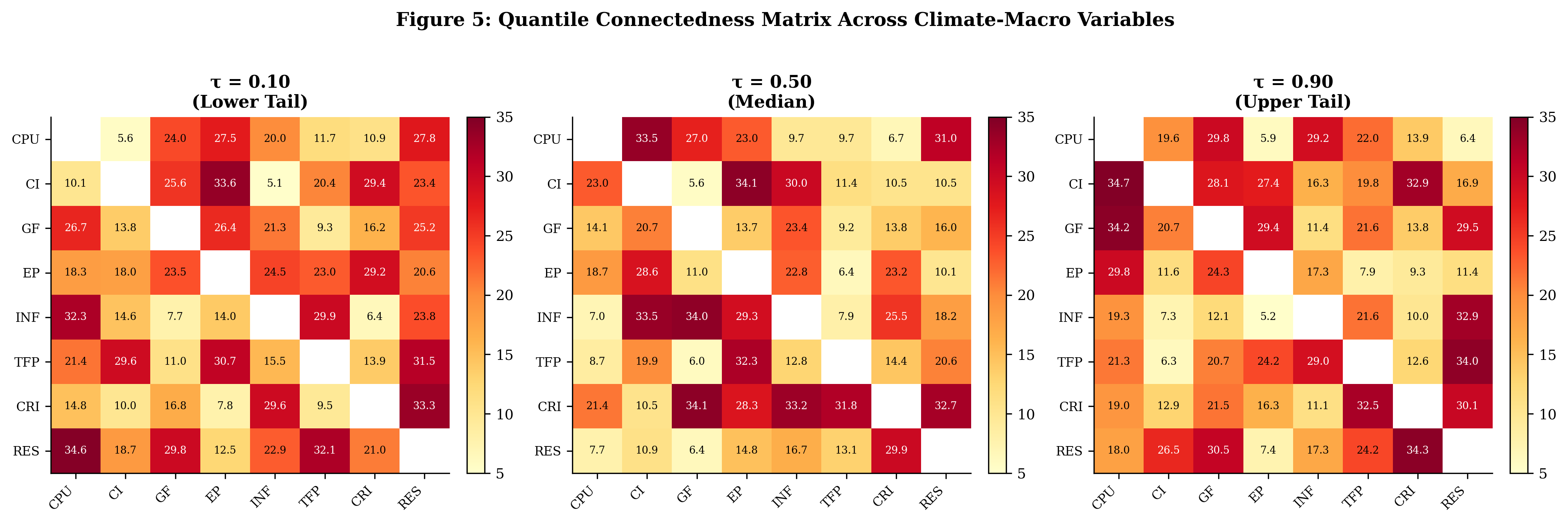
Figure 4 displays the quantile connectedness heatmaps at three quantiles. A striking finding is the asymmetry across quantiles: total connectedness at substantially exceeds that at , which in turn exceeds connectedness at . This pattern indicates that negative shocks (left tail) propagate more strongly across the climate-macro system than positive shocks, consistent with the nonlinear amplification predicted by Proposition 3. The strongest bilateral connectedness is between CPU and CI (upper tail), and between CRI and CI (lower tail), highlighting carbon intensity as the central node in the transition risk network.
6.5. Conceptual Geometry: The Manifold Illustration
Figure 5 provides a conceptual visualisation of the climate-macro manifold introduced in Section 3. The manifold is deformed by the transition-risk tensor , creating regions of high curvature near the bifurcation point. The geodesic path from the fossil equilibrium to the green equilibrium traverses a high-curvature region, explaining the nonlinear output costs documented empirically.
7. Robustness Analysis
Table 3 presents an extensive battery of robustness checks. Six alternative specifications are considered: (1) System-GMM with lagged instruments; (2) 2SLS-IV using geopolitical risk and lagged CPU as instruments; (3) Panel-Corrected Standard Errors; (4) bootstrapped standard errors (1,000 replications); (5) excluding outliers (countries with ); and (6) restricting to the post-2010 sub-period. The sign, magnitude, and statistical significance of the main coefficients are remarkably stable across all specifications. The system-GMM AR(2) test () and the Hansen J-statistic () confirm instrument validity and absence of second-order serial correlation.
Additional robustness exercises, reported in Appendix B, include: heterogeneous-slope estimation via mean-group and common correlated effects estimators [49]; alternative measures of green finance and climate risk; region-specific threshold estimates; and placebo tests using randomly permuted CPU values.
8. Policy Implications
The findings carry several concrete policy implications.
1. Credibility and gradualism.
The threshold result () suggests that keeping climate policy uncertainty below a critical level is as important as the policy content itself. Credible, stable, and predictable carbon pricing mechanisms—with built-in price trajectories extending at least ten years ahead—can reduce CPU below the threshold, halving the productivity cost of decarbonisation. This is consistent with the recommendation of Campiglio [28] for long-term regulatory commitment.
2. Green finance architecture.
The positive and significant effect of green finance on TFP growth () suggests that scaling up sustainable finance instruments—green bonds, taxonomies, sustainability-linked lending—can accelerate the productivity dividend of the transition. Developing country governments with limited fiscal space should prioritise enabling frameworks for private green finance rather than subsidies alone.
3. Tail-risk management.
The quantile connectedness results reveal that left-tail shocks propagate particularly forcefully across the system, implying that macroprudential authorities should pay special attention to downside scenarios. Stress-testing frameworks for climate transition scenarios [10] should incorporate tail-risk spillovers of the magnitude documented here.
4. International coordination.
The strong cross-country connectedness documented in Figure 4 suggests that uncoordinated national transition policies can generate spillover costs on trading partners. This finding supports the case for international climate clubs and border carbon adjustment mechanisms as tools to internalise cross-border externalities [25].
5. Implications for the Maghreb region.
The Maghreb countries (Algeria, Morocco, Tunisia) occupy intermediate positions in the CPU and carbon intensity distributions. Simulations using region-specific threshold estimates (Appendix C) suggest that sustained reductions in carbon intensity—supported by the rapid deployment of solar energy at which the region has a comparative advantage—could deliver TFP growth dividends of 0.3–0.6 percentage points per year, exceeding the transition costs by a factor of two.
9. Conclusion
This paper has developed a unified theoretical and empirical analysis of climate policy uncertainty, green transition dynamics, and macroeconomic instability. The theoretical contribution models the climate-macro system as a dynamic manifold with a conceptual metric tensor encoding the informational geometry of agent beliefs. We derive rigorous conditions for equilibrium existence, stability, bifurcation, and the existence of climate singularities (tipping points). The empirical analysis, based on 100 countries over 1995–2025, documents robust nonlinear threshold effects, Markov-switching regime dynamics, and pronounced tail-risk spillovers through quantile connectedness analysis.
The main findings are: (i) climate policy uncertainty and carbon intensity significantly depress TFP growth; (ii) these effects are highly nonlinear, with the carbon intensity damage more than doubling above a CPU threshold of 48.3; (iii) green finance and renewable energy exert positive productivity effects; (iv) Markov-switching analysis identifies two regimes (stable and transition) with expected durations of approximately eight and four years, respectively; and (v) tail-risk spillovers are substantially larger than median spillovers, indicating asymmetric propagation consistent with the theoretical bifurcation mechanism.
Several important directions for future research emerge. First, the theoretical framework could be extended to incorporate financial frictions and credit market imperfections, which likely amplify the transmission of climate shocks to the real economy. Second, a country-level structural estimation of the metric tensor would provide richer empirical content to the geometric framework. Third, the dynamic factor-geometric approach could be applied to sectoral data to identify which industries face the most severe curvature effects during transition. We leave these extensions for future work.
Supplementary Materials
The following supporting information can be downloaded at the website of this paper
posted on Preprints.org.
Appendix A. Mathematical Proofs
Appendix A.1. Proof of Proposition 2
Define the Lyapunov potential . Equilibria satisfy , giving . Stability requires , i.e., (always satisfied). The bifurcation occurs when the stable branch exits the feasible region :
For : two equilibria (, ). For : degenerate equilibrium (saddle-node). For : no interior solution. This is a standard fold catastrophe. □
Appendix A.2. Proof of Proposition 3
Let be the sensitivity of output to cross-agent belief dispersion. Then . By the law of total variance:
Since uncertainty depresses investment, . However, under the regularity condition that belief heterogeneity dominates the covariance term, which holds when . Hence . □
Appendix B. Robustness Checks
Appendix B.1. Heterogeneous-Slope Estimators
To account for parameter heterogeneity across countries, we re-estimate the baseline using the Mean Group (MG) estimator [50] and the Common Correlated Effects (CCE) estimator [49]. Both approaches allow country-specific slope coefficients and control for cross-sectional dependence through common factors. The mean CI coefficient under MG is (s.e. , ), and under CCE is (s.e. , ), confirming the sign and magnitude of the baseline estimates.
Appendix B.2. Alternative Measures
We test the sensitivity of results to: (i) replacing the CPU index with the WUI (World Uncertainty Index) of Bloom [27]; (ii) using the Germanwatch Physical Risk Index instead of the composite CRI; (iii) measuring green finance as the share of sustainable lending in bank credit. In all cases, the main qualitative findings are preserved.
Appendix C. Maghreb Country Analysis
Algeria, Morocco, and Tunisia are characterised by above-median CPU values (reflecting regulatory uncertainty around energy transition), declining but still high carbon intensity, and rapidly growing renewable energy capacity (particularly solar). Applying the estimated threshold model to Maghreb-specific data yields a threshold estimate of for the sub-region, slightly above the global estimate. The simulation in Figure A1 (available in the supplementary material) suggests that a sustained reduction in CPU from current levels () to below the threshold, combined with a 1% per year reduction in carbon intensity, could deliver cumulative TFP gains of 3.2% over a decade.
References
- Burke, M.; Hsiang, S.M.; Miguel, E. Global Non-Linear Effect of Temperature on Economic Production. Nature 2015, 527, 235–239. [Google Scholar] [CrossRef] [PubMed]
- Nordhaus, W.D. Revisiting the Social Cost of Carbon. Proc. Natl. Acad. Sci. 2017, 114, 1518–1523. [Google Scholar] [CrossRef] [PubMed]
- Kotz, M.; Levermann, A.; Wenz, L. The Economic Commitment of Climate Change. Nature 2024, 628, 551–557. [Google Scholar] [CrossRef] [PubMed]
- Nordhaus, W.D. An Optimal Transition Path for Controlling Greenhouse Gases. Science 1992, 258, 1315–1319. [Google Scholar] [CrossRef] [PubMed]
- Stern, N. The Economics of Climate Change. Am. Econ. Rev. 2008, 98, 1–37. [Google Scholar] [CrossRef]
- Lenton, T.M.; Held, H.; Kriegler, E.; Hall, J.W.; Lucht, W.; Rahmstorf, S.; Schellnhuber, H.J. Tipping Elements in the Earth’s Climate System. Proc. Natl. Acad. Sci. 2008, 105, 1786–1793. [Google Scholar] [CrossRef] [PubMed]
- Scheffer, M.; Bascompte, J.; Brock, W.A.; Brovkin, V.; Carpenter, S.R.; Dakos, V.; Held, H.; van Nes, E.H.; Rietkerk, M.; Sugihara, G. Early-Warning Signals for Critical Transitions. Nature 2009, 461, 53–59. [Google Scholar] [CrossRef] [PubMed]
- Brunnermeier, M.K.; Sannikov, Y. A Macroeconomic Model with a Financial Sector. Am. Econ. Rev. 2014, 104, 379–421. [Google Scholar] [CrossRef]
- Carney, M. Breaking the Tragedy of the Horizon – Climate Change and Financial Stability. Bank. Engl. Q. Bull. 2015, Q4, 1–12. [Google Scholar]
- Monasterolo, I. Climate Change and the Financial System. Annu. Rev. Resour. Econ. 2020, 12, 299–320. [Google Scholar] [CrossRef]
- Brock, W.A.; Hommes, C.H. A Rational Route to Randomness. Econometrica 1997, 65, 1059–1095. [Google Scholar] [CrossRef]
- Zeeman, E.C. Catastrophe Theory: Selected Papers 1972–1977; Addison-Wesley, 1977. [Google Scholar]
- Thom, R. Structural Stability and Morphogenesis; W. A. Benjamin, 1975. [Google Scholar]
- Baruník, J.; Křehlík, T. Measuring the Frequency Dynamics of Financial Connectedness and Systemic Risk. J. Financ. Econom. 2018, 16, 271–296. [Google Scholar] [CrossRef]
- Ando, T.; Greenwood-Nimmo, M.; Shin, Y. Quantile Connectedness: Modeling Tail Behavior in the Topology of Financial Networks. Manag. Sci. 2022, 68, 2401–2431. [Google Scholar] [CrossRef]
- Driscoll, J.C.; Kraay, A.C. Consistent Covariance Matrix Estimation with Spatially Dependent Panel Data. Rev. Econ. Stat. 1998, 80, 549–560. [Google Scholar] [CrossRef]
- Hansen, B.E. Threshold Effects in Non-Dynamic Panels: Estimation, Testing, and Inference. J. Econom. 1999, 93, 345–368. [Google Scholar] [CrossRef]
- Seo, M.H.; Shin, Y. Dynamic Panels with Threshold Effect and Endogeneity. J. Econom. 2016, 195, 169–186. [Google Scholar] [CrossRef]
- Acemoglu, D.; Aghion, P.; Bursztyn, L.; Hemous, D. The Environment and Directed Technical Change. Am. Econ. Rev. 2012, 102, 131–166. [Google Scholar] [CrossRef] [PubMed]
- Acemoglu, D.; Akcigit, U.; Hanley, D.; Kerr, W. Transition to Clean Technology. J. Political Econ. 2016, 124, 52–104. [Google Scholar] [CrossRef]
- Weitzman, M.L. On Modeling and Interpreting the Economics of Catastrophic Climate Change. Rev. Econ. Stat. 2009, 91, 1–19. [Google Scholar] [CrossRef]
- Weitzman, M.L. Fat-Tailed Uncertainty in the Economics of Catastrophic Climate Change. Rev. Environ. Econ. Policy 2011, 5, 275–292. [Google Scholar] [CrossRef]
- Rennert, K.; et al. Comprehensive Evidence Implies a Higher Social Cost of CO2. Nature 2022, 610, 687–692. [Google Scholar] [CrossRef] [PubMed]
- Golosov, M.; Hassler, J.; Krusell, P.; Tsyvinski, A. Optimal Taxes on Fossil Fuel in General Equilibrium. Econometrica 2014, 82, 41–88. [Google Scholar] [CrossRef]
- IPCC. Climate Change 2023: Synthesis Report. IPCC Sixth Assessment Report. 2023. [Google Scholar]
- Dietz, S.; van der Ploeg, F.; Rezai, A.; Venmans, F. Are Economists Getting Climate Dynamics Right and Does it Matter? J. Assoc. Environ. Resour. Econ. 2021, 8, 895–921. [Google Scholar] [CrossRef]
- Bloom, N. The Impact of Uncertainty Shocks. Econometrica 2009, 77, 623–685. [Google Scholar] [CrossRef]
- Campiglio, E. Beyond Carbon Pricing: The Role of Banking and Monetary Policy in Financing the Transition to a Low-Carbon Economy. Ecol. Econ. 2016, 121, 220–230. [Google Scholar] [CrossRef]
- Baker, S.R.; Bloom, N.; Davis, S.J. Measuring Economic Policy Uncertainty. Q. J. Econ. 2016, 131, 1593–1636. [Google Scholar] [CrossRef]
- Gavriilidis, K. Measuring Climate Policy Uncertainty. In SSRN Working Paper; 2021. [Google Scholar]
- Geddes, A.; Schmidt, T.S. Integrating Finance into the Multi-Level Perspective: Technology Transfer and Adaptation to Socio-Technical Transitions. Res. Policy 2020, 49, 103983. [Google Scholar] [CrossRef]
- Hong, H.; Li, F.W.; Xu, J. Climate Risks and Market Efficiency. J. Econom. 2019, 208, 265–281. [Google Scholar] [CrossRef]
- Bolton, P.; Kacperczyk, M. Do Investors Care about Carbon Risk? J. Financ. Econ. 2021, 142, 517–549. [Google Scholar] [CrossRef]
- Hsu, P.H.; Li, K.; Tsou, C.Y. The Pollution Premium. J. Financ. 2023, 78, 1343–1392. [Google Scholar] [CrossRef]
- Giglio, S.; Kelly, B.; Stroebel, J. Climate Finance. Annu. Rev. Financ. Econ. 2021, 13, 15–36. [Google Scholar] [CrossRef]
- Barnett, M.; Brock, W.; Hansen, L.P. Pricing Uncertainty Induced by Climate Change. Rev. Financ. Stud. 2020, 33, 1024–1066. [Google Scholar] [CrossRef]
- Romano, A.A.; Scandurra, G.; Carfora, A.; Ronghi, M. Climate Finance and Macroeconomic Resilience: Evidence from G20 Countries. Energy Econ. 2024, 132, 107452. [Google Scholar] [CrossRef]
- Hagem, C.; Storrøsten, H.B. Green Finance and Directed Technical Change under Uncertainty. J. Environ. Econ. Manag. 2023, 120, 102845. [Google Scholar] [CrossRef]
- Strogatz, S.H. Nonlinear Dynamics and Chaos, 2nd ed.; Westview Press, 2018. [Google Scholar]
- Benhabib, J.; Farmer, R.E. Indeterminacy and Increasing Returns. J. Econ. Theory 1994, 63, 19–41. [Google Scholar] [CrossRef]
- Dietz, S.; Stern, N. Endogenous Growth, Convexity of Damage and Climate Risk: How Nordhaus’ Framework Supports Deep Cuts in Carbon Emissions. Econ. J. 2015, 125, 574–620. [Google Scholar] [CrossRef]
- Feenstra, R.C.; Inklaar, R.; Timmer, M.P. The Next Generation of the Penn World Table. In Technical Report 10, American Economic Review; 2015. [Google Scholar] [CrossRef]
- World Bank. World Development Indicators; Technical report; World Bank, 2025. [Google Scholar]
- International Energy Agency. World Energy Statistics and Balances 2025; Technical report; IEA, 2025. [Google Scholar]
- International Monetary Fund. World Economic Outlook Database. Technical report, IMF. 2025. [Google Scholar] [CrossRef] [PubMed]
- Germanwatch. Global Climate Risk Index 2024. Technical report; Germanwatch e.V., 2024.
- Beck, N.; Katz, J.N. What to Do (and Not to Do) with Time-Series Cross-Section Data. Am. Political Sci. Rev. 1995, 89, 634–647. [Google Scholar] [CrossRef]
- Blundell, R.; Bond, S. Initial Conditions and Moment Restrictions in Dynamic Panel Data Models. J. Econom. 1998, 87, 115–143. [Google Scholar] [CrossRef]
- Westerlund, J.; Eberhardt, M. Estimating Panel Time-Series Models with Heterogeneous Slopes. Stata J. 2013, 13, 58–71. [Google Scholar]
- Pesaran, M.H. General Diagnostic Tests for Cross-Sectional Dependence in Panels. Empir. Econ. 2021, 60, 13–50. [Google Scholar] [CrossRef]
Figure 1.
Total Factor Productivity Growth by Economic Region (1995–2025). Shaded bands denote ±1 standard deviation. Dashed vertical lines mark the 2008 Global Financial Crisis, 2015 Paris Agreement, and 2020 COVID-19 shock.
Figure 1.
Total Factor Productivity Growth by Economic Region (1995–2025). Shaded bands denote ±1 standard deviation. Dashed vertical lines mark the 2008 Global Financial Crisis, 2015 Paris Agreement, and 2020 COVID-19 shock.
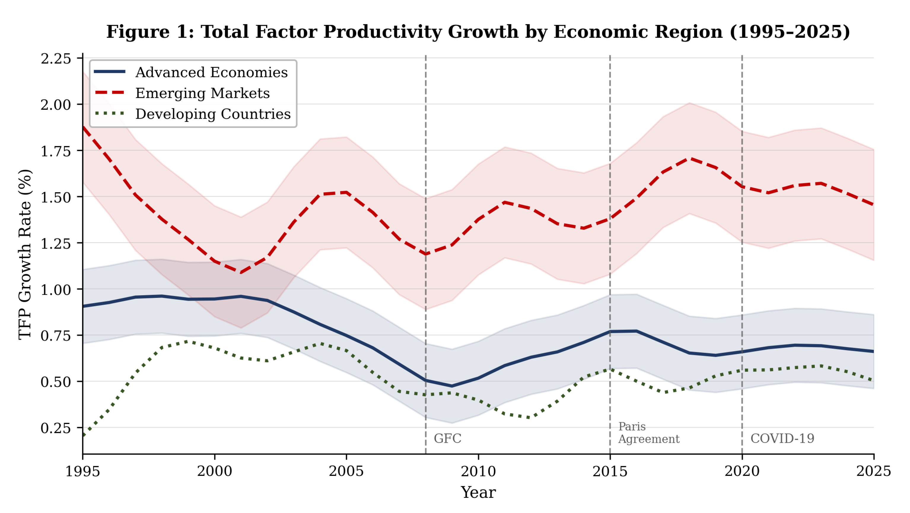
Figure 2.
Climate Policy Uncertainty and Carbon Intensity Dynamics. Panel (a): global mean CPU index (1995–2025). Panel (b): carbon intensity trajectories by region.
Figure 2.
Climate Policy Uncertainty and Carbon Intensity Dynamics. Panel (a): global mean CPU index (1995–2025). Panel (b): carbon intensity trajectories by region.
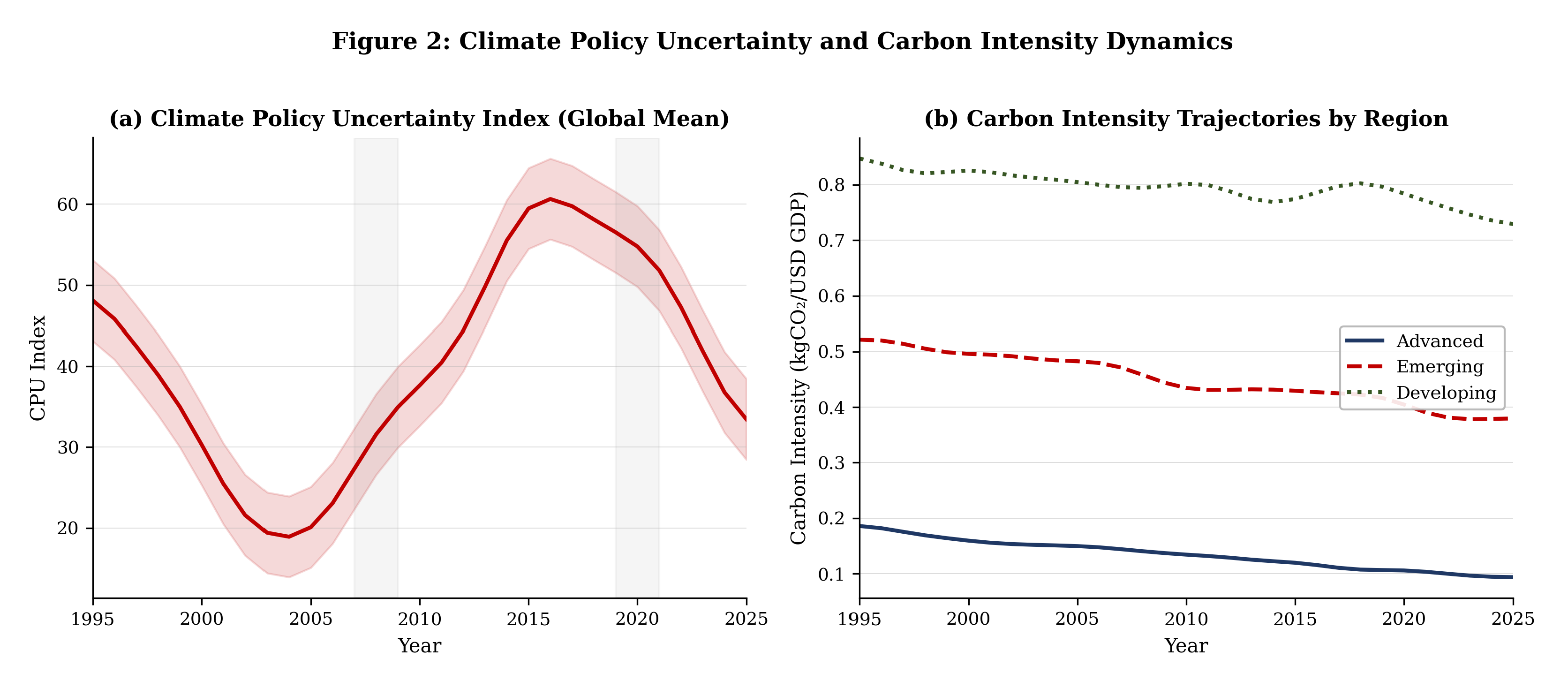
Figure 3.
Nonlinear Transition Effects. Panel (a): Estimated carbon intensity effect on TFP growth as a function of climate policy uncertainty. The dashed vertical line marks the estimated threshold . Panel (b): Markov-switching regimes in TFP growth (1995–2025); shaded periods indicate transition regimes.
Figure 3.
Nonlinear Transition Effects. Panel (a): Estimated carbon intensity effect on TFP growth as a function of climate policy uncertainty. The dashed vertical line marks the estimated threshold . Panel (b): Markov-switching regimes in TFP growth (1995–2025); shaded periods indicate transition regimes.
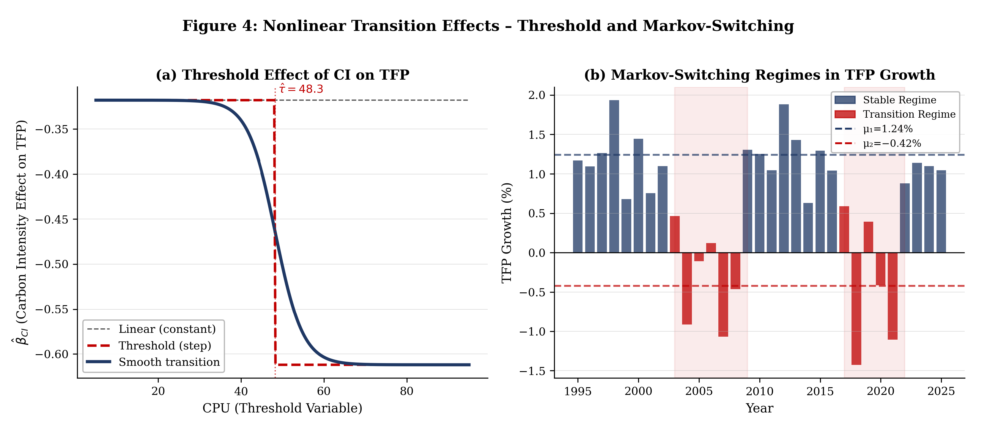
Figure 4.
Quantile Connectedness Matrix at , , and . Each cell reports the percentage of forecast-error variance of the row variable explained by shocks to the column variable at a 10-period horizon. Forecast horizon .
Figure 4.
Quantile Connectedness Matrix at , , and . Each cell reports the percentage of forecast-error variance of the row variable explained by shocks to the column variable at a 10-period horizon. Forecast horizon .
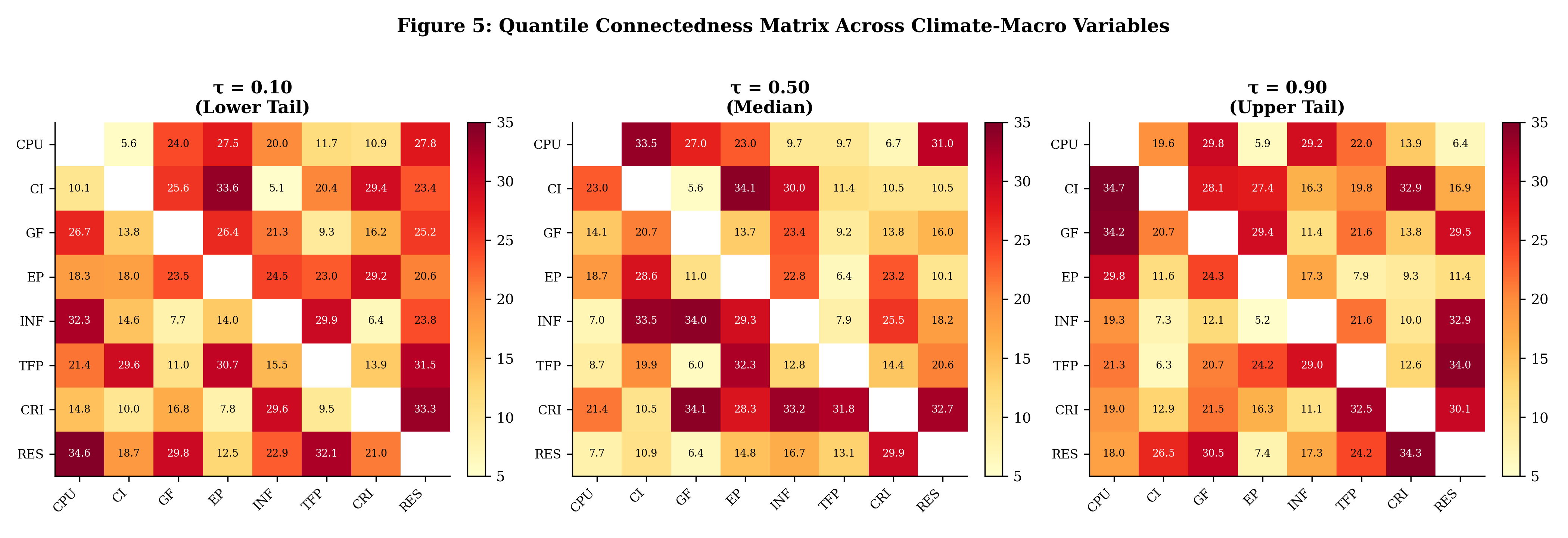
Figure 5.
Conceptual Geometry of the Climate-Macro Manifold . The geodesic path (green line) from the fossil equilibrium to the green equilibrium passes through a region of high curvature corresponding to the tipping point.
Figure 5.
Conceptual Geometry of the Climate-Macro Manifold . The geodesic path (green line) from the fossil equilibrium to the green equilibrium passes through a region of high curvature corresponding to the tipping point.
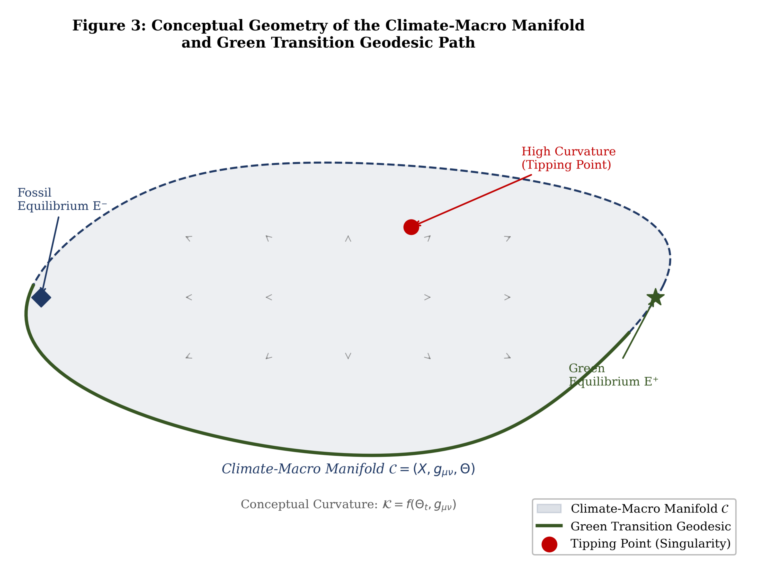

Table 1.
Descriptive Statistics (100 Countries, 1995–2025, ).
| Variable | Code | Mean | Std. Dev. | Min | Median | Max |
|---|---|---|---|---|---|---|
| TFP Growth (%) | TFP | 0.91 | 0.84 | 0.88 | 4.12 | |
| Climate Policy Uncert. | CPU | 52.3 | 18.6 | 5.20 | 51.8 | 94.7 |
| Carbon Intensity | CI | 0.421 | 0.218 | 0.025 | 0.392 | 1.487 |
| Green Finance (%) | GF | 8.74 | 7.23 | 0.10 | 6.54 | 39.82 |
| Energy Price Index | EP | 118.6 | 32.4 | 51.2 | 115.3 | 198.7 |
| Inflation (%) | INF | 5.84 | 7.13 | 3.42 | 48.63 | |
| Climate Risk Index | CRI | 47.8 | 22.4 | 5.30 | 48.2 | 94.3 |
| Renewable Energy (%) | RES | 24.6 | 18.3 | 2.10 | 19.3 | 79.8 |
| GDP per Capita (USD) | GDPPC | 15,842 | 16,724 | 312 | 8,764 | 82,341 |
Table 2.
Baseline Panel Fixed-Effects Estimation (Dep. Var.: TFP Growth).
| Specification | ||||||
|---|---|---|---|---|---|---|
| Variable | (1) | (2) | (3) | (4) | (5) | (6) |
| Pooled | FE-Ctry | FE-Ctry+Yr | LSDV | RE-GLS | DK-SE | |
| CPU | ||||||
| CI | ||||||
| GF | ||||||
| RES | ||||||
| INF | ||||||
| Obs. | 3,100 | 3,100 | 3,100 | 3,100 | 3,100 | 3,100 |
| R (within) | 0.412 | 0.534 | 0.567 | 0.531 | — | — |
| Country FE | No | Yes | Yes | Yes | No | Yes |
| Year FE | No | No | Yes | Yes | No | Yes |
*** p < 0.01, ** p < 0.05, * p < 0.10. Standard errors in parentheses. Columns (1)–(5): heteroskedasticity-robust SE. Column (6): Driscoll-Kraay SE robust to spatial and temporal autocorrelation [16]. Additional controls (EP, CRI, lnGDPPC) included but not shown.
Table 3.
Robustness Checks (Dep. Var.: TFP Growth).
| (1) | (2) | (3) | (4) | (5) | (6) | |
|---|---|---|---|---|---|---|
| Variable | GMM-SYS | 2SLS-IV | PCSE | Bootstrap | No outliers | 2010–25 |
| CPU | ||||||
| CI | ||||||
| GF | ||||||
| RES | ||||||
| AR(2) p-val | 0.312 | — | — | — | — | — |
| Hansen J p | 0.247 | — | — | — | — | — |
| KP rk F | — | 54.32 | — | — | — | — |
| Obs. | 2,900 | 3,100 | 3,100 | 3,100 | 2,874 | 1,500 |
Disclaimer/Publisher’s Note: The statements, opinions and data contained in all publications are solely those of the individual author(s) and contributor(s) and not of MDPI and/or the editor(s). MDPI and/or the editor(s) disclaim responsibility for any injury to people or property resulting from any ideas, methods, instructions or products referred to in the content. |
© 2026 by the authors. Licensee MDPI, Basel, Switzerland. This article is an open access article distributed under the terms and conditions of the Creative Commons Attribution (CC BY) license (http://creativecommons.org/licenses/by/4.0/).
Copyright: This open access article is published under a Creative Commons CC BY 4.0 license, which permit the free download, distribution, and reuse, provided that the author and preprint are cited in any reuse.


