
Submitted:
16 July 2026
Posted:
22 July 2026
You are already at the latest version
Abstract
Return on Equity (ROE) is one of the most closely monitored financial ratios by shareholders
and potential investors. A negative ROE can send an unfavourable message to
investors. This study identifies the financial ratios that influence ROE and determines
the best machine learning technique for predicting it. The imbalanced dataset, sourced
from the Integrated Real-time Equity System (IRESS), consisted of all companies listed
on the Johannesburg Stock Exchange in 2019. The dataset was balanced using original
observations from previous years (dataset 2) and the SMOTE and ROSE oversampling
methods. Additionally, we assessed the performance of three shrinkage methods— Lasso,
Elastic Net, and Ridge Regression—specifically for feature selection. The model evaluation
metrics used are sensitivity, specificity, precision, F1 score, and accuracy. The best predictors
of ROE identified by the classifiers were net profit margin, interest cover, earnings per
share, earnings yield, and price-to-earnings ratio. The Random Forest method emerged
as the most effective feature selection technique. With the SMOTE and ROSE datasets,
performance decreased after feature selection. After oversampling, it was not easy to
choose between the SMOTE and ROSE datasets because RF performed very well on both,
with key metrics above 99%. The study encourages investors to prioritize companies with
low price-to-earnings ratios, high net profit margins, high interest cover, high earnings
per share, and high earnings yield when making investment decisions, using the Random
Forest method.
Keywords:
classification
; k-nearest neighbour
; logistic regression
; machine learning
; naive bayes
; random forest
; return on equity
; stock exchange
; shrinkage methods
; ROSE
; SMOTE
1. Introduction
Every investor needs accurate information before investing in the capital market. Incorrect information can mislead investors in making sound investment decisions and result in losses for them [28,29]. The Stock Exchange provides fair and transparent pricing for listed companies to limit the risk of share trading and has strict regulations that all listed companies must comply with [23]. The largest stock exchange in Africa is the Johannesburg Stock Exchange (JSE), also known as the Johannesburg Securities Exchange [9]. The main aim of every investor is to maximize profit and minimize loss; hence, comparing different companies using the right tools is very important before investing.The best way to compare different companies in the financial market is through financial ratios [4]. It is also the most popular and widely used financial analysis tool [5,16]. Profitability ratios, the most widely used financial ratios, are primarily used to determine whether a company will succeed or fail. Return on Equity (ROE) is a financial ratio used by investors to check whether their investments are profitable (Josue, 2015) [18]. From an investor’s perspective, a higher ROE indicates a higher rate of return on investment [31]. ROE is calculated as
ROE is used to check if the company is heading in the right direction financially, however ROE must be used with other ratios to be reliable [22]. The primary objective of this study is to find determinants of ROE, using a binary dependent variable ROE.
1.1. Motivation and Objectives
Many studies have been conducted in the past to identify financial ratios that influence ROE, but all use a continuous dependent variable. Various methods, such as the DuPont formula, Correlation analysis, and multiple linear regression (MLR), have been used to identify determinants of ROE. However, all those methods are limited in one way or another. Both the DuPont formula and correlation analysis are limited in that they cannot be used to find a collective influence of ROE, nor can they be used to predict ROE. The limitation of MLR is its stringent assumptions, which are often not met, leading to biased and inconsistent results [19]. According to [10], negative ROE communicates a loss to shareholders. [27] stated that a positive ROE indicates shareholders are gaining, while a negative ROE indicates shareholders are incurring losses on their investment. Since ROE can be either positive or negative, using continuous dependent variable neglects the negative part of ROE or loss of information, when negative ROE is converted into positive ROE. Hence we chose binary dependent variable which combines both positive and negative ROE. For binary purposes, ROE was coded as follows
The primary objective of this study is to fit a logistic regression (LR), random forest (RF), k-nearest neighbour (KNN), and naive bayes (NB) to the data using the binary dependent variable ROE, to find the determinants of ROE, while the secondary objective is to identify the best machine learning (ML) technique that can predict ROE. The limitation of the model is that, no value will be produced by the model but can only predict whether ROE will be positive or negative.
This study will help investors identify companies likely to deliver better returns on their investments. Investment managers will also benefit from this research, since with ratios that influence ROE at their disposal they will be able to come up with strategy to enhance ROE of their company. It will also provide answers as to which machine learning technique can be used to predict ROE for companies listed on the Johannesburg Stock Exchange and other Stock Exchanges.
1.2. Literature Review
Many researchers have studied financial ratios in the capital market that may yield dividends to an investor. Also, there have been many studies on identifying the best Machine learning (ML) to adopt across many fields of endeavour.
1.2.1. Return on Equity
[24] investigated the impact of total asset turnover and DTE ratio on ROE for listed companies on the Indonesian Stock Exchange. The companies selected were from the automotive industry, and their components were sampled with a sample size of 50. Ten companies were selected. The statistical technique used to analyze the data was multiple linear regression. They concluded that the Debt-to-Equity ratio negatively affects ROE, while Total Asset Turnover positively affects ROE. It was also found that DTE and Total Asset Turnover combined do affect ROE.
[5] conducted a study to examine the influence of the Quick ratio (QR), DTE ratio, and Total Asset Turnover on ROE for companies listed on the Indonesia Stock Exchange for the period 2012 to 2019. The test of the classical assumption was conducted in SPSS version 25. The relationship between ROE and the Quick ratio was found to be positive but insignificant. ROE and Total Asset Turnover also showed a positive, but insignificant, relationship. It was the Debt-to-Equity ratio that had a negative but insignificant relationship. The three independent variables, taken together, showed a negative association with ROE, but the effect was not significant.
[12] conducted a study to examine the impact of capital structure and financial characteristics on profitability among Jordanian service-sector companies listed on the Amman Stock Exchange. The independent variables used were capital structure, consisting of Debt to Equity (DTE) and Debt to Assets (DTA). The financial characteristics consisted of business risk, growth, size, and tangible assets. Their findings were that size and growth positively impact profitability, namely, EBIT-TA and ROE.
Kim21 used Oaxaca decomposition and regression analysis to examine the diversity of financial performance among listed food product manufacturers in Vietnam for the period 2014 to 2019. The independent variables used were Quick ratios, total assets turnover ratios, leverage ratios, company size, sales growth, and CPI. They concluded that growth in sales and total assets turnover does impact ROE and Return on sales. It was also discovered that leverage ratios negatively impact Return on sales.
[34] used panel data regression analysis to identify financial indicators that statistically influence ROA and ROE in the energy sector in Turkey. The companies targeted were gas, oil, electricity, and renewable energy producers and distributors in Turkey that are listed on the Borsa Istanbul Stock Exchange. The period targeted was 2010, Quarter 1, to 2019, Quarter 4. The two dependent variables used were ROE and ROA. The predictors were firm size, receivable turnover ratio, interest cover ratio, receivable turnover in days, price-to-book, current ratio, asset turnover ratio, leverage ratio, quick ratio, price-to-earnings, inventory turnover ratio, cost of sales ratio and EBIT margin. Sixteen companies were identified, and the sample size was 640 observations. The variables found to influence ROE were quick ratio, leverage ratio, receivable turnover ratio, inventory turnover ratio, firm size, and cost of sales ratio. In contrast, ROA was influenced by the receivables turnover ratio, cost of sales ratio, quick ratio, and price-to-book ratio.
[36] breaks down ROA into Net Profit Margin and Assets Turnover. To find determinants of ROE, they used ROA, Net Profit Margin, and Total Assets as independent variables. The listed companies on the Thai Stock Exchange for the period 2015 to 2019 were used to collect secondary data, with two sample sizes of 104 and 93. The combination of Total Assets and Net Profit Margin outperformed ROA in predicting ROE.
All the research above used a continuous dependent variable, ROE. Most of them were analyzed using Multiple Linear Regression (MLR), which requires many model assumptions to yield valid and reliable results. These assumptions are often not met; hence, in this study, we seek to use a binary dependent variable for ROE.
1.2.2. Machine Learning Methods
Tutcu24 used ML methods to determine whether the firms of IT sector listed at Borsa Istanbul Stock Exchange are profitable. They used financial data sourced from technology sector which consisted of 13 firms listed for the period 2000 to 2023. The two dependent variables that were estimated were ROE and ROA using ML methods in the form of Decision tree (DT), Multiple Linear Regression (MLR) and Artificial Neural Networks (ANN). It was found that the ML methods that were effective in predicting ROE and ROA were ANN and MLR.
[17] constructed models to predict ROA and ROE using retail companies located in Vietnamese. The ML methods used were Multilayer Perceptron XGBoost and Random Forest. The data was collected from financial statements of listed retail companies and the period used were from 2010 to 2024. The best predicting model was found to be RF with RMSE of 0.0926 followed by XGboost.
[37] implemented seven ML techniques — Decision Tree (DT), LR, Support Vector Machine (SVM), Neural Networks, KNN, NB, and RF — to predict heart disease. The research used health care data from the University of California, Irvine ML repository, with a sample size of 303:139 were positive and 164 were negative. The highest classification accuracy was achieved by Artificial Neural Networks (92.30%), while RF, LR, KNN, and NB achieved 85.71%, 81.71%, 80.21%, and 57.14%, respectively.
To detect fraud in financial accounting for Turkish Small and Medium Enterprises (SME) from different sectors, [14] compared ML techniques in the form of NB, KNN, LR, Support Vector Machine, Artificial Neural Network, RF and Bagging. The data was collected from one of the leading credit provider bank in Turkey and the number of firms used was 341 Turkish SME for the period 2013 to 2017. The sample size used was a highly unbalanced dataset of 1705, consisting of 321 fraudulent cases and 1384 non-fraudulent cases. Their finding was Random Forest outperformed the rest with an accuracy of 93.74%, meanwhile KNN, LR and NB had an accuracy of 89.92%, 88.08% and 58.81% respectively.
[6] used Google Colab to compare LR, KNN, SVM, RF, DT, and NB for breast cancer classification. The dataset was obtained from Wisconsin public records and comprises 569 cases (212 benign and 357 malignant). The number of features used, sourced from biopsy images, was ten (10), consisting of symmetry fractal, concave points, compactness, area, texture, radius, perimeter, smoothness, concavity, and dimension. The top classifier was logistic regression, with an accuracy of 98.5%. Meanwhile, KNN, RF, and NB had classification accuracies of 96.97%, 94.99%, and 93.47%, respectively.
To compare ML techniques in the classification of breast cancer, [3] used thirteen machine learning techniques, which are Bayes Net K2 search, Bayes Net Tab search, Lazy-KStar, Bayes TAN search, NB, LR, Lazy-IBK, Rules Zero R, Trees Decision stump, Lazy LWY, Trees J48, RF, and Trees Random trees. The dataset was analyzed using Waikato Environment for Knowledge Analysis (WEKA) software with a sample size of 699 and 10 independent variables. Lazy-IBK and K Nearest Neighbor achieved the highest classification with an accuracy of 98.2%, while RF, NB, LR, and NB achieved 96.4%, 96.4%, and 92.8%, respectively.
In breast cancer classification, [6] found that LR outperformed other ML techniques, while [3] found that Random Forest outperformed them. This suggests that more research using different datasets is needed. It is also unclear which ML method is best for classification. In this research, we aim to extend the comparison of the four ML models to the Stock Exchange Market.
2. Materials and Methods
2.1. The Dataset, Research Variables and missing values
The data was sourced from the Integrated Real-time Equity System (IRESS) website. IRESS contains a database of financial ratios for companies listed on the JSE from 1970. The dataset was collected using simple random sampling, selecting all companies listed on the JSE for the year 2019. We did not display Company names to protect the privacy of each company. The number of predictors before checking for multicollinearity among predictors was ten (10). One predictor was removed due to multicollinearity. The sample comprised 323 companies: 236 with positive ROE and 87 with negative ROE. To address the issue of the imbalanced dataset, the following methods were used:
- Firstly, the 2019 original imbalance dataset (dataset 1) was analysed using metrics such as precision, recall, ROC-AUC score, and F1 score, which are known to cope with imbalanced datasets. We also included accuracy to see how it would be affected by the imbalanced dataset.
- Secondly, the 2019 dataset was balanced using observations from previous years (dataset 2) while ensuring independence of observations. The observations to balance the dataset were selected from companies listed between 2000 and 2018. For each selected company, we selected one observation without missing values. The resulting sample size was 1074.
- Thirdly, SMOTE (synthetic minority oversampling technique) was utilized to correct the issue of an imbalanced dataset. In SMOTE, new data points are generated specifically for the minority class, while the majority class remains unchanged [32]. Using SMOTE, 87 new observations were generated for the minority class. The resulting sample comprised 410 companies: 174 with negative ROE and 236 with positive ROE.
- Lastly, the ROSE (Random oversampling examples). ROSE is an oversampling technique that uses bootstrap-based methods and assists in binary classification of an imbalanced dataset. Using ROSE oversampling, 149 new observations were generated for the minority class, yielding a final sample size of 472. The dataset was now balanced with 236 companies with positive ROE and 236 with negative ROE.
In this study, the binary ROE is used as the dependent variable. In contrast, the metric independent variables include Quick Ratio (QR), Debt to Assets ratio (DTA), Earning yield (EY), Price per earning (PPE), Interest cover (IC), Net profit margin (NPM), Debt to equity ratio (DTE), Asset per capital employed (APCE), and earning per share (EPS). For validation purposes, the data were partitioned into 60% for training and 40% for validation.
It should be noted that we did not have many missing values, since most of our observations were obtained using oversampling techniques and we also used observations from previous years without missing values. The few missing values that we had were replaced by the mean of the dataset. The missingness was below 5% of the dataset and just missing completely at random. It was also not related to any unobserved or observed variables. Outliers were also removed from the observations hence missing completely at random method was selected.
2.2. Statistical Models
The four statistical models used are Logistic Regression (LR), K-Nearest Neighbors (KNN), Naive Bayes (NB), and Random Forests (RF). A brief description of each of them follows.
2.2.1. Logistic Regression (LR)
The model for logistic regression is known as the Logit and is given by
where are parameters to be estimated and are metric independent variables. The following model assumptions should be observed:
- Binary outcomes for the dependent variable.
- Observations from duplicated measurements or those that came from matched data.
- The absence of multicollinearity.
- The sample size requirements (augmented using oversampling methods).
Model fit in LR uses Deviance, Likelihood ratio test, Hosmer-Lemeshow, Classification Table, and the two Pseudo . The Wald statistic is an appropriate test for determining the suitability of including each predictor variable in the model [11,15]. Predictors were included in the LR model if the Wald p-value was < 0.05.
2.2.2. Random Forest (RF)
In random forest, for the tree, a randomly selected vector is constructed, which is entirely free from , previous random vectors, but equally distributed. The training dataset and a random vector are utilized in the growing of the tree. The resultant classifier becomes , where X stands for input vector. The most frequent class is voted after most of the trees have been generated, and the whole procedure is called Random Forest (RF) [8].
In RF, the two most used measures of variable importance are accuracy-based importance (also known as mean decrease accuracy) and Gini-based importance (also known as mean decrease impurity). The Gini-based importance was used for variable selection. The Gini-based importance method uses the Gini impurity to select a predictor for splitting a node. A predictor with a higher Gini importance was considered more important for predicting ROE.
2.2.3. Naive Bayes (NB)
A set of classification algorithms constructed using Bayes’ theorem is called Naive Bayes. It uses the assumptions of feature independence and conditional independence to estimate the class of Y given a set of features. It is used to predict the values of given a new instance and it uses the training data set to estimate the values of and . We write Naive Bayes Classifier as
Naive Bayes in SPSS uses forward selection for variable selection. Independent variables were entered into the model based on average log-likelihood, with predictors having the smallest average log- likelihood first. The best subset of predictors selected was the one that produced the highest classification accuracy.
2.2.4. K-Nearest Neighbor
KNN is defined by the arrangement of the dataset , in increasing order of magnitude for the purpose of accommodating the Euclidean distance. The ordered data set becomes and according to , the K-NN is defined as
where the letter n represents the sample size and X the test instance. is the same as the corresponding coordinate of in the nearest neighbour of X. are the weights of KNN used to weight the dataset. When selecting variables, KNN uses forward selection. At each step, a variable that minimises the error rate is included in the model. It uses a variable importance chart or a predictor selection log to display the relative importance of each selected predictor. The predictor selection log is used to identify the important features.
2.3. Classification Table
The model’s prediction accuracy can be measured using a classification table [25,26]. Hence, to compare the four machine learning techniques, metrics calculated from the classification table were used.
In Table 1, TP refers to observations classified as positive, and TN to those classified as negative. FN refers to observations classified as false negatives, while FP stands for observations classified as positive but are negative [7]. Using the classification table, the values of sensitivity, specificity, precision, F1 score, and accuracy were calculated for Logistic Regression, K-nearest neighbour, Naive Bayes, and Random Forest.
3. Results
We present the model assumptions’tests, followed by the comparisons of the four ML techniques using an imbalanced dataset, SMOTE, ROSE, and a balanced dataset. We note that ML methods — RF, KNN, and NB — do not require many model assumptions, except that observations are independent. LR assumes an additional assumption: the absence of multicollinearity. The dependent variable was originally metric, allowing VIF and tolerance to be calculated. Figure 1 (a) and (b) show the tolerance and VIF for dataset 2, after removing the current ratio (CR) variable.
3.1. Model Comparison Using Dataset 1
The four statistical models were compared using the following evaluation metrics: Sensitivity, Specificity, Precision, F1 Score, Area under the ROC curve (AUC), and Accuracy. According to [33], AUC is better suited to an imbalanced dataset, while Accuracy is better suited to a balanced dataset. Table 2 shows the average performance of the four ML models. (The colours blue and red represent the best- and worst-performing models, respectively). AUC was used in Table 2 since dataset was imbalance, for all other tables AUC was not reported since dataset was balanced.
From Table 2, the worst-performing model was KNN, and Naive Bayes achieved the worst AUC. The best performing models were LR and RF, with the highest specificity and precision of 99.2% and 97.6%, respectively. RF dominated Sensitivity (Recall), F1 Score, Accuracy, and AUC, with values of 96.6%, 96.6%, 98.2%, and 99.4%, respectively.
3.2. Model Comparison for Dataset 1 Using the ROC Curve
In Figure 2, the ROC curve for RF was more to the top left region of the graph than for LR, NB, and KNN. The AUC for the RF model also exceeded that of any other model. The RF graph was followed by the LR model, which also covered a larger area in the ROC curve. The NB model covered less area in the ROC curve, indicating it was the least performing model when using an imbalanced dataset. The KNN was the least-performing model across all evaluation metrics, except for AUC.
3.3. Data Analysis Using Dataset 2
Variable selection, using all statistical models, was conducted first because of the larger sample size. All statistical models selected NPM, IC, EY, EPS, and PPE as the best predictors of ROE. RF was the only statistical model to validate the selected predictor using the training and test datasets. The results are shown in Table 3 and Table 4, and Figure 3 and Figure 4.
3.3.1. Model Comparison Using Dataset 2
The model’s parameters must be considered when selecting the best ML model for a given dataset [13]. Before variable selection, there were nine predictors; after selection, five were identified as the best predictors of ROE. We compared the four statistical models both before and after variable selection.
In Table 5, with all predictors, NB was the worst-performing model in terms of sensitivity, F1 Score, and Accuracy, while KNN performed poorly in terms of specificity and precision. LR was the second- best model. RF was the best-performing model, with sensitivities, specificities, precisions, F1 scores, and Accuracies of 99.1%, 98.4%, 94.4%, 98.8%, and 98.8%, respectively.
From Table 6, NB was the worst-performing model, with sensitivities, specificities, precisions, F1 scores, and Accuracies of 82%, 93.1%, 92.7%, 86.7%, and 87.4%, respectively. KNN with five predictors or after variable selection improved significantly. LR remained the second-best model and did not improve after variable selection. RF was the best-performing model, with sensitivity, specificity, precision, F1-score, and Accuracy of 99.3%, 98.6%, 98.6%, 98.9%, and 98.9%, respectively.
3.4. Model Comparison Using the SMOTE Dataset
Table 7 and Table 8 show the results for the SMOTE dataset, before and after variable selection. Improvements were observed, especially in average specificity, precision, F1 score, and accuracy, with values of 99.6%, 99.6%, 98.4%, and 98.7%, respectively for LR. The performance of NB also improved after SMOTE oversampling, producing average sensitivity, specificity, precision, F1 score, and accuracy of 85%, 97.3%, 96%, 90.1%, and 92.1%, respectively. The KNN model was the worst performing model before and after SMOTE oversampling. After variable selection, KNN outperforms NB on important metrics, including sensitivity, F1 Score, and Accuracy, with values of 90.6%, 91.2%, and 92.6%, respectively. RF performed better than other methods in terms of model performance before and after variable selection, but it produced the best model when using SMOTE oversampling without variable selection.
3.5. Data Analysis Using ROSE Dataset
For the ROSE dataset, the average sensitivity, specificity, precision, F1 score, and accuracy for KNN without variable selection were 95.0%, 89.0%, 89.8%, 92.3% and 92.0% respectively, while after variable selection, it was 96.4%, 93.3%, 93.5%, 94.9% and 94.9% respectively. When comparing NB before and after variable selection, we noticed that NB with all predictors outperformed NB with variable selection. It was observed that LR after variable selection performed worse than LR before variable selection. The best model was produced by RF without feature selection, with average sensitivity, specificity, precision, F1 score, and accuracy of 100%, 99.1%, 99.2%, 96.6% and 96.6% respectively. Tables 10 and 11 show these results.

Table 9.
Average model comparison (Training and Test) without feature selection using ROSE dataset.
| Logistic Regresion | Naive Bayes | K Nearest Neighbour | Random Forest | |
|---|---|---|---|---|
| Sensitivity | 100 | 86.5 | 95.0 | 100 |
| Specificity | 97.9 | 97.9 | 89.0 | 99.1 |
| Precision | 98.2 | 97.6 | 89.8 | 99.2 |
| F1 Score | 99.1 | 91.7 | 92.3 | 99.6 |
| Accuracy | 99.0 | 92.3 | 92.0 | 99.6 |
Table 10.
Average model comparison (Training and Test) with feature selection using ROSE dataset.
| Logistic Regresion | Naive Bayes | K Nearest Neighbour | Random Forest | |
|---|---|---|---|---|
| Sensitivity | 97.1 | 85.7 | 96.4 | 100 |
| Specificity | 98.8 | 97.7 | 93.3 | 98.4 |
| Precision | 98.7 | 97.6 | 93.5 | 98.6 |
| F1 Score | 97.9 | 91.2 | 94.9 | 99.3 |
| Accuracy | 97.9 | 91.8 | 94.9 | 99.3 |
3.6. Variable Selection Using Shrinkage Methods
We evaluate how shrinkage methods perform in feature selection. The three shrinkage methods used were Lasso, Elastic Net, and Ridge Regression. The results are shown in Table 11 and Figure 5, Figure 6, and Figure 7.
Using the test dataset, the best predictors of ROE were NPM, EY, IC, APCE, and PPE. It was concluded that Logistic Regression, Lasso, Elastic Net, and Ridge regression were unable to validate their predictors using the training and test datasets fully.
Examining Figure 5 and Table 11, it is evident that NPM was the last predictor to reach zero, followed by EY, EPS, IC, PPE, and DTE, while APCE, DTA, and QR were eliminated from the regression model because their coefficients were zero. According to Lasso, the best predictors of ROE were NPM, EY, EPS, IC, PPE, and DTE. However, we noticed in Table 11 that the coefficient for DTE was insignificant at -0.0994. This was supported by Logistic regression in Table 11, where the p-value for DTE was insignificant at 0.438. Hence, it was concluded that DTE must be removed from the regression model. The final predictors of ROE were NPM, EY, EPS, IC, and PPE.
In Figure 6 and Figure 7 and Table 11, we observed that NPM, EY, IC, EPS, PPE, and DTE took time to reach zero. It was the confirmation of results found when Lasso Regression was used. The coefficients for NPM, EY, IC, EPS, PPE, and DTE when Elastic Net Regression was used were 6.8909, 0.6678, 0.6233, 0.5381, 0.2606, and -0.1730, respectively, while for Ridge Regression were 9.086, 0.5670, 0.5340, 0.4834, 0.2427, and -0.1532, respectively.
4. Discussion
In this study, the four statistical models identified NPM, IC, EPS, EY, and PPE as the best predictors of ROE, with positive slopes of 0.166, 0.011, 0.001, 0.016, and 0.006, respectively. This means, for example, that a one unit increase in NPM will increase ROE by 16.6%. [30] found that EPS and PPE were the best predictors of ROE when using a dataset collected from the Istanbul Stock Exchange for the period 2006 to 2016. [36] used a dataset collected from the Thai Stock Exchange and showed that NPM was the best predictor of ROE. In this research, NPM was a highly significant predictor identified by the four ML models. This study also confirms findings by [1], who found that EY was a predictor of ROE. The results of this study are also supported by the DuPont formula, which shows that NPM and IC were among the drivers of ROE.
It was also found that APCE, DTE, DTA, and QR were not significant drivers of ROE. Similar results were reported by [5], who found that QR and DTE were not significant in predicting ROE. [12] also excluded DTA and DTE as predictors of ROE.
In dataset 2, we found that RF with feature selection outperformed RF without it. This was expected since model performance typically improves with variable selection. RF had the best model performance, followed by LR, KNN, and NB. The results confirm the findings of [37], who found that RF outperformed LR, KNN, and NB.
For dataset 1, before oversampling, LR was affected by an imbalanced dataset since its specificity and sensitivity differ by (99.2-94.2) = 5%. NB and KNN were also affected by the imbalanced dataset. RF achieved the highest classification with sensitivity and specificity of 96.6% and 98.8% respectively, and was not affected by an imbalanced dataset. Hamal and Senvar (2021) found that RF, LR, KNN, and NB were all affected by an imbalanced dataset. It is suspected that the difference in results was due to the dataset, as its minority class was more imbalanced at 18.83% compared to ours at 26.93%. [33] stated that AUC is suitable for an imbalanced dataset than Accuracy. In this study, for models affected by an imbalanced dataset (KNN, NB, and LR), and using F1-score as a benchmark, we noticed that the F1-score was closer to AUC than to Accuracy.
From dataset 1 with SMOTE oversampling, RF without feature selection outperformed RF with feature selection. It was a surprise because this contradicts the results we found in dataset 2, where RF with feature selection outperformed RF without feature selection. NB was one of the models that did not improve after feature selection. Similar results were reported by [14] using SMOTE oversampling and financial ratios to detect financial accounting fraud. They also discovered that RF without feature selection outperformed RF with feature selection. We noticed the signs of over-fitting in the SMOTE dataset. A sign of over-fitting is evident when an ML model improves performance by adding more predictors. Overfitting normally occurs when predictors are highly correlated with one another. According to Alkhawaldeh23, SMOTE generates new instances that are similar to the minority class, leading to overfitting.
In dataset 1 with ROSE oversampling, RF without feature selection outperformed RF with feature selection, as observed with SMOTE oversampling. Over-fitting was also noticed with the ROSE dataset. The other two classifiers that could not improve their performances after feature selection, especially in terms of sensitivity, F1 score, and accuracy, were LR and NB. [14] found similar results when using SMOTE and financial ratios; none of their ML classifiers improved after feature selection in their dataset.
The model that highly benefited from feature selection in dataset 2 was KNN. Its sensitivity improved from 84.3% to 91%, the most significant improvement among all classifiers. It also improved tremendously from SMOTE and ROSE oversampling. [20] confirms our results. They stated that feature selection in KNN reduces the dataset’s dimensionality. It also reduces the number of variables used in KNN distance calculations, thereby lowering the algorithm’s complexity. They further stated that calculating distances between samples can affect the KNN algorithm when dealing with an imbalanced dataset and can also degrade performance.
5. Conclusion
Many studies in the literature used ROE as a continuous dependent variable. To avoid the stringent model assumptions of MLR, we identified determinants of ROE from the metric independent variables Quick Ratio (QR), Debt to Assets ratio (DTA), Earning yield (EY), Price per earning (PPE), Interest cover (IC), Net profit margin (NPM), Debt to equity ratio (DTE), Asset per capital employed (APCE), and earning per share (EPS). Four datasets were used, and models were constructed and compared using model evaluation metrics, sensitivity, specificity, precision, F1 score, and accuracy. The predictors were selected using LR, RF, NB, Lasso, Ridge, Elastic Net regression and KNN feature selection methods.
RF was found to be superior in terms of feature selection since it outperforms LR, Lasso, Ridge, Elastic Net regression, KNN and NB. It was the only statistical model to validate selected predictors (NPM, IC, EPS, EY, and PPE) using training and test datasets in all datasets (dataset1. dataset 2, SMOTE and ROSE dataset). For the SMOTE and ROSE datasets, only RF was used for variable selection, which successfully selected the five predictors (NPM, IC, EPS, EY, and PPE), and they were validated on the training and test datasets. RF outperformed all other models across all datasets, and LR ranked second. KNN was the only statistical model to improve significantly after feature selection and oversampling across all datasets.
In dataset 1, only the RF was not affected by the imbalance. This study confirmed that the F1-score and AUC are appropriate metrics for evaluating models on imbalanced data. Using dataset 2, the four statistical models and the three shrinkage methods—Lasso, Elastic Net, and Ridge Regression identified NPM, IC, EY, EPS, and PPE as the best predictors of ROE. Therefore, this study recommends that investors look for JSE companies with high NPM, high IC, high EPS, high EY, and low PPE when making investment decisions.
It is known that model performance improves with feature selection. We found out in this study that all models improved after feature selection when using dataset 2. However, the opposite occurred with the SMOTE and ROSE datasets; performance decreased after feature selection. Over-fitting by the SMOTE and ROSE datasets was suspected. When it comes to oversampling methods, the study recommends the use of both over sampling methods (SMOTE and ROSE) with caution, since both methods were prone to over fitting. In research with larger sample size, under sampling of majority class is more recommended than oversampling of minority class. Dataset 2 produced excellent and reliable results with no signs of over fitting, hence where possible, the use of original dataset through further sampling is recommended.
After oversampling, it was not easy to choose between the SMOTE and ROSE datasets because RF performed very well on both, with key metrics above 99%. In fact, the ROSE dataset with RF produced a model that was good at predicting negative ROE, with average values after feature selection of 100% sensitivity, 99.3% F1-score, and 99.3% accuracy. The SMOTE dataset with RF also produced a good model with high precision. Dataset 2 (balanced using observations from previous years) produced excellent results without overfitting.
RF not only dominated ROE prediction but also feature selection. Generally, RF performs well at predicting the response variable. However, in this work, only RF validated its selected predictors across all datasets using both training and test datasets. Hence, this study recommends using RF for feature selection and ROE prediction in companies listed on the Johannesburg Stock Exchange.
References
- Abraham, R.; Harris, J.; Auerbach, J. Earnings yield as a predictor of return on assets, return on equity, economic value added and the equity multiplier. Mod. Econ. (Issue). 2017, 8(1), 10–24. [Google Scholar] [CrossRef]
- Alkhawaldeh, I.; Albalkhi, I.; Naswhan, A. ‘Challenges and limitations of synthetic minority oversampling techniques in machine learning’. World J. Methodol. 2023, 13(5),(Issue), 373–378. [Google Scholar] [CrossRef]
- Alshammari, M.; Mezher, M. A comparative analysis of data mining techniques on breast cancer diagnosis data using weka toolbox: (ijacsa). Int. J. Adv. Comput. Sci. Appl. (Issue). 2020, 11(8), 224–229. [Google Scholar] [CrossRef]
- AngelOne, A. Roce vs roe: What is a Better Measure for Equities? 2022. Available online: https://www.angelone.in/blog/what-is-a-better-measure-for-equities-roe-or-roce (accessed on 18 November 2022).
- Aniyah, D.; Novitasari, D.; Yuwono, T.; Asbari, M. Analysis of the effect of quick ratio (qr), total assets turn over (tato), and debt to equity ratio (der) on return on equity (roe) at pt. xyz. J. Ind. Eng. Manag. Res. (JIEMAR) (Issue). 2020, 1(3), 2722–8878. [Google Scholar]
- Balaraman, S. Comparison of classification models for breast cancer identification using Google Colab, Preprints . 2020.
- Bhandari, A. Understanding and interpreting confusion matrix in machine learning . 2023. Available online: https://www.analyticsvidhya.com/blog/2020/04/confusion-matrix-machine-learning/ (accessed on 02 November 2023).
- Breiman, L. Random Forests. Mach. Learn. (Issue). 2001, 45(1), 5–32. [Google Scholar] [CrossRef]
- De Beer, J.; Keyser, N.; van der Merwe, I. The determinants of firm financial performance: Evidence from Istanbul stock exchange (bist). IOSR J. Econ. Financ. (IOSR-JEF) 2015, 8(6),(Issue), 62–67. [Google Scholar]
- Fernando, A. Return on equity (roe) calculation and what it means . 2023. Available online: https://www.investopedia.com/terms/r/returnonequity.asp (accessed on 23 May 2023).
- Franklin, O.; Emmanuel, O. Logistic regression: A paradigm for dichotomous response data. Int. J. Eng. Sci. (IJES) (Issue). 2014, 3(6), 01–05. [Google Scholar]
- Gharaibeh, O.; Khaled, M. Determinants of profitability in Jordanian services companies. Invest. Manag. Financ. Innov. (Issue). 2020, 17(1), 277–290. [Google Scholar] [CrossRef]
- Ghosh, S. How to compare machine learning models and algorithms’ . 2023. Available online: https://neptune.ai/blog/how-to-compare-machine-learning-models-and-algorithms (accessed on 11 July 2024).
- Hamal, S.; Senvar, O. Comparing performances and effectiveness of Machine Learning classifiers in detecting financial accounting fraud for turkish smes. Int. J. Comput. Intell. Syst. 2021, 14(1),(Issue), 769–782. [Google Scholar] [CrossRef]
- Healy, L. Logistic Regression: An Overview; Easter Michigan College of Technology, 2006. [Google Scholar]
- Hery, S. Analisis Laporan Keuangan, Yogyakarta; Center for Academy Publishing services, 2015. [Google Scholar]
- Hung Do, Q. Forecasting ROA and ROE for Retail Companies in Vietnam by Using Machine Learning Techniques; University of South Africa, 2025. [Google Scholar]
- Josue, M. Determinants of the Returns on Equity of Largest Portuguese Public Limited Companies; Universidad de Lisboa, Lisbon, 2015. [Google Scholar]
- Kharatyan, D. Ratios and Indicators that Determine Return on Equity; Instituto Politecnico De Braganca, 2016. [Google Scholar]
- LaViale, T. Deep dive on KNN: Understanding and implementing the k-nearest neighbors algorithm’ . 2023. Available online: https://arize.com/blog-course/knn-algorithm-k-nearest-neighbor/ (accessed on 11 July 2024).
- Kim; Le Thi, N.; Duvernay, D.; Le Thanh, H. ‘Determinants of financial performance of listed firms manufacturing food products in Vietnam: regression analysis and Blinder–Oaxaca decomposition analysis’ An evolutionary approach to the combination of multiple classifiers to predict a stock price index. In Journal of Economics and Development;Expert Systems with Applications;Kim et al. (2006); Kim, M., Min, S., Han, I., Eds.; Kim06, 2021; Volume 23(3) 31(2),(Issue), p. 267–283 241–247. [Google Scholar]
- Mohr, A. The disadvantage of using return on equity (roe) . 2017. Available online: https://bizfluent.com/info-8609431-disadvantages-using-return-equity.html (accessed on 12 April 2020).
- Muchabaiwa, H. Logistic Regression to Determine Significant Factors Associated with Share Price change; University of South Africa, 2013. [Google Scholar]
- Nasution, A.; Putri, L.; Dunga, S. The effect of debt to equity ratio and total asset turnover on return on equity in automotive companies and components in Indonesia. In Proceedings of the 3rd International Conference on Accounting, Management and Economics 2018 (ICAME 2018), 2019; Atlantis Press; pp. 182–188. [Google Scholar]
- Park, H. An introduction to logistic regression: From basic concepts to interpretation with particular attention to nursing domain. J. Korean Acad. Nurs. 2013, 43(2),(Issue), 154–164. [Google Scholar] [CrossRef]
- Peng, C.; So, T. Logistic regression analysis and reporting: A primer, Understanding Statistics. Stat. Issues Psychol. (Issue). 2002, 1(1), 31–70. [Google Scholar] [CrossRef]
- Petryni, A. Significance of negative return on shareholders’ equity . 2022. Available online: https://pocketsense.com/significance-negative-return-shareholders-equity-3855.html (accessed on 24 November 2022).
- Pinuji, P. Effects of Financial Ratio on Share Price on Manufacturing Companies in Indonesian Stock Exchange (BEI) in Period of 2005-2007; Muhammadiyah Surakarta University, 2009. [Google Scholar]
- Rosikah, R.; Prananingrum, D.; Muthalib, D.; Azis, M.; Rohansyah, M. Effects of return on asset, return on equity, earning per share on corporate value. Int. J. Eng. Sci. (IJES) (Issue). 2018, 7(3), 06–14. [Google Scholar]
- Samiloglu, F.; Oztop, A.; Kahraman, Y. ‘The Johannesburg stock exchange (JSE) returns, political development and economic forces: a historical perspective’. J. Contemp. Hist. 2017, 40(2),(Issue), 1–24. [Google Scholar]
- Saragih, J. The effects of return on assets (roa), return on equity (roe), and debt to equity ratio (der) on stock returns in wholesale and retail trade companies listed in Indonesia stock exchange. Int. J. Sci. Res. Methodol. 2018, 8(3),(Issue), 348–367. [Google Scholar]
- Satpathy, S. Smote for imbalanced classification with python’ . 2024. Available online: https://www.analyticsvidhya.com/blog/2020/10/overcoming-class-imbalance-using-smote- (accessed on 11 July 2024).
- Singh, V. Roc-auc vs accuracy: Which metric is more important?’ . 2023. Available online: https://www.shiksha.com/online-courses/articles/roc-auc-vs-accuracy/ (accessed on 11 July 2024).
- Tekin, B. What are the internal determinants of return on assets and equity of the energy sector in turkey? Financ. Internet Q. (Issue). 2022, 18(3), 35–50. [Google Scholar]
- Tutcu, B.; Kayaku, M.; Terzio Glu, M.; Unal Uyar, G.F.; Tala, H.; Yetiz, F. Predicting Financial Performance in the IT Industry with Machine Learning: ROA and ROE Analysis . Available online. 2024. (accessed on 20 February 2026). [CrossRef]
- Tuvadaratragool, S. A comparison between return on assets and net profit margin together with total asset turnover in predicting return on equity of Thai listed companies. Grad. Sch. Acad. J. 2023, 19(1),(Issue), 81–96. [Google Scholar]
- Yaswanth, R.; Riyazuddin, Y. Heart disease prediction using machine learning techniques. Int. J. Innov. Technol. Explor. Eng. (IJITEE) 2020, 9(5), 1456–1460. [Google Scholar] [CrossRef]
Figure 1.
(a) Tolerance and VIF with CR using dataset 2. (b) Tolerance without CR using dataset 2, all VIFs are below 5, and tolerances are below 1, indicating no multicollinearity.
Figure 1.
(a) Tolerance and VIF with CR using dataset 2. (b) Tolerance without CR using dataset 2, all VIFs are below 5, and tolerances are below 1, indicating no multicollinearity.
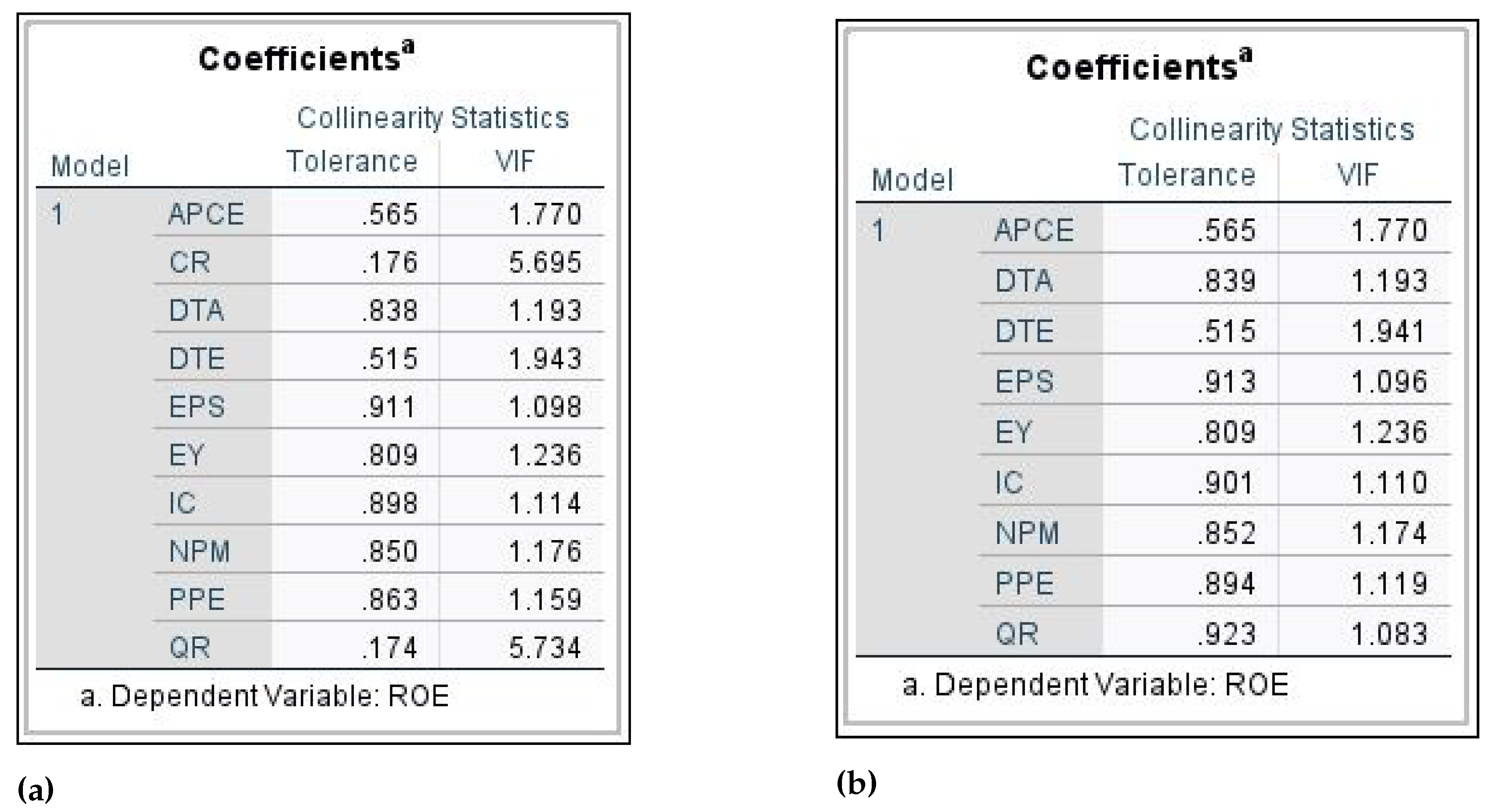
Figure 2.
ROC Curve using dataset 1.
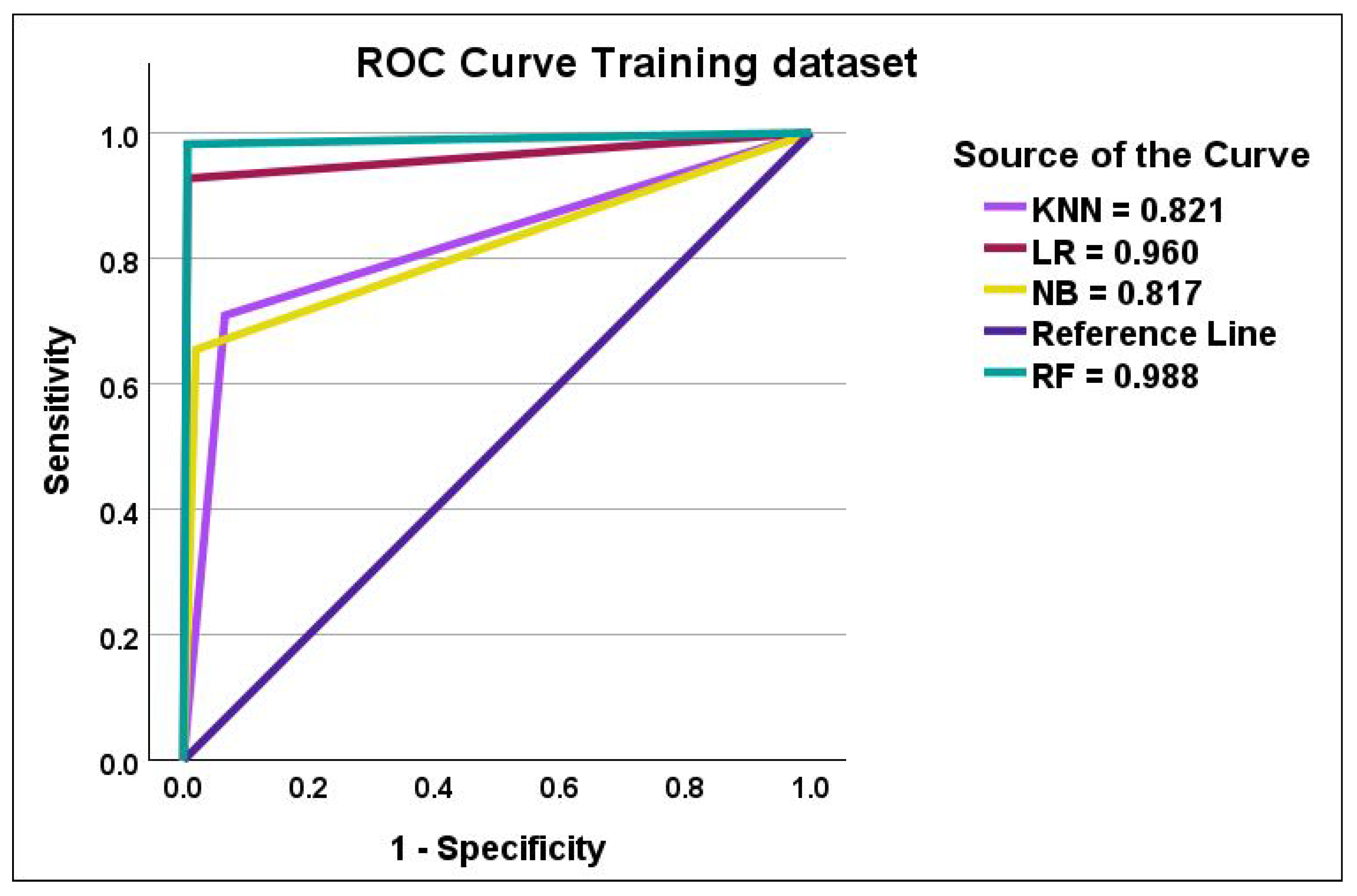
Figure 3.
Predictor selection error Log for KNN using training dataset.
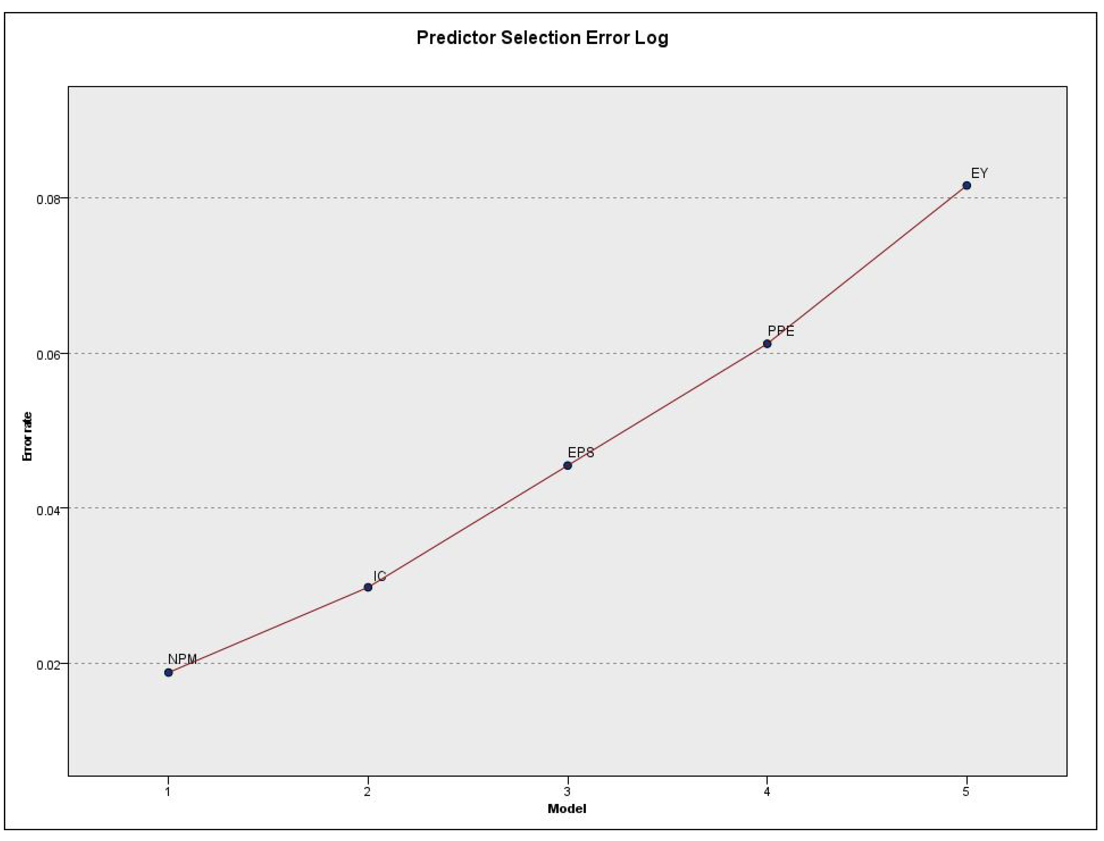
Figure 4.
Variable Selection in RF using dataset 2.
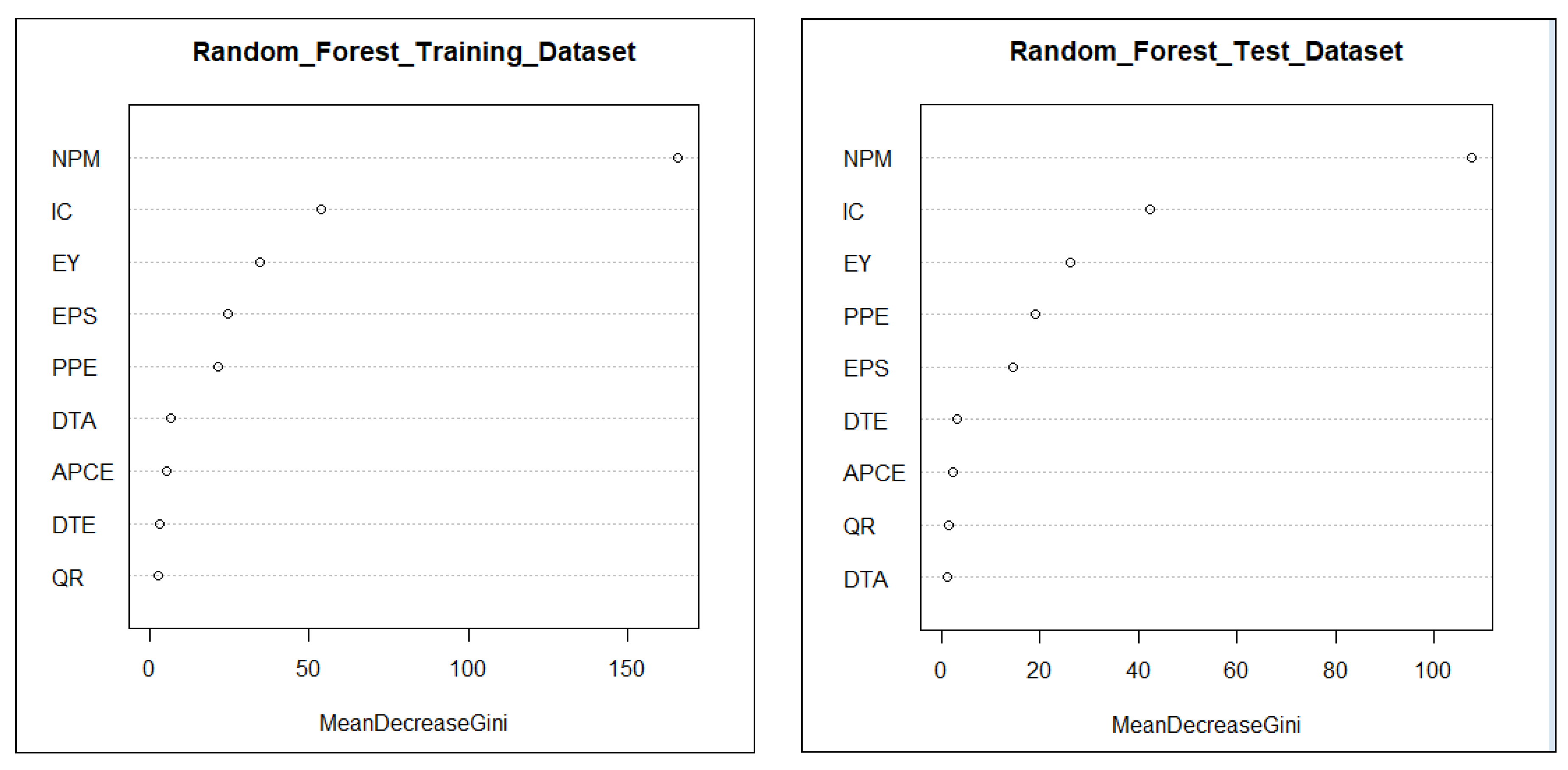
Figure 5.
Variable selection using Lasso Regression and dataset 2.
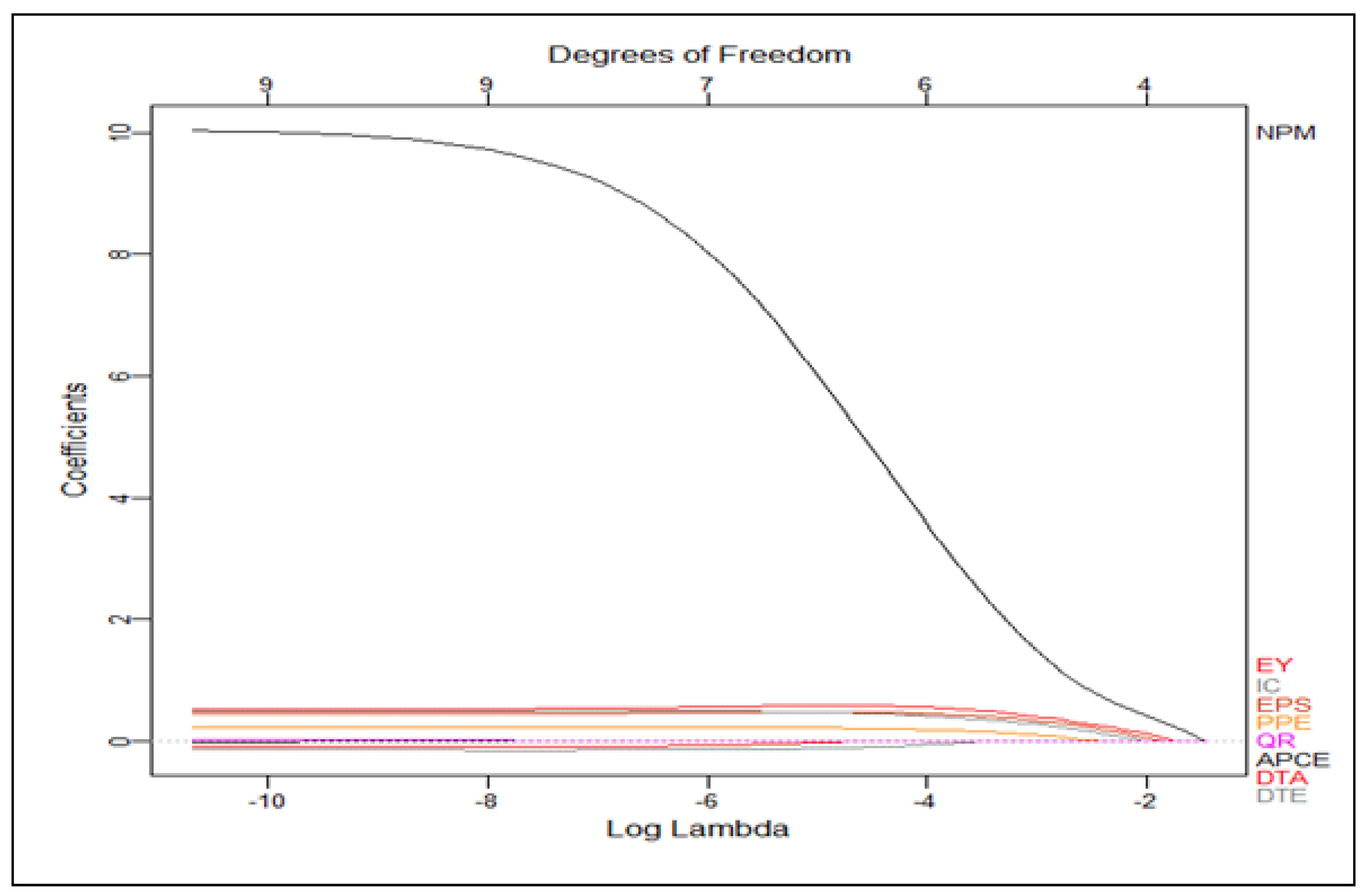
Figure 6.
Variable selection using Elastic Net Regression and dataset 2.
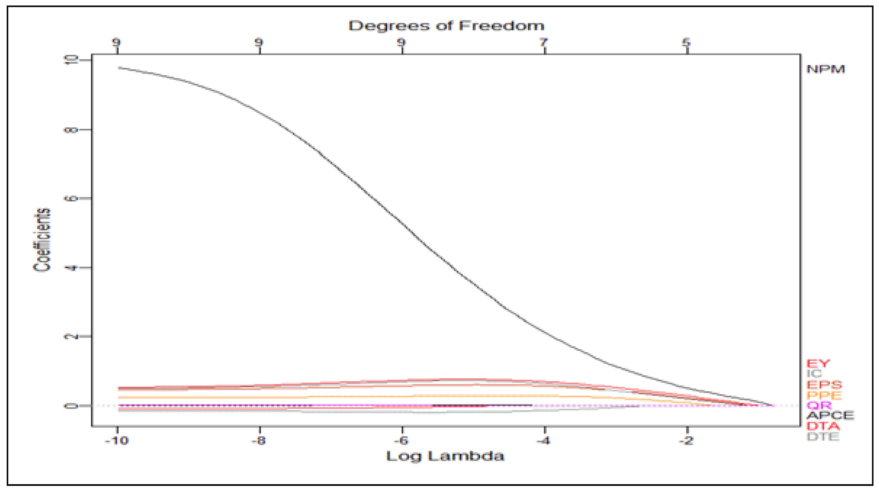
Figure 7.
Variable selection using Ridge Regression and dataset 2.
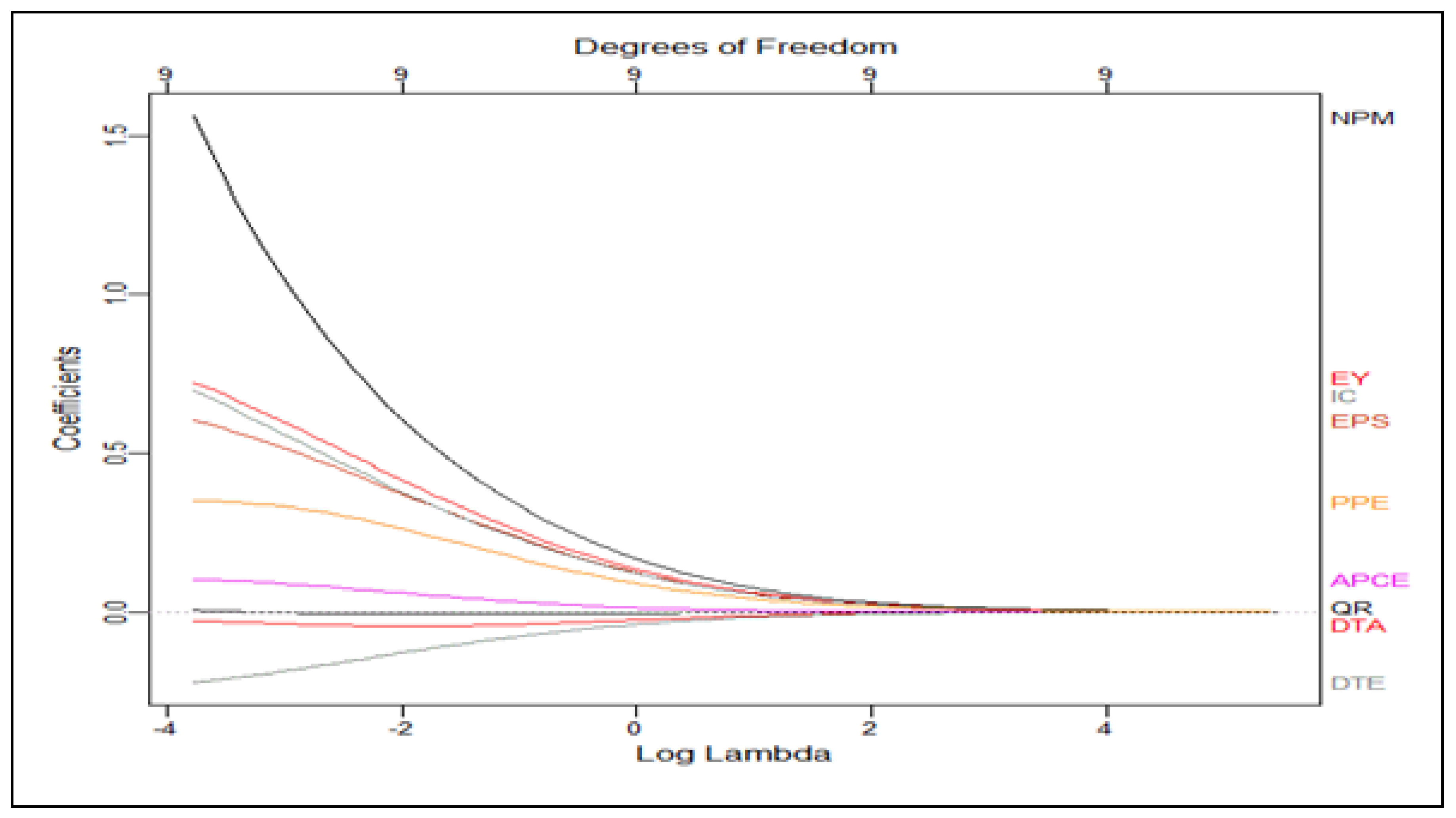
Table 1.
Classification Table.
| Predicted | Actual Class | Actual Class |
|---|---|---|
| Positive | Negative | |
| Positive | True Positive (TP) | False Positive (FP) |
| Negative | False Negative (FN) | True Negative (TN) |
Table 2.
Average Model Performance (training and test) without feature selection.
| Logistic Regresion | Naive Bayes | K Nearest Neighbour | Random Forest | |
|---|---|---|---|---|
| Sensitivity | 94.2 | 79.5 | 67.2 | 96.6 |
| Specificity | 99.2 | 98.3 | 96.8 | 98.8 |
| Precision | 97.6 | 94.5 | 87.2 | 96.6 |
| F1 Score | 95.8 | 86.3 | 75.6 | 96.6 |
| Accuracy | 97.7 | 93.2 | 89.0 | 98.2 |
| AUC | 96.9 | 86.2 | 87.1 | 99.4 |
Table 3.
Variables in the equation for LR using dataset 2.
| Variable in the Equation | |||
|---|---|---|---|
| B | Wald | Sig | |
| EPS | .001 | 4.867 | .027 |
| EY | .016 | 4.545 | .033 |
| IC | .011 | 3.263 | .071 |
| NPM | .166 | 55.596 | <.001 |
| PPE | .006 | 3.044 | .081 |
| Constant | -.047 | .118 | .731 |
Table 4.
Variable Selection in NB using dataset 2.
| Subset Summary | ||
|---|---|---|
| Subset | Predictor Added | Average Log-Likelihood |
| 1 | NPM | -.503 |
| 2 | EY | -.436 |
| 3 | IC | -.391 |
| 4 | EPS | -.360 |
| 5 | PPE | -.335 |
Table 5.
Average model performance (training and test) without feature selection.
| Logistic Regresion | Naive Bayes | K Nearest Neighbour | Random Forest | |
|---|---|---|---|---|
| Sensitivity | 92.5 | 79.1 | 84.3 | 99.1 |
| Specificity | 98.2 | 95.7 | 90.9 | 98.4 |
| Precision | 98.1 | 94.8 | 90.3 | 98.4 |
| F1 Score | 95.2 | 86.2 | 87.2 | 98.8 |
| Accuracy | 95.4 | 87.3 | 87.6 | 98.8 |
Table 6.
Average model performance (Training and Test) with feature selection.
| Logistic Regresion | Naive Bayes | K Nearest Neighbour | Random Forest | |
|---|---|---|---|---|
| Sensitivity | 91.9 | 82.0 | 91.0 | 99.3 |
| Specificity | 98.2 | 93.1 | 94.4 | 98.6 |
| Precision | 98.1 | 92.7 | 94.2 | 98.6 |
| F1 Score | 94.9 | 86.7 | 92.6 | 98.9 |
| Accuracy | 95.0 | 87.4 | 92.7 | 98.9 |
Table 7.
Average model comparison (Train and Test) without feature selection using SMOTE dataset.
| Logistic Regresion | Naive Bayes | K Nearest Neighbour | Random Forest | |
|---|---|---|---|---|
| Sensitivity | 97.6 | 85.0 | 89.5 | 99.2 |
| Specificity | 99.1 | 97.3 | 87.0 | 100 |
| Precision | 98.8 | 96.0 | 83.0 | 100 |
| F1 Score | 98.1 | 90.1 | 86.0 | 99.6 |
| Accuracy | 98.5 | 92.1 | 87.8 | 99.7 |
Table 8.
Average model comparison (Training and Test) with feature selection using SMOTE dataset.
| Logistic Regresion | Naive Bayes | K Nearest Neighbour | Random Forest | |
|---|---|---|---|---|
| Sensitivity | 97.2 | 80.5 | 90.6 | 99.2 |
| Specificity | 99.6 | 98.9 | 94.2 | 99.6 |
| Precision | 99.6 | 98.3 | 91.9 | 99.6 |
| F1 Score | 98.4 | 88.5 | 91.2 | 99.4 |
| Accuracy | 98.7 | 91.2 | 92.6 | 99.5 |
Table 11.
Average model comparison (Training and Test) with feature selection using ROSE dataset.
| Logistic Regression | p-values | Lasso Regression | Elastic Net Regression | Ridge Regression | |
|---|---|---|---|---|---|
| Intercept | 0.17840 | 0.649 | -0.86010 | -1.22162 | -1.60618 |
| APCE | -0.00789 | 0.964 | 0.00000 | 0.01630 | 0.00165 |
| DTA | -0.27335 | 0.538 | 0.00000 | -0.06427 | -0.08721 |
| DTE | -0.04230 | 0.438 | -0.09931 | -0.17304 | -0.15317 |
| EPS | 0.00126 | 0.033 | 0.47755 | 0.53806 | 0.48336 |
| EY | 0.01497 | 0.045 | 0.59205 | 0.66780 | 0.56697 |
| IC | 0.01134 | 0.063 | 0.46125 | 0.62333 | 0.53401 |
| NPM | 0.16406 | 0.001 | 5.05918 | 6.89091 | 9.08569 |
| PPE | 0.00592 | 0.070 | 0.21534 | 0.26058 | 0.24271 |
| QR | 0.00744 | 0.916 | 0.00000 | 0.03034 | 0.03298 |
Disclaimer/Publisher’s Note: The statements, opinions and data contained in all publications are solely those of the individual author(s) and contributor(s) and not of MDPI and/or the editor(s). MDPI and/or the editor(s) disclaim responsibility for any injury to people or property resulting from any ideas, methods, instructions or products referred to in the content. |
© 2026 by the authors. Licensee MDPI, Basel, Switzerland. This article is an open access article distributed under the terms and conditions of the Creative Commons Attribution (CC BY) license (http://creativecommons.org/licenses/by/4.0/).
Copyright: This open access article is published under a Creative Commons CC BY 4.0 license, which permit the free download, distribution, and reuse, provided that the author and preprint are cited in any reuse.


