

Submitted:
20 July 2026
Posted:
22 July 2026
You are already at the latest version
Abstract
The identification and delineation of subsurface resistive anomalies beneath sedimentary cover remain challenging for the magnetotelluric (MT) method. In this study, we compared the attenuation behavior of electromagnetic (EM) fields and their response characteristics under surface and/or subsurface observation configurations using both synthetic and field data. The synthetic results show that the conductive cover layer substantially suppresses the EM responses of the subsurface high resistivity body, producing only weak response perturbations at surface stations. In contrast, the response amplitudes recorded at underground stations are enhanced, indicating that underground EM observations provide advantages in resolving subsurface resistive anomalies and constraining their geometric boundaries. The results further reveal distinct attenuation behaviors of the electric and magnetic fields, with the electric field being more sensitive to variations in the bulk conductivity of the sedimentary layer. Furthermore, one-dimensional Bayesian probabilistic inversions of both synthetic and field datasets indicate that underground observations provide more robust and reliable estimates of the resistivity structure. These findings suggest that further exploration of deep underground observations and the deployment of high sensitivity quantum EM sensors have considerable potential for detecting and characterizing weak EM responses from resistive targets in sedimentary environments, while also improving the reliability of inversion results and reducing their uncertainty.
Keywords:
magnetotelluric (MT) sounding
; sedimentary cover
; electromagnetic responses
; under-ground observations
; magnetotelluric inversion
1. Introduction
Magnetotelluric (MT) sounding is one of the most widely adopted geophysical methods for investigating the deep structure of the Earth. Owing to electromagnetic (EM) attenuation and the skin effect, MT transfer functions are primarily controlled by subsurface conductive structures [1,2]. As a result, water-bearing porous media within the sedimentary cover can effectively shield the responses of underlying targets, thereby hindering their detection and inversion and giving rise to the so-called “conductive overburden” effect [2,3,4]. The inversion of conventional surface MT data is further affected by the following three factors: (1) shallow sedimentary cover significantly suppresses the EM responses of deep high-resistivity bodies, producing only minor perturbations in apparent resistivity and phase and consequently increasing inversion uncertainty [3,5]. (2) the generally strong EM noise environment encountered in surface MT observations degrades the signal-to-noise ratio of the data, thereby reducing inversion accuracy [6,7,8,9]. (3) electrical heterogeneities within near-surface sediments can induce current distortion and static-shift effects, thereby directly compromising inversion reliability [10,11].
It has been demonstrated that underground environments generally exhibit significantly lower EM background noise than surface environments [12,13,14,15]. This low-noise environment is beneficial for acquiring EM data with high signal-to-noise ratios and for capturing weak EM signals associated with deep geological processes [16]. In this study, we primarily address the question of what advantages underground observations offer over conventional surface MT observations and inversions in areas with sedimentary sequences. We employed both synthetic and field data to evaluate the potential of underground observations for improving the inversion accuracy of deep electrical structures by comparing EM responses at surface and underground stations under different sedimentary thicknesses and resistivity-anomaly configurations. In addition, for a sedimentary basin scenario, we discuss the weak EM responses of deeply buried anomalies at surface stations and the signal-detection capabilities of typical EM sensors.
2. Plane waves within Layered Model
To provide a realistic reference for the subsequent comparison and inversion of simulated and observed EM fields, we used the geological and geophysical setting of the Huainan Underground Laboratory (HNLab) to construct the synthetic model, where surface and underground EM channels were recorded synchronously. HNLab is located on the margin of the Hefei Basin in the southern North China Craton (Figure 1) and was constructed within the tunnels of the Huainan coal mine. The surface observation site is located at an elevation of +22 m, whereas the underground laboratory is situated at an elevation of −848 m. A 300–400 m thick sequence of Neogene and Quaternary sediments forms the shallow cover and unconformably overlies Mesozoic and Paleozoic coal-bearing successions composed of sandstone, mudstone, and interbedded coal seams deposited in continental and transitional marine–continental facies. The underground laboratory is hosted within the Carboniferous–Permian coal measures, with both the roof and floor strata dominated by mudstone, sandstone, and mud shale. The underlying strata comprise karstified and weathered marine Ordovician carbonates and Cambrian limestones. The logging data indicate that the overlying unconsolidated sediments have a bulk resistivity of approximately 2.2 Ω·m [16]. Wide-angle seismic data suggest that the upper-crustal cover sequence in the Hefei Basin is 4–7 km thick [17]. In addition, a broadband MT profile reveals the presence of a conductive sedimentary layer with a thickness of approximately 3–6 km [18].
2.1. Synthetic Model and Numerical Simulation
We employed a simplified one-dimensional (1D) layered resistivity model (Figure 2a) based on the stratigraphic structure and logging data shown in Figure 1. The model consists of two layers, with the upper layer represented by a conductive cover having a resistivity of 2.2 Ω·m, as constrained by the logging data [16]. Two cover thicknesses, 870 m and 5000 m, were used in the simulations. A two-dimensional resistivity model indicates that the upper crust of the Hefei Basin is characterized by resistivities of approximately 50–500 Ω·m, whereas the middle and lower crust contain large scale conductive bodies with resistivities of 10–20 Ω·m [18]. The underlying formation in our synthetic model was set as a homogeneous half space with a resistivity of 50 Ω·m.
We conducted three-dimensional (3D) forward simulations using the AC/DC Module of COMSOL Multiphysics, a finite-element-based multiphysics simulation platform [19]. The numerical model covered a computational domain of 70 km 70 km 70 km (length width height). Two orthogonal background magnetic field vectors, and , were prescribed under the plane wave assumption. The relative magnetic permeability and relative permittivity were both set to unity, and a free tetrahedral mesh was employed for spatial discretization. To minimize the effects of frequency-dependent mesh resolution and finite-domain boundary conditions, only the effective frequency range of the simulated data was considered in the following analysis. In addition, the resistivity of the underlying layer in Figure 2a was assigned values of 2.2, 50, and 500 Ω·m. The ratios between the EM fields at the surface and those at depth were then calculated using a recursion formulation based on 1D layered earth theory [4,20]. Stations were placed at the surface and at the base of the sedimentary layer, and the corresponding ratios of surface to underground EM fields are presented in Figure 2b and Figure 2c.
2.2. Results and Analysis
A comparison of the surface and underground EM fields obtained from different simulation methods and field measurements, as shown in Figure 2, reveals the following:
- (1)
- The 3D forward modeling results agree well with those derived from the recursion method at frequencies below 10 Hz for the 870 m thick sedimentary layer and below 3 Hz for the 5000 m thick sedimentary layer. Notably, the 3D simulated responses become distorted in higher-frequency bands because of frequency-dependent mesh-resolution limitations. The measured magnetic field at a depth of 870 m shows good agreement with the simulated results, whereas the attenuation coefficient of the measured electric field is lower than that predicted by the simulations. This discrepancy is probably attributable to the fact that the study area deviates from an ideal 1D layered earth model. In addition, the difficulty of positioning electrodes at underground stations is likely an important factor contributing to the differences between the measured and simulated results.
- (2)
- The electric and magnetic fields exhibit different attenuation coefficients. For example, when 50 Ω·m, the electric field attenuation coefficients for sedimentary-layer thicknesses of 5000 m and 870 m are approximately 0.002 and 0.5 at 1 Hz, 0.2 and 1 at 0.1 Hz, and both approach unity at 0.01 Hz, respectively. In contrast, the corresponding magnetic field attenuation coefficients are approximately 0.001 and 0.1 at 1 Hz, 0.04 and 0.3 at 0.1 Hz, and 0.2 and 0.6 at 0.01 Hz, respectively. These results indicate that: (i) for a given sedimentary layer thickness, the magnetic field is more strongly attenuated than the electric field; and (ii) increasing sedimentary layer thickness enhances electric field attenuation more markedly in the high frequency band, whereas its influence on magnetic field attenuation persists over a broader low frequency band.
- (3)
- The electric field attenuation curves for different values of are relatively similar, whereas the magnetic field attenuation curves exhibit more pronounced differences. This indicates that, under the influence of shallow sedimentary layers, the magnetic field response is more sensitive to resistivity perturbations in the background medium.
3. Inversion of Layered Models
To further investigate the effects of shallow sedimentary cover on the apparent resistivity, impedance phase, and inversion results of surface and underground MT observations, we performed 1D MT inversion for both synthetic and field data using the trans-dimensional Markov chain Monte Carlo (RJMCMC) algorithm [21]. This method does not require the number of model layers to be specified a priori, and statistical analysis of the probability distributions of the inversion results provides a better characterization of the non-uniqueness and uncertainty associated with different datasets.
3.1. Synthetic Data
Figure 3a and Figure 3b present the apparent resistivity and impedance phase curves of the layered model shown in Figure 2(a) for observations at the surface and at a depth of 870 m, respectively. For the surface station, the apparent resistivity remains approximately 2.2 Ω·m over the frequency range of 10,000–1 Hz, while the impedance phase is close to 45°. At longer periods of T > 1 s, the apparent resistivity gradually increases, reaching approximately 20 Ω·m at T = 100 s, while the corresponding impedance phase gradually decreases. In contrast, at the underground station, the apparent resistivity remains approximately 50 Ω·m and the impedance phase remains close to 45° over the entire frequency range. The sounding data from the underground station better characterize the resistivity properties of the underlying basement. It should be noted that, owing to frequency-dependent mesh-resolution limitations in our AC/DC Module simulations, extrapolation was used to supplement the high frequency data for both surface and underground stations. Specifically, for the surface data, the skin depths associated with the supplemented high frequency responses are smaller than the thickness of the sedimentary layer; therefore, these responses have a negligible influence on the delineation of resistivity interfaces. For the underground data, because the basement is assumed to be a homogeneous medium with uniform resistivity, the supplemented high-frequency data likewise do not introduce spurious interface anomalies. Therefore, extrapolation of the high-frequency data has no significant influence on the inversion results.
The 1D inversion results for the surface and underground data are presented in Figure 3c and Figure 3d, respectively. Both inversions achieve good data fits (Figure 3a and Figure 3b) and recover the subsurface resistivity structure. The results for the surface station indicate that the posterior probability distribution of shallow resistivity is highly concentrated, suggesting that the inversion provides strong constraints on the shallow sedimentary layer. However, the estimated thickness of the sedimentary layer shows a certain deviation from the true value. In addition, although the mode and median models are broadly consistent with the true resistivity at greater depths, the mean model yields resistivities higher than the true values. Moreover, the interval between the 10th and 90th percentile models spans several orders of magnitude, ranging from 50 Ω·m to several tens of thousands of Ω·m, reflecting the uncertainty in the inversion results. In contrast, all probabilistic models obtained from the underground station are tightly clustered around the true values, demonstrating good inversion reliability and accuracy.
We further added Gaussian noise to the sounding data shown in Figure 3 to assess the robustness of the inversions. The mean of the Gaussian noise was set to zero for both apparent resistivity and impedance phase, while the standard deviations were set to 10 Ω·m and 5°, respectively. Because of the dominant influence of the shallow conductive sedimentary layer on bulk resistivity, the apparent resistivity at the surface station is generally low in the high-frequency band. As a result, even minor noise perturbations may lead to substantial deviations in apparent-resistivity amplitudes. By comparison, the apparent resistivity at the underground station is less sensitive to the same level of noise.
Figure 4 shows the noisy data and corresponding inversion results. Although the apparent resistivity curves of the surface data differ considerably before and after noise contamination, the model responses remain close to the noise free data (Figure 4a). By comparison, the phase data are less affected by noise, resulting in a better data fit (Figure 4b). For the underground station, the apparent-resistivity response fitted to the noisy data is generally consistent with the noise free data, except for slightly higher amplitudes in the low frequency band. The phase data also exhibit an excellent fit. The inversion results for the surface station exhibit highly dispersed posterior probability distributions at depths of approximately 700–3000 m, indicating a high degree of uncertainty in the inverted models. Furthermore, the resistivities of both the mode and median models exceed 1000 Ω·m, representing a substantial departure from the true model. In contrast, despite the relatively large interval between the 10th and 90th percentile models, the results from the underground station are considerably more concentrated. The mode model agrees well with the true model, while the median and mean models also reproduce the true structure reasonably well, with the main deviations confined to depths between 1000 and 1500 m. These results further demonstrate that, for noise contaminated data, inversion based on underground observations provides higher reliability and lower uncertainty than inversion based on surface observations.
3.2. Field Data
We further conducted 1D inversion using synchronously observed surface and underground MT data from HNLab. A total of 24 hours data were selected for impedance tensor estimation. During the observations, HNLab was still undergoing planning, design, and renovation. Therefore, both surface and underground data were affected by EM noise to varying degrees, including noise from high voltage transmission facilities, power supply systems, ventilation and drainage equipment, railway transport systems, mine hoists, and densely distributed pumping pipelines. Figure 5 shows a comparison of the apparent resistivity and phase data obtained from the surface and underground stations.
- (1)
- In the frequency band of > 10 Hz, both apparent resistivity and phase curves of the ground station exhibit considerable outlier (Figure 5a, blue shaded region). Although the underground apparent resistivity curves are relatively continuous, the phase data exhibit out-of-quadrant behavior, and the YX-mode phase curve is distorted (Figure 5b, blue shaded region). This indicates strong attenuation of high frequency EM fields by the overlying conductive layer, resulting in significant distortions in impedance estimation when conventional MT processing approaches are used.
- (2)
- In the 10–1000 s period band, the overall quality of the surface data improves; however, the YX-mode data still exhibit obvious outliers. By contrast, the underground data are smoother and more continuous. However, in the 10–100 s period band, the underground phase curve transitions from out-of-quadrant behavior toward values close to 45° or −135°, indicating that attenuation by the shallow sedimentary layer still affects the data in this band and leads to biased transfer functions.
- (3)
- At periods longer than 1000 s, the surface apparent resistivity curve exhibits an upward trend with an approximately 45° slope, suggesting that the data are significantly affected by near-field effects (Figure 5a, orange-shaded region). In contrast, the underground data appear to be free from surface near-field sources. The data quality remains generally good up to a period of 10,000 s, except for some outliers at low frequencies (Figure 5b, orange-shaded region).
Figure 6 shows the 1D inversion results for the surface and underground observations. Considering the effects of high frequency noise and low frequency near-field effects, data in the period range of 1–3000 s were used. In addition, attenuation by the shallow sedimentary layer causes distortion of the underground transfer functions in the high frequency range. Therefore, inversion results obtained with and without retaining the out-of-quadrant period range of 1–200 s were further compared. The results suggest the following:
- (1)
- The results derived from the surface data indicate a low resistivity layer (~1 Ω·m) at depths shallower than 1 km, consistent with the characteristics of the shallow sedimentary layer. However, the resistivity increases sharply to ~10,000 Ω·m below 1 km, resulting in a complete loss of resolution for deeper structures (Figure 6c).
- (2)
- The interval between the 10th and 90th percentile models derived from the underground data is relatively wide, indicating low model certainty. The phase fit is poor when the distorted high-frequency band is included (Figure 6b). The results indicate resistivities of ~1000 Ω·m at depths of 1–5 km, decreasing to ~10 Ω·m at 5–12 km and increasing again to ~1000 Ω·m at 12–22 km. The subsurface is characterized by a low-resistivity feature of approximately 10 Ω·m below a depth of ~22 km (Figure 6d). We suggest that the out-of-quadrant distortions in the high frequency band are responsible for the two high resistivity layers imaged in the inversion models.
- (3)
- The results obtained using only the low frequency underground data (Figure 6e) indicate that the probabilistic models are dispersed at depths shallower than ~8 km. This is likely due to the lack of high frequency data constraints. Model uncertainty is relatively reduced below 8 km. The mode and median models indicate a simple subsurface structure with a resistivity of approximately 10 Ω·m. The mean model shows a decrease in resistivity from several tens of Ω·m at depths of 8–15 km to ~20 Ω·m at depths of 15–40 km, followed by a further decrease to ~10 Ω·m below a depth of ~40 km. This result is broadly consistent with previous evidence for a large scale mid- to lower-crustal conductive layer [18].
Overall, in contrast to the severely distorted results derived from the surface data, the underground data still provide effective constraints on deep resistivity structures to some extent, although both surface and underground data were affected by strong and complex EM noise. This demonstrates that underground observations have advantages in improving inversion results by mitigating the influence of shallow sediments.
4. Surface Electromagnetic Response Controlled by Sedimentary Cover
Identifying and extracting the weak responses of deep high resistivity targets remain challenging in terms of observation configuration, instrumentation, and data processing, particularly because of the shielding effect of a conductive cover layer. Figure 7 shows a 3D resistivity model consisting of a shallow conductive overburden (2.2 Ω·m) overlying a 50 Ω·m basement. A 3D high resistivity body was embedded in the model, with its top located at a depth of 30 km and dimensions of 30 km 30 km 20 km (length width height). An MT profile was deployed at the center of the model surface. 3D forward simulations were performed using the COMSOL AC/DC Module to investigate the EM response characteristics of the resistive anomaly at surface and underground stations.
Figure 8 shows the variations in electric-field response along the profile deployed at the surface. The amplitudes at the center of the profile indicate the following:
- (1)
- For a sedimentary layer thickness of 870 m, the response induced by the 1000 Ω·m anomaly exceeds 200 mV/km at T = 10,000 s, whereas that induced by the 55 Ω·m anomaly is close to 20 mV/km (Figure 8a). The response induced by the 55 Ω·m anomaly still reaches several tens of mV/km at T = 10 s (Figure 8d). However, the electric-field response induced by the 1000 Ω·m anomaly is only 0.016 mV/km at T = 1 s (Figure 8e), whereas the self-noise level of conventional non-polarizable electrodes is 0.01 mV/km/√Hz at 1 Hz [22]. This indicates that conventional non-polarizable electrodes may have difficulty for reliably detecting such weak signals.
- (2)
- For a sedimentary layer thickness of 5000 m, the 1000 Ω·m anomaly induces a response exceeding 50 mV/km at T = 10,000 s, whereas the response induced by the 55 Ω·m anomaly is approximately 5 mV/km (Figure 8a). Compared with the self-noise level of conventional non-polarizable electrodes, which is approximately 1 mV/km/ at 1 mHz [22], the electric-field response induced by the 55 Ω·m anomaly at the surface is relatively weak. For T < 100 s, the results show negative amplitudes (Figure 8c–e), probably because the skin depth is smaller than the depth to the top of the target.
Compared with the electric-field response, the magnetic-field response is weaker because induced eddy currents are suppressed within high resistivity anomalies. Figure 9 shows the variations in magnetic-field response along the profile, indicating the following:
- (1)
- The magnetic-field responses for sedimentary-layer thicknesses of 870 m and 5000 m are nearly identical at T = 10,000 s (Figure 9a), indicating that variations in sedimentary-layer thickness have only a limited influence on long period magnetic-field induction. When the anomaly resistivity is 1000 Ω·m, the amplitude difference between the profile center and the profile boundary exceeds 0.1 nT, whereas for the 55 Ω·m anomaly, it is less than 0.01 nT. The self-noise level of typical magnetic sensors > 1 nT/ at T = 10,000 s [22] is insufficient for resolving the response characteristics described above.
- (2)
- (3)
- At T = 1 s, the response difference between the profile center and boundary for the 1000 Ω·m anomaly is only 1.4 pT and 5 aT for sedimentary layer thicknesses of 870 m and 5000 m, respectively (Figure 9e). The former is already close to the theoretical noise level of conventional induction coils, which is approximately 1 pT/at 1 Hz [22]. The latter is far below the noise level of low temperature superconducting magnetometers, which is approximately 1 fT/ at 1 Hz [23].
The results indicate that the magnetic-field response is relatively insensitive to high resistivity medium. Under the influence of a conductive sedimentary cover, the surface magnetic-field response of subsurface structures is further attenuated, imposing stricter requirements on background noise levels and the sensitivity of magnetic sensors.
The apparent resistivity responses (Figure 10) and electric-field responses (Figure 8) exhibit consistent curve characteristics, indicating that the apparent resistivity response of the deep high resistivity anomaly is primarily controlled by the electric-field response.
- (1)
- For a sedimentary layer thickness of 870 m, the relative apparent resistivity response of the 1000 Ω·m anomaly is approximately 0.03 Ω·m at T = 10,000 s, 0.6 Ω·m at T = 1000 s, and 0.3 Ω·m at T = 100 s (Figure 10a–c).
- (2)
- For a sedimentary layer thickness of 5000 m, the relative apparent-resistivity response remains very weak across the entire period range.
Overall, the responses of deep high-resistivity anomalies in surface MT observations are relatively weak, indicating that surface observation configurations generally have difficulty on constraining the geometric boundaries of deep 3D high resistivity bodies beneath a conductive sedimentary cover. On the other hand, how to use inversion algorithms to retrieve the electrical structure implied by the responses, and how to improve the determinacy, uniqueness, and reliability of anomaly resistivity values and boundary information in inversion results, are beyond the scope of this study.
5. Discussion
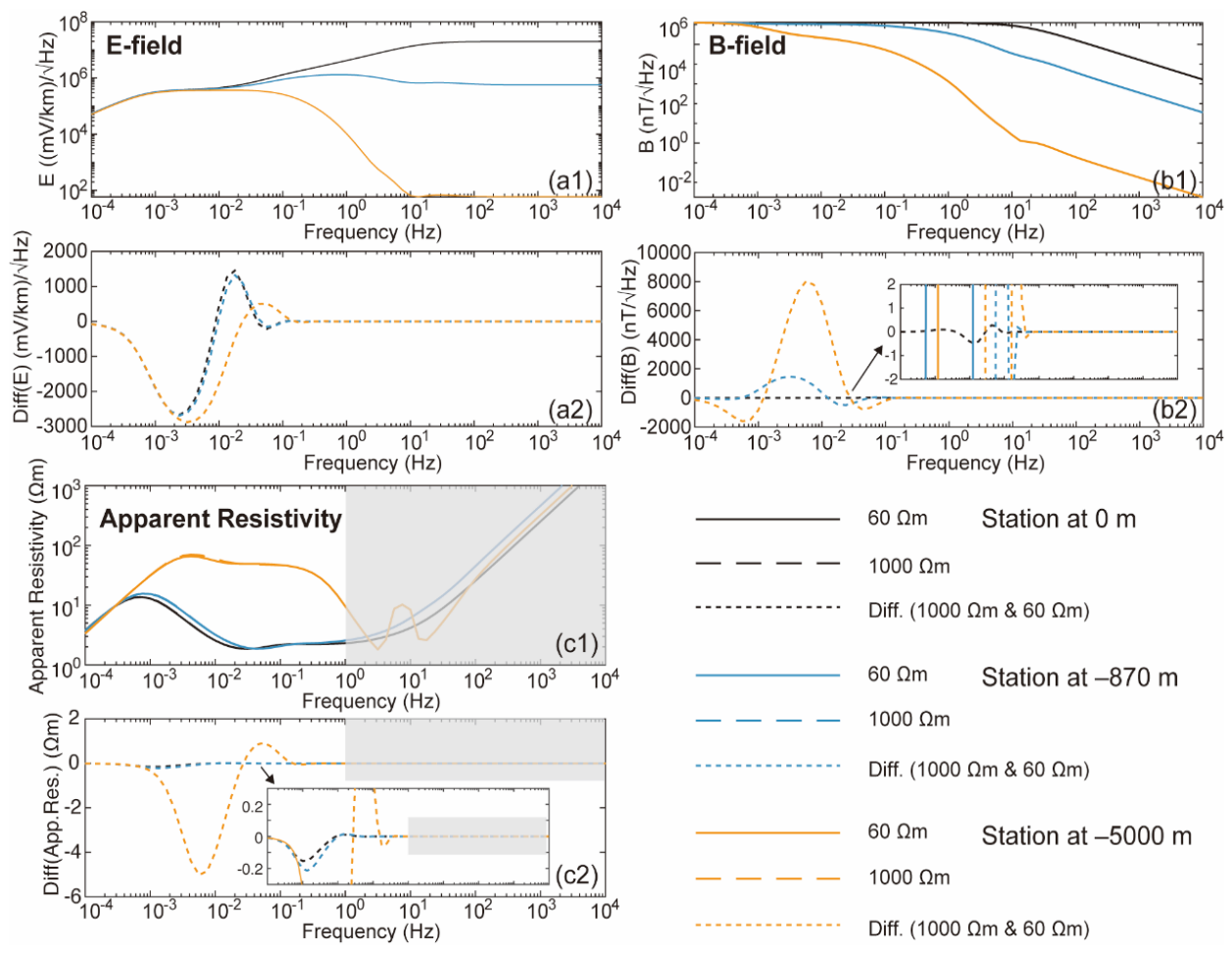
Figure 11 shows the electric-field, magnetic-flux-density, and apparent resistivity curves for surface and underground stations deployed at different depths, as well as the response differences in these physical quantities for different anomalies. The results show that the EM responses at observation sites with different depths exhibit significant differences, as indicated by the curves of different colors in Figure 11a1, Figure 11b1, and Figure 11c1. In contrast, for anomalies with different resistivities, the EM field and apparent resistivity response curves at the same depth are nearly identical, as indicated by the solid and long-dashed lines in Figure 11a1, Figure 11b1, and Figure 11c1. This suggests that the resistivity contrasts of deep anomalies, such as 60 Ω·m and 1000 Ω·m, produce only very weak perturbations at the observation sites. The comparison between surface and underground EM fields indicates the following:
- (1)
- (2)
- (3)
- The magnetic-field differences at the surface are very weak (<1 nT), whereas the maximum amplitude approaches 2000 nT at 0.004 Hz at a depth of −870 m. The maximum amplitude further increases to 8000 nT at 0.006 Hz at a depth of −5000 m (Figure 11b2).
- (4)
- Compared with the results from the surface and a depth of −870 m, the apparent-resistivity response at a depth of −5000 m better reflects the characteristics of the deep high-resistivity medium (Figure 11c1). In addition, the apparent-resistivity differences are only approximately 0.2 Ω·m at the surface and at a depth of −870 m, whereas the difference increases to 5 Ω·m at a depth of −5000 m (Figure 11c2). Clearly, the perturbation signatures associated with resistivity contrasts in high resistivity bodies are more pronounced in deeper underground observations, particularly at −5000 m.
6. Conclusions
Our study focuses on the EM response behavior under the influence of shallow sedimentary cover. Using both synthetic and field data, we compare the attenuation characteristics of EM fields and the corresponding 1D probabilistic inversion models. We discuss the controlling effect of sedimentary cover on the EM responses of underlying high-resistivity anomalies in surface and underground observations.
- (1)
- The electric and magnetic fields differ in their attenuation behavior and attenuation coefficients during propagation through shallow sediments, with the conductive layer exerting a more pronounced attenuation effect on the magnetic field. In contrast, electric field perturbations are more sensitive to variations in sedimentary layer thickness. The 1D probabilistic inversion results for both synthetic and field data indicate that models derived from underground observations exhibit higher certainty and reliability.
- (2)
- Under the influence of a shallow conductive layer, the EM field and transfer function responses associated with deep high resistivity anomalies are relatively weak in surface data. The limited sensitivity of conventional EM sensors makes it difficult to identify high frequency perturbation features and further constrain the boundaries of high resistivity targets.
- (3)
- Variations in the resistivity of resistive anomalies produce only weak response perturbations in surface and shallow underground observations, whereas the responses are enhanced in deeper underground data. We suggest that deep underground observations have potential advantages for improving the accuracy and reliability of modeling deep high resistivity bodies.
- (4)
- For underground observations, transfer functions in the high frequency band derived using conventional data processing methods are distorted and should be excluded from data analysis and inversion. Alternatively, inversion approaches based on integrated surface–underground full space observation systems should be developed.
Author Contributions
Conceptualization, C.X., Y.T. and Y.W.; methodology, C.X. and Y.T.; software, Y.T. and Z.Z.; validation, C.X. and Y.T.; formal analysis, C.X., Y.T. and Y.W.; investigation, C.X., Y.T., Z.Z. and Y.W.; data curation, Y.T.; writing—original draft preparation, C.X. and Y.T.; writing—review and editing, C.X., Y.T. and Y.W. All authors have read and agreed to the published version of the manuscript.
Funding
This research was funded by the National Science and Technology Major Project for Deep Earth Probe and Mineral Resources Exploration, grant number 2024ZD1002702, and the National Natural Science Foundation of China, grant numbers 42474111 and 42074083.
Data Availability Statement
The datasets generated during the current study are publicly avail-able in the Zenodo repository: https://doi.org/10.5281/zenodo.21149601.
Acknowledgments
We extend our gratitude to the Huaihe Energy Company Limited for providing safety guarantees and equipment maintenance during the underground observations. We thank the employees and students from the China University of Geosciences (Beijing) who participated in the field experiments. We used the high-performance computing facilities at China University of Geosciences (Beijing) for data processing. We used the COMSOL Multiphysics® software to perform the synthetic forward modeling.
Conflicts of Interest
The authors declare no conflicts of interest.
References
- Lin, W.; Yang, B.; Han, B.; Hu, X. A Review of Subsurface Electrical Conductivity Anomalies in Magnetotelluric Imaging. Sensors 2023, 23, 1803.
- Simpson, F.; Bahr, K. Practical Magnetotellurics; Cambridge University Press: Cambridge, 2005.
- Nabighian, M.N. Electromagnetic Methods in Applied Geophysics: Volume 2, Application, Parts A and B; Society of Exploration Geophysicists: 1991.
- Schmucker, U. Anomalies of geomagnetic variations in the Southwestern United States. 1970.
- N., N.M.; Corbett, J.D. Electromagnetic Methods in Applied Geophysics: Volume 1, Theory; Society of Exploration Geophysicists: 1987.
- Zhao, G.Z.; Zhang, X.M.; Cai, J.T.; Zhan, Y.; Ma, Q.Z.; Tang, J.; Du, X.B.; Han, B.; Wang, L.F.; Chen, X.B.; et al. A review of seismo-electromagnetic research in China. Science China Earth Sciences 2022. [CrossRef]
- Jones, A.G.; Chave, A.D.; Egbert, G.; Auld, D.; Bahr, K. A comparison of techniques for magnetotelluric response function estimation. Journal of Geophysical Research: Solid Earth 1989, 94, 14201-14213. [CrossRef]
- Chave, A.D.; Thomson, D.J.; Ander, M.E. On the robust estimation of power spectra, coherences and transfer functions. Journal of Geophysical Research: Solid Earth 1987, 92, 633–648. [CrossRef]
- Egbert, G.D. Robust multiple-station magnetotelluric data processing. Geophysical Journal International 1997, 130, 475-496.
- Bahr, K. INTERPRETATION OF THE MAGNETOTELLURIC IMPEDANCE TENSOR - REGIONAL INDUCTION AND LOCAL TELLURIC DISTORTION. Journal of Geophysics-Zeitschrift Fur Geophysik 1988, 62, 119-127.
- Bahr, K. Galvanic Distortion. In Encyclopedia of Geomagnetism and Paleomagnetism, Gubbins, D., Herrero-Bervera, E., Eds.; Springer Netherlands: Dordrecht, 2007; pp. 277-278.
- Ren, H.; Wang, Y.; Chen, C.; Fu, G.; Qiu, L.; Guo, L.; Xie, C.; He, Y.; Sun, H.; Teng, J. Underground laboratories · Deep underground observation · Scientific questions—Insights from observations of multi-physic fields in deep underground labs. Science China Earth Sciences 2025, 68, 343-362. [CrossRef]
- Guo, L.; Wang, B.; Song, X.; Wang, Y.; Jin, C.; Yao, S.; Shi, Y. Continuous observation of geomagnetic total-field at the underground laboratory in Huainan city, China and its time-varying characteristics. Chinese Journal of Geophysics 2024, 67, 820-828. [CrossRef]
- Wang, Y.; Yang, Y.; Sun, H.; Xie, C.; Zhang, Q.; Cui, X.; Chen, C.; He, Y.; Miao, Q.; Mu, C.; et al. Observation and research of deep underground multi-physical fields-Huainan -848 m deep experiment. Sci China Earth Sci 2023, 66, 54-70. [CrossRef]
- Wang, Y.; Jian, Y.F.; He, Y.S.; Miao, Q.Q.; Teng, J.W.; Wang, Z.M.; Rong, L.L.; Qiu, L.Q.; Xie, C.L.; Zhang, Q.S.; et al. Underground laboratories and deep underground geophysical observations. Chinese Journal of Geophysics 2022, 65, 4527-4542. [CrossRef]
- Xie, C.; Chen, C.; Liu, C.; Wan, W.; Jin, S.; Ye, G.; Jing, J.; Wang, Y. Insights from underground laboratory observations: attenuation-induced suppression of electromagnetic noise. The European Physical Journal Plus 2024, 139, 218. [CrossRef]
- Xu, T.; Zhang, Z.J.; Tian, X.; Liu, B.F.; Bai, Z.; Lü, Q.; Teng, J.W. Crustal structure beneath the Middle-Lower Yangtze metallogenic belt and its surrounding areas: Constraints from active source seismic experiment along the Lixin to Yixing profile in East China. Acta Petrologica Sinica 2014, 30, 918-930.
- Qiang, J.K.; Wang, X.Y.; Tang, J.T.; Pan, W.; Zhang, Q.J. The geological structures along Huainan-Liyang magnetotelluric profile: Constraints from MT data. Acta Petrologica Sinica 2014, 30, 957-965.
- COMSOL Multiphysics® 6.4; COMSOL AB: Stockholm, Sweden, 2025.
- Constable, S.; Orange, A.; Hoversten, G.; Morrison, H. Marine magnetotellurics for petroleum exploration Part I: A sea-floor equipment system. Geophysics 1998, 63. [CrossRef]
- Brodie, R.C.; Jiang, W. Trans-dimensional Monte Carlo inversion of short period magnetotelluric data for cover thickness estimation. ASEG Extended Abstracts 2018, 2018, 1-7.
- Tian, Y.; Wan, W.; Qiao, S.; Zhang, Z.; Chen, C.; Xie, C. Self-noise modeling of electromagnetic sensors using M-estimation and multi-channel correlation analysis. Chinese Journal of Geophysics 2026, 69, 1323-1334. [CrossRef]
- Stolz, R.; Schmelz, M.; Zakosarenko, V.; Foley, C.; Tanabe, K.; Xie, X.; Fagaly, R.L. Superconducting sensors and methods in geophysical applications. Superconductor Science Technology 2021, 34, 033001. [CrossRef]
Figure 1.
Regional geological and geophysical setting of the study area and the locations of the observation sites, modified from [16]. (a) Location of the Huainan Underground Laboratory; (b) borehole log column for the depth interval of 800–900 m, indicated by the red dashed frame in panel (c); (c) logging curves; (d) locations of the surface and underground MT stations.
Figure 1.
Regional geological and geophysical setting of the study area and the locations of the observation sites, modified from [16]. (a) Location of the Huainan Underground Laboratory; (b) borehole log column for the depth interval of 800–900 m, indicated by the red dashed frame in panel (c); (c) logging curves; (d) locations of the surface and underground MT stations.
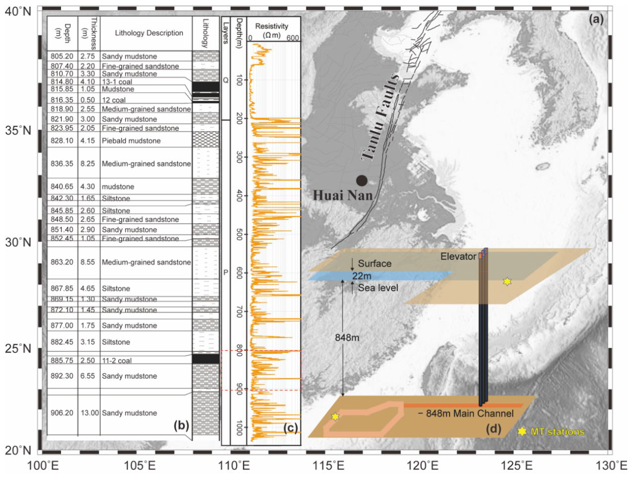
Figure 2.
Ratios between EM-field responses at surface and underground stations. (a) Resistivity model with a sedimentary layer resistivity of 2.2 Ω·m and cover thicknesses of 870 m and 5000 m. The cover layer is underlain by a homogeneous medium with resistivities of 2.2, 50, and 500 Ω·m. Stations are located at the surface and at the base of the sedimentary layer. (b) Underground-to-surface ratio of the electric field. (c) Underground-to-surface ratio of the magnetic field. Solid lines indicate the results for the 870 m thick sedimentary layer, whereas dashed lines indicate those for the 5000 m thick sedimentary layer. Black, light-blue, and dark-blue curves denote the theoretical results calculated using the recursion formulation [4,20] for 2.2, 50, and 500 Ω·m, respectively. Red curves denote the finite-element-based 3D simulation results for 50 Ω⋅m, with gray segments indicating distorted frequency bands. Orange curves represent the observed results in HNLab, using only the Ex and Bx components.
Figure 2.
Ratios between EM-field responses at surface and underground stations. (a) Resistivity model with a sedimentary layer resistivity of 2.2 Ω·m and cover thicknesses of 870 m and 5000 m. The cover layer is underlain by a homogeneous medium with resistivities of 2.2, 50, and 500 Ω·m. Stations are located at the surface and at the base of the sedimentary layer. (b) Underground-to-surface ratio of the electric field. (c) Underground-to-surface ratio of the magnetic field. Solid lines indicate the results for the 870 m thick sedimentary layer, whereas dashed lines indicate those for the 5000 m thick sedimentary layer. Black, light-blue, and dark-blue curves denote the theoretical results calculated using the recursion formulation [4,20] for 2.2, 50, and 500 Ω·m, respectively. Red curves denote the finite-element-based 3D simulation results for 50 Ω⋅m, with gray segments indicating distorted frequency bands. Orange curves represent the observed results in HNLab, using only the Ex and Bx components.
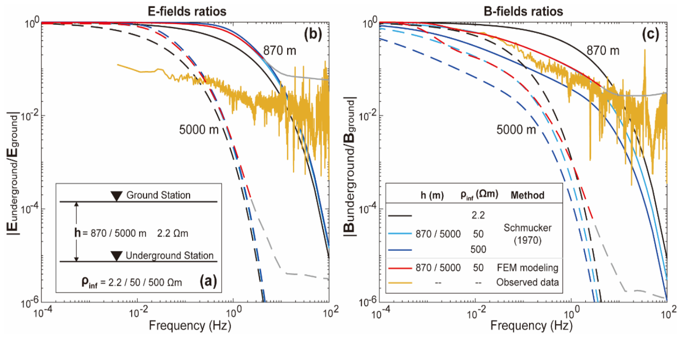
Figure 3.
Synthetic sounding data and corresponding 1D inversion results. (a) Apparent resistivity curves; (b) phase curves. The red dots and blue solid lines denote the synthetic data at the surface station and the corresponding model responses, respectively. The orange dots and light-blue solid lines denote the synthetic data at a depth of 870 m and the corresponding model responses, respectively. (c, d) 1D inversion results for the surface and underground stations, respectively. The red solid line denotes the median model; the red dashed lines denote the 10th and 90th percentile models; the blue solid line denotes the mean model; and the green solid line denotes the mode model.
Figure 3.
Synthetic sounding data and corresponding 1D inversion results. (a) Apparent resistivity curves; (b) phase curves. The red dots and blue solid lines denote the synthetic data at the surface station and the corresponding model responses, respectively. The orange dots and light-blue solid lines denote the synthetic data at a depth of 870 m and the corresponding model responses, respectively. (c, d) 1D inversion results for the surface and underground stations, respectively. The red solid line denotes the median model; the red dashed lines denote the 10th and 90th percentile models; the blue solid line denotes the mean model; and the green solid line denotes the mode model.
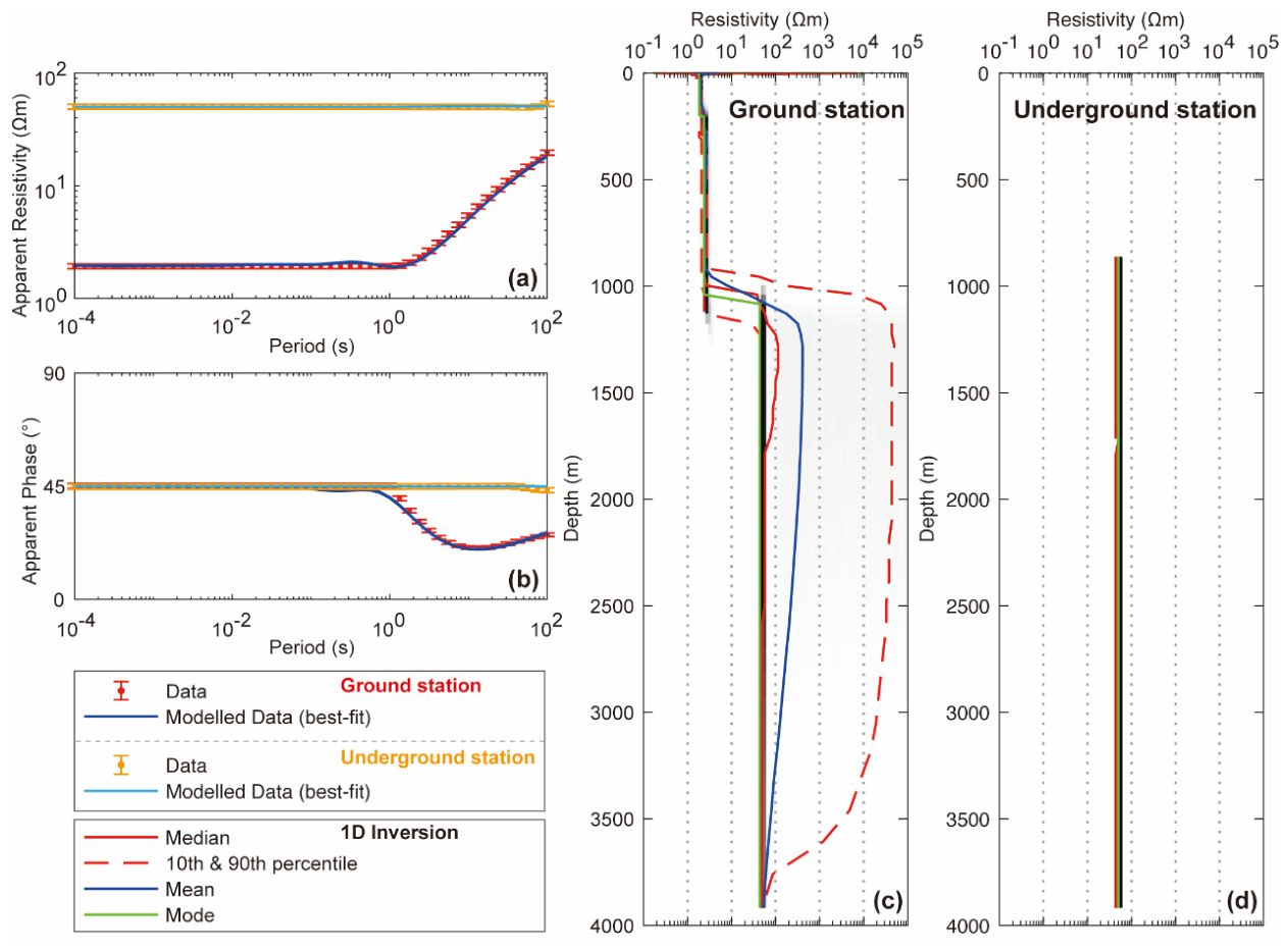
Figure 4.
Noise contaminated synthetic sounding data and corresponding 1D inversion results. (a) Apparent resistivity curves; (b) phase curves. Red and gray dots represent the noise free, and noise contaminated synthetic data at the surface station, respectively. The blue solid lines denote the model responses fitted to the noisy surface data. The orange and brown dots represent the noise free, and noise contaminated synthetic data at the underground station, respectively. The light-blue solid lines denote the model responses fitted to the noisy underground data. (c, d) Posterior probability statistics of the 1D inversion models for the surface and underground stations, respectively. The red solid line denotes the median model; the red dashed lines denote the 10th and 90th percentile models; the blue solid line denotes the mean model; and the green solid line denotes the mode model.
Figure 4.
Noise contaminated synthetic sounding data and corresponding 1D inversion results. (a) Apparent resistivity curves; (b) phase curves. Red and gray dots represent the noise free, and noise contaminated synthetic data at the surface station, respectively. The blue solid lines denote the model responses fitted to the noisy surface data. The orange and brown dots represent the noise free, and noise contaminated synthetic data at the underground station, respectively. The light-blue solid lines denote the model responses fitted to the noisy underground data. (c, d) Posterior probability statistics of the 1D inversion models for the surface and underground stations, respectively. The red solid line denotes the median model; the red dashed lines denote the 10th and 90th percentile models; the blue solid line denotes the mean model; and the green solid line denotes the mode model.
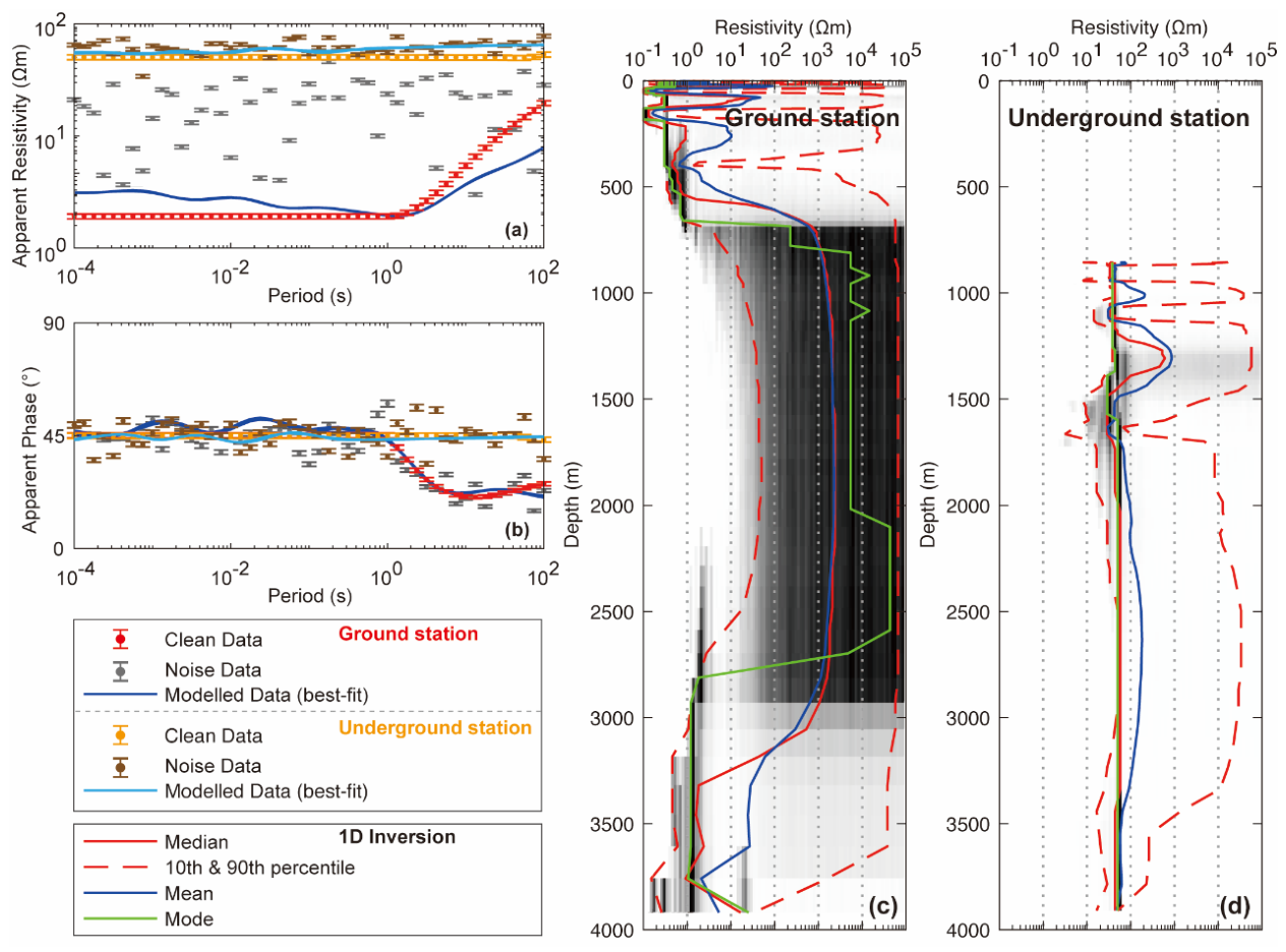
Figure 5.
Apparent resistivity and phase curves of the Huainan surface station (elevation: +22 m; a) and underground station (elevation: −848 m; b). “+” and “*” denote the XY- and YX-mode data, respectively.
Figure 5.
Apparent resistivity and phase curves of the Huainan surface station (elevation: +22 m; a) and underground station (elevation: −848 m; b). “+” and “*” denote the XY- and YX-mode data, respectively.
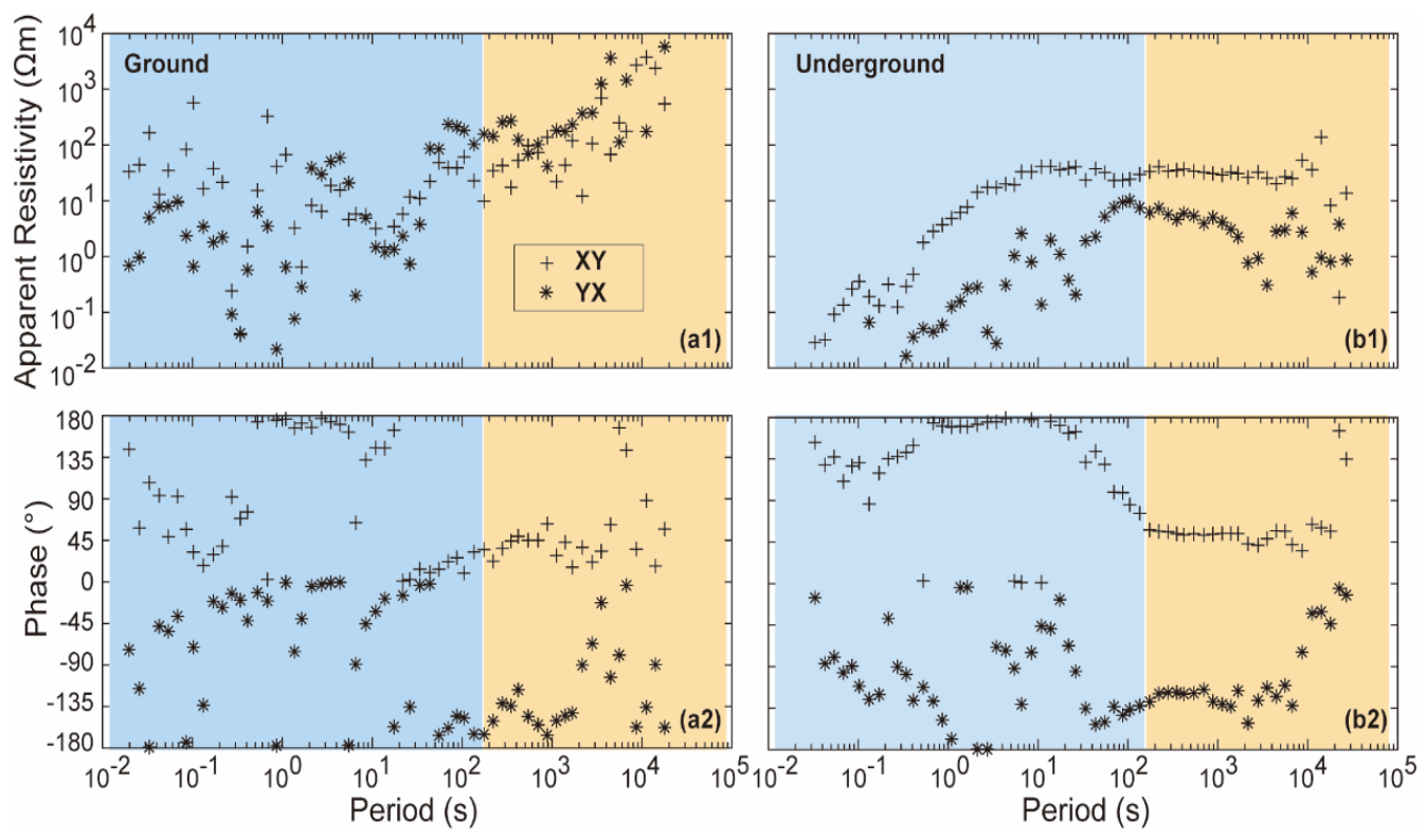
Figure 6.
1D inversion results for the field-observed surface station (elevation: +22 m) and underground station (elevation: −848 m). (a) Apparent resistivity curves; (b) phase curves. Gray dots and solid lines represent the surface data and corresponding inversion fits, respectively. Orange dots and solid lines represent the underground data and corresponding inversion fits, respectively. Red dots and solid lines represent the underground data in the low frequency period range of 100–2000 s and the corresponding inversion fits, respectively. (c–e) Posterior probability statistics of the 1D inversion models for the surface, underground, and low frequency underground data, respectively. Red solid line: median model; red dashed lines: 10th and 90th percentile models; blue solid line: mean model; green solid line: mode model.
Figure 6.
1D inversion results for the field-observed surface station (elevation: +22 m) and underground station (elevation: −848 m). (a) Apparent resistivity curves; (b) phase curves. Gray dots and solid lines represent the surface data and corresponding inversion fits, respectively. Orange dots and solid lines represent the underground data and corresponding inversion fits, respectively. Red dots and solid lines represent the underground data in the low frequency period range of 100–2000 s and the corresponding inversion fits, respectively. (c–e) Posterior probability statistics of the 1D inversion models for the surface, underground, and low frequency underground data, respectively. Red solid line: median model; red dashed lines: 10th and 90th percentile models; blue solid line: mean model; green solid line: mode model.
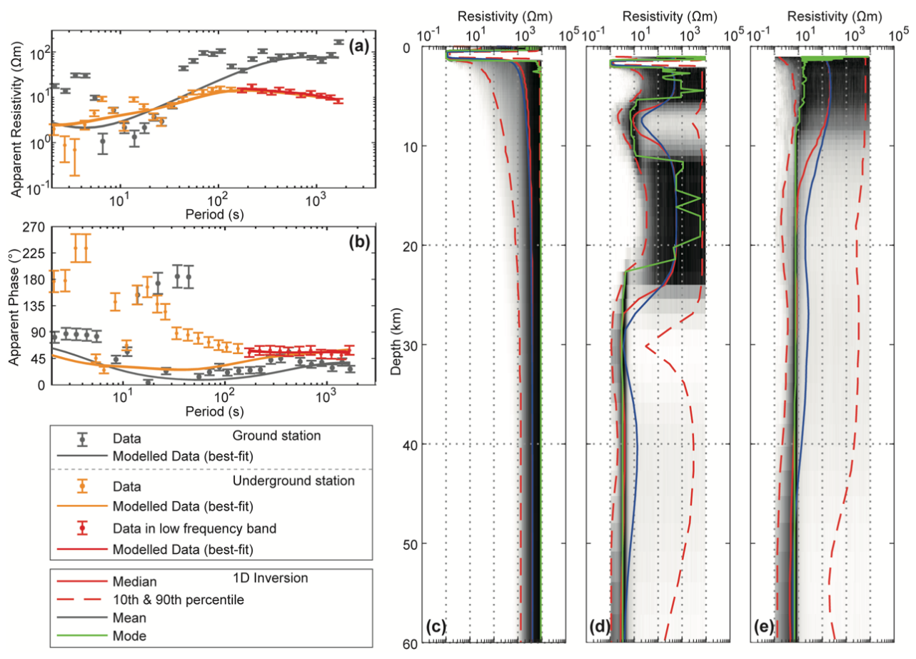
Figure 7.
Illustration of the synthetic 3D resistivity model. The shallow sedimentary layer has a resistivity of and thickness of h₁ = 870 m and/or 5000 m. The host rock has a resistivity of . The gray cuboid represents a 3D high resistivity body with dimensions of 30 km 30 km 20 km (length width height). The anomaly is buried at a depth of 30 km, and the distance from its center to the lateral boundaries of the model domain is 35 km. The anomaly resistivity was set to 55, 60, 100, and 1000 Ω·m. An MT profile was deployed at the surface, crossing the center of the anomaly. The black filled triangle marks the surface projection of the anomaly center.
Figure 7.
Illustration of the synthetic 3D resistivity model. The shallow sedimentary layer has a resistivity of and thickness of h₁ = 870 m and/or 5000 m. The host rock has a resistivity of . The gray cuboid represents a 3D high resistivity body with dimensions of 30 km 30 km 20 km (length width height). The anomaly is buried at a depth of 30 km, and the distance from its center to the lateral boundaries of the model domain is 35 km. The anomaly resistivity was set to 55, 60, 100, and 1000 Ω·m. An MT profile was deployed at the surface, crossing the center of the anomaly. The black filled triangle marks the surface projection of the anomaly center.
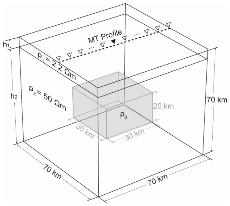
Figure 8.
Surface electric-field response of a buried 3D resistivity anomaly beneath a conductive sedimentary layer. The horizontal axis represents the distance along the MT profile, with 0 km indicating the center of the anomaly. The vertical axis represents the amplitude difference between the responses of the resistivity-anomaly models and that of a 50 Ω·m homogeneous medium (). The sedimentary layer thicknesses are 5000 m (solid lines) and 870 m (dashed lines). The anomaly resistivities are 55 Ω·m (black lines), 60 Ω·m (blue lines), 100 Ω·m (orange lines), and 1000 Ω·m (red lines). Panels (a–e) show the response curves at periods of 10,000, 1000, 100, 10, and 1 s, respectively.
Figure 8.
Surface electric-field response of a buried 3D resistivity anomaly beneath a conductive sedimentary layer. The horizontal axis represents the distance along the MT profile, with 0 km indicating the center of the anomaly. The vertical axis represents the amplitude difference between the responses of the resistivity-anomaly models and that of a 50 Ω·m homogeneous medium (). The sedimentary layer thicknesses are 5000 m (solid lines) and 870 m (dashed lines). The anomaly resistivities are 55 Ω·m (black lines), 60 Ω·m (blue lines), 100 Ω·m (orange lines), and 1000 Ω·m (red lines). Panels (a–e) show the response curves at periods of 10,000, 1000, 100, 10, and 1 s, respectively.
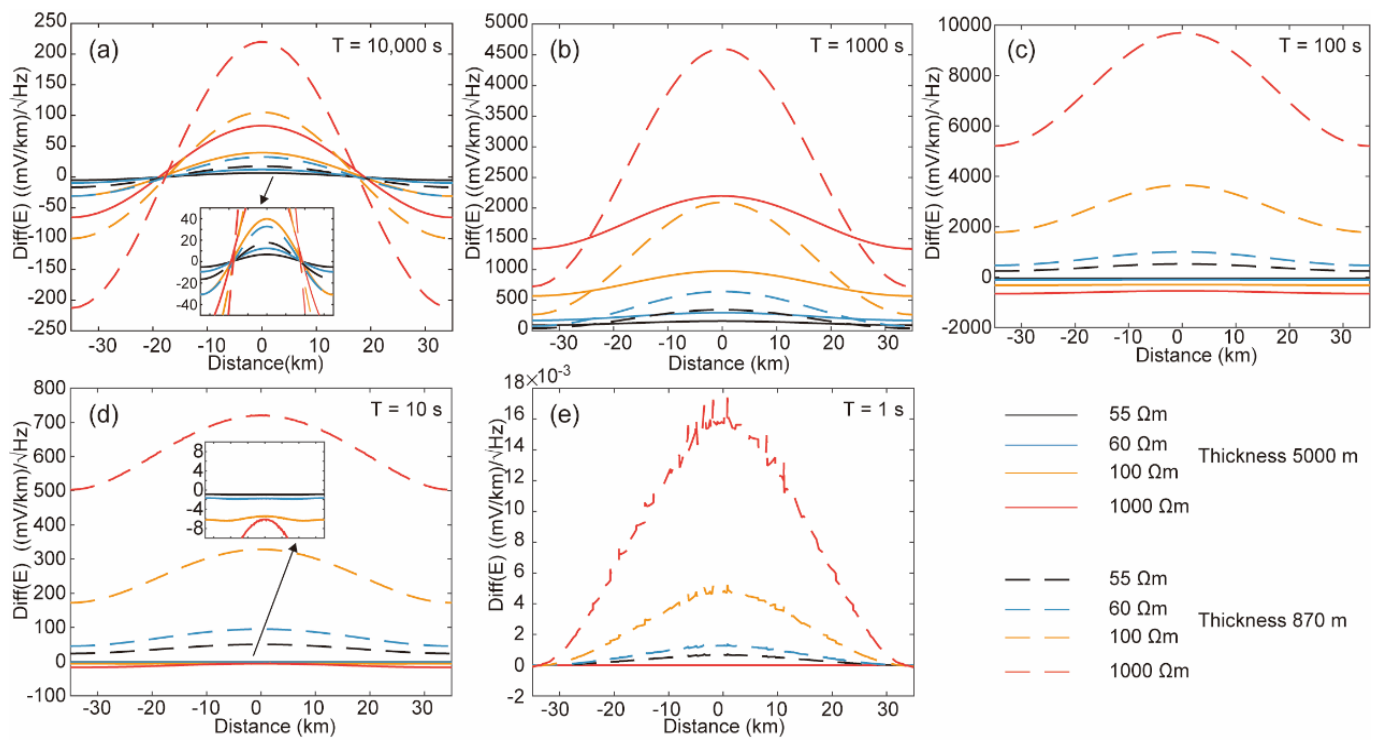
Figure 9.
Surface magnetic-field response of a buried 3D resistivity anomaly beneath a conductive sedimentary layer. The horizontal axis represents the distance along the MT profile, with 0 km indicating the center of the anomaly. The vertical axis represents the amplitude difference between the response of a 50 Ω·m homogeneous medium and those of the resistivity-anomaly models (). The sedimentary layer thicknesses are 5000 m (solid lines) and 870 m (dashed lines). The anomaly resistivities are 55 Ω·m (black lines), 60 Ω·m (blue lines), 100 Ω·m (orange lines), and 1000 Ω·m (red lines). Panels (a–e) show the response curves at periods of 10,000, 1000, 100, 10, and 1 s, respectively.
Figure 9.
Surface magnetic-field response of a buried 3D resistivity anomaly beneath a conductive sedimentary layer. The horizontal axis represents the distance along the MT profile, with 0 km indicating the center of the anomaly. The vertical axis represents the amplitude difference between the response of a 50 Ω·m homogeneous medium and those of the resistivity-anomaly models (). The sedimentary layer thicknesses are 5000 m (solid lines) and 870 m (dashed lines). The anomaly resistivities are 55 Ω·m (black lines), 60 Ω·m (blue lines), 100 Ω·m (orange lines), and 1000 Ω·m (red lines). Panels (a–e) show the response curves at periods of 10,000, 1000, 100, 10, and 1 s, respectively.
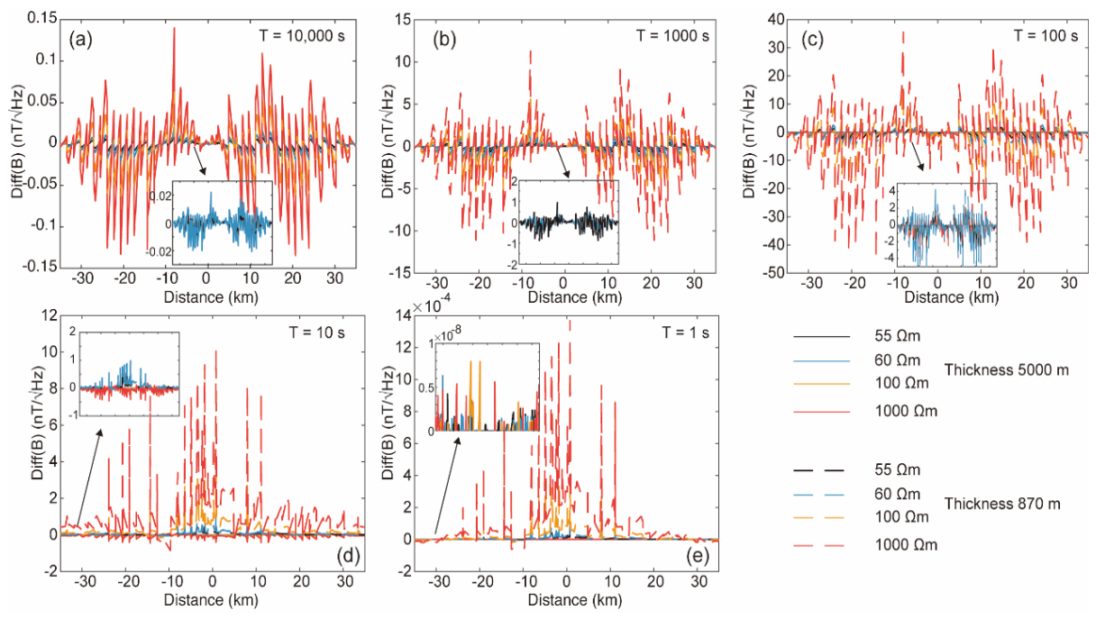
Figure 10.
Apparent resistivity response of a buried 3D resistivity anomaly beneath a conductive sedimentary layer. The horizontal axis represents the distance along the MT profile, with 0 km indicating the center of the anomaly. The vertical axis represents the apparent resistivity difference between the responses of the resistivity-anomaly models and that of a 50 Ω·m homogeneous medium (). The sedimentary layer thicknesses are 5000 m (solid lines) and 870 m (dashed lines). The anomaly resistivities are 55 Ω·m (black lines), 60 Ω·m (blue lines), 100 Ω·m (orange lines), and 1000 Ω·m (red lines). Panels (a–e) show the response curves at periods of 10,000, 1000, 100, 10, and 1 s, respectively.
Figure 10.
Apparent resistivity response of a buried 3D resistivity anomaly beneath a conductive sedimentary layer. The horizontal axis represents the distance along the MT profile, with 0 km indicating the center of the anomaly. The vertical axis represents the apparent resistivity difference between the responses of the resistivity-anomaly models and that of a 50 Ω·m homogeneous medium (). The sedimentary layer thicknesses are 5000 m (solid lines) and 870 m (dashed lines). The anomaly resistivities are 55 Ω·m (black lines), 60 Ω·m (blue lines), 100 Ω·m (orange lines), and 1000 Ω·m (red lines). Panels (a–e) show the response curves at periods of 10,000, 1000, 100, 10, and 1 s, respectively.
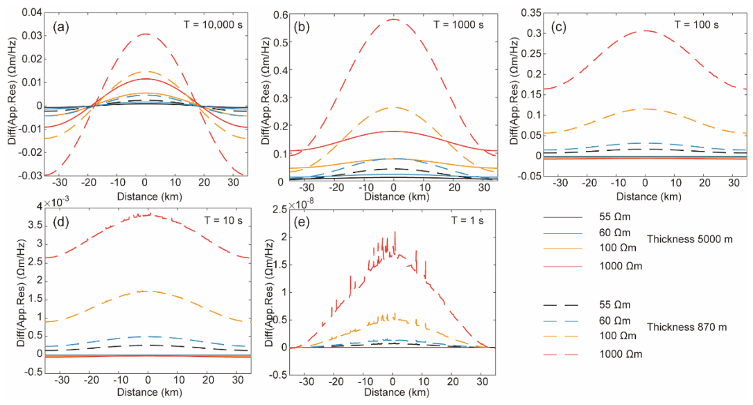
Figure 11.
Comparison of frequency-dependent MT responses at surface and underground stations. The model is shown in Figure 7, with a sedimentary layer thickness of 5000 m. The stations are located at the surface (0 m, black lines), at −870 m (blue lines), and at −5000 m (orange lines), corresponding to the vertical projection of the anomaly center at each depth. The resistivity of the 3D resistive body is set to 60 Ω·m (solid lines) or 1000 Ω·m (long-dashed lines), whereas the short-dashed lines represent the differences between the two cases (, where denotes the electric field, magnetic flux density, or apparent resistivity, respectively). (a) Electric-field response. (b) Magnetic-field response. (c) Apparent resistivity response. The gray-shaded areas indicate high frequency distortion bands caused by the mismatch between mesh resolution and frequency.
Figure 11.
Comparison of frequency-dependent MT responses at surface and underground stations. The model is shown in Figure 7, with a sedimentary layer thickness of 5000 m. The stations are located at the surface (0 m, black lines), at −870 m (blue lines), and at −5000 m (orange lines), corresponding to the vertical projection of the anomaly center at each depth. The resistivity of the 3D resistive body is set to 60 Ω·m (solid lines) or 1000 Ω·m (long-dashed lines), whereas the short-dashed lines represent the differences between the two cases (, where denotes the electric field, magnetic flux density, or apparent resistivity, respectively). (a) Electric-field response. (b) Magnetic-field response. (c) Apparent resistivity response. The gray-shaded areas indicate high frequency distortion bands caused by the mismatch between mesh resolution and frequency.
Disclaimer/Publisher’s Note: The statements, opinions and data contained in all publications are solely those of the individual author(s) and contributor(s) and not of MDPI and/or the editor(s). MDPI and/or the editor(s) disclaim responsibility for any injury to people or property resulting from any ideas, methods, instructions or products referred to in the content. |
© 2026 by the authors. Licensee MDPI, Basel, Switzerland. This article is an open access article distributed under the terms and conditions of the Creative Commons Attribution (CC BY) license (http://creativecommons.org/licenses/by/4.0/).
Copyright: This open access article is published under a Creative Commons CC BY 4.0 license, which permit the free download, distribution, and reuse, provided that the author and preprint are cited in any reuse.