
Submitted:
20 July 2026
Posted:
21 July 2026
You are already at the latest version
Abstract
This study proposes a new method for the topological synthesis of principal component projections and hydrogeochemical stoichiometric equality lines on self-organizing map (SOM) component planes to assess groundwater chemistry forming factors and quality in the Pleistocene unconfined aquifer of the Southern Bug and Sinyukha interfluve area, Ukraine. The hydrogeochemical characteristics clustered by the SOM were further examined using the graphical cross-validation method. The groundwater dataset used in the analysis consisted of 10 parameters (i.e., pH, total dissolved solids, Ca2+, Mg2+, Na+, K+, HCO3-, Cl-, SO42-, and NO3- ) from 91 samples collected during the dry season. Subsequently, for SOM construction, we utilized six log-ratio relationships of milliequivalent ion concentrations. Based on the results, the hydrogeochemical groundwater data were classified into three clusters, which revealed three water types and processes controlling their chemistry: salinity driven by sulphate inputs (Cluster 1), highly salinity driven by nitrate-chloride and sulfate pollution (Cluster 2), and relatively fresh water governed by natural carbonate dissolution and silicate weathering (Cluster 3). The salinity types were identifiable in the northern part of the study area, characterized as the primary zone of initial intense pollution. High salinity types were identified in the eastern and south-eastern parts of the territory (with delayed water exchange), whereas relatively fresh types were identified in the central part (with active water exchange) as well as in the western and south-western parts. Modeling confirmed that extensive sulfate, nitrate, and chloride contamination led to anthropogenic degradation of the aquifer system.
Keywords:
water-rock interaction
; log-ratio MinMax transformation
; phase transitions
; self-organizing map
; machine learning
1. Introduction
The groundwater analyzed in this study is the result of a complex interaction of natural and anthropogenic factors and is widely used by the local population for domestic, agricultural, and industrial use. The study area is 150 km2 and was declared an environmental emergency zone in August 2000 owing to increasing groundwater contamination and deteriorating health conditions in some communities. Therefore, our research prioritizes the examination of the factors controlling the chemical composition of groundwater in the Southern Bug and Sinyukha interfluves area (Ukraine). The factors governing the groundwater chemistry of natural water has been focus of many studies [1,2,3,4], with their number having increased considerably in last two–three decades [5,6,7,8,9,10,11,12,13,14]. Many of them involve graphical methods, such as the Piper diagram, Gibbs diagram, ion ratio analysis, and rock weathering plots, as well as statistical techniques, such as principal component analysis (PCA) and cluster analysis. When combined, these methods help evaluate the quality of groundwater and determine the geological and anthropogenic impacts on its chemical composition, including weathering and dissolution of minerals, evaporation, atmospheric precipitation, ion exchange and pollution [12]. In recent years, the utilization of machine learning and artificial intelligence methods for groundwater quality analysis has gained popularity [7,9,13,14,15,16,17,18,19]. Such methods may involve cluster analysis to identify representative clusters (also known as water types or hydrogeochemical facies) reflecting the processes generating natural variability in hydrogeochemical parameters. These representative clusters, which help identify key chemical trends, can provide insight into the heterogeneity and connectivity of aquifers, as well as the physical and chemical processes that control water chemistry. Specifically, Nguyen et al. [7] applied the self-organizing map (SOM) framework for the first time to decipher complex seasonal and spatial hydrogeochemical characteristics within confined aquifers. By coupling SOM clustering with classical Gibbs diagrams, they successfully identified how recharging factors shift water types from dry to rainy seasons, and distinguished between rock weathering, evaporation, and marine intrusion processes. Using the SOM framework, Nakagawa et al. [9] classified groundwater hydrogeochemical data into eight clusters, identifying three main water types based on salinity: high salinity, low salinity, and freshwater. Liu et al. [16] demonstrated the effectiveness of integrating SOMs and multivariate statistics for elucidating the complex interaction between natural hydrogeological processes and human activities affecting groundwater geochemistry in an urban environment. However, most studies utilize raw ion concentrations, pH, and total dissolved solid (TDS) as isolated parameters within the SOM framework, which does not allow for the explicit identification of dominant geochemical processes. To address this limitation, the input parameters in our study are ion combinations rather than individual concentrations, allowing the neural network to operate with process indicators rather than simple concentrations. Moreover, the proposed method, based on the projection of stoichiometric equality lines and the principal component vectors across SOM component planes, allows for the identification of dominant (competing) processes in a single format, while simultaneously revealing the underlying interrelationships. Furthermore, unlike other methods, our method, which combines log-ratio analysis, PCA, SOM, and graphical cross-validation (GCV), focuses on identifying physical stoichiometric equality isolines as well as main component isolines, converting the algorithmic “black box” into a transparent model for expert analysis. For example, the application of Support Vector Machines (SVM; [20]) via kernel functions (the “Kernel Trick”), according to [21], maps data into infinite-dimensional feature spaces to identify an optimal separating hyperplane. However, as noted in works on Interpretable Machine Learning (XAI) (e.g., [22]), such transformations render the visual tracking of physical thresholds impossible, effectively turning the process into a “black box”. The primary advantage lies in the ability to delineate cluster boundaries—uniquely facilitated by the intersection points of stoichiometric equilibrium lines and principal component vectors projected directly onto the component planes—while simultaneously distinguishing between anthropogenic and natural factors driving groundwater chemistry. Furthermore, for an independent verification of the topological conclusions and a robust assessment of hydrogeochemical process intensities, we incorporated GCV plots into our model and constructed distribution profiles of normalized balances (fi). Available hydrogeochemical research on the groundwater in the studied Pleistocene aquifer has primarily examined the chemistry of major ions, the steady-state flow, and the ecological–hydrogeological state of the groundwater [23,24]. In our previous study [25,26] we revealed the processes and factors controlling the chemical evolution of groundwater in modern and Pleistocene deposits in the Southern Bug Sinyukha interfluve area. This study investigates the role, dynamics, and interaction of these factors as well as their impact on TDS and pH. The studied unconfined aquifer, owing to its proximity to the surface and location in low-lying, topographically depressed areas, is one of the causes of groundwater pollution. Furthermore, groundwater functions as a protective barrier and source of pollution for the fissure waters of the underlying Precambrian crystalline aquifer, which is used for supplying drinking water. In this context, comprehensively examining the chemical composition of groundwater and the factors controlling its formation is a priority for the study area and wider region. The objective of this study was to cluster groundwater chemistry controlling factors and investigate their impact on groundwater quality in the unconfined aquifer in the Southern Bug and Sinyukha interfluve area using log-ratio analysis, PCA, SOM, and GCV. This study's findings will yield significant insights into the spatial hydrogeochemical properties of groundwater within the Pleistocene unconfined aquifer of the study area. Furthermore, the proposed method outperforms standard “black box” solutions in interpretability and provides a robust framework for verifying the boundaries of hydrogeochemical data clusters, which will be essential for accurately evaluating the quality and spatiotemporal evolution of groundwater chemical composition across the region.
2. Materials and Methods
2.1. Study Area
The study area is in the southern part of the Ukrainian reservoir of strata-fissure waters on the territory of the Southern Bug and Sinyukha interfluves (Figure 1). This area is a typical agricultural and industrial area, located in the steppe zone of southern Ukraine, and belongs to the arid zone of insufficient moisture. Here, the dry season sets in during the second half of June and the first half of November, with precipitation decreasing, and evaporation reaching peak values.
The study area is characterized by gently rolling plains dissected by river valleys and gullies, with the slopes being eroded by gullies and ravines. Absolute relief marks range from 130 to 247 m. The lithologic–stratigraphic complex of the Pleistocene and Holocene includes the following [24]: an aquifer in the alluvial, proluvial–deluvial sediments of the river floodplains and the gully bottoms; and a locally weak aquifer in the aeolian–deluvial deposits of the watershed plateau (Figure 1). The lithology of the Pleistocene aquifer comprises mainly sand, sandy loam, loam sometimes with carbonate, and clay with gypsum crystals and silt sometimes with crystalline rocks. These sediments comprise mainly quartz, calcite, dolomite, gypsum, and feldspar. Weathering and dissolution of these minerals is a possible source of groundwater enrichment with different ions. The depth of the groundwater level varies from 0.0–5.0 to 10.0–15.0 m. The thickness of the water-filled layer is 0.5–3.0 m—sometimes up to 5.0 m. Groundwater recharge is facilitated by atmospheric precipitation, surface water, and inflow of pressure water from the crystalline base through decompaction zones. During low-water periods, discharge occurs into rivers and underlying aquifers—provided there is no low-permeability rock present. The groundwater is widely used by the local population in numerous boreholes for domestic and agricultural purposes. In this area there are about 35 anthropogenic sources of groundwater pollution such as industrial and domestic landfills, pesticide and fertilizer storage, various livestock farm complexes, settling tanks, wastewater and solid waste discharges, and so on. These anthropogenic items have an impact on the geological environment—especially concerning its hydrosphere. Incisions, such as river valleys and ravines, which host populated regions and their agricultural complexes, are particularly prone to technogenic influences. In addition, groundwater serves as a protective screen and source of contamination for the underlying Precambrian Crystalline Aquifer, which is used for supplying drinking water. These aquifers are hydraulically connected mainly in gullies or river valleys.
2.2. Sample Collection and Analysis
Groundwater samples were processed for a short chemical analysis, estimating the content of nitrogen group compounds and spectral analysis of the dry residue [24]. Sampling was performed at eight monitoring wells and 25 dug wells, which are located in the territory of Boleslavchik Village. Monitoring wells were drilled along the slope of the central part of the village (north–south profile; profile line P-1–P-6 in Figure 1) and along the bottom of the gully (east–west profile; profile line P-7–P-8 in Figure 1). Sampling was conducted during the late-summer low-flow stage (specifically from August 30 to September 21, 2000) in accordance with the guidance for sampling, preservation and processing of groundwater samples recommended by the State Agency for Water Resources of the Ministry of Environmental Protection and Natural Resources of Ukraine. Chemical analyses were performed by the accredited Research Central Laboratory of the Black Sea Coastal Regional Geological Enterprise “Prichomomor DRGP” (Odessa, Ukraine), following the standard examination methods for drinking water quality assessment (aligned with DSanPiN 2.2.4-171, [27]). Temperature and pH were measured at the sampling site to account for possible physicochemical changes. All samples were filtered through a 0.45-μm membrane filter and collected in clean, dry plastic bottles made of polyethylene or high-density polytetrafluoroethylene.
2.3. Data Used and Pre-Processing
Primary data used in our study comprised 91 groundwater samples with 10 parameters including pH, TDS and major ions (, , , , , , , and ). In terms of the charge balance error (CBE), groundwater quality was satisfactory (CBE < ±2.5%). The average chemical composition of groundwater is listed in Table 1. According to Piper diagrams in our previous study, the dominant hydrochemical types of the studied shallow groundwater are sodium bicarbonate, sodium sulfate and sulfate–magnesium–sodium, sulfate–calcium–sodium types, and sometimes nitrate–hydrocarbonate and nitrate–chloride–sodium types [26,27].
Building upon our previous work defining hydrogeochemical facies [26,27], this study employs a modified approach combining log-ratio analysis, PCA, SOM, and GCV to analyze the evolution of the dynamic system. For the application of SOM, we adopted six dimensionless parameters—i.e., f1 – f5 (Table 2, column 2) and ln(pH). Parameters f1 – f5 can be interpreted as factor or criteria of hydrogeochemical dynamic similarity. Previously, we identified these factors using graphical methods [1,4,12,28], including Gibbs diagrams, as well as binary plots of the major ions [25]. In this study, these factors were used as input parameters for the neural network. The concentrations of all ions for the factors are expressed in milliequivalents per litter (meq/L, Table 2). To satisfy multivariate normality and reduce outlier effects [29,30,31], a log-transformation was applied to both the parameters f1 – f5 and pH. Column 5 in Table 2 is the result of a generalization of numerous scientific results [1,4,12,26,28].
Importantly, to ensure conceptual clarity, the specific values on the SOM feature maps (e.g., 0.31 for f1 and 0.14 for f3 in Table 2) are defined as normalized stoichiometric 1:1 thresholds (Thnorm). These values do not represent classic hydrogeochemical characteristics for mineral equilibrium derived from laboratory experiments. Instead, each Thnorm represents dataset-specific topological projection of the physical 1:1 ionic equivalence line (ln(Y/X) = ln(1) = 0)). The spatial representation of this 1:1 boundary on the SOM is defined as the stoichiometric equality line. Since each log-ratio parameter has its own unique empirical minimum and maximum range, the physical zero maps onto a different normalized value for each individual feature. Following log-ratio pre-processing, each fi was treated by PCA and SOM as an independent feature. Min–Max scaling was used to preserve the original data distribution shape and correlation structures within the feature space F. Many researchers apply isometric (ILR) or centered (CLR) log-ratio transformations to classify water types based on percentage compositions [32,33]; however, in this study, we did not adopt these approaches. Since our data represent arbitrary geochemical intensity indicators rather than parts-of-a-whole (proportions), CLR or ILR would be counterproductive, confounding specific thresholds (e.g., fi =0 for stoichiometric equality) with the variance of other features. In our approach, the logarithmic space ensures a unique global equilibrium at fk = ln(1) = 0, preserving the physical interpretability of SOM isolines to distinguish competing processes. Furthermore, the model is robust against translation or scaling, while shifting the normalized stoichiometric 1:1 threshold does not distort the data. Consequently, multiplicative relationships can be transformed into additive ones.
2.4. Efficiency of SOMs for Hydrogeochemical Data Analysis: Configuration and Training
The SOM framework, developed by Kohonen [34,35], is a type of artificial neural network trained through unsupervised learning. The SOM algorithm projects high-dimensional data into a low-dimensional latent space, creating a regularized map based on data similarity and competitive neural principles. Unlike traditional deterministic models, the SOM framework preserves the inherent universality and nonlinear complexity of relationships between hydrogeochemical characteristics. Geological similarity is predominantly approximate, as most geological processes are multifactorial and operate across vast spatiotemporal scales. The dual nature of geological formations—i.e., “locally heterogeneous, yet globally homogeneous”—requires a tool capable of capturing generalized features (the “homogeneous in total”), while accommodating local variances. In this study, the SOM provides a synergistic effect, integrating input parameters into a unified topological structure that mirrors the evolutionary complexity of groundwater composition. Furthermore, the topological consistency of the SOM allows for the overlay of theoretical stoichiometric equality lines and PC projections, transforming the visual map into a robust tool for identifying phase transitions, hydrogeochemical bifurcation points, and so on. The SOM is a robust tool for clustering and data mining facilitating the extraction of essential information in hydrogeochemistry [7,9,10,13,14,15,16,18,30,36,37,38,39,40]; it maps high-dimensional input space onto reference (weight) vectors through three stages: node competition, winning node selection (best-matching unit), and weight updating via Euclidean distance [41]. Designing an appropriate SOM structure—specifically the number of nodes (m) and the grid’s aspect ratio—is crucial [42]. In this study, the total number of nodes was determined using the heuristic rule—i.e., where n is the number of samples. The grid’s side lengths were set according to the square root of the ratio between the two largest eigenvalues () derived from PCA [36,43]. All log-ratio data were normalized using Min–Max scaling to a range of [0, 1]. Given the limited dataset (n=91), linear initialization was preferred [30,41]. Training was performed in batch mode for 6000 iterations using a Gaussian neighborhood function. The initial learning rate and neighborhood radius were 0.37 and 2.40, respectively. Map accuracy was evaluated through the quantization error (QE) and topographic error (TE) [35]. For 91 groundwater samples, the optimal map size was calculated as 8×6 (48 nodes). The resulting QE and TE values were 0.13 and 0.00, respectively. Adjacent node distances were visualized using a U-matrix.
2.5. Multivariate Statistical and Graphical Methods. Topological Invariance Analysis
Hierarchical Cluster Analysis (HCA), using Euclidean distance and Ward’s linkage, grouped six hydrogeochemical parameters (Table 2). The optimal cluster count, determined by a dendrogram phenon line, was validated using the Silhouette coefficient [44,45]. PCA revealed the dataset’s latent structure via orthogonal variables [43]. In this study, a key methodological innovation is the integration of the Thnorm line and PC1 and PC2 projections into the SOM structure. Thnorm acts as a topological boundary distinguishing process dominance (fi > Thnorm or fi < Thnorm). Owing to log-ratio transformation and Min–Max scaling, the SOM topology remains invariant to scalar multipliers of initial concentrations. This allows dynamic rethinking of process dominance zones—by shifting the stoichiometric threshold Thnorm—without recalculating the model. To verify these conclusions, GCV analysis and normalized Δfi balance profiles were constructed against TDS and pH, with the line ln(Y/X) = 0 becoming the universal axis of stoichiometric equality (Thnorm), dividing the zones of unconditional dominance (> 0 for Yi; <0 for Xi), and enabling the evaluation of parameter dynamics within SOM planes. HCA and PCA were performed using a modified SciPy package (https://scipy.org/, accessed on September 2024) in Python environment.
2.6. Topological Synthesis of PCA Projections and Hydrogeochemical Stoichiometric Equality Lines on the SOM Surface. Nonlinear Projection of Balance Relations
We define the feature space as a set of N logarithmic parameters (in this study, N = 6): , where each feature fk is calculated as the logarithm of the ratio of a pair of initial concentrations of hydrogeochemical elements Yi, Xj (measured in meq/L) or as the logarithm of the hydrogen exponent (pH):
where i, j ∈ {1,…, n}, and n is the number of initial components in the system. Despite fk being derivative functions, they are treated by the mathematical models (i.e., SOM and PCA) as statistically independent coordinates of the input vector. In additive balance space, the value fk = 0 strictly corresponds to the point of physical equilibrium (Yi = Xj), justifying the application of the Euclidean metric in the SOM and PCA algorithms for the objective assessment of process dominance. Each feature fk was transformed into a dimensionless value within the range of [0, 1] according to the following expression:
where fk,min and fk,max are the minimum and maximum values of the feature fk across the entire dataset, respectively. The SOM is defined as a nonlinear mapping Φ from the high-dimensional space of normalized features onto a discrete two-dimensional lattice of neurons M (latent space) [35,46]:
where wp is the weight vector of neuron p (p = 1,…, m), and m is the total number of neurons. The Thnorm on the component plane for feature fk is defined as the set of neurons where the weights satisfy the condition of physical equality between components (Yi =Xj):
The threshold value sk in the normalized space is calculated as follows:
where 0 corresponds to the value of ln(Yi /Xj) at equilibrium, and fk,min and fk,max are the extrema of the initial log-ratio feature fk. The principal component projections onto the SOM surface are calculated as the dot product of the neuron weight vectors and the PCA loading vectors:
where ξ1 and ξ2 is the first and second eigenvectors (loadings) of the covariance matrix of the normalized data, and N is the number of features. For GCV analysis, the transition to logarithmic relations in normalized space is conducted as follows:
Eventually, the SOM map is segmented into physically distinct operational regimes: domains Ω1 and Ω2, representing the dominance of competing hydrogeochemical processes. The modified software MiniSom (https://pypi.org/project/MiniSom/, accessed on September 2024) was utilized for constructing the SOM model.
fk = ln(Yi /Xj) or fk = ln(pH),
3. Results and Discussion
3.1. SOM and Clustering Results: SOM-Based Visualization of Multivariate Data
The component planes for the 48 reference vectors (nodes) of the six log-ratio parameters (f1, f2, f3, f4, f5, and pH), normalized to a range of [0, 1], are presented in Figure 2. HCA was applied to the SOM prototypes using Ward’s linkage algorithm and the Euclidean distance measure. The first principal component accounts for 42.6% of the total variance, largely driven by feature f3 (loading value of 0.82). The second principal component accounts for 34.4% of the total variance, with f5 being the parameter most closely associated (loading value of 0.80). The optimal number of clusters (three) was determined by maximizing the silhouette coefficient (Figure 3a), which reached its peak score of 0.40 with three clusters. This optimal partitioning is visually confirmed by the phenon line in the dendrogram (Figure 3c), drawn at a linkage distance of 17. The resulting low QE of 0.14 and perfect TE of 0.00 further indicate optimal model training and high mapping quality. The orange isoline on the component planes indicates the projection of the hydrogeochemical stoichiometric equality line (Thnorm). The threshold values (sk) for Thnorm for each SOM plane were calculated according to Equation (5). The green solid isolines represent multiples of the sk threshold. The red and blue dotted lines represent the projections of PC1 and PC2 onto the SOM plane, calculated using Equations (6) and (7), respectively.
The U-matrix (Figure 2g) visually confirms high distances between the three identified clusters, which delineate physically distinct hydrogeochemical facies. The coincidence of Thnorm isolines with zones of high inter-neuron distance on the U-Matrix proves that the equilibrium line acts as a natural topological barrier. A preliminary visual qualitative analysis of the component SOM maps (Figure 2) and clustering results reveals the specific characteristics of each cluster. For example, Cluster 1 (left of Figure 2h) is associated with high values of f1, f2, f3 and f5, primarily observed in the upper-left regions of the respective component planes (Figure 2a–c, 2e). Cluster 2 is characterized by high values of f1, f3, and f4 (the zones below Thnorm), relatively high values of f5 (lower part of Cluster 2), and high values of pH (hexagon almost in the center of the pH SOM), with low values being concentrated in the right corner. Cluster 3 is characterized by high values of f2, f4 (the zones below Thnorm), and f5 and relatively high values of f1 (to the right of the Thnorm). Also highlighted here are the low pH values for a small number of samples in the lower right corner of the SOM map (Figure 2f). Since SOM clusters data based on the similarity measure of multidimensional feature vectors, the clustering of factors (features f1– f5) in this study can also be interpreted as a clustering of hydrogeochemical dynamic similarity criteria.
3.2. SOM and Clustering Results: Topological Discontinuity and Singularity Analysis
This section synthesizes system-scale analysis (PC1/PC2 projections) and local hydrogeochemical constraints (Thnorm) to implement phase boundary mapping. The Thnorm isolines on the SOM plane visualize objective hydrogeochemical boundaries dictated by shallow groundwater dynamics, where comparing these lines with PC vectors differentiates between equilibrium processes and external or anthropogenic drivers. Since SOM weights are normalized within the range of [0, 1], Thnorm acts as a fundamental topological boundary dividing the map into two phase zones (Table 2; Figure 2). The dominance of the process is characterized by the zone occupying a larger map area where weight vectors wp,k exceed the specific threshold sk of the specific feature. Equal zone areas signify process equivalence, and the shift of the Thnorm line on the SOM plane is mathematically equivalent to rotating the equilibrium ray in the original Cartesian coordinate system. The topological discontinuity in the PC1 projection represents a first-order mathematical singularity, corresponding to a sharp or inverse gradient in weight vectors where smooth evolutionary trajectories are interrupted by a hydrogeochemical barrier. Its physical nature as a genuine hydrogeochemical barrier—rather than a multidimensional projection artifact—is confirmed by contour crowding (Figure 2a and Figure 2c) and topological loops or intersections (Figure 2b, Figure 2d, Figure 2e). Contour crowding before the discontinuity and abrupt value changes indicate a sharp barrier, typically representing water mixing, phase transitions (e.g., rapid pH shifts), or intense anthropogenic pressure (point-source pollution or localized over-pumping). This is confirmed by Figure 2e and Figure 2f, where neurons containing samples 57, 72 and 75 show a sharp jump in pH, making linear interpolation of isolines impossible. The area between PC1 discontinuities represents a maximum entropy zone where dissolution forces and anthropogenic pressures counteract, creating inverted U-shape patterns (Figure 2a). According to [47,48], this inverse U-shaped pattern of PC1 and isolines that are proportional to Thnorm indicates a topographic break in a nonlinear data manifold, which is not a dimensionality artifact [49]. In a hydrogeochemical context, it confirms a sharp phase transition where the primary vector (PC1) fails to continuously approximate the process, visualized as a first-order discontinuity. For instance, limit analysis (one-sided limits) in Figure 2a reveals a functional jump typical of physical–chemical barriers: Values increase on the left side of the break (0.50, 0.60, 0.70, 0.75, and 0.80), whereas the right side begins at a different order (0.70, 0.75, and 0.80). Furthermore, the PC1 isoline runs parallel to Thnorm, defining the first cluster boundary and proving it is a determinant for PC1. Thus, PC1 isoline segmentation demonstrates system nonlinearity and stepwise hydrogeochemical evolution through critical barriers. Plotting the blue dashed PC2 isoline across all planes is essential to identify secondary processes masked by the dominant PC1 trend. The intersection of systemic axes (PC1, PC2) with Thnorm isolines enables a comprehensive topological model of phase transitions. In PC1 discontinuity zones, the variance of secondary factors (PC2) increases and overcomes the global trend resistance threshold, suggesting that the local physical–chemical potential of a specific feature (e.g., f5) becomes dominant at critical points. In the middle upper layer of SOM maps (Figure 2), where the left branch of PC1 and the PC2 line approach orthogonally to the boundary separating Clusters 1 and 3, PC2 intensity resists the global PC1 trend and reaches a critical level. At this junction, the global trend weakens, causing an isoline break where the secondary process (feature f5) becomes sufficient to pierce the cluster boundary, transitioning the system into a new state. The alkaline core region, where PC1 and PC2 approach the boundary of Clusters 2 and 3 (Figure 2f), locally represents a bifurcation point where the system determines its evolutionary direction. Inter-cluster boundaries (Figure 2h) are determined by the approximation of principal components and Thnorm isolines. For instance, the boundary between Clusters 1 and 2 coincides with the PC1 trajectory and the multiple stoichiometric equality isoline Thnorm = 0.5. The boundary between Clusters 2 and 3 is defined by the PC1 vector up to the third row of the neural grid (prior to the PC2 and f5 stoichiometric isoline intersection); after the intersection, it is dictated by the PC2 trajectory. Topologically, boundaries are fixed where PC1 and PC2 become collinear with stoichiometric equality isolines. Furthermore, the intersection points of isolines sk, Thnorm, and PC2 with the PC1 global trend consistently pass along the cluster boundaries, thereby playing a constructive role in the formation of cluster boundaries. Such critical threshold points are clearly visible in Figure 2b, Figure 2d and Figure 2e and on the distance matrix (U-matrix) in Figure 2g. The system includes two functional relations based on PC1 loadings. The first group includes features with significant positive loadings (e.g., f1, f3, and the more complex f5), where PC1 isolines do not intersect Thnorm as these parameters themselves dictate the PC1 trajectory. The second group consists of features with negative loadings (f2 and, f4) that oppose the global trend; their Thnorm isolines intersect the PC1 vector, creating bifurcation points and complex cluster boundaries. This interaction assesses the resistance of local geochemical balances to systemic forcing, marking structural transformation zones. Thus, this topological synthesis transforms the passive SOM visualization into a phase diagram.
3.3. Phase Boundary Mapping via ln(Yi/Xi) Topological Synthesis of Feature Balances (f1–f5)
On the f1 component plane (Figure 2a), most samples lie above the Thnorm line (sk = 0.31; Table 2), indicating dominance over driven by sulfate dissolution or cation exchange. The area below Thnorm reflects carbonate dissolution, while proximity to the line indicates mixed mineral weathering. The convex sk = 0.5 isoline (inverted U-shape) between discontinuous PC1 segments marks a phase transition from natural weathering to an anthropogenic regime. This shift features a superposition effect where sulfate dissolution increases ionic strength, triggering ion exchange, while localized pollution shifts the system from its primary PC1 trajectory, causing sharp pH fluctuations (Figure 2f). Alignment between the left PC1 branch and the sk = 0.5 isoline shows that the latter determines PC1, confirming that PC1 segmentation reflects nonlinearity and stepwise evolution across discontinuities. This topological gap represents a hydrogeochemical barrier created by mineral dissolution, ion exchange, and wastewater input, which the system overcomes in a stepwise, nonlinear manner. The biplot (Figure 3b) confirms f1 as a primary driver with the second-highest positive PC1 loading. The PC1 discontinuity signals critical instability in the growth process, where the system deviates from its trajectory, crosses an equilibrium zone, and restabilizes in Cluster 3. At the C1/C3 boundary (Figure 2f), converging PC1 and PC2 trajectories suggest a regime transition where dominance shifts to feature f5 (maximum PC2 loading). The f2 plane indicates dolomite dissolution and cation exchange beyond Thnorm lines, while the segment between sk=0.59 and sk =0.72 reflects calcite dissolution. Decreasing f2() alongside increasing f3 signals external sulfate inputs driving magnesium dominance via cation exchange. The negative PC1 loading of f2, intersecting multiple stoichiometric isolines, confirms a shift toward a magnesium-dominated regime via dedolomitization and evaporative concentration. The f3 map (Figure 2c) shows sulfate dominating over calcium, linking ion sources to sulfate mineral dissolution. High topological similarity of f1, f2, and f3 in upper-left quadrants confirms synergistic processes in Cluster 1. This phase exhibits and enrichment with calcium suppression, linked to Na+/K+ ion exchange (Figure 2d). Absent halite and marine impact involving elevated sulfate with trace elements (Cr, Li, Ni, Ti, and Zr) suggests sulfide oxidation and anthropogenic influences. Feature f3 has the maximum positive loading on PC1, driving the system’s main evolutionary vector. The alignment of PC1 parallel to isolines confirms that the system variability depends on the f3 distribution. This isoline fusion with the PC1 projection marks the cluster boundary as a phase threshold defining sulfate regime stability. Conversely, PC2 projection intersecting isolines perpendicularly in Cluster 2 indicates that the secondary factor acts as a disruptor to the equilibrium. The f4 component plane (Figure 2d) reflects sulfate and chloride dominance (likely from anthropogenic runoff and fertilizers) over silicate weathering, with . A 180° inversion between f4 and f2, relative to f1, indicates a facies shift from bicarbonate to sulfate–chloride–sodium types. Holding the second-highest negative PC2 loading, f4 regulates local salinization independently of the primary PC1 trend. The Thnorm and PC1 projection intersection in the bottom-right quadrant shows this feature’s physical threshold resists the main evolutionary vector. Isoline refraction and intersections confirm high nonlinearity within Cluster 2, matching extreme weight gradients on the U-matrix (e.g., neurons with samples 39, 73, and 89; Figs. 2g, 2h). Intersections of the PC1 and PC2 projections with the Thnorm lines on f4 and f2 maps pinpoint zones where the system balances between and and define the cluster boundaries. Finally, the Thnorm intersection with the right branch of the PC1 projection (Figure 2d), correlated with pH fluctuations (Figure 2f), marks the termination of the stable regime and a transition to a localized, different geochemical phase. The f5 component plane (Figure 2e) illustrates the synergy between anthropogenic impact and decarbonization, holding the maximum positive PC2 loading. Technogenic anions dominate over bicarbonates in 56% of samples, whereas the natural bicarbonate component prevails in the remaining 44%. An orthogonal intersection of the PC1 trajectory with Thnorm line at the boundary between Clusters 1 and 3 marks a pronounced geochemical barrier. The topological discontinuity of this line indicates a zone of intensive mixing and metamorphism where the system cannot evolve smoothly without surpassing a critical nitrate–chloride saturation threshold. Comparative analysis of the f3 and f5 planes reveals that within the phase transition zone, control is intercepted by the secondary process (PC2), making the nitrate–chloride complex the dominant factor in local variability. Consequently, feature f5 serves as a primary indicator of technogenic metamorphism, driving localized shifts in groundwater composition. The f6 (pH) component plane (Figure 2f) reveals an anomalous alkaline zone within Cluster 2, situated between discontinuous PC1 isolines. The coincidence of this node with the pH extremum identifies a critical point where anthropogenic factors intercept natural evolution. The convergence of the PC1 and PC2 trajectories above this alkaline core forms a bifurcation point, marking maximum instability where the alkaline trigger and the nitrate–chloride complex (f5) drive the topological discontinuity of the primary vector. Conversely, the lower right corner shows a localized pH decrease, signaling an acid-oxidative impulse. This acidity promotes intensive ion exchange and calcium leaching, leading to magnesium and dominance, reflected in high weights of alkali metals, magnesium, sulfate, and bicarbonate components. The localized anomaly and limited sample size in Cluster 3 confirm the technogenic origin, interpreted as point-source pollution.
3.4. Cross-Validation and Geochemical Characteristics of the Clusters
Figure 4a and Figure 4b illustrate the spatial distribution plots of hydrogeochemical features (fi), TDS, and pH relative to a unified equivalence line. To enhance the visualization of the dynamics and variability of these features, the data were categorized into two groups: f1, f2, f4 (Figure 4a) and f3, f5 (Figure 4b). Above the equivalence line, TDS dynamics are determined by technogenic factors, whereas below it, they are driven by natural processes. Features f1, f2, f3 and f5 show the highest fluctuation amplitudes, whereas f5, f2, TDS, and pH show a stable trend within Сluster 3. Positively correlated features with TDS show collinearity of isolines with respect to the PC1 vector (e.g., f1 and f3 in the border zone of Cluster 1).
Conversely, negatively correlated features show orthogonal or intersecting isolines relative to the PC1 vector, as seen for f2, f4, and f5 in Cluster 3 (neurons with samples 22 and 26), where PC1 intersects Thnorm isolines corresponding to points 23 and 27 on the GCV (Figure 4a and Figure 4b). High isoline density marks zones of intense feature growth. Parallel isolines to the PC1 vector indicate a contribution to the upward trend of TDS and pH, corresponding to progressive mineralization reaching extreme values in the spatial graphs (Figure 4a and Figure 4b, points 61, 64, 65). Conversely, orthogonal intersections of dense isolines by the PC1 vector signal a correlation inversion, exemplified by the f5 topology (Figure 2e), where the PC1 trajectory intersects Thnorm almost orthogonally, corresponding to an anticorrelation at point 51 (Figure 4b).
According to the monitoring data [23], in the study area surface water and deep groundwater exhibit only low or localized (point-source) contamination, in contrast to the shallow groundwater, which is heavily polluted. Since the study area is located within the southern part of the Ukrainian basin of stratum-fracture waters and represents a zone of intense water exchange, the pollution predominantly affected the areas with poor water exchange. This is evidenced by the elevated values of TDS and features f1, f3, and f5 observed from the north to the east and southeast in some dug wells and monitoring wells located in low water exchange conditions. The monitoring results of the study area [23] show that the soil-grounds within the vadose zone remain largely unpolluted by nitrates and are non-saline. However, the areal soil pollution by heavy metals (Ti, Cr, and Li) and point-source pollution by (Ni and, Zr) are clearly traced. This represents fingerprint of technogenic pollution, where the active phase has migrated from the ground surface into the unconfined groundwater aquifer and has been partially immobilized within the zones of poor water exchange. A joint analysis of SOM planes and GCV, while considering also Figure 1, allowed the identification of the patterns of the spatial distribution of the three identified clusters. On the GCVs, samples numbered 1–60 correspond to groundwater from dug wells, whereas samples 61–91 correspond to monitoring wells located under conditions of delayed water exchange in the Pleistocene aquifer of the Southern Bug and Sinyukha interfluve area within the territory of Boleslavchik Village. Cluster 1 includes groundwater samples from both dug and monitoring wells. The analysis of SOM planes for features f1–f3 and f5–f6 (Figure 2 and Figure 5, respectively) shows that groundwater in the northern part of the study area (Figure 1) is contaminated in both dug and monitoring wells.
The highest contamination levels occur in monitoring wells P-1–P-3, indicating a primary contamination zone. This is reflected in neurons containing samples numbered 60–70 on SOM planes 2a, 2b, 2c, and 2e (and 61–71 on the GCV plot, Figure 5), which are characterized by high TDS value. Since f3 and f1 have high loadings on PC1, the PC1 component within Cluster 1 reflects the vector of intense sulfate influx, and Cluster 1 is identified as the formation zone of the sulfate–chloride–magnesium water type (or salinity water type). Cluster 2 characterizes groundwater contamination in the eastern and south-eastern parts of the study area for both well samples (Figure 1) and dug wells. High pH and TDS values are observed in dug wells 24 and, 31, located in the southern part of the study area (neurons with samples 51–59 in Figure 2h; samples 52–60 in Figure 6), and extremely high values are observed in monitoring wells P-4 – P-6 (neurons with samples 72, 73, and 75 in Figure 2h; samples 73, 74, and 76 in Figure 6), located in the eastern part of the study area, which is characterized by low water exchange. Here, the delayed hydrodynamic regime leads to the retention and accumulation of nitrate–chloride components, effectively depleting the natural carbonate buffering capacity. The bifurcation point above the alkaline core identified on the SOM plane for pH, along with the topological discontinuity of the primary vector PC1 on the SOM planes for f1–f5, mark the physical boundary where dominant hydrodynamic process shifts from regional northern infiltration to local stagnant accumulation, driven by PC2. Since f5 has the maximum positive loading on PC2, the nitrate–chloride complex serves as a key factor of local dispersion, and f5 itself serves as the main indicator of anthropogenic metamorphism of groundwater in the eastern and south-eastern part of the territory. Thus, Cluster 2 is identified as a dynamic zone of technogenic facies formation (or of high salinity water type), where the PC1 projection discontinuity is driven by the system's loss of self-regulation capacity. Cluster 3 contains groundwater samples from monitoring well P-7 (intensive water exchange zone) and dug wells in the central and south-western areas (Figure 1). Spatial analysis (Figure 7) records TDS and pH stabilization at moderate values, with natural processes dominating. The intersection of the PC2 projection with Thnorm visually captures a critical hydrogeochemical threshold. The left segment of the PC2 projection in Cluster 2 characterizes low water exchange and contaminant stagnation in the eastern area. Conversely, the shift of the other PC2 projection segment into Cluster 3 indicates a changed migration vector, marking intensive water exchange in the central, western, and south-western parts. Here, active drainage and hydrodynamic dilution (e.g., monitoring well P-7) successfully reduce the contaminant load, restoring equilibrium via the influx of natural waters enriched with bicarbonates and.
In Cluster 3, the specific TDS dynamics for well P-7 are driven by extreme technogenic pollution (samples 84, 85, and 87 in Figure 7; neurons with samples 83, 84, and 86 in Figure 2h). Despite the system's tendency to restore natural equilibrium, high environmental aggressiveness cannot be rapidly neutralized owing to kinetic limitations of the system. Thus, Cluster 3 is identified as a zone of stable bicarbonate–sodium–calcium water formation (or relatively fresh water), where parameter f5 serves as the vector of systemic evolution.
4. Conclusions
Based on the six log-ratio relative variables comprising hydrogeochemical data from 91 groundwater samples, the SOM was combined with PCA, and GCV to perform clustering of the hydrogeochemical data and assess the groundwater quality and factors governing groundwater geochemistry in the Pleistocene unconfined aquifer of the Southern Bug and Sinyukha interfluve area, Ukraine. Hydrogeochemical processes were analyzed by superimposing theoretical balance isolines (ln(Y/X) = 0) and principal component (PC1, PC2) projections onto the nonlinear SOM plane. This approach yielded the following key findings:
1. The synthesis of topological mapping and spatial relative series analysis allowed the identification of three clusters. Cluster 1 revealed salinity water types forming under the synergistic influence of sulfate mineral dissolution, ion exchange, and anthropogenic sulfate inputs. The latter exerts a dominant influence on groundwater in the northern part of the study area, which is characterized by intense vertical infiltration and constitutes the primary pollution zone. Cluster 2 identified high-salinity water types and a shift in dominant influence from sulfate pollution to intense nitrate and chloride pollution, indicating technogenic groundwater metamorphism in the eastern and southeastern parts of the study area. Maximum pollution is observed in the eastern part of the region, which physically corresponds to the zone of delayed water exchange. Cluster 3 revealed relatively fresh water types governed by silicate weathering and natural carbonate dissolution. The latter plays a leading role in stabilizing and restoring the natural equilibrium of the hydrogeochemical system in the central, western, and southwestern parts of the study area.
2. The proposed approach allowed us to establish cluster boundaries with high accuracy, track the dynamics of groundwater formation factors, and identify bifurcation points with phase transition zones on the SOM plane.
3. Cross-validation analysis revealed the intensity and trends of the hydrogeochemical processes and their impact on the TDS and pH variations, confirming the robustness of the boundaries for Clusters 1–3.
4. Although SOMs are traditionally classified as unsupervised machine learning techniques, this study successfully transformed the SOM framework into an XAI model. The proposed approach provided a robust methodology to verify cluster boundaries, offering a transparent identification mechanism that exceeds the interpretability of standard “black box” methods.
Author Contributions
Conceptualization, D.M.; methodology, D.M; software, V.B.K., D.M.; validation, D.M., V.B.K.; formal analysis, D.M; investigation, D.M., V.B.K.; resources, D.M., V.B.K.; data curation, D.M.; writing—original draft preparation, D.M.; writing—review and editing, D.M., V.B.K.; visualization, D.M., V.B.K.; supervision, D.M. All authors have read and agreed to the published version of the manuscript.
Funding
This research received no external funding.
Data Availability Statement
Data is contained within the article. Further inquiries can be directed to the corresponding author.
Acknowledgments
The authors acknowledge support from the NR - Norwegian Computing Center, Norway.
Conflicts of Interest
The authors declare no conflicts of interest.
Abbreviations
The following abbreviations are used in this manuscript:
| SOM | self-organizing map |
| PCA | principal component analysis |
| TDS | total dissolved solid |
| GCV | graphical cross-validation |
| SVM | Support Vector Machines |
| XAI | Interpretable Machine Learning |
| ILR | isometric log-ratio |
| CLR | centered log-ratio |
| QE | quantization error |
| TE | topographic error |
| HCA | Hierarchical Cluster Analysis |
| Thnorm | normalized stoichiometric 1:1 threshold |
| sk | threshold values for Thnorm for each SOM plane |
References
- Datta, P.S.; Tyagi, S.K. Major ion chemistry of groundwater in Delhi area: chemical weathering processes and groundwater flow regime. J. Geol. Soc. India 1996, 47, 179–188. [CrossRef]
- Garcia, M.G.; Hidalgo, M.d.V.; Blessa, M.A. Geochemistry of groundwater in the alluvial plain of Tucuman province, Argentina. Hydrogeol. J. 2001, 9, 597–610. [CrossRef]
- Lakshmanan, E.; Kannan, R.; Senthil Kumar, M. Major ion chemistry and identification of hydrogeochemical processes of ground water in a part of Kancheepuram district, Tamil Nadu, India. Environ. Geosci. 2003, 10, 157–166. [CrossRef]
- Elango, L.; Kannan, R. Rock-water interaction and its control on chemical composition of groundwater. In Developments in Environmental Science; Sarkar, D., Datta, R., Hannigan, R., Eds.; Elsevier: Amsterdam, The Netherlands, 2007; Volume 5, pp. 229–243. [CrossRef]
- Park, S.; Yun, S.; Chae, G.; Yoo, I.; Shin, K.; Heo, C.; Lee, S. Regional hydrochemical study on salinization of coastal aquifers, western coastal area of South Korea. J. Hydrol. 2005, 313, 182–194. [CrossRef]
- Tay, C.K.; Kortatsi, B.K.; Hayford, E.; Hodgson, I.O. Origin of Major Dissolved Ions in Groundwater within the Lower Pra Basin using groundwater geochemistry, source-rock deduction and stable isotopes of 2H and 18O. Environ. Earth Sci. 2014, 71, 5079–5097. [CrossRef]
- Nguyen, T.T.; Kawamura, A.; Tong, T.N.; Nakagawa, N.; Amaguchi, H.; Gilbuena Jr, R. Clustering spatio-seasonal hydrogeochemical data using self-organizing maps for groundwater quality assessment in the Red River Delta, Vietnam. J. Hydrol. 2015, 522, 661–673. [CrossRef]
- Xiao, Y.; Gu, X.; Yin, S.; Pan, X.; Shao, J.; Cui, Y. Investigation of geochemical characteristics and controlling processes of groundwater in a typical long-term reclaimed water use area. Water 2017, 9, 800. [CrossRef]
- Nakagawa, K.; Amano, H.; Kawamura, A.; Berndtsson, R. Classification of groundwater chemistry in Shimabara, using self-organizing maps. Hydrol. Res. 2017, 48, 840–850. [CrossRef]
- He, S.; Li, P.Y.; Wu, J.H.; Elumalai, V.; Adimalla, N. Groundwater quality under land use/land cover changes: A temporal study from 2005 to 2015 in Xi’an, Northwest China. Hum. Ecol. Risk Assess. 2020, 26, 2771–2797. [CrossRef]
- Rao, N.S.; Das, R.; Sahoo, H.K.; Gugulothu, S. Hydrochemical characterization and water quality perspectives for groundwater management for urban development. Groundw. Sustain. Dev. 2024, 24, 101071. [CrossRef]
- Choudhary, S.; Rao, N.S.; Chaudhary, M.; Das, R. Assessing sources of groundwater quality and health risks using graphical, multivariate, and index techniques from a part of Rajasthan, India. Groundw. Sustain. Dev. 2024, 27, 101356. [CrossRef]
- Sanchez-Martos, F.; Aguilera, P.A.; Garrido-Frenich, A.; Torres, J.A.; Pulido-Bosch, A. Assessment of groundwater quality by means of self-organizing maps: application in a semi-arid area. Environ. Manage. 2002, 30, 716–726. [CrossRef]
- Tsuchihara, T.; Shirahata, K.; Ishida, S.; Yoshimoto, S. Application of a Self-Organizing Map of Isotopic and Chemical Data for the Identification of Groundwater Recharge Sources in Nasunogahara Alluvial Fan, Japan. Water 2020, 12, 278. [CrossRef]
- Wu, C.; Fang, C.; Wu, X.; Zhu, G.; Zhang, Y. Hydrogeochemical characterization and quality assessment of groundwater using self-organizing maps in the Hangjinqi gasfield area, Ordos Basin, NW China. Geosci. Front. 2021, 12, 781–790. [CrossRef]
- Liu, S.; Li, H.; Yang, J.; Ma, M.; Shang, J.; Tang, Z.; Liu, G. Using Self-Organizing Map and Multivariate Statistical Methods for Groundwater Quality Assessment in the Urban Area of Linyi City, China. Water 2023, 15, 3463. [CrossRef]
- Liu, Y.; Li, M.; Zhang, Y.; Wu, X.; Zhang, C. Analysis of the Hydrogeochemical Characteristics and Origins of Groundwater in the Changbai Mountain Region via Inverse Hydrogeochemical Modeling and Unsupervised Machine Learning. Water 2024, 16, 1853. [CrossRef]
- Basharat, U.; Zhang, W.; Abbasi, A.; Mahroof, S.; Han, C.; Khan, S.H.; Li, S. Integrated assessment of groundwater hydrogeochemistry and quality using multivariate statistical analysis, self-organizing maps, and water quality indices in District Bagh, AJK, Pakistan. Ecotoxicol. Environ. Saf. 2025, 301, 118515. [CrossRef]
- Aldrees, A.; Jibrin, A.M.; Dan’azumi, S.; Al-Suwaiyan, A.; Abba, S.I.; Yassin, Z.M. Synthetic data-driven explainable machine learning for groundwater salinity prediction in the Al-Qatif coastal aquifer of Saudi Arabia. J. Hydrol. Reg. Stud. 2026, 64, 103258. [CrossRef]
- Noble, W.S. What is a support vector machine? Nat. Biotechnol. 2006, 24, 1565–1567. [CrossRef]
- Vapnik, V.N. The Nature of Statistical Learning Theory; Springer-Verlag: New York, NY, USA, 1995. [CrossRef]
- Molnar, C. Interpretable Machine Learning: A Guide for Making Black Box Models Explainable, 3rd ed.; Self-Published: Munich, Germany, 2020. https://christophm.github.io/interpretable-ml-book/.
- Tiuremina, V.G.; Bruyako, A.V. Ecological and hydrogeological research in the zone of emergency ecological situation in the Pervomaisky district of the Nikolaev region (Southern Bug and Syniukha interfluve area). Technical Report; Prychornomorske State Regional Geological Enterprise: Odessa, Ukraine, 2000 (in Ukrainian).
- Veklych, Yu.M.; Klochkov, S.V.; Shevchenko, O.M.; Pylypchuk, O.M. State Geological Map of Ukraine. Scale 1:200 000. Central-Ukrainian Series. Map Sheet М-36-ХXXI (Pervomaisk); State Geological Service, UkrSGRI: Kyiv, Ukraine, 2004 (in Ukrainian).
- Melkonyan, D.V.; Cherkez, E.A.; Tyuremina, V.G. Ecological and geochemical characteristics of shallow groundwater in Southern Bug and Syniukha interfluve area. Odesa Natl. Univ. Herald. Ser. Geogr. Geol. 2021, 26, 149–168 (in Ukrainian). [CrossRef]
- Melkonyan, D.V.; Cherkez, E.A.; Tyuremina, V.G. Processes and factors controlling the groundwater chemistry of the Pleistocene aquifer of Black Sea artesian basin, South Ukraine. In Proceedings of the International Scientific and Practical Conference on Challenges, Threats and Developments in Biology, Agriculture, Ecology, Geography, Geology and Chemistry, Lublin, Poland, 2–3 July 2021; Baltija Publishing: Lublin, Poland, 2021; pp. 181–185.
- Ministry of Health of Ukraine. Hygienic Requirements for Drinking Water Intended for Human Consumption (DSanPiN 2.2.4-171-10); Official Publication of the Verkhovna Rada of Ukraine: Kyiv, Ukraine, 2010. Available online: https://zakon.rada.gov.ua/laws/show/z0452-10#Text. (accessed 26 September 2024).
- Rao, N.S.; Das, R.; Sahoo, H.K.; Gugulothu, S. Understanding the factors contributing to groundwater salinity in the coastal region of Andhra Pradesh, India. J. Contam. Hydrol. 2022, 248, 104053. [CrossRef]
- Qian, Y.; Migliaccio, K.W.; Wan, Y.; Li, Y. Surface water quality evaluation using multivariate methods and a new water quality index in the Indian River Lagoon, Florida. Water Resour. Res. 2007, 43, W08405. [CrossRef]
- Jin, Y.-H.; Kawamura, A.; Park, S.-C.; Nakagawa, N.; Amaguchi, H.; Olsson, J.S. Spatiotemporal classification of environmental monitoring data in the Yeongsan River basin, Korea, using self-organizing maps. J. Environ. Monit. 2011, 13, 2886–2894. [CrossRef]
- White, K.L.; Haggard, B.E.; Chaubey, I. Water quality at the Buffalo National River, Arkansas, 1991–2001. Trans. ASAE 2004,, 47(2), 407–417. [CrossRef]
- Herms, I.; Jódar, J.; Soler, A.; Lambán, L.J.; Custodio, E.; Núñez, J.A.; Arnó, G.; Ortego, M.I.; Parcerisa, D.; Jorge, J. Evaluation of natural background levels of high mountain karst aquifers in complex hydrogeological settings. A gaussian mixture model approach in the Port del Comte (SE, Pyrenees) case study. Sci. Total Environ. 2021, 756, 143864. [CrossRef]
- Shelton, J.L.; Engle, M.A.; Buccianti, A.; Blondes, M.S. The isometric log-ratio (ilr)-ion plot: A proposed alternative to the Piper diagram. J. Geochem. Explor. 2018, 190, 130–141. [CrossRef]
- Kohonen, T. The Self-Organizing Map. Neurocomputing 1998, 21, 1–6. [CrossRef]
- Kohonen, T. Self-Organizing Maps, 3rd ed.; Springer-Verlag: Berlin/Heidelberg, Germany, 2001. [CrossRef]
- Garcia, H.; Gonzalez, L. Self-organizing map and clustering for wastewater treatment monitoring. Eng. Appl. Artif. Intell. 2004, 17, 215–225. [CrossRef]
- Céréghino, R.; Park, Y.-S. Review of the self-organizing map (SOM) approach in water resources: commentary. Environ. Modell. Softw. 2009, 24, 945–947. [CrossRef]
- Gibson, P.B.; Perkins-Kirkpatrick, S.E.; Uotila, P.; Pepler, A.S.; Alexander, L.V. On the use of self-organizing maps for studying climate extremes. J. Geophys. Res. Atmos. 2017, 122, 3891–3903. [CrossRef]
- Kalteh, A.M.; Hjorth, P.; Berndtsson, R. Review of the self-organizing map (SOM) approach in water resources: Analysis, modelling and application. Environ. Modell. Softw. 2008, 23, 835–845. [CrossRef]
- Varouchakis, E.A.; Solomatine, D.; Perez, G.A.C.; Jomaa, S.; Karatzas, G.P. Combination of geostatistics and self-organizing maps for the spatial analysis of groundwater level variations in complex hydrogeological systems. Stoch. Environ. Res. Risk Assess. 2023, 37, 3009–3020. [CrossRef]
- Vesanto, J.; Himberg, J.; Alhoniemi, E.; Parhankangas, J. SOM Toolbox for Matlab 5. Technical Report A57; Helsinki University of Technology: Espoo, Finland, 2000.
- Park, Y.-S.; Céréghino, R.; Compin, A.; Lek, S. Applications of artificial neural networks for patterning and predicting aquatic insect species richness in running waters. Ecol. Model. 2003, 160, 265–280. [CrossRef]
- Jolliffe, I.T. Principal Component Analysis, 2nd ed.; Springer-Verlag: New York, NY, USA, 2002. [CrossRef]
- Jain, A.K.; Dubes, R.C. Algorithms for Clustering Data; Prentice-Hall: Englewood Cliffs, NJ, USA, 1988.
- Liu, H.; Yang, J.; Ye, M.; James, S.C.; Tang, Z.; Dong, J.; Xing, T. Using t-distributed Stochastic Neighbor Embedding (t-SNE) for cluster analysis and spatial zone delineation of groundwater geochemistry data. J. Hydrol. 2021, 597, 126146. [CrossRef]
- Vesanto, J. SOM-based data visualization methods. Intell. Data Anal. 1999, 3, 111–126. [CrossRef]
- Diaconis, P.; Goel, S.; Holmes, S. Horseshoes in multidimensional scaling and local kernel methods. Ann. Appl. Stat. 2008, 2, 777–807. [CrossRef]
- Shah, N.; Meng, Q.; Zou, Z.; Zhang, X. Systematic analysis on the horse-shoe-like effect in PCA plots of scRNA-seq data. Bioinform. Adv. 2024, 4, vbae109. [CrossRef]
- Shinn, M. Phantom oscillations in principal component analysis. Proc. Natl. Acad. Sci. USA 2023, 120*, e2311420120. [CrossRef]
Figure 1.
Overview map. Ecological–hydrogeological map of the Boleslavchik area and sampling locations. Google Map of the study area.
Figure 1.
Overview map. Ecological–hydrogeological map of the Boleslavchik area and sampling locations. Google Map of the study area.
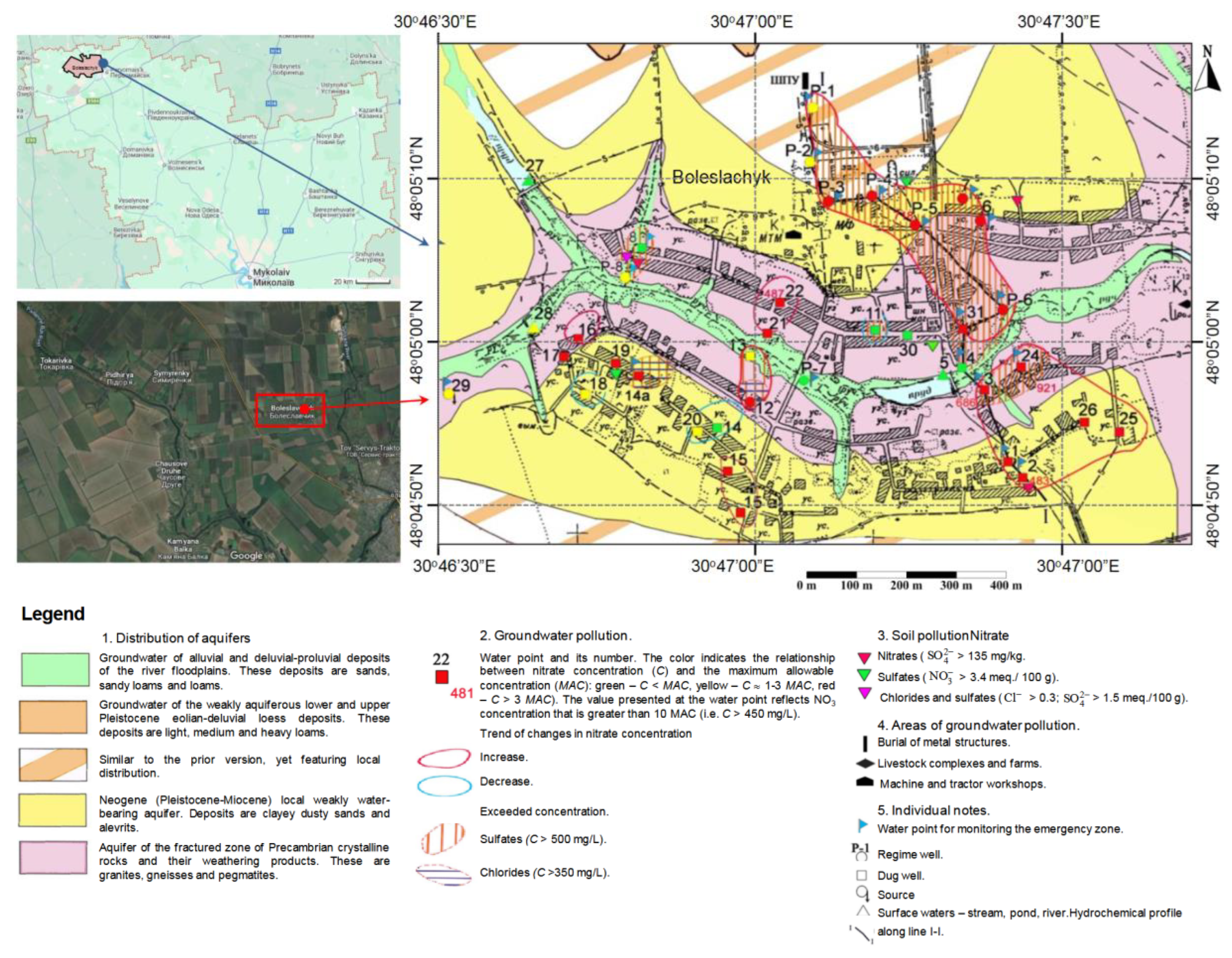
Figure 2.
Component planes for (a) f1, (b) f2, (c) f3, (d) f4, (e) f5, and (f) pH. Orange line: Thnorm (normalized stoichiometric 1:1 threshold); green solid isolines: multiples of the stoichiometric threshold Thnorm; red dotted line: VPC1 (primary evolutionary vector); blue dotted line: VPC2 (secondary evolutionary vector).
Figure 2.
Component planes for (a) f1, (b) f2, (c) f3, (d) f4, (e) f5, and (f) pH. Orange line: Thnorm (normalized stoichiometric 1:1 threshold); green solid isolines: multiples of the stoichiometric threshold Thnorm; red dotted line: VPC1 (primary evolutionary vector); blue dotted line: VPC2 (secondary evolutionary vector).
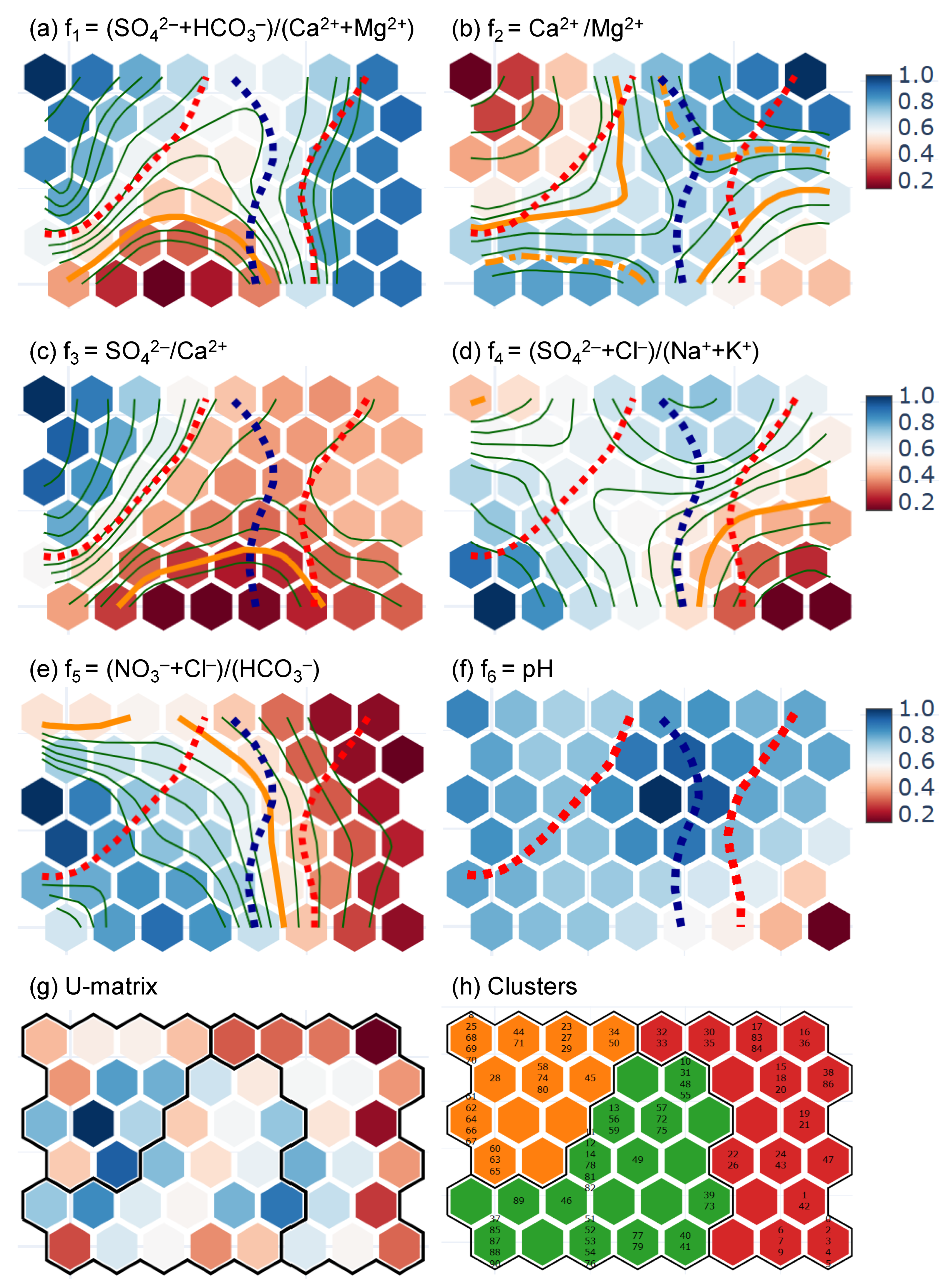
Figure 3.
(a) Silhouette score vs number of clusters, (b) biplot of the two principal components, and (c) dendrogram with node number classified into the respective clusters.
Figure 3.
(a) Silhouette score vs number of clusters, (b) biplot of the two principal components, and (c) dendrogram with node number classified into the respective clusters.
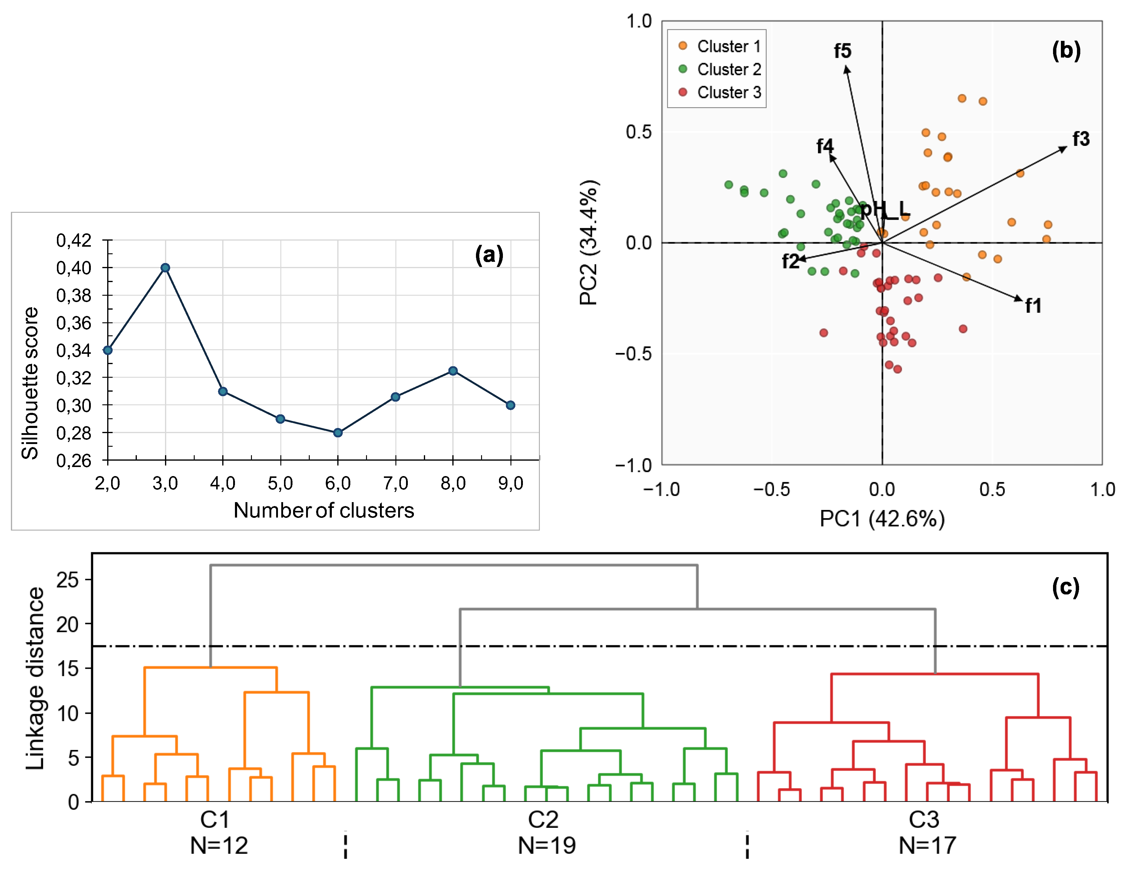
Figure 4.
Spatial distribution of features fi, pH and total dissolved solids (TDS): (a) f1, f2, f4; (b) f3, f5.
Figure 4.
Spatial distribution of features fi, pH and total dissolved solids (TDS): (a) f1, f2, f4; (b) f3, f5.
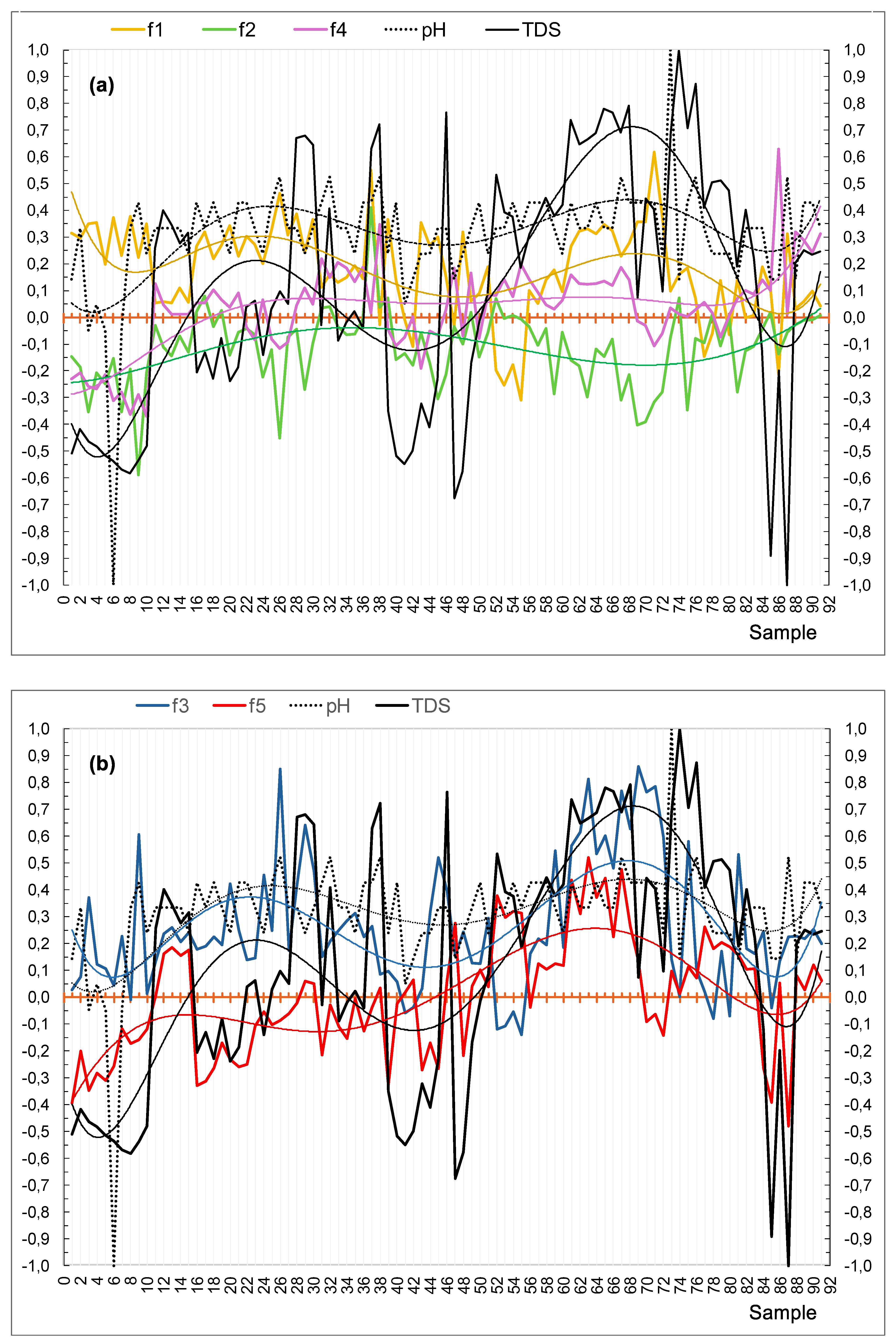
Figure 5.
Validation of Cluster 1 using log-ratio profiles with a single threshold of ln(fi =0).
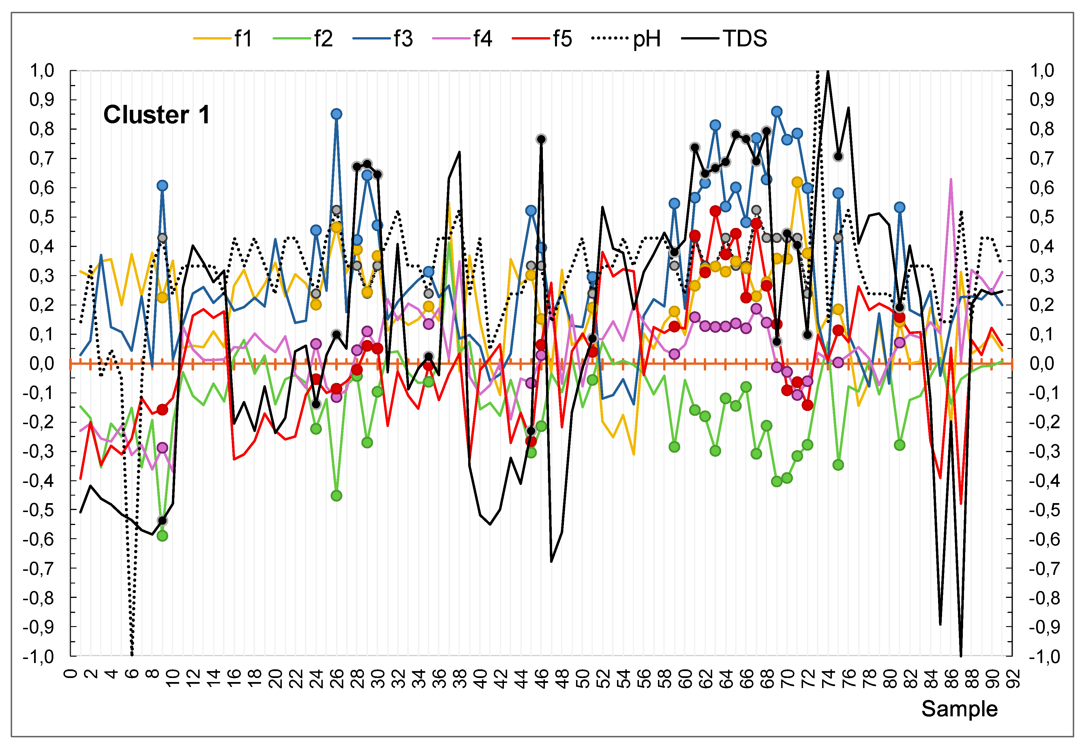
Figure 6.
Validation of Cluster 2 using log-ratio profiles with a single threshold of ln(fi =0).
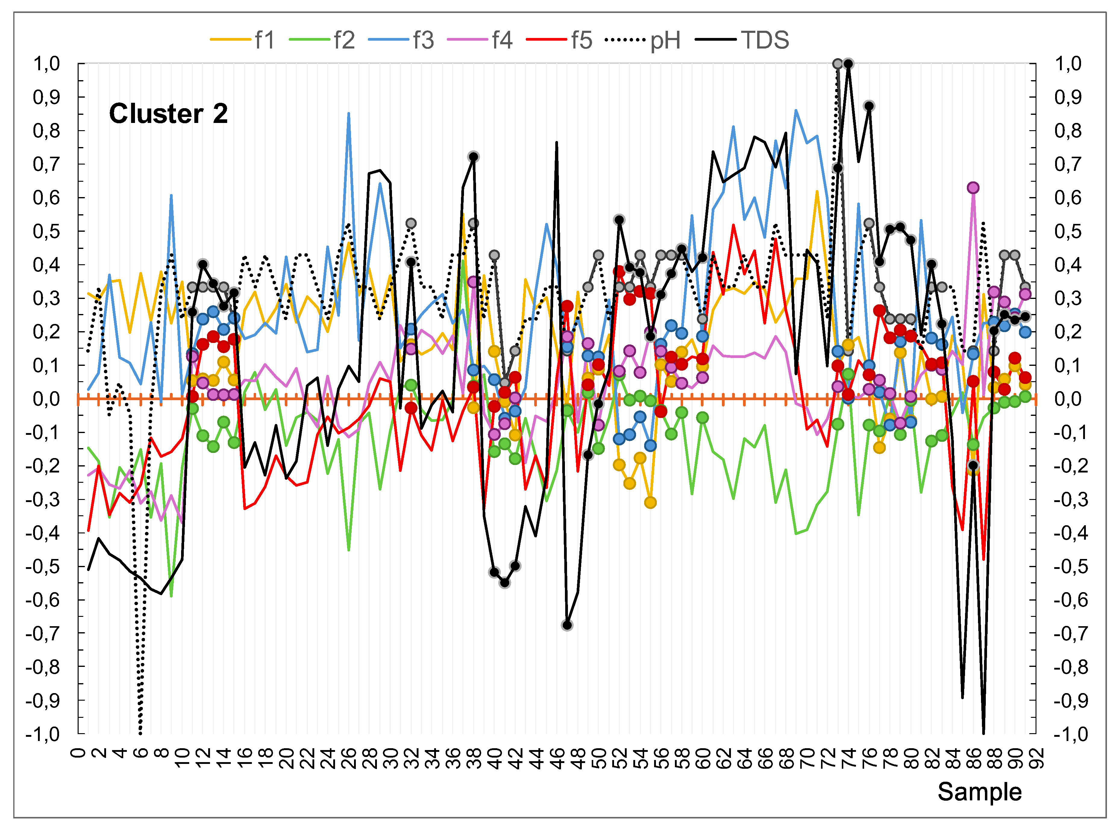
Figure 7.
Validation of Cluster 3 using log-ratio profiles with a single threshold of ln(fi =0).
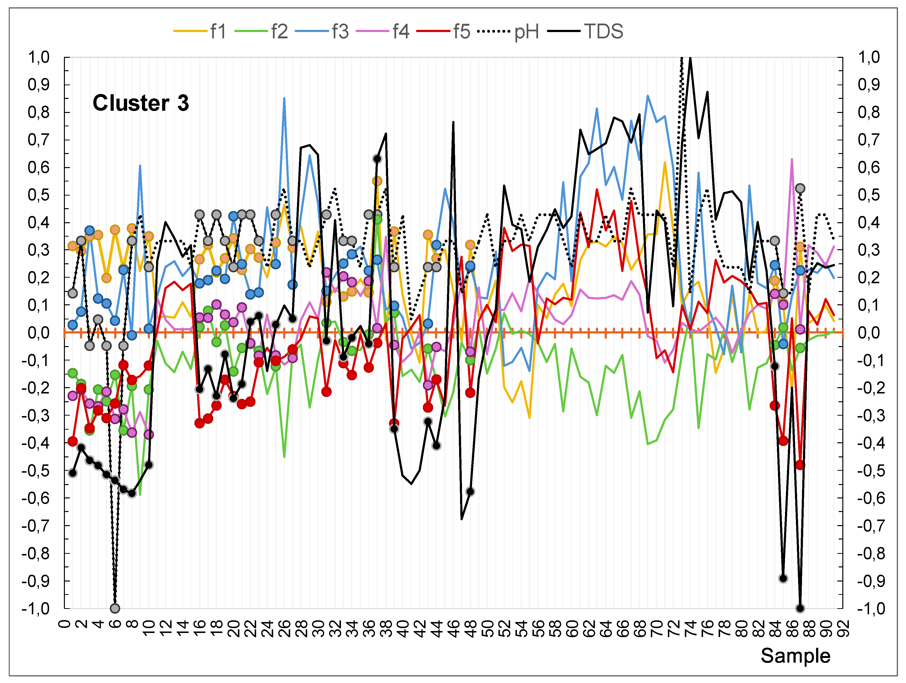

Table 1.
Average chemical composition of groundwater (in mg/L; pH is in the standard unit).
| Variables | Mean | Median | Minimum | Maximum | Standard Deviation |
Coefficient of Variation, % |
|---|---|---|---|---|---|---|
| pH | 7.68 | 7.70 | 6.30 | 8.40 | 0.21 | 3 |
| 15.53 | 14.76 | 2.00 | 27.36 | 5.65 | 36 | |
| 1.72 | 1.64 | 0.10 | 3.04 | 0.62 | 37 | |
| 6.90 | 6.60 | 0.40 | 18.40 | 4.26 | 61 | |
| 10.94 | 11.00 | 1.23 | 19.80 | 4.04 | 37 | |
| 6.83 | 6.60 | 1.00 | 14.80 | 3.20 | 47 | |
| 14.23 | 13.40 | 2.50 | 34.15 | 8.31 | 58 | |
| 10.01 | 10.00 | 2.50 | 16.80 | 3.40 | 34 | |
| 3.93 | 3.14 | 0.01 | 14.83 | 3.78 | 96 |
Table 2.
Hydrogeochemical processes controlling groundwater chemistry and their respective Thnorm criteria.
Table 2.
Hydrogeochemical processes controlling groundwater chemistry and their respective Thnorm criteria.
| Feature | Hydrogeochemical Parameter and Formula | Baseline Conditions before Transformation | Corresponding Thnorm Conditions after Transformation | Hydrogeochemical Process and Interpretation |
|---|---|---|---|---|
| 1 | 2 | 3 | 4 | 5 |
| f1 | f1 > 1 | 0.31 < f1 ≤ 1.0 | Silicate weathering and/or ion exchange | |
| f1 = 1 | f1 =0.31 | Sulfate, carbonate and silicate dissolution | ||
| f1 < 1 | 0.0 ≤ f1 < 0.31 | Carbonate dissolution | ||
| f2 | f2 > 2 | 0.59 ≤ f2 ≤ 1.0 | Silicate weathering | |
| 1 ≤ f2 ≤ 2 | 0.59 ≤ f2 ≤ 0.72 | Calcite dissolution | ||
| f2 < 1 | 0.0 ≤ f2 < 0.59 | Dolomite dissolution / Ion exchange | ||
| f3 | f3 > 1 | 0.14 < f3 ≤ 1.0 | Gypsum dissolution or anthropogenic input of sulfate | |
| f3 = 1 | f3 = 0.14 | Gypsum dissolution | ||
| f3 < 1 | 0.0 ≤ f3 < 0.14 | Calcium containing minerals dissolution | ||
| f4 | f4 > 1 | 0.38 < f4 ≤ 1.0 | Gypsum or anhydrite dissolution / Anthropogenic pollution | |
| f4 = 1 | f4 = 0.38 | Anthropogenic activities | ||
| f4 < 1 | 0.0 ≤ f4 < 0.38 | Silicate weathering dominance | ||
| f5 | f5 ≥1 | 0.48 ≤ f5 ≤ 1.0 | Anthropogenic pollution | |
| f5< 1 | 0.0 ≤ f5 < 0.48 | Carbonate dissolution |
Note: Thnorm represents the normalized stoichiometric 1:1 threshold; the condition where fi(norm) = Thnorm corresponds to the spatial trace of the stoichiometric equality line on the SOM map, marking the exact 1:1 ionic equivalence baseline (ln(1) = 0) before data transformation.
Disclaimer/Publisher’s Note: The statements, opinions and data contained in all publications are solely those of the individual author(s) and contributor(s) and not of MDPI and/or the editor(s). MDPI and/or the editor(s) disclaim responsibility for any injury to people or property resulting from any ideas, methods, instructions or products referred to in the content. |
© 2026 by the authors. Licensee MDPI, Basel, Switzerland. This article is an open access article distributed under the terms and conditions of the Creative Commons Attribution (CC BY) license (http://creativecommons.org/licenses/by/4.0/).
Copyright: This open access article is published under a Creative Commons CC BY 4.0 license, which permit the free download, distribution, and reuse, provided that the author and preprint are cited in any reuse.


