

Submitted:
20 July 2026
Posted:
21 July 2026
You are already at the latest version
Abstract
This article presents an innovative methodology that integrates Dual STATIS analysis with neutrosophic logic to evaluate the stability of the structure of relationships among financial variables in savings and credit cooperatives. The developed approach makes it possible to incorporate the uncertainty present in financial indicators and analyze their temporal evolution. Unlike classical STATIS, which focuses on similarity among cooperatives, the dual approach analyzes the covariance structure among the variables, identifying stable latent dimensions and turning points in the cooperative system. The results reveal patterns of structural stability and significant changes associated with relevant economic events, including the impact of the COVID-19 pandemic. The proposed methodology constitutes a useful alternative for strengthening financial supervision processes and supporting strategic decision-making in the cooperative sector.
Keywords:
dual STATIS
; neutrosophic logic
; multivariate analysis
; savings and credit cooperatives
1. Introduction
The rigorous evaluation of the financial performance of savings and credit cooperatives represents a fundamental element for ensuring the soundness of the financial system and promoting sustainable economic development. In this context, the analysis of financial indicators not only makes it possible to characterize the situation of these institutions, but also to identify behavioral patterns over time, which contributes to strategic decision-making at both the institutional and regulatory levels. In particular, the study of variables such as liquidity, lending activity, profitability, and delinquency is essential for determining trends, risks, and efficiency levels within Ecuador’s Popular and Solidarity Financial Sector.
In the field of multivariate analysis, techniques aimed at data visualization and dimensionality reduction represent continuously developing lines of research. Among the most relevant methods is principal component analysis (PCA), which has become an essential method for structuring, classifying, and understanding the variables and study units that make up the dataset [1]. A significant contribution to this field was the proposal of Biplot Methods [2], formulated as a resource that enables the multivariate graphical representation of individuals and variables in a low-dimensional space, thereby allowing the identification and analysis of latent patterns. This contribution promoted new lines of research in multivariate visualization advances, with the HJ-Biplot [3,4] standing out; it extends Gabriel’s initial approach by integrating the characteristics of the GH-Biplot and the JK-Biplot in order to obtain a simultaneous representation with optimal representation quality [5].
In the classical multivariate approach, data are organized into two-dimensional matrices , where corresponds to the units of analysis or individuals and to the set of observed variables. However, in various applied research settings, empirical information incorporates measurements of multiple variables obtained from different individuals over time and under different experimental conditions, leading to three-mode data structures formalized as three-dimensional arrays ; this configuration considerably increases the level of complexity of the analysis and requires the adoption of advanced techniques capable of rigorously modeling the interrelationships, dependencies, and covariation patterns that arise among the three dimensions.
From a historical perspective, financial analysis has moved from descriptive and univariate approaches toward more robust methodologies from multivariate statistics, capable of jointly examining multiple indicators and periods. In this regard, the need to analyze complex data structures organized at different points in time has promoted the use of three-way techniques. Among these, the STATIS method derives from the French expression “Structuration des Tableaux à Trois Indices de la Statistique” [6,7], which refers to the study of data organized in three dimensions. This method belongs to the set of three-way analysis methods and is considered an extension of principal component analysis [8], whose objective is to study a set of variables observed on the same individuals. This approach makes it possible to obtain a global structure known as the compromise, which is derived from principal component analysis. On this common basis, the different original tables can be projected into the same space, facilitating comparative analysis to identify similarities and differences among the datasets [9].
In the context of this research, these approaches are particularly useful for analyzing the evolution of economic and financial variables, facilitating the detection of structural dynamics. Likewise, recent studies have developed generalizations of principal component analysis for three-dimensional data structures, thereby strengthening the capabilities of multivariate analysis [10,11].
Dual STATIS is a three-way multivariate method that makes it possible to analyze phenomena in which individuals and variables interact over time. This is valuable for quality-of-life analysis because it enables a comprehensive understanding of the information through graphical representations. In addition, its versatility in allowing the simultaneous analysis of three dimensions has favored its application in various fields, such as engineering [12], mathematics [13,14], and biological sciences research [15]. Furthermore, both STATIS and Dual STATIS are part of three-way multivariate techniques: whereas STATIS is aimed at identifying similarities among individuals in different time periods, Dual STATIS analyzes covariation relationships among variables.
Within this conceptual framework, the main extensions of the STATIS method are described. These include X-STATIS or partial triadic analysis (PTA), applied when the different tables contain the same variables measured on the same set of observations [16]; COVSTATIS, focused on the analysis of multiple covariance matrices obtained from the same observations [17]; DISTATIS, which makes it possible to work with distance matrices and extends multidimensional scaling to three-way structures [18]; Canonical-STATIS (CANO-STATIS), which integrates discriminant analysis with DISTATIS to address multitable problems [19]; and Power-STATIS, which introduces alternative criteria for estimating the optimal table weights [20]. The STATIS framework also includes extensions such as (K+1)-STATIS or external STATIS, which enables the joint analysis of multiple tables together with an additional set, and Double-STATIS (DO-ACT), which extends the approach to the simultaneous analysis of two groups of tables [21]. Extensions aimed at more complex data structures have also been developed in this field, including adaptations for qualitative variables and categorical data. In this regard, CATATIS is aimed at the analysis of categorical variables associated with individuals, whereas CLUSTATIS makes it possible to group homogeneous datasets and relate them to a consensus structure [22,23,24].
Nevertheless, traditional approaches have limitations when data are affected by uncertainty, imprecision, or variability in their interpretation, such as fluctuations in the economic environment that introduce levels of indeterminacy that are not adequately captured by classical methods. Under this approach, neutrosophic statistical methods are aimed at studying data that present uncertainty, known as neutrosophic data. In this context, fundamental parameters such as sample size may not be precisely defined, reflecting the approach’s ability to model incomplete or imprecise information [25,26,27].
From an applied perspective, neutrosophic numbers have been used in various disciplines, such as rock engineering [28] and educational contexts [29]. In addition, neutrosophic theory has been widely applied in the development of correlation and similarity measures, such as correlation coefficients for interval neutrosophic sets [30] and cosine similarity measures for disease diagnosis [31]. These tools have made it possible to address problems in areas such as medicine, particularly the diagnosis of complex disorders, as well as the optimization of structures such as minimum spanning trees in neutrosophic environments [32].
Furthermore, in the field of artificial intelligence and data analysis, methods such as the neutrosophic c-means clustering algorithm [33] have been proposed, which optimizes the classification of information in contexts characterized by uncertainty. Neutrosophic statistics has also been applied in post hoc tests for multiple mean comparisons [34], as well as in the study of physical phenomena, for example, the analysis of material resistance under temperature variations [35], demonstrating its applicability in different scientific fields.
Ultimately, this approach has also been incorporated into the business and industrial sectors, particularly in the evaluation of practices related to green supply chain management through neutrosophic methodologies [36]. This demonstrates its ability to support strategic decision-making processes in scenarios involving uncertain information. Taken together, these advances highlight the growing importance of neutrosophic statistics as a comprehensive tool for handling complex data in various contexts.
Within this framework, a relevant question arises: How does the neutrosophic Dual STATIS method make it possible to analyze the temporal evolution of structural relationships among financial variables while considering the uncertainty present in the cooperative system?
To address this challenge, the present study proposes the application of the Neutrosophic Dual STATIS method as an innovative methodology that makes it possible to integrate neutrosophic logic into multivariate analysis. This approach facilitates the modeling of information in terms of truth, indeterminacy, and falsity, providing a more complete representation of financial data. Specifically, the relationships among financial indicators are analyzed by explicitly incorporating the levels of uncertainty and indeterminacy present in the financial information of savings and credit cooperatives.
2. Materials and Methods
2.1. Preparation of Neutrosophic Data
2.1.1. Multi-Table Structuring of the Longitudinal Dataset
The study is based on a longitudinal design covering the 2016-2023 period, with the information structured into eight consecutive annual tables. Each table (with) integrates the financial assessments of savings and credit cooperatives through fundamental financial indicators. The multitable structure makes it possible to analyze the temporal dynamics of the cooperative sector, where each year represents a specific configuration of the financial system under analysis.
The variables analyzed include DEP, which represents total deposits and makes it possible to measure size and deposit-taking capacity; SCC, which reflects lending activity; INTFIN, which indicates operating efficiency; LIQCOR, which indicates short-term solvency; MORAMP, which expresses the delinquency rate associated with credit risk; ROA, which evaluates return on assets as an efficiency indicator; and ROE, which measures return on equity.
2.1.2. Neutrosophic Transformation of Financial Variables
The methodological innovation is based on transforming traditional financial values into single-valued neutrosophic numbers represented as triplets . This procedure makes it possible to capture not only the magnitude of each indicator, but also the degrees of indeterminacy and inconsistency inherent in cooperative financial systems.
Rationale for the Neutrosophic Transformation:
Indeterminacy combines two components: local volatility , calculated as the average of the absolute variations with respect to the previous and following years and normalized to [0,1]; and sectoral deviation , calculated as the absolute distance between the cooperative’s value and the sector median in standard deviation units. The weights assigned to both components vary according to the nature of each variable.
Profitability (ROA and ROE):
Truth is defined through linear normalization, and indeterminacy is calculated as:
Greater weight is assigned to temporal volatility because a cooperative’s profitability responds mainly to internal management decisions over time rather than to its relative position within the sector. [37,38].
Delinquency Risk (MORAMP): For delinquency, a low value is desirable:
Tijk=1−xijk−míni(xijk)máxi(xijk)−míni(xijk)
Delinquency has a stronger sectoral component than profitability, because credit risk responds in part to cycles and conditions shared by the cooperative system [37].
Operating Efficiency (INTFIN):
The efficiency optimum is located around , consistent with the official definition of the financial intermediation indicator for the popular and solidarity financial system [37], subject to the restriction. Falsity is defined as:
2.1.3. Neutrosophic Score
The score function proposed by [41] is applied.
Substitution yields:
2.2. Phase 2: Neutrosophic Dual Interstructure Analysis
2.2.1. Centering and Scaling
To prevent variables with larger scales from exerting a dominant influence on the analysis results [10], the data matrices are subjected to a centering and scaling process defined by the following expression:
where represents the vector of variable means and corresponds to a diagonal matrix composed of their respective variances. This procedure makes it possible to homogenize the contribution of each variable within the multivariate analysis, ensuring an appropriate comparison among them.
2.2.2. Dual Scalar Product Matrices
The similarity matrices among variables are calculated for each year, where is a p × p matrix, with p = 7, the number of financial variables, containing the covariances among the centered and scaled neutrosophic scores of the variables for year k and capturing the structure of relationships among the financial variables in that specific period.
2.2.3. Calculation of the Neutrosophic Dual RV Coefficient
The RV coefficient, introduced by Escoufier [16], is a measure used to evaluate the degree of similarity between two data configurations or structures. In its dual version, this coefficient makes it possible to compare the structural relationship between matrices, taking values between 0 and 1, where values close to 1 indicate high structural similarity between the analyzed structures, whereas values close to 0 reflect low correspondence between them.
2.2.4. Construction of the Temporal Similarity Matrix
The matrix of dimension is constructed
2.3. Phase 3: Construction of the Neutrosophic Dual Compromise
The weight vector is calculated from the first eigenvector of matrix R, where is the first eigenvector of matrix R associated with its dominant eigenvalue . Each component quantifies the relative contribution of year k to the consensus structure, so that the years whose configuration of relationships among variables is more representative of the general pattern of the period will receive a greater weight in the dual compromise.
The weights are then normalized so that their sum is equal to one.
2.3.1. Construction of the Compromise Matrix
The compromise matrix is obtained through the convex combination of matrices , using the previously calculated weights as the weighting factors.
This matrix summarizes the information shared among all study periods and reflects the consensus structure of the relationships among the financial variables.
2.4. Phase 4: Dual Intrastructure
Principal component analysis of the compromise matrix is performed:
where U is the eigenvector matrix and Λ is a diagonal matrix containing the eigenvalues
2.4.1. Variable Coordinates
The principal coordinates of the variables within the compromise space are calculated using the following expression:
The inertia explained by each dimension is calculated as:
2.4.2. Projection of Individual Years
To examine the temporal dynamics of the variable structure, each matrix is projected onto the compromise space. The corresponding coordinates are determined using the following expression:
The coordinates obtained make it possible to represent the evolution of the relational structure among the variables over time. Likewise, they facilitate the identification and visualization of the trajectories described by these relationships during the period analyzed.
2.5. Phase 5: Interpretation of Dimensions
The dimensions of the compromise space are interpreted in financial terms:
Dimension 1 (Profitability vs. Efficiency): Separates profitability variables (ROA, ROE) from efficiency indicators (INTFIN).
Dimension 2 (Risk vs. Size): Contrasts risk indicators (MORAMP)
with size and credit variables (DEP, SCC).
Dimension 3 (Specific Liquidity): Captures the particular structure of liquidity (LIQCOR).
2.5.1. Temporal Stability Analysis
The stability of the variable structure is evaluated through the distance between annual projections, calculated for each pair of years within the study period.
where denotes the Frobenius norm and is the number of retained dimensions.
The analysis was performed using the R statistical software. Because the neutrosophic extension of Dual STATIS does not exist as a specialized package, custom routines were developed for each phase of the process: data reading and organization with readxl and tidyr, calculation of neutrosophic transformations with dplyr, purrr, and stringr, and graph production with ggplot2 and ggrepel. The complete code can be accessed at: https://github.com/GTX-Dev/Script-.git
3. Results of the Neutrosophic Dual STATIS Model
Based on the annual tables corresponding to the 2016–2023 period, a Neutrosophic Dual STATIS model was developed to synthesize the consensus structure of relationships among financial variables, simultaneously integrating the observed financial information and the degree of indeterminacy associated with each variable and cooperative. Unlike the classical STATIS method, which focuses its analysis on similarities among cooperatives, the dual approach is oriented toward studying the relationships among financial indicators and the way in which this relationship structure changes and evolves over time.
The analytical strategy made it possible to examine three complementary levels: temporal interstructure through the neutrosophic dual RV similarity matrix, the compromise structure through factorial analysis of the consensus among variables, and temporal intrastructure through the trajectories of the variables projected into the dual compromise space.
3.1. Dual Temporal Interstructure: Similarity Among Years and STATIS Weights
The temporal similarity matrix shows that the structural relationships among the variables did not remain homogeneous throughout the period analyzed, but instead exhibited different levels of proximity and structural stability. In general terms, the greatest similarities were recorded in nearby years, with a pattern of high temporal coherence.

Table 1.
Neutrosophic dual RV temporal similarity matrix among years.
| Year | 2016 | 2017 | 2018 | 2019 | 2020 | 2021 | 2022 | 2023 |
|---|---|---|---|---|---|---|---|---|
| 2016 | 1.000 | 0.925 | 0.828 | 0.836 | 0.849 | 0.881 | 0.892 | 0.865 |
| 2017 | 0.925 | 1.000 | 0.875 | 0.861 | 0.891 | 0.929 | 0.929 | 0.798 |
| 2018 | 0.828 | 0.875 | 1.000 | 0.844 | 0.810 | 0.881 | 0.926 | 0.893 |
| 2019 | 0.836 | 0.861 | 0.844 | 1.000 | 0.894 | 0.802 | 0.813 | 0.781 |
| 2020 | 0.849 | 0.891 | 0.810 | 0.894 | 1.000 | 0.881 | 0.889 | 0.812 |
| 2021 | 0.881 | 0.929 | 0.881 | 0.802 | 0.881 | 1.000 | 0.939 | 0.839 |
| 2022 | 0.892 | 0.929 | 0.926 | 0.813 | 0.889 | 0.939 | 1.000 | 0.916 |
| 2023 | 0.865 | 0.798 | 0.893 | 0.781 | 0.812 | 0.839 | 0.916 | 1.000 |
The highest dual RV coefficients were recorded between 2021 and 2022 (RV= 0.939), between 2017 and 2022 (RV= 0.929), between 2017 and 2021 (RV= 0.929), and between 2018 and 2022 (RV= 0.926). These results suggest that the structure of relationships among financial variables remained relatively stable during certain periods, especially 2017-2018 and 2021-2022.
Conversely, the lowest similarities were observed between 2019 and 2023 (RV = 0.781), between 2017 and 2023 (RV = 0.798), between 2021 and 2019 (RV = 0.802), and between 2018 and 2020 (RV = 0.81). These low associations reflect that the system of financial relationships experienced relevant reconfigurations over time, especially when contrasting the period prior to the COVID-19 pandemic with the post-pandemic structure (2023).
The compromise weights were derived from the RV matrix and calculated from its first eigenvector, as described in Section 2.3; they quantify the degree of agreement between the relationship structure of each year and the general consensus for the 2016-2023 period.”
The year with the highest weight was 2022 (0.12921), followed by 2017 (0,12752), 2021 (0,12655), and 2016 (0,12512). In contrast, 2019 had the lowest weight (0.12063), followed by 2023 (0.12201) and 2018 (0.12478), suggesting that the relationship structure among variables in 2022 is the most representative of the general consensus, whereas the pre-pandemic year (2019) shows a more atypical structure. The low representativeness of 2023 could indicate that the pandemic-related reconfiguration process has not yet been fully consolidated.
Table 2.
Neutrosophic STATIS compromise weights by year.
| Year | Weight |
|---|---|
| 2016 | 0.12512 |
| 2017 | 0.12752 |
| 2018 | 0.12478 |
| 2019 | 0.12063 |
| 2020 | 0.12418 |
| 2021 | 0.12655 |
| 2022 | 0.12921 |
| 2023 | 0.12201 |
3.2. Dual Compromise Inertia and Quality of Representation
The dual compromise analysis showed that the first three dimensions capture an important proportion of the consensus structure of relationships among variables. The first dimension had an eigenvalue of 53.034 and explained 31.57% of the total inertia, whereas the second reached an eigenvalue of 28.749 and explained 17.11%. Together, both dimensions accounted for 48.68% of the compromise variation. The third dimension had an eigenvalue of 27.323, corresponding to 16.26% of the total inertia. Although the cumulative inertia of the first two dimensions does not capture the full complexity of the system, it is sufficient to obtain an interpretable two-dimensional representation of the compromise. In addition, the magnitude of the third dimension suggests the existence of relevant additional heterogeneity in the financial relationships.
Table 3.
Eigenvalues and inertia explained by the neutrosophic dual STATIS compromise.
| Dimension | Eigenvalue | Inertia (%) |
|---|---|---|
| Dim 1 | 53.0342 | 31.57 |
| Dim 2 | 28.7497 | 17.11 |
| Dim 3 | 27.3229 | 16.26 |
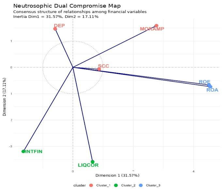
3.3. Dual Compromise Map: Structure of Relationships among Variables
The dual compromise map shows a clear segmentation of the relationships among the seven financial variables analyzed. The projection of the variables in the consensus space makes it possible to identify patterns of association, opposition, and independence.
Figure 1.
Compromise map of the neutrosophic dual STATIS model: consensus structure of relationships among financial variables (authors’ own elaboration in R, ggplot2 package).
Figure 1.
Compromise map of the neutrosophic dual STATIS model: consensus structure of relationships among financial variables (authors’ own elaboration in R, ggplot2 package).
Interpretation of Dimension 1 (31.57% inertia)
The first dimension is dominated by a strong contrast between profitability variables and financial efficiency. At the positive end of Dim1 are ROA (4.558) and ROE (4.512), followed by MORAMP (2.770). At the negative end is INTFIN (-1.640), whereas DEP (-0.589), SCC (0.872), and LIQCOR (0.654) have coordinates close to the origin.
This pattern suggests that Dimension 1 summarizes a structural tension between profitability-risk and financial efficiency. Cooperatives with high levels of ROA and ROE tend to have a negative relationship with the INTFIN efficiency indicator, which could be interpreted as a trade-off between profitability and operating efficiency.
The second-dimension separates liquidity and solvency variables from profitability variables. At the positive end of Dim2 are DEP (1.466) and MORAMP (1.585), whereas LIQCOR (-3.590) and INTFIN (-3.195) are positioned at the negative end. ROA (-0.735) and ROE (-0.667) show moderately negative coordinates. This behavior indicates that Dimension 2 distinguishes between profiles associated with size and risk (DEP, MORAMP) and profiles closer to liquidity and efficiency (LIQCOR, INTFIN). The opposition between DEP and LIQCOR suggests that larger cooperatives (deposits) tend to have lower liquidity levels, possibly because of a more diversified asset structure.
3.4. Structure of the Variables in the Compromise
The cluster analysis (k = 3) made it possible to identify three groups of variables with similar relational behavior:
Cluster 1 (Profitability-Risk): Composed of ROA, ROE, MORAMP, DEP, and SCC. This group represents the classical core of financial analysis, where profitability and risk covary positively, while size (DEP, SCC) shows a moderate association.
Cluster 2 (Liquidity-Efficiency): Composed of LIQCOR and INTFIN. These variables are projected in the negative region of Dim2, indicating a structural association between liquidity and operating efficiency.
Table 4.
Coordinates of the variables in the dual compromise space.
| Variable | Dim1 | Dim2 | Dim3 | Contribution Dim1-Dim2 | Cluster |
|---|---|---|---|---|---|
| ROA | 4.558 | -0.735 | -0.616 | 5.293 | Cluster 1 |
| ROE | 4.512 | -0.667 | 0.001 | 5.179 | Cluster 1 |
| MORAMP | 2.770 | 1.585 | 0.590 | 4.355 | Cluster 1 |
| DEP | -0.589 | 1.466 | 3.479 | 2.055 | Cluster 1 |
| SCC | 0.872 | -0.071 | 3.536 | 0.943 | Cluster 1 |
| INTFIN | -1.640 | -3.195 | 0.451 | 4.835 | Cluster 2 |
| LIQCOR | 0.654 | -3.590 | 1.336 | 4.244 | Cluster 2 |
3.5. Temporal Trajectories of the Cooperatives
The temporal projections of the variables make it possible to understand how the position of each financial indicator evolved in the compromise space during the 2016-2023 period; this analysis is fundamental for identifying changes in the structural relationships among the variables.
Figure 2.
Temporal trajectories of the cooperatives in the compromise space.
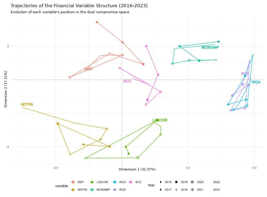
The profitability variables (ROA and ROE) show stable behavior throughout the entire period. Their coordinates in Dim1 remain consistently high (between 4.0 and 4.9), while in Dim2 they fluctuate moderately between -1.8 and 0.5. This stability suggests that profitability is a solid financial construct whose relationship with the other variables has remained relatively constant in the face of economic changes.
In addition, the ROA and ROE trajectories are nearly parallel, confirming their strong structural association. The year 2020 shows a slight shift toward more negative values in Dim2 for both variables, possibly reflecting the impact of the pandemic on sector profitability.
The delinquency variable (MORAMP) exhibits a more dynamic trajectory. Between 2016 and 2018, MORAMP was located in the positive region of Dim2 (between 1.14 and 2.27), but from 2019 onward it shows a gradual shift toward negative Dim2 values, reaching -1.73 in 2023. This change suggests a reconfiguration in the relationship between credit risk and the other financial variables, possibly associated with changes in post-pandemic credit policies.
INTFIN shows the most differentiated and variable trajectory. In 2016, it was located in the negative region of Dim1 (-1.45) and the highly negative region of Dim2 (-3.86). During the 2016-2019 period, INTFIN shifted toward even more negative values in Dim2 (reaching -4.45 in 2019), and then gradually recovered to -1.64 in 2023. This pattern indicates that the relationship between financial efficiency and the other variables has been particularly sensitive to economic conditions, with a point of maximum separation during the years preceding the pandemic.
LIQCOR shows a complex trajectory. In 2016, it was located in the highly negative region of Dim2 (-4.41) and the moderately positive region of Dim1 (0.26). During 2017-2019, LIQCOR shifted toward less negative values in Dim2, reaching -2.58 in 2021. This behavior suggests that liquidity has strengthened its structural association with other variables over time. DEP and SCC show relatively stable trajectories in the Dim1-Dim2 plane, although with significant shifts in the third dimension (not represented). Both indicators maintain positive coordinates in Dim3 (between 3.1 and 3.9), suggesting that they share a common latent dimension related to institutional size. The proximity between DEP and SCC in the compromise space confirms the strong structural relationship between both variables, which is consistent with the nature and definition of these indicators.
3.6. Evolution of Key Correlations over Time
Figure 4 presents the evolution of correlations between specific pairs of variables, making it possible to identify changes in the most relevant structural relationships.
Figure 3.
Evolution of correlations among financial variables.
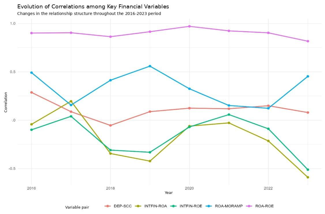
The correlation between ROA and ROE remains consistently high throughout the period, fluctuating between 0.85 and 0.98, with a maximum in 2020 (0.98) and a minimum in 2018 (0.85). This high and stable correlation confirms that both profitability indicators capture complementary but strongly aligned dimensions of financial performance. The correlation between deposits (DEP) and lending activity (SCC) shows a downward trend, moving from 0.28 in 2016 to -0.02 in 2018, and then recovering moderately to 0.17-0.19 in the 2020-2023 period. This pattern suggests a temporary weakening in the relationship between size and credit during 2018-2019, possibly associated with regulatory or structural changes in the sector.
The correlation between efficiency (INTFIN) and return on equity (ROE) shows a downward trend, moving from 0.45 in 2016 to 0.20 in 2021 and then recovering slightly to 0.22 in 2022. This behavior indicates that the relationship between operating efficiency and return on equity has weakened in recent years, which could reflect a greater influence of external factors on profitability. On the other hand, the correlation between profitability (ROA) and delinquency (MORAMP) is systematically negative (fluctuating between -0.10 and -0.35), confirming the expected inverse relationship: the higher the delinquency, the lower the profitability. The most negative value is observed in 2019 (-0.35) and 2022 (-0.30), whereas 2017 shows the least negative correlation (-0.10). This pattern suggests that the negative impact of delinquency on profitability has intensified in recent years.
Uncertainty by Variable.
Table 5 presents the average indeterminacy levels () for each financial variable, calculated from the weighted combination of local volatility and sectoral deviation described in Section 2.1.2; higher indeterminacy values reflect greater temporal instability or greater dispersion relative to the sectoral behavior of the corresponding variable.
The variables with the greatest uncertainty are MORAMP (0.405), LIQCOR (0.386), and SCC (0.379). This pattern indicates that delinquency, liquidity, and lending activity are dimensions that are particularly sensitive to temporal volatility and sectoral deviation. In contrast, ROA (0.315) and ROE (0.321) present the lowest uncertainties, suggesting that profitability is a more stable and reliable indicator in the context of the cooperative sector.
Uncertainty by Cooperative
Table 6 presents the cooperatives with the highest average uncertainty in the dual analysis.
SPMEC stands out as the cooperative with the highest average uncertainty (0.425), followed by JEP (0.408), ADV (0.399), and RIO (0.392). This result confirms findings from the classical analysis and suggests that these entities exhibit more volatile or less predictable financial behavior in terms of their structural relationships with the system.
4. Discussion
The results obtained show that incorporating the neutrosophic approach into the Dual STATIS method makes it possible to complement traditional multivariate analysis in contexts characterized by uncertainty and incomplete information. Although the STATIS method has been widely used for the analysis of multitable structures and three-way data [10,18], these classical approaches do not explicitly incorporate levels of indeterminacy associated with the analyzed information. In this context, the proposal developed in this research presents a methodological extension aimed at integrating uncertainty into the structural analysis of financial relationships.
From a temporal perspective, the neutrosophic dual RV matrix showed high levels of similarity between consecutive years, especially between 2021 and 2022, demonstrating relative stability in the structure of financial relationships in the cooperative system during the post-pandemic period. However, the lower similarities observed between 2019 and 2023 suggest important changes in the sector’s financial structure, possibly associated with the economic impact of the health crisis and subsequent adjustments in credit and financial management policies. These results are consistent with previous research using the STATIS approach, in which temporal structures make it possible to identify periods of stability and structural changes in complex multivariate systems [10,19].
Likewise, the compromise analysis made it possible to identify that dimensions associated with profitability, risk, and financial efficiency organize a large part of the cooperative system’s consensus structure. The opposition observed between ROA-ROE and INTFIN suggests the existence of an inverse relationship between profitability and operating efficiency, indicating that higher profitability levels are not necessarily accompanied by equivalent increases in financial efficiency. Similarly, the negative relationship observed between delinquency and profitability confirms the adverse effect of credit risk on the financial performance of cooperatives.
With respect to temporal trajectories, variables such as ROA and ROE display relatively stable behavior throughout the period analyzed, whereas MORAMP and INTFIN show greater changes in the compromise space. This suggests that profitability constitutes a more consistent financial dimension, whereas variables associated with risk and efficiency are more sensitive to economic and regulatory changes. In addition, the progressive shift of MORAMP after 2020 could be related to changes in credit-risk dynamics within the cooperative sector.
One of the main contributions of this study is the explicit incorporation of indeterminacy through neutrosophic numbers. Unlike conventional statistical approaches, neutrosophic statistics makes it possible to incorporate truth, falsity, and indeterminacy simultaneously into the data [26,27,28]. In this study, the MORAMP, LIQCOR, and SCC variables concentrated the highest levels of uncertainty, showing that dimensions related to risk, liquidity, and solvency are more sensitive to financial volatility and structural changes in the economic environment. These results show that uncertainty is not distributed homogeneously among variables or cooperatives.
Likewise, cooperatives such as SPMEC, JEP, and ADV recorded higher average uncertainty levels, which could be associated with more variable or less stable financial behavior within the cooperative system. In this regard, the neutrosophic approach provides additional information that cannot be captured by classical methods, making it possible to identify not only structural patterns but also differentiated levels of indeterminacy among financial institutions.
5. Conclusions
This research proposed a neutrosophic extension of the Dual STATIS method [42] for the analysis of multivariate structures under uncertainty, applied to the Ecuadorian cooperative financial system during the 2016–2023 period. The results show that incorporating neutrosophic numbers makes it possible to consider not only the observed information but also the levels of indeterminacy associated with the financial information, providing a more comprehensive perspective than traditional statistical approaches.
In methodological terms, the model made it possible to adapt the RV coefficient, compromise analysis, and dual representation to the neutrosophic framework while maintaining the factorial interpretation of the classical STATIS method. In addition, the methodology demonstrated an adequate capacity to synthesize complex temporal information and detect changes in the financial structure of the cooperative system.
The empirical analysis showed that the financial structure of the cooperatives varies over time, especially in the years following the pandemic. Likewise, variables such as profitability, delinquency, and institutional size emerged as important dimensions within the system’s consensus configuration. Similarly, the temporal trajectories showed that not all cooperatives maintain similar behavior, as some display more stable patterns while others show more noticeable changes in their financial structure.
The uncertainty component made it possible to identify that variables such as MORAMP, LIQCOR, and SCC present higher levels of indeterminacy, suggesting that dimensions related to risk, liquidity, and lending activity are more sensitive to financial and economic changes. In addition, certain cooperatives recorded high average uncertainty levels, demonstrating less stable behavior within the cooperative system. In general, the results show that Neutrosophic Dual STATIS represents a useful tool for financial analysis in environments characterized by uncertainty and variable information. Its capacity to integrate structural relationships, temporal evolution, and indeterminacy expands the possible applications of neutrosophic statistics in multivariate studies and in processes that support financial decision-making.
Author Contributions
Conceptualization, G.V.B.-C. and P.G.-V.; methodology, P.G.-V., P.V.-G. and G.V.B.-C.; formal analysis, P.G.-V. and P.V.-G.; investigation, G.V.B.-C. and C.C.G.; validation, P.G.-V. and P.V.-G.; data curation, G.V.B.-C. and C.C.G.; software, P.V.-G. and G.V.B.-C.; visualization, G.V.B.-C. and P.V.-G.; resources, G.V.B.-C. and C.C.G.; writing—original draft preparation, G.V.B.-C.; writing—review and editing, P.G.-V., P.V.-G. and C.C.G.; supervision, P.G.-V.; project administration, G.V.B.-C. All authors have read and agreed to the published version of the manuscript.
Funding
This research received no external funding.
Institutional Review Board Statement
Not applicable.
Informed Consent Statement
Not applicable.
Data Availability Statement
The data presented in this study are available on request from the corresponding author.
Acknowledgments
The authors are grateful to the Department of Statistics at the University of Salamanca (USAL) and to Universidad Estatal de Milagro (UNEMI) for their support in the publication of this work.
Conflicts of Interest
The authors declare no conflicts of interest.
Appendices
Appendix 1: Segment 1 Cooperatives of the Popular and Solidarity Financial System
| Cooperative | Acronym |
| Cooperative of Savings and Credit Juventud Ecuatoriana Progresista Limited | JEP |
| Cooperative of Savings and Credit Jardín Azuayo Limited | JA |
| Cooperative of Savings and Credit National Police Limited | PN |
| Cooperative of Savings and Credit 29 de Octubre Limited | 29O |
| Cooperative of Savings and Credit Cooprogreso Limited | CP |
| Cooperative of Savings and Credit Oscus Limited | OSC |
| Cooperative of Savings and Credit San Francisco Limited | SF |
| Cooperative of Savings and Credit Vicentina Manuel Esteban Godoy Ortega Limited | VMEGO |
| Cooperative of Savings and Credit Riobamba Limited | RIO |
| Cooperative of Savings and Credit Alianza del Valle Limited | ADV |
| Cooperative of Savings and Credit of the Small Enterprise of Cotopaxi Limited | PEC |
| Cooperative of Savings and Credit Mushuc Runa Limited | MR |
| Cooperative of Savings and Credit Andalucía Limited | AND |
| Cooperative of Savings and Credit of the Small Enterprise Biblián Limited | PEB |
| Cooperative of Savings and Credit Atuntaqui Limited | ATQ |
| Cooperative of Savings and Credit El Sagrario Limited | ES |
| Cooperative of Savings and Credit Chamber of Commerce of Ambato Limited | CCA |
| Cooperative of Savings and Credit 23 de Julio Limited | 23J |
| Cooperative of Savings and Credit San José Limited | SJ |
| Cooperative of Savings and Credit Pablo Muñoz Vega Limited | PMV |
| Cooperative of Savings and Credit Tulcán Limited | TUL |
| Cooperative of Savings and Credit of the Public Servants of the Ministry of Education and Culture | SPMEC |
| Cooperative of Savings and Credit Pilahuín Tío Limited | PT |
| Cooperative of Savings and Credit Santa Rosa Limited | SR |
| Cooperative of Savings and Credit of the Small Enterprise of Pastaza Limited | PEP |
References
- Hached, M.; Jbilou, K.; Koukouvinos, C.; Mitrouli, M. A multidimensional principal component analysis via the C-product Golub–Kahan–SVD for classification and face recognition. Mathematics 2021, 9(11), 1249. [Google Scholar] [CrossRef]
- Gabriel, K.R. The biplot graphic display of matrices with application to principal component analysis. Biometrika 1971, 58(3), 453–467. [Google Scholar] [CrossRef]
- Galindo-Villardón, P. Contribuciones a la Representación Simultánea de Datos Multidimensionales. Ph.D. Thesis, Universidad de Salamanca, Salamanca, Spain, 1985. [Google Scholar]
- Galindo-Villardón, P. Una alternativa de representación simultánea: HJ-Biplot. Qüestiió 1986, 10(1), 13–23. [Google Scholar]
- Cascante-Yarlequé, R.; Galindo-Villardón, P.; Guevara-Viejó, F.; Vicente-Villardón, J.L.; Vicente-Galindo, P. HJ-BIPLOT: A theoretical and empirical systematic review of its 38 years of history using text mining and LLMs. Mathematics 2025, 13(12), 1913. [Google Scholar] [CrossRef]
- L’Hermier des Plantes, H. Structuration des tableaux à trois indices de la statistique: théorie et application d’une méthode d’analyse conjointe [tesis doctoral]. Université des Sciences et Techniques du Languedoc, 1976. [Google Scholar]
- Lavit, C.; Escoufier, Y.; Sabatier, R.; Traissac, P. The ACT (STATIS method). Comput Stat. Data Anal. 1994, 18, 97–119. [Google Scholar] [CrossRef]
- Wang, S.; Liang, X.; Wang, J. Parameter assignment for InVEST habitat quality module based on principal component analysis and grey coefficient analysis. Math. Biosci. Eng. 2022, 19, 13928–13948. [Google Scholar] [CrossRef] [PubMed]
- Abdi, H.; Williams, L.J.; Valentin, D.; Bennani-Dosse, M. STATIS and DISTATIS: Optimum multitable principal component analysis and three-way metric multidimensional scaling. Wiley Interdiscip. Rev. Comput Stat. 2012, 4(2), 124–167. [Google Scholar] [CrossRef]
- Martin-Barreiro, C.; Ramirez-Figueroa, J.A.; Nieto-Librero, A.B.; Leiva, V.; Martin-Casado, A.; Galindo-Villardón, P. A new algorithm for computing disjoint orthogonal components in the three-way Tucker model. Mathematics 2021, 9, 203. [Google Scholar] [CrossRef]
- Martin-Barreiro, C.; Ramirez-Figueroa, J.A.; Cabezas, X.; Leiva, V.; Martin-Casado, A.; Galindo-Villardón, P. A new algorithm for computing disjoint orthogonal components in the parallel factor analysis model with simulations and applications to real-world data. Mathematics 2021, 9, 2058. [Google Scholar] [CrossRef]
- Ramos-Barberán, M.; Hinojosa-Ramos, M.V.; Ascencio-Moreno, J.; Vera, F.; Ruiz Barzola, O.; Galindo-Villardón, P. Batch process control and monitoring: A dual STATIS and parallel coordinates approach. Prod. Manuf. Res. 2018, 6, 470–493. [Google Scholar] [CrossRef]
- Da Silva, J.L.; Ramos, L.P. Uniform approximations for distributions of continuous random variables with application in dual STATIS method. REVSTAT Stat. J. 2014, 12, 101–118. [Google Scholar]
- Boumaza, R.; Yousfi, S.; Demotes-Mainard, S. Interpreting the principal component analysis of multivariate density functions. Commun. Stat. Theory Methods 2015, 44, 3321–3339. [Google Scholar] [CrossRef]
- Klie, S.; Caldana, C.; Nikoloski, Z. Compromise of multiple time-resolved transcriptomics experiments identifies tightly regulated functions. Front Plant Sci. 2012, 3, 249. [Google Scholar] [CrossRef] [PubMed]
- Escoufier, Y. L’analyse conjointe de plusieurs matrices de données. In Biométrie et temps; Jolivet, M., Ed.; Société Française de Biométrie: Paris, 1976; pp. 59–76. [Google Scholar]
- Carlier, A.; Lavit, C.; Pagès, M.; Pernin, M.; Turlot, J. A comparative review of methods which handle a set of indexed data tables. In Multiway data analysis; Coppi, R., Bolasco, S., Eds.; North Holland: Amsterdam, 1989; pp. 85–101. [Google Scholar]
- Abdi, H. STATIS: A method for analyzing multiple tables. Wiley Interdiscip. Rev. Comput Stat. 2013, 5(3). [Google Scholar] [CrossRef]
- Vallejo-Arboleda, A.; Vicente-Villardón, J.L.; Galindo-Villardón, M.P. Canonical STATIS: Biplot analysis of multi-table group structured data based on STATIS-ACT methodology. Comput Stat. Data Anal. 2007, 51, 4193–4205. [Google Scholar] [CrossRef]
- Bénasséni, J.; Bennani-Dosse, M. Analyzing multiset data by the power STATIS-ACT method. Adv. Data Anal. Classif. 2012, 6, 49–65. [Google Scholar] [CrossRef]
- Vivien, M.; Sabatier, R. A generalization of STATIS-ACT strategy: DO-ACT for two multiblocks tables. Comput Stat. Data Anal. 2004, 46(1), 155–171. [Google Scholar] [CrossRef]
- Derks, E.P.P.A.; Westerhuis, J.A.; Smilde, A.K.; King, B.M. An introduction to multi-block component analysis by means of a flavor language case study. Food Qual. Prefer. 2003, 14, 497–506. [Google Scholar] [CrossRef]
- Llobell, F.; Cariou, V.; Vigneau, E.; Labenne, A.; Qannari, E.M. A new approach for the analysis of data and the clustering of subjects in a CATA experiment. Food Qual. Prefer. 2019, 72, 31–39. [Google Scholar] [CrossRef]
- Llobell, F.; Cariou, V.; Vigneau, E.; Labenne, A.; Qannari, E.M. Analysis and clustering of multiblock datasets by means of the STATIS and CLUSTATIS methods: Application to sensometrics. Food Qual. Prefer. 2020, 79, 103520. [Google Scholar] [CrossRef]
- Christianto, V.; Smarandache, F. Una revisión de siete aplicaciones de la lógica neutrosófica: en psicología cultural, teorización económica, resolución de conflictos, filosofía de la ciencia, etc. J 2019, 2, 128–137. [Google Scholar] [CrossRef]
- Smarandache, F. Introduction to neutrosophic measure, neutrosophic integral, and neutrosophic probability; Sitech & Education Publisher: Craiova, 2013; p. 140 p. Available online: http://fs.unm.edu/NeutrosophicMeasureIntegralProbability.pdf.
- Smarandache, F. Introduction to neutrosophic statistics; Sitech & Education Publisher: Craiova, 2014; Available online: http://fs.unm.edu/NeutrosophicStatistics.pdf.
- Chen, J.; Ye, J.; Du, S. Scale effect and anisotropy analyzed for neutrosophic numbers of rock joint roughness coefficient based on neutrosophic statistics. Symmetry 2017, 9, 208. [Google Scholar] [CrossRef]
- Aslam, M. Neutrosophic analysis of variance: Application to university students. Complex Intell. Syst. 2019, 5, 403–407. [Google Scholar] [CrossRef]
- Broumi, S.; Smarandache, F. Correlation coefficient of interval neutrosophic set. Appl. Mech. Mater. 2013, 436, 511–517. [Google Scholar] [CrossRef]
- Abdel-Baset, M.; Mohamed, M.; Elhoseny, M.; Chiclana, F.; Zaied, A.E.N.H. Cosine similarity measures of bipolar neutrosophic set for diagnosis of bipolar disorder diseases. Artif. Intell. Med. 2019, 101, 101735. [Google Scholar] [CrossRef] [PubMed]
- Broumi, S.; Bakali, A.; Talea, M.; Smarandache, F. Bipolar neutrosophic minimum spanning tree. SSRN Electron J. 2018. [Google Scholar] [CrossRef]
- Guo, Y.; Sengur, A. Neutrosophic c-means clustering algorithm. Pattern Recognit. 2015, 48, 2710–2724. [Google Scholar] [CrossRef]
- Aslam, M.; Albassam, M. Presenting post hoc multiple comparison tests under neutrosophic statistics. J. King Saud. Univ. Sci. 2020, 32(6), 2728–2732. [Google Scholar] [CrossRef]
- Afzal, U.; Ali, H.; Sharif, M.; Raza, S.A.; Khan, M.A. Neutrosophic statistical analysis of resistance depending on the temperature variance of conducting material. Sci. Rep. 2021, 11, 23939. [Google Scholar] [CrossRef] [PubMed]
- Abdel-Baset, M.; Chang, V.; Gamal, A. Evaluation of the green supply chain management practices: A novel neutrosophic approach. Comput Ind. 2019, 108, 210–220. [Google Scholar] [CrossRef]
- Superintendencia de Economía Popular y Solidaria (SEPS). Nota técnica: ficha metodológica de indicadores financieros. Versión 1.0; SEPS: Quito, 2017; Available online: https://estadisticas.seps.gob.ec/wp-content/uploads/2022/02/Nota-tecnica-indicadores-financieros-v1.0.pdf.
- Damodaran, A. Applied corporate finance, 4th ed.; John Wiley & Sons: Hoboken, 2015; Available online: https://www.wiley.com/en-us/Applied+Corporate+Finance%2C+4th+Edition-p-9781118808931.
- Basel Committee on Banking Supervision. International framework for liquidity risk measurement, standards and monitoring; Bank for International Settlements: Basel, 2010. [Google Scholar]
- Bitetto, A.; Cerchiello, P.; Mertzanis, C. Measuring financial soundness around the world: a machine learning approach. Int. Rev. Financ Anal. 2023, 85, 102451. [Google Scholar] [CrossRef]
- Smarandache, F. The score, accuracy, and certainty functions determine a total order on the set of neutrosophic triplets (T, I, F). Neutrosophic Sets Syst. 2020, 38, 1–14. Available online: https://arxiv.org/pdf/2012.10208.
- Vicente-Galindo, P. Analysis of the Evolution of Expert Opinion on Sustainability Policies through the Neutrosophic STATIS Method. Neutrosophic Sets Syst. 2025, 89, 50–64. Available online: https://fs.unm.edu/nss8/index.php/111/article/view/6838.
Table 5.
Average neutrosophic uncertainty by variable.
| Variable | I | Range |
|---|---|---|
| MORAMP | 0.405 | High |
| LIQCOR | 0.386 | High |
| SCC | 0.379 | High |
| DEP | 0.344 | Medium |
| INTFIN | 0.334 | Medium |
| ROE | 0.321 | Low |
| ROA | 0.315 | Low |
Table 6.
Cooperatives with the highest average uncertainty in the dual analysis.
| Cooperative | I | Cluster |
|---|---|---|
| SPMEC | 0.425 | 3 |
| JEP | 0.408 | 4 |
| ADV | 0.399 | 4 |
| RIO | 0.392 | 3 |
| 290 | 0.385 | 2 |
| PT | 0.384 | 1 |
| CCA | 0.382 | 1 |
| PEC | 0.380 | 3 |
| SR | 0.379 | 1 |
| VMEGO | 0.377 | 2 |
Disclaimer/Publisher’s Note: The statements, opinions and data contained in all publications are solely those of the individual author(s) and contributor(s) and not of MDPI and/or the editor(s). MDPI and/or the editor(s) disclaim responsibility for any injury to people or property resulting from any ideas, methods, instructions or products referred to in the content. |
© 2026 by the authors. Licensee MDPI, Basel, Switzerland. This article is an open access article distributed under the terms and conditions of the Creative Commons Attribution (CC BY) license (http://creativecommons.org/licenses/by/4.0/).
Copyright: This open access article is published under a Creative Commons CC BY 4.0 license, which permit the free download, distribution, and reuse, provided that the author and preprint are cited in any reuse.