
Submitted:
16 July 2026
Posted:
20 July 2026
You are already at the latest version
Abstract
Background: With the proliferation of repeated measures data from wearable technology and apps, researchers need diverse methods to assess change, beyond common approaches such as Generalized Estimating Equations and Latent Growth Curve Modeling. One such method is Area Under the Curve (AUC). The purpose of this study was to assess the efficacy of AUC with a larger number of repeated measures using simulated data. Methods: We generated two samples of 21 hypothetical cyclists with 30 and 100 repeated measures of performance data (speed, time, and power) based on a Strava app segment, and calculated AUC using the trapezoid rule and definite integrals with the best fitting linear and a six-degree (sextic) polynomial. We then assessed the relations between time, speed, and power with all three calculations using bivariate correlations, multiple regression analysis, and a mediation analysis whereby power was hypothesized to predict a reduction in time indirectly through speed. Results: There was little difference in relative performance comparing the three calculation methods in the two samples. However, there was a difference in mediation results when comparing the two samples with full mediation when using 100 replications and only partial mediation with 30 replications. Conclusions: The results of this study suggest that Area Under the Curve may be a viable method for assessing change when dealing with datasets including many repeated measures such as those acquired from wearable technology and apps. However, AUC may be more sensitive to performance changes with a larger number of replications. Future studies should assess AUC with larger numbers of repeated measures, additional equations, and non-simulated data.
Keywords:
area under the curve
; repeated measures
; wearable technology
; apps
; Strava
; cycling
; mediation analysis
1. Introduction
Researchers are beginning to employ Area Under the Curve (AUC) to assess change across time [1,2,3,4,5,6]. Utilizing an equation based on the trapezoid rule [7], researchers have demonstrated the validity of Area Under the Curve (AUC) as an efficacious alternative to longitudinal data analysis methods such as Latent Growth Curve Modeling (LGCM) and Generalized Estimating Equations (GEE) [8,9,10]. These results provide researchers interested in panel studies a simple alternative to multivariate statistical methods that often require purchasing expensive software, and additional study to understand the intricacies of these methods and the software. To date, however, studies exploring the efficacy of AUC in panel studies have focused on repeated measures data involving relatively few time points (e.g., three or six repeated measures). Although these numbers of repeated measurements are typical of traditional cohort studies in the social sciences and the health professions, evolving data collection technology often captures seemingly countless data points. For instance, wearable technology and apps such as Fitbit and Strava which are employed to assess physical fitness and athletic performance, can generate a staggering amount of data points for individuals even during a single exercise bout. Indeed, in a typical 30-day month, one may have thirty data points at minimum, if the data are aggregated daily across smaller units of time (e.g., seconds, minutes, & hours). This of course is higher if one focuses on workout parameters collected multiple times per minute. Examples are steps, cadence (revolutions per minute pedaling in cycling), or heart rate. With so much data and their exercise-related fluctuations, focusing on linear components such as trends and their shape may not be of primary interest to researchers, nor are they easily interpretable. Thus, novel technology necessitates assessing different methods for analyzing variables that transcend the most common approaches. AUC is one such method.
The purpose of this study was to assess AUC as a possible data analysis method to organize large numbers of data points into single variables for analysis. To achieve this goal, we generated two repeated-measures data sets from a cross-sectional sample of publicly available data on bicycling performance using the popular Strava app [11]. The data were taken from a user-defined segment to estimate time to completion in minutes, average speed in miles per hour (mph), and power measured in watts. Using actual performance data to inform our estimates, we generated simulated datasets of 30 and 100 repeated measures for each of 21 hypothetical cyclists on the three variables. Using these data, we compared three different AUC calculations for each hypothetical cyclist calculating AUC using the trapezoid rule, and definite integrals for the best fitting polynomial and linear equation. We hypothesized that the three methods would perform equally well in calculating AUC, and in a bivariate correlation analysis and multiple linear regression analysis, achieving the same pattern of results. Further, we used a mediation analysis to explore differences in performance between AUC with 30 versus 100 repeated measures. We hypothesize that the AUC results with 100 versus 30 repeated measures would differ due to the greater amount of performance data with 100 than 30 repetitions, although both resulting in a significant indirect effect from power to time through speed.
2. Materials and Methods
This study employed simulated data based on actual results from a Strava segment. Strava is a popular app that tracks athlete performance, such as a cyclist’s performance during a ride [11]. Cyclists, for instance, can compare their performance to the performance of other cyclists riding specific segments. Segments are user-defined portions of routes, such as a quarter mile sprint, a half-mile hill climb, or a 10-mile loop. For the current study, we used data on performance time, average MPH, and power (watts) to inform our data generation. Watts is an estimate of the average power in joules per second transferred from the cyclist to the bicycle through pedaling during the segment [12,13,14]. The segment employed here is an 8.17-mile (13.15 kilometers) time trial loop used by a local bicycle racing group and includes rolling hills with a total elevation gain of 522 feet (159.11 meters). As our data were estimated from a single performance (cross-sectional data), we estimated the most likely standard deviation values for the simulations from the author’s cycling experience using the Strava app on the selected segment, with one mile per hour for MPH (1.61 KPH), and two seconds for time. For watts standard deviation, we used 7 watts as it represented approximately 2% of the average watts for the segment, a value consistent with prior research findings on cycling performance [14]. With these data, we generated samples of 30 and 100 repeated measures (representing bicycle rides) for each of our 21-sample cyclists for all three variables: time, MPH, and power. We used SAS 9.4 statistical software to generate the simulated dataset. The code employed to generate the data, including the MPH, time, and power values, is included in the appendix.
Once the simulated data were generated, they were transferred to Microsoft Excel to identify the best fitting line and higher-order polynomial curve. For the polynomial curve, we attempted models with powers of two through six, as six is the highest power available in Excel using the graphing options. We used Excel as it is readily available software, and identifying the best fitting model is relatively simple. This was done by generating a scatter plot, adding a trend line, setting the trendline to polynomial, and then testing the various powers. To select the optimal power, we used the R2 statistic, as it indicates the proportion of variance accounted for by the model [15]. To simplify our approach, we settled on a six-degree (sextic) polynomial as it was the best fitting curve for most repeated-measures data. For the linear model, we fitted the best line with no adjustment. Figure 1 presents the plots, equations, and R2 values for the first cyclist for MPH (A), time (C), and watts (E) with the sextic equations on the left half and MPH (B), time (D), and watts (F) with the linear equations on the right half for 30 repeated measures data set. Figure 2 presents the same plots with equations and R2 values for the 100 repeated measures data set. The remaining figures are available from the author upon request.
In addition to graphing the data and identifying the best-fitting curve for each hypothetical cyclist, we used the Excel function linest [16] to provide each cyclist’s equation for integration within Excel. The equations provided by linest are identical to the equations obtained with the graphing process. We next calculated the definite integral from 1 to 30, for the first to 30th observation, providing the area under the curve (AUC) between those two points (Equation (1)) [17]. We did this for the sextic model (Equation (2)) and the linear model (Equation (3)). We repeated the process for the dataset with 100 repeated measures. As such, we had one AUC for time, one for MPH, and one for watts for the linear models, and one each for the polynomial models, for a total of six AUC variables. These data were then added to the final dataset with the 30 estimated MPH, 30 estimated time, and 30 estimated watts values for each of the 21 simulated cyclists and uploaded the data to SAS for final analysis. We did the same for the dataset with 100 repeated measures. All data are available from the authors upon request.
For the standard AUC calculation (AUC with respect to the ground, AUCg), we used the trapezoid rule, Equation (4) [7]. For sake of simplicity, we assumed that the time difference (xn+1 – xn) is equal to 1, suggesting equal spacing between consecutive rides. This reduced Equation (4) to Equation (5) [8]. These calculations were conducted within SAS. SAS code is available from the author upon request.
To compare the relative efficacy of the three AUC calculations, we used bivariate correlation analysis and multiple regression analysis. In the multiple regression models, time was the criterion (outcome) variable, and watts (referred to as power hereafter) was the predictor variable. MPH served as a confounding variable, a variable related to both the predictor and outcome variable [8]. However, instead of simply employing MPH as a control variable, we also assessed its role as a possible mediator between power and time. As such, for our assessment of mediation, the research question was whether greater power is associated with lower time, and whether the effect if any is channeled through MPH. We used both methods (bivariate correlations and multiple regression analysis) as each allows for a unique assessment of the efficacy of the trapezoid rule and definite integral calculation methods and the effects with 30 versus 100 repeated measures. We provide R2 and Root Mean Square Error (RMSE) [18] to facilitate comparison among the different regression models with 30 and 100 repeated measures.
To assess our mediation hypothesis, we employed the Baron and Kenny approach and bootstrapped standard errors [19,20]. Although the use of the Baron and Kenny approach is widely considered obsolete given what is now known about the behavior of mediated effects [20], we believe that it still provides an informative starting point for mediation analysis. We use Figure 3 to facilitate the explanation of this process. According to the Baron and Kenny approach, for mediation to be plausible, the path from the putative predictor variable (power) to the outcome variable (time; path a) must be significant. Further, the path from the putative predictor variable to the presumed mediator variable (MPH; path b) must also be significant. Finally, the path from the presumed mediator to the outcome variable (path c) must be significant. The last path is assessed in the full multiple regression model including both the potential predictor and mediator. These prerequisites present, one can conclude mediation if the inclusion of the presumed mediator in the regression model results in a non-significant direct effect (path a).
We followed the Baron and Kenney analysis with the calculation of the indirect effect (paths b and c) and its 95% confidence interval employing the Process macro with bootstrapped standard errors. This is a critical step as the Baron and Kenney approach implies, although not made explicit, the existence of a normally distributed and significant indirect effect when the correct conditions apply. The indirect effect is the product of the two constituent paths (a*b). However, this product is not necessarily normally distributed, affecting the validity of the standard errors which can result in increased likelihood of an inaccurate conclusion [15,21,22]. To deal with this important issue, Hayes’s process macro [23] uses bootstrapping to calculate standard errors without assuming a normally distributed indirect effect, thereby allowing us to verify the validity of a presumed mediated effect found using the Baron and Kenney approach by means of confidence intervals, along with testing whether the indirect effect supports a conclusion of complete or partial mediation.
3. Results
Table 1 presents the means, standard deviations, and minima and maxima for the three AUC calculations for MPH, time, and power for the 30 and then 100 repeated measures (rides). The values are similar for all three calculations for each facet in Table 1. Table 2 presents the bivariate correlations among the nine AUC variables, with 30 rides. All correlations were significant, with the correlations involving the power AUC calculations being the lowest, especially those involving MPH, p=0.03. As expected, the correlations between time and MPH were negative and highly significant, p<0.0001. Table 3 presents the bivariate correlations among the nine AUC variables, with 100 rides. Like the results for the 30 rides, the lowest correlations were those involving power and MPH, p=0.01.
Table 4 presents the three multiple regression analysis results for models employing AUC calculations with the trapezoid rule (Model 1), definite integral for the linear model (Model 2), and the definite integral for the sextic model (Model 3), with 30 simulated rides per cyclist in the top half. For the models with 30 rides, all three AUC calculations performed equally well with RMSE for model 1, model 2, and model 3 being 8.802, 8.95, and 8.914, respectively. Both MPH and power were significantly and negatively related to time. The residual plot diagrams for the three models appear in Figure 4. The bottom half of Table 4 presents the three multiple regression analysis results for models employing AUC calculations with the trapezoid rule (Model 1), definite integral for the linear model (Model 2), and the definite integral for the sextic model (Model 3), with 100 simulated rides per cyclist. All three AUC calculations performed equally well with RMSE for model 1, model 2, and model 3 being 28.959, 28.678, and 29.029, respectively. Unlike the model with 30 simulated rides, the effect of power on time was not significant, despite the identical pattern of effects as with the 30 simulated rides. The residual plot diagrams for the three models in the bottom half of Table 4 appear in Figure 5. The residuals are more disperse with the 100 simulated rides than with the 30 simulated rides. This is consistent with the RMSE being over three times larger with the 100 simulated rides compared to the 30 simulated rides.
The difference in the results in Table 4 between the two simulated rides datasets suggest we may have partial mediation with the 30 rides and full mediation with the 100 rides. Table 5 presents the direct and indirect effects for the impact of power on time using the Process macro.
To assess mediation using the Baron and Kenny approach we conducted two separate simple regression analyses to supplement the data in Table 3, Table 4 and Table 5, as we needed to assess the direct effect of power on time without MPH in the model, along with the direct effect of power on MPH. Focusing on the results from the trapezoid rule calculation and the sample with 30 rides, the direct effect of power on time was significant (b=-0.0116, t=-3.40, p=0.0030). Moreover, the direct effect of power on MPH was also significant (b=0.0093, t=2.2966, p=0.0332). These results when taken together with the effects of MPH on time in Table 4 (b=-0.7757, t=-9.9756, p<0.0001), meet the requirements to assess mediation using the Baron and Kenny approach. However, given that the effect of power on time remained significant after the inclusion of MPH (Table 4 and repeated in Table 5 for convenience), mediation if present is partial, not full. The bootstrap results (Table 5) do indeed support a significant indirect effect from power to time through MPH (b=-0.0072, 95%CI= -0.0162, -0.0011) given that the 95%CI does not cross 0, the null population mean. To determine the percent mediated, we divided the indirect effect by the total effect and get,
As such, we can conclude that 62% of the effect of power on time is channeled through MPH.
The remaining results for the 30 repeated measures (i.e., sextic and linear models) are identical and are therefore not presented here.
Moving to the analysis with 100 rides and once again focusing on AUC calculated with the trapezoid rule, all criteria are fulfilled to support mediation using the Baron and Kenny approach. The effect of power on time was significant (b=-0.01128, t=-3.31, p=0.0037). Moreover, the effect of power on MPH was also significant (b=0.0105, t=2.8604, p=0.01). This taken together with the effects of MPH on time in Table 4 (b=-0.8608, t=-10.3511, p<0.0001), support the ability to assess and perhaps conclude mediation using the Baron and Kenny approach. Unlike the results with 30 rides, however, the effect of power on time (Table 5) was no longer significant after the inclusion of MPH in the multiple regression model (b=-0.0023, t=-1.4221, p=0.1721), suggesting full mediation. The bootstrap results do indeed support this conclusion, with a significant indirect effect from power to time through MPH (b=-0.0090, 95%CI= -0.0169, -0.0032) given that the 95%CI does not cross 0, the null population mean.
4. Discussion
Recently, there has been a proliferation of data sources aimed at helping individuals better control their health, including wearable devices and fitness apps [24,25,26]. For instance, heart rate data, steps, and blood pressure streamed live on smart watches and apps allow individuals to make lifestyle adjustments that can improve health. Athletes use this information to better assess performance. Researchers, however, must identify optimal statistical methods to deal with the large amount of data produced to test their hypotheses. Although there are many valuable methods for working with repeated measures data, not all were designed specifically for high-frequency repeated measurements that can span 100s of data points.
One option that may be useful in the assessment of high-frequency repeated measures is Area Under the Curve (AUC). Although past studies have validated its use in calculating variables to capture panel data, most have focused on relatively few repeated measurements [8,9,10]. As such, the aim of the present study was to begin to understand how AUC performs in studies involving a larger number of repeated measures. Toward that aim, we employed three different calculations of repeated measures of speed, time, and power in a real-world scenario to explore the relative efficacy of each in bivariate correlations and a mediation analysis. Our results suggest that whether calculating AUC using definite integrals or the trapezoid rule, there is little discrepancy in the results.
One interesting finding was the difference in the results of the mediation analysis between the analysis with 30 repeated measures (simulated bicycle rides) and that with 100 rides. While there were significant indirect effects in both analyses regardless of how AUC was calculated, total mediation was found with 100 but not 30 rides. This result may speak to the importance of collecting larger amounts of data to better understand individual performance, as there is a greater ability to assess an individual performance across diverse situations. For instance, in a sport like cycling where conditions (e.g., temperature, humidity, and wind) vary across different days, a greater number of repeated measures may be more sensitive to deviations in performance parameters.
Another key observation is how easily AUC can summarize a vast amount of data on multiple variables such as 100 repeated measures for each participant for three variables in this study. This provides a tremendous amount of flexibility for researchers desiring to assess complicated theoretical models using methods such as regression analysis or structural equation modeling (SEM). For instance, conducting this same mediation analysis with methods such as LGCM is feasible but would involve 100 measured variables for each of the three processes before even including control variables. We only needed three using AUC.
Regarding the best choice for calculating AUC, there is no evidence to support any one calculation method over the other. Given the simplicity of a linear model and the calculation of AUC integrating with a linear equation, it may be a preferred choice for some. However, we did not provide any evidence here against employing the trapezoid-rule based equation either. A drawback, however, is its calculation given the number of polygons required when faced with a continual stream of measurements. A recursive program could however alleviate this issue. One could also argue that finding the best fitting polynomial for everyone in a within participant design is daunting, although well-designed software would make the task manageable.
There are several limitations to this study. First, the data were generated by simulation based on data gathered from an app along with the author’s experience cycling a selected segment. As such, the estimates of variance may not accurately reflect the variation in a real dataset. Second, we used equal spacing for the calculation of AUC employing the trapezoid rule. This is the most likely scenario when assessing data accrued per minute or hour, for instance. However, future studies should vary the distance between repeated measures and compare the different methods under those constraints as there will inevitably be circumstances when data are not acquired with equal spacing such as when weather affects one’s ability to exercise outdoors. Finally, the author only included three variables in this analysis. It would be interesting to test more complicated models involving a greater number of variables and using methods such as SEM to test hypotheses.
5. Conclusions
The limitations notwithstanding, the results of this study provide initial insights into the relative efficacy of three different methods to calculate Area Under the Curve when dealing with many repeated measures. Future studies should employ these methods with even larger numbers of data points and assess other equations to calculate AUC. Further, studies should be conducted using real data instead of simulations.
References
- Jordan, K.H.; Long, D.L.; Mcgwin, Jr G; Childers, N.K. Average area under the curve: An alternative method for quantifying the dental caries experience in longitudinal studies. Community Dent. Oral Epidemiol. 2019, 47(5), 441–7. [Google Scholar] [CrossRef] [PubMed]
- Campbell, R.L.; Cloutier, R.; Bynion, T.M.; Nguyen, A.; Blumenthal, H.; Feldner, M.T.; et al. Greater adolescent tiredness is related to more emotional arousal during a hyperventilation task: An area under the curve approach. J. Adolesc. 2021, 90, 45–52. [Google Scholar] [CrossRef] [PubMed]
- Ramasawmy, P.; Antal, A.; Arana, O.L.G.; Petzke, F.; Kästner, A. Adding Anodal Transcranial Direct Current Stimulation to Mindfulness Meditation Abolishes Mindfulness-Induced Improvements in Emotion Regulation in Fibromyalgia: A Responder Analysis. Clin. J. Pain 2025, 41(11), e1319. [Google Scholar] [PubMed]
- Rebull, M.; Gadea, M.; Espert, R.; Pascual-Leone, Á. Prefrontal tDCS for smoking cessation: Focus on the number of sessions and motivation to quit. NeuroRegulation 2024, 11(4), 327. [Google Scholar] [CrossRef]
- Liu, Y.; Chan, C.W.H.; Chow, K.M.; Zhang, B.; Zhang, X.; Wang, C.; et al. Nurse-delivered acupressure on early postoperative gastrointestinal function in patients undergoing colorectal cancer surgery. Asia-Pac. J. Oncol. Nurs. 2023, 10(5), 100229. [Google Scholar] [CrossRef] [PubMed]
- Taylor, J.; Adeeb, A.; Godley, A.; Rodriguez, D. A Hindrance in Dating: The Impact of Social Anxiety on Black Men and Interpersonal Relationships, a Secondary Data Analysis. J. Black Sex. Relatsh. in press.
- Pruessner, J.C.; Kirschbaum, C.; Meinlschmid, G.; Hellhammer, D.H. Two formulas for computation of the area under the curve represent measures of total hormone concentration versus time-dependent change. Psychoneuroendocrinology 2003, 28(7), 916–31. [Google Scholar] [CrossRef] [PubMed]
- Rodriguez, D.; Verma, R.; Upchurch, J. Comparing the Relative Efficacy of Generalized Estimating Equations, Latent Growth Curve Modeling, and Area Under the Curve with a Repeated Measures Discrete Ordinal Outcome Variable. Stats 2024, 7(4), 1366–78. [Google Scholar] [CrossRef]
- Rodriguez, D. Area under the curve as an alternative to latent growth curve modeling when assessing the effects of predictor variables on repeated measures of a continuous dependent variable. Stats 2023, 6(2), 674–88. [Google Scholar] [CrossRef]
- Rodriguez, D. Assessing Area under the Curve as an Alternative to Latent Growth Curve Modeling for Repeated Measures Zero-Inflated Poisson Data: A Simulation Study. Stats 2023, 6(1), 354–64. [Google Scholar] [CrossRef]
- Strava, I. Strava 464.15 ed2026.
- Cintia, P.; Pappalardo, L.; Pedreschi, D. (Eds.) Engine Matters: A First Large Scale Data Driven Study on Cyclists’ Performance. In 2013 IEEE 13th International conference on data mining workshops; IEEE, 2013. [Google Scholar]
- Valenzuela, P.L.; Mateo-March, M.; Muriel, X.; Zabala, M.; Lucia, A.; Barranco-Gil, D.; et al. Between-seasons variability of cyclists’ peak performance: a longitudinal analysis of “real-world” power output data in male professional cyclists. Int. J. Sports Physiol. Perform. 2023, 18(10), 1141–4. [Google Scholar] [CrossRef] [PubMed]
- Dobson, B.; Tinnion, D.J.; Gough, L.A.; McNaughton, L.R.; Sparks, S.A. The test-retest reliability of a 16.1 km time trial in trained cyclists using the Wattbike Pro ergometer in hot environmental conditions. J. Sci. Cycl. 2025, 14(1), 2. [Google Scholar] [CrossRef]
- Rodriguez, D. Core Statistics: Practical Knowledge for the Health Sciences, 2 ed; Kendall Hunt Publishing Company: Dubuque, IA, USA, 2024. [Google Scholar]
- Ballester, M.; Castro, Ph D V. Introduction to 2-d Plots with Excel. 2023. [Google Scholar]
- Alves, I.R.; Mancebo, M.; Boncompagno, T.; Júnior, W.; Romão, E.; Garcia, R. Problem-based learning: a tool for the teaching of definite integral and the calculation of areas. Int. J. Inf. Educ. Technol. 2019, 9(8), 589–93. [Google Scholar] [CrossRef]
- Hodson, T.O. Root mean square error (RMSE) or mean absolute error (MAE): When to use them or not. Geosci. Model Dev. Discuss. 2022, 2022, 1–10. [Google Scholar] [CrossRef]
- Baron, R.M.; Kenny, D.A. The moderator–mediator variable distinction in social psychological research: Conceptual, strategic, and statistical considerations. J. Personal. Soc. Psychol. 1986, 51(6), 1173. [Google Scholar] [CrossRef]
- Hayes, A.F. Introduction to mediation, moderation, and conditional process analysis: A regression-based approach, 2 ed; Guilford publications, 2013. [Google Scholar]
- Lockwood, C.M.; MacKinnon, D.P. (Eds.) Bootstrapping the standard error of the mediated effect. In Proceedings of the 23rd annual meeting of SAS Users Group International; 1998. [Google Scholar]
- Kisbu-Sakarya, Y.; MacKinnon, D.P.; Miočević, M. The Distribution of the Product Explains Normal Theory Mediation Confidence Interval Estimation. Multivar. Behav. Res. 2014, 49(3), 261–8. [Google Scholar] [CrossRef]
- Hayes, A.F. Introduction to mediation, moderation, and conditional process analysis: A regression-based approach, 3 ed; Guilford publications, 2022. [Google Scholar]
- Grundy, Q. A Review of the Quality and Impact of Mobile Health Apps. Annu. Rev. Public Health 2022, 43((Volume 43), 117–34. [Google Scholar] [CrossRef] [PubMed]
- Leung, W.; Case, L.; Sung, M.-C.; Jung, J. A meta-analysis of Fitbit devices: same company, different models, different validity evidence. J. Med. Eng. Technol. 2022, 46(2), 102–15. [Google Scholar] [PubMed]
- De Cock, F.; Dardenne, N.; Jockin, F.; Jidovtseff, B. Validity and reliability of STRAVA segments: Influence of running distance and velocity. J. Hum. Sport Exerc. 2023. [Google Scholar] [CrossRef]
Figure 1.
Sextic polynomial and linear equations for the first cyclist, 30 replications (rides).
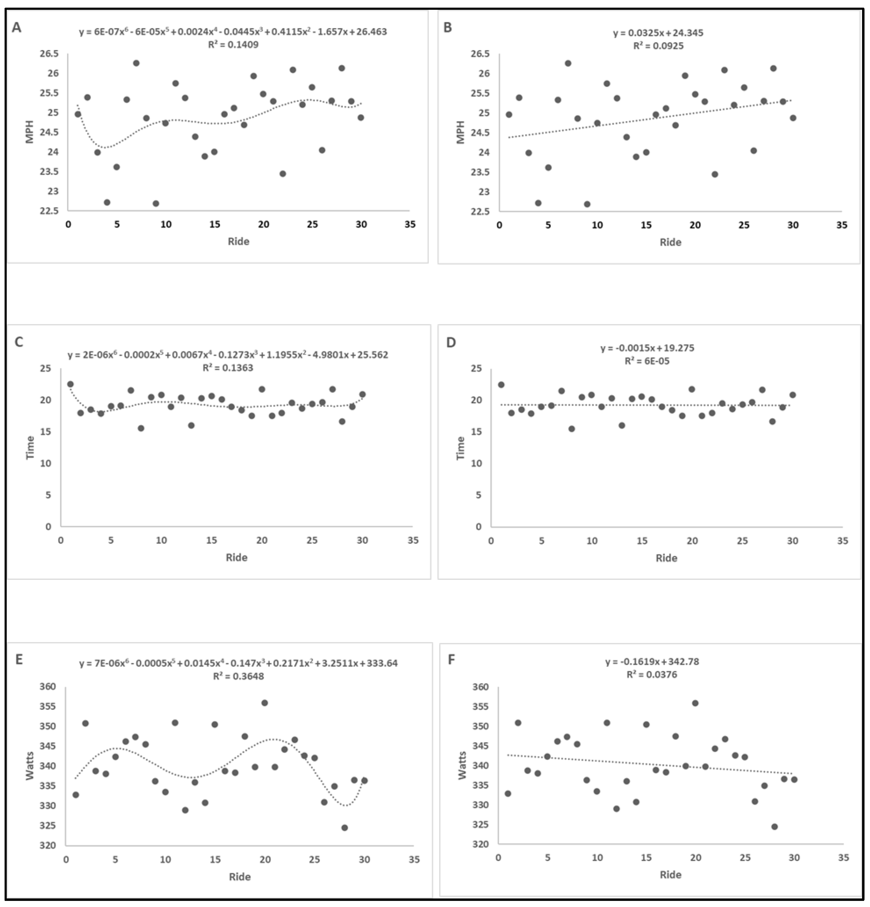
Figure 2.
Sextic polynomial and linear equations for the first cyclist, 100 replications (rides).
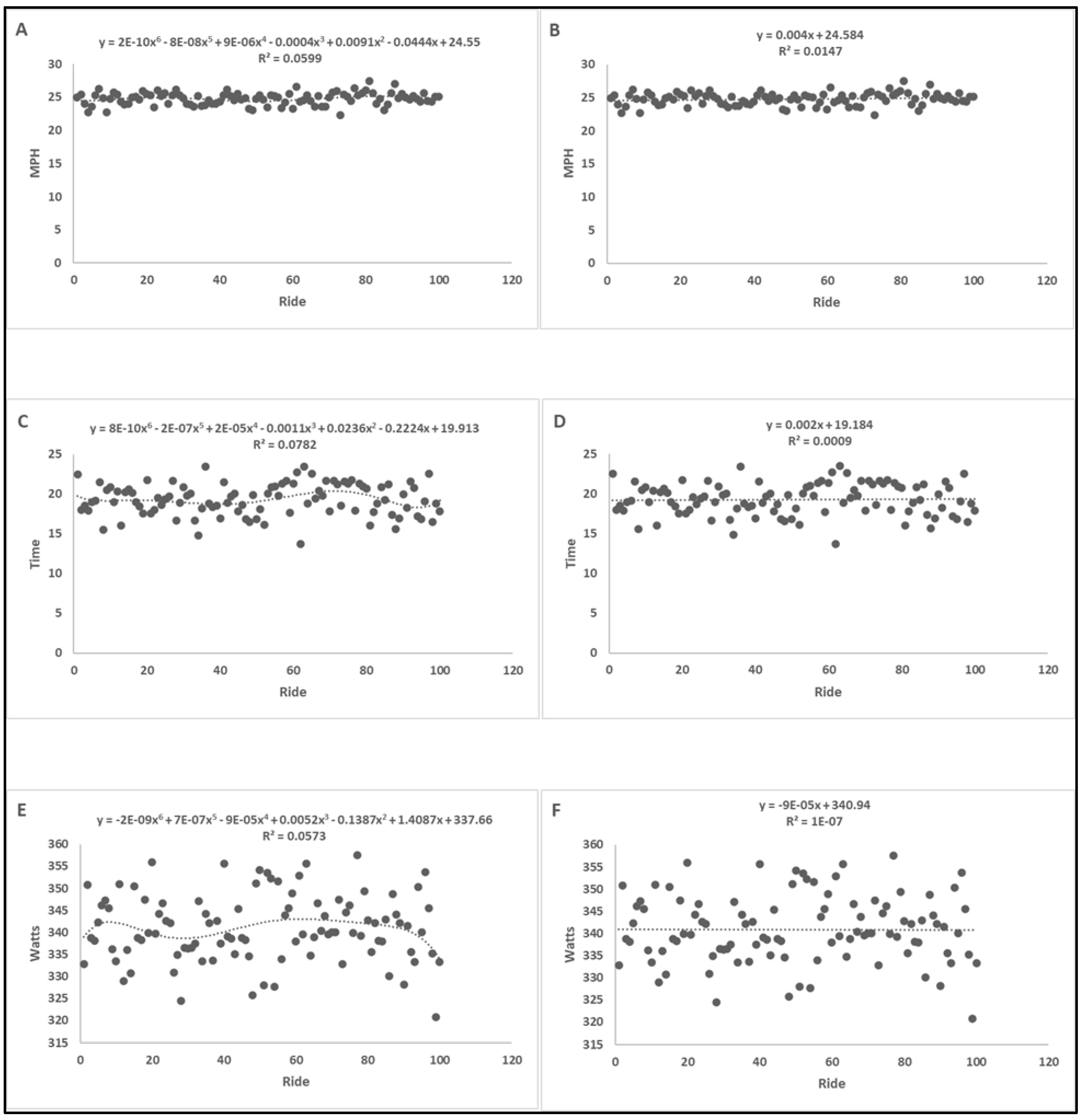
Figure 3.
Mediation model tested.
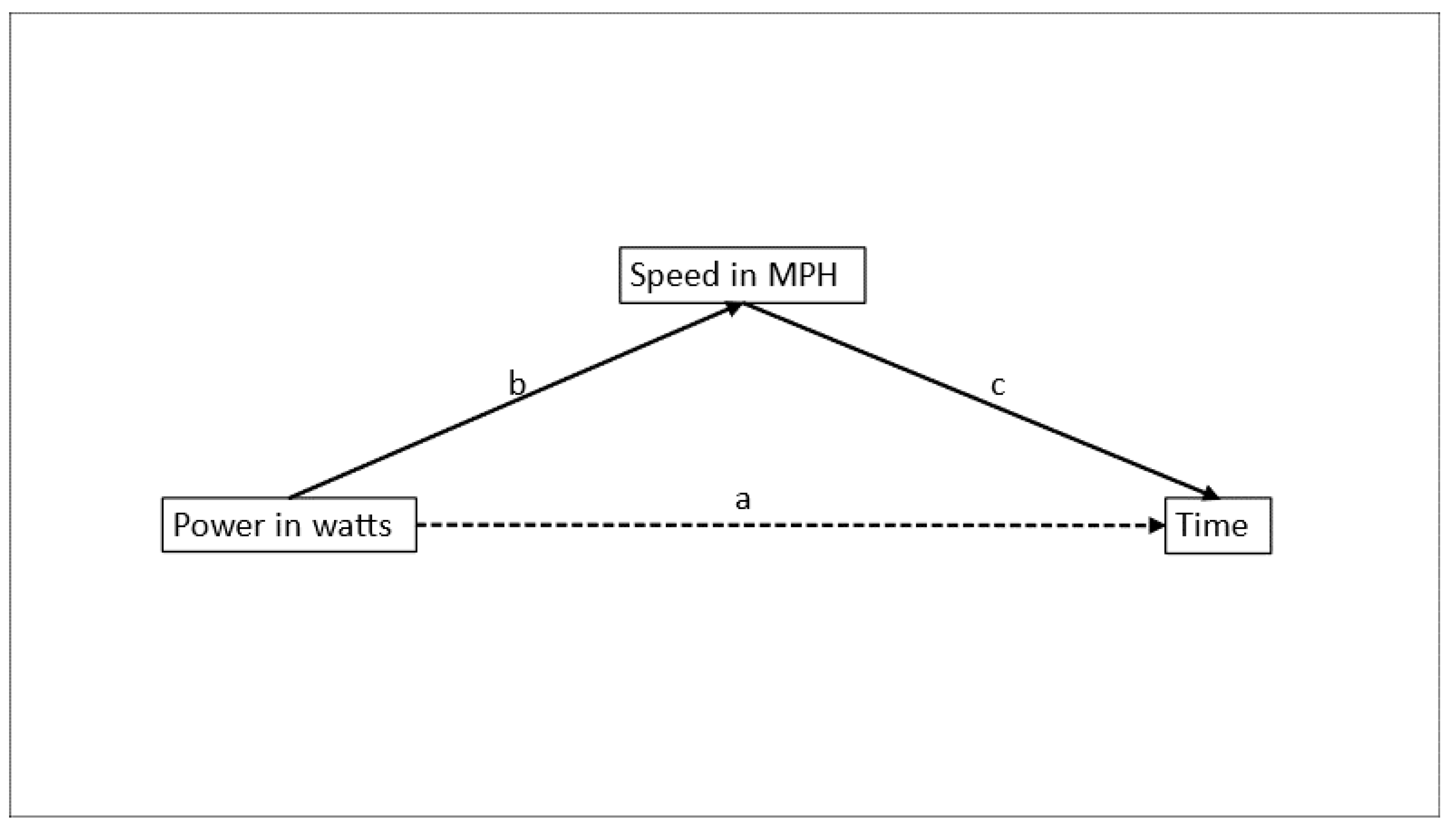
Figure 4.
Residual plots for multiple regression analysis with 30 replications (rides).
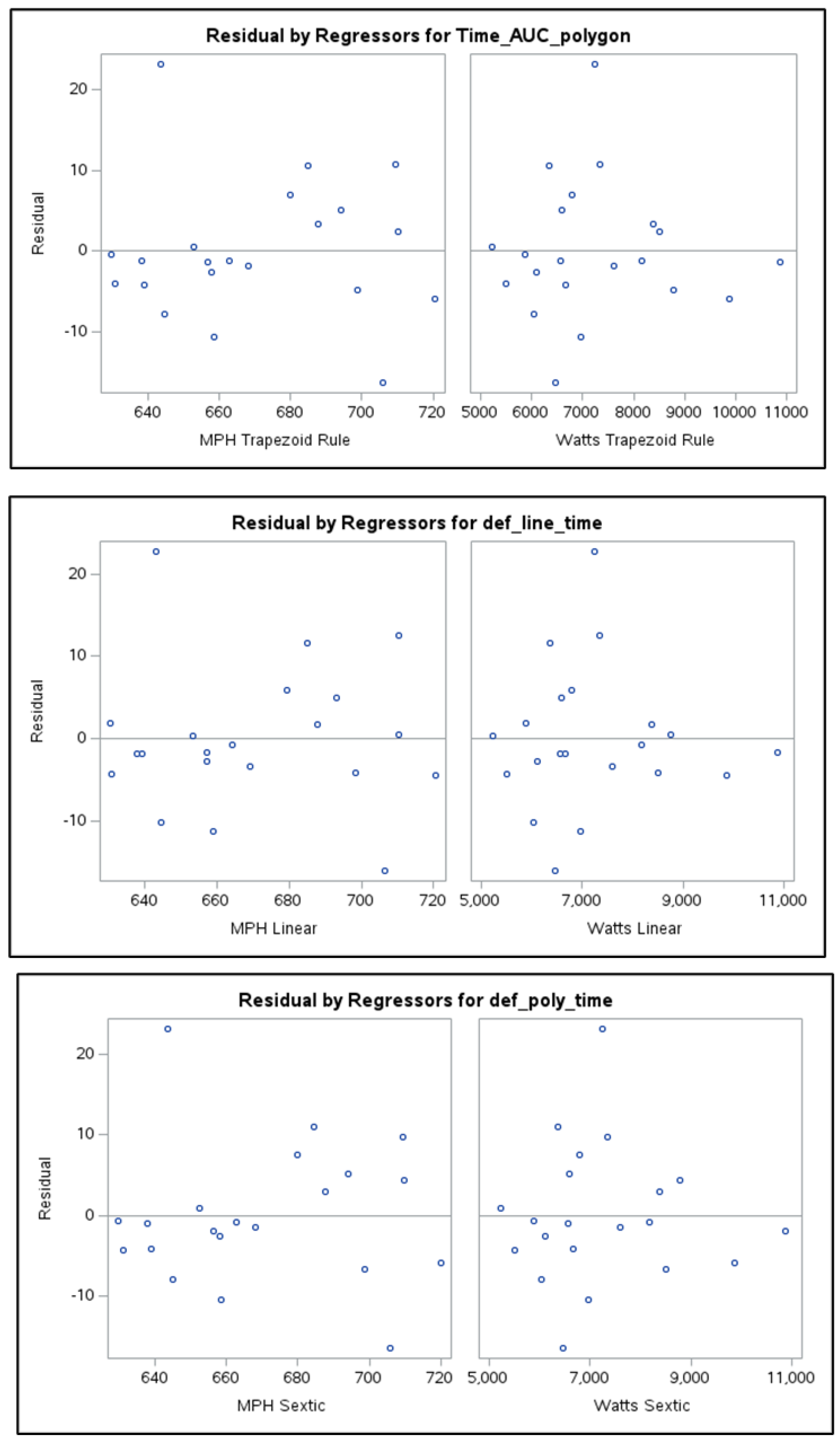
Figure 5.
Residual plots for multiple regression analysis with 100 replications (rides).
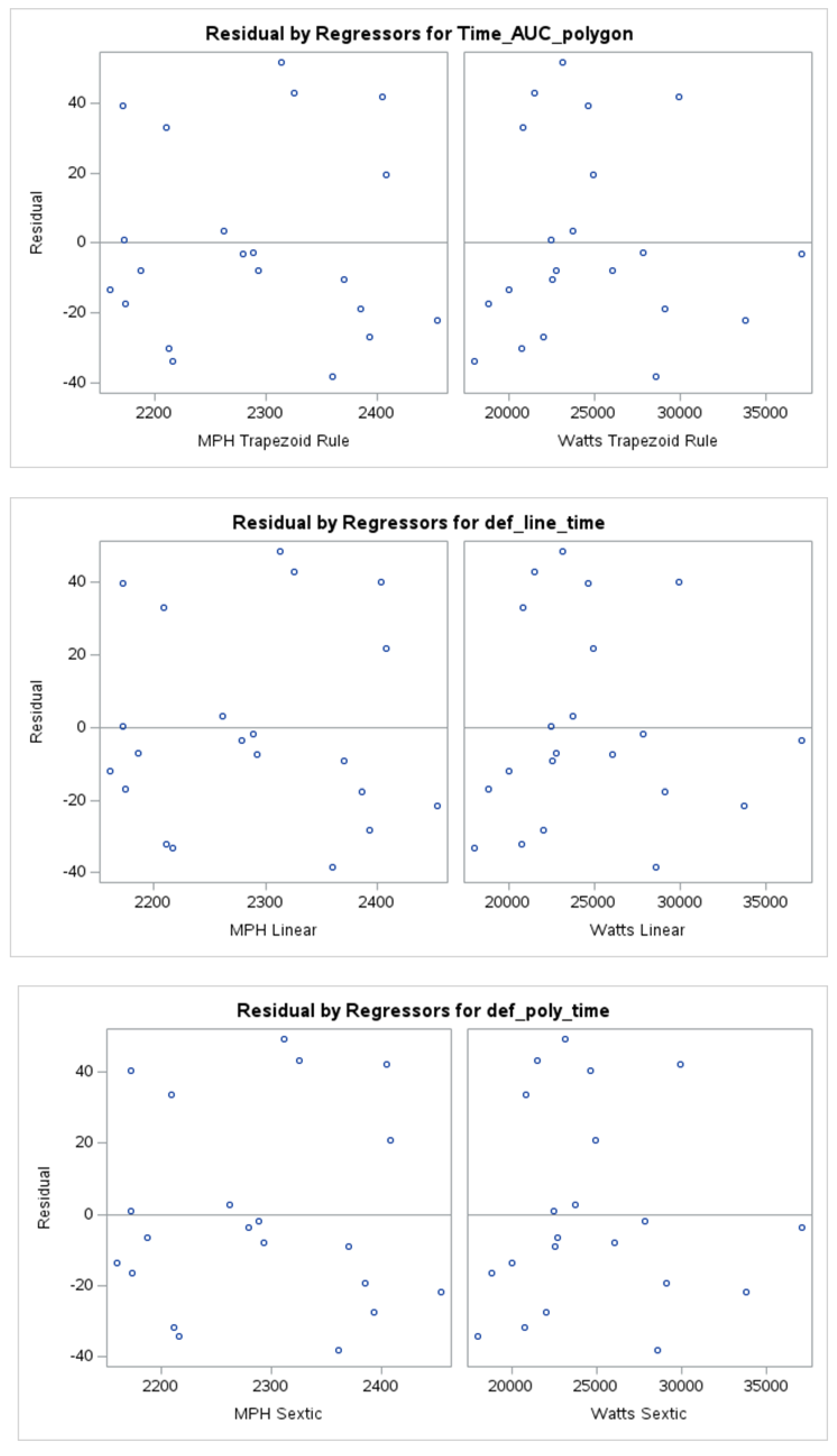

Table 1.
Means, Standard Deviations, Minimums and Maximums for the AUC variables.
| 30 repeated measures (Rides) | |||||
| Variable | Mean | Std Dev | Minimum | Maximum | |
| MPHTrapazoid | 670.180 | 28.609 | 629.638 | 720.533 | |
| MPHlinear | 670.090 | 28.539 | 629.556 | 720.149 | |
| MPHpolynomial | 670.317 | 28.621 | 630.408 | 720.604 | |
| TimeTrapazoid | 612.487 | 27.072 | 555.869 | 656.309 | |
| Timelinear | 612.544 | 27.035 | 556.241 | 656.143 | |
| Timepolynomial | 612.591 | 26.884 | 558.303 | 656.493 | |
| WattsTrapazoid | 7233.000 | 1432.000 | 5223.000 | 10873.000 | |
| Wattslinear | 7232.000 | 1433.000 | 5223.000 | 10876.000 | |
| Wattspolynomial | 7232.000 | 1430.000 | 5226.000 | 10872.000 | |
| 100 repeated measures (Rides) | |||||
| MPHTrapazoid | 2287.000 | 93.138 | 2160.000 | 2454.000 | |
| MPHlinear | 2288.000 | 93.202 | 2161.000 | 2454.000 | |
| MPHpolynomial | 2288.000 | 93.304 | 2160.000 | 2454.000 | |
| TimeTrapazoid | 2094.000 | 90.953 | 1909.000 | 2233.000 | |
| Timelinear | 2094.000 | 90.636 | 1909.000 | 2233.000 | |
| Timepolynomial | 2094.000 | 90.829 | 1909.000 | 2233.000 | |
| WattsTrapazoid | 24693.000 | 4876.000 | 18003.000 | 37065.000 | |
| Wattslinear | 24694.000 | 4874.000 | 18006.000 | 37068.000 | |
| Wattspolynomial | 24693.000 | 4876.000 | 18006.000 | 37072.000 | |
Table 2.
Bivariate correlations among different measurements for AUC for T=30 repeated measures (rides).
Table 2.
Bivariate correlations among different measurements for AUC for T=30 repeated measures (rides).
| MPHTrapazoid | MPHlinear | MPHpolynomial | TimeTrapazoid | Timelinear | Timepolynomial | WattsTrapazoid | Wattslinear | Wattspolynomial | |
| MPHTrapazoid | 1.000 | 0.992*** | 0.992*** | -0.929*** | -0.922*** | -0.929*** | 0.466* | 0.465* | 0.466* |
| MPHlinear | 0.992*** | 1.000 | 1.000*** | -0.930*** | -0.928*** | -0.930*** | 0.471* | 0.471* | 0.471* |
| MPHpolynomial | 0.992*** | 1.000*** | 1.000 | -0.927*** | -0.926*** | -0.927*** | 0.466* | 0.466* | 0.466* |
| TimeTrapazoid | -0.929*** | -0.930*** | -0.927*** | 1.000 | 0.998*** | 1.000*** | -0.616** | -0.615** | -0.615** |
| Timelinear | -0.922*** | -0.928*** | -0.926*** | 0.998*** | 1.000 | 0.998*** | -0.610** | -0.610** | -0.610** |
| Timepolynomial | -0.929*** | -0.930*** | -0.927*** | 1.000*** | 0.998*** | 1.000 | -0.614** | -0.614** | -0.614** |
| WattsTrapazoid | 0.466* | 0.471* | 0.466* | -0.616** | -0.610** | -0.614** | 1.000 | 1.000*** | 1.000*** |
| Wattslinear | 0.465* | 0.471* | 0.466* | -0.615** | -0.610** | -0.614** | 1.000*** | 1.000 | 1.000*** |
| Wattspolynomial | 0.466* | 0.471* | 0.466* | -0.615** | -0.610** | -0.614** | 1.000*** | 1.000*** | 1.000 |
*Significant, p<0.05;**Significant, p<0.01;**Significant, p<0.0001.
Table 3.
Bivariate correlations among different measurements for AUC for T=100 repeated measures (rides).
Table 3.
Bivariate correlations among different measurements for AUC for T=100 repeated measures (rides).
| MPHTrapazoid | MPHlinear | MPHpolynomial | TimeTrapazoid | Timelinear | Timepolynomial | WattsTrapazoid | Wattslinear | Wattspolynomial | |
| MPHTrapazoid | 1.000 | 1.000*** | 1.000*** | -0.948*** | -0.949*** | -0.947*** | 0.549* | 0.549* | 0.548* |
| MPHlinear | 1.000*** | 1.000 | 1.000*** | -0.948*** | -0.949*** | -0.947*** | 0.548* | 0.548* | 0.548* |
| MPHpolynomial | 1.000*** | 1.000*** | 1.000 | -0.948*** | -0.949*** | -0.948*** | 0.549* | 0.549* | 0.549* |
| TimeTrapazoid | -0.948*** | -0.948*** | -0.948*** | 1.000 | 1.000*** | 1.000*** | -0.605** | -0.605** | -0.605** |
| Timelinear | -0.949*** | -0.949*** | -0.949*** | 1.000*** | 1.000 | 1.000*** | -0.603** | -0.603** | -0.603** |
| Timepolynomial | -0.947*** | -0.947*** | -0.948*** | 1.000*** | 1.000*** | 1.000 | -0.604** | -0.604** | -0.604** |
| WattsTrapazoid | 0.549* | 0.548* | 0.549* | -0.605** | -0.603** | -0.604** | 1.000 | 1.000*** | 1.000*** |
| Wattslinear | 0.549* | 0.548* | 0.549* | -0.605** | -0.603** | -0.604** | 1.000*** | 1.000 | 1.000*** |
| Wattspolynomial | 0.548* | 0.548* | 0.549* | -0.605** | -0.603** | -0.604** | 1.000*** | 1.000*** | 1.000 |
*Significant, p<0.05;**Significant, p<0.01;**Significant, p<0.0001.
Table 4.
Simple regression analysis results for the three AUC calculations for T=30 repeated measures (rides).
Table 4.
Simple regression analysis results for the three AUC calculations for T=30 repeated measures (rides).
| 30 repeated measures (Rides) | ||||||||
| Model1 | Variable | Estimate | SE2 | t | p-value | R2 | RMSE3 | |
| 1 | Intercept | 1164.246 | 47.95571 | 24.28 | <.0001 | 0.905 | 8.802 | |
| MPHtrapazoid | -0.77568 | 0.07776 | -9.98 | <.0001 | ||||
| Wattstrapazoid | -0.00441 | 0.00155 | -2.84 | 0.0108 | ||||
| 2 | Intercept | 1161.524 | 48.8195 | 23.79 | <.0001 | 0.90 | 8.95 | |
| MPHlinear | -0.77387 | 0.07924 | -9.77 | <.0001 | ||||
| Wattslinear | -0.00417 | 0.00159 | -2.63 | 0.0169 | ||||
| 3 | Intercept | 1164.183 | 48.69297 | 23.91 | <.0001 | 0.902 | 8.914 | |
| MPHpolynomial | -0.77596 | 0.07895 | -9.83 | <.0001 | ||||
| Wattspolynomial | -0.00438 | 0.00157 | -2.78 | 0.0122 | ||||
| 100 repeated measures (Rides) | ||||||||
| 1 | Intercept | 4119.086 | 171.972 | 23.950 | <.0001 | 0.909 | 28.959 | |
| MPHtrapazoid | -0.861 | 0.083 | -10.350 | <.0001 | ||||
| Wattstrapazoid | -0.002 | 0.002 | -1.420 | 0.172 | ||||
| 2 | Intercept | 4113.517 | 170.100 | 24.180 | <.0001 | 0.91 | 28.678 | |
| MPHlinear | -0.859 | 0.082 | -10.440 | <.0001 | ||||
| Wattslinear | -0.002 | 0.002 | -1.410 | 0.174 | ||||
| 3 | Intercept | 4113.628 | 172.103 | 23.900 | <.0001 | 0.908 | 29.029 | |
| MPHpolynomial | -0.859 | 0.083 | -10.320 | <.0001 | ||||
| Wattspolynomial | -0.002 | 0.002 | -1.400 | 0.180 | ||||
1 Model 1, Trapezoid rule calculation; Model 2, linear model; Model 3, polynomial model; 2Standard Error; 3Root Mean Squared Error.
Table 5.
caption.
| 30 repeated measures (Rides) | |||||||
| Model2 | Effect | Estimate | SE3 | t | p-value | Low | High |
| 1 | Direct | -0.0044 | 0.0016 | -2.8413 | 0.0108 | -0.0077 | -0.0011 |
| Indirect | -0.0072 | -0.0041 | - | - | -0.0162 | -0.0011 | |
| 2 | Direct | -0.0042 | 0.0016 | -2.6319 | 0.0169 | -0.0075 | -0.0008 |
| Indirect | -0.0073 | 0.0042 | - | - | -0.0164 | -0.0012 | |
| 3 | Direct | -0.0044 | 0.0016 | -2.7845 | 0.0122 | -0.0077 | -0.0011 |
| Indirect | -0.0072 | 0.0042 | - | - | -0.0162 | -0.0011 | |
| 100 repeated measures (Rides) | |||||||
| 1 | Direct | -0.0023 | 0.0016 | -1.4221 | 0.1721 | -0.0056 | -0.0023 |
| Indirect | -0.0090 | 0.0038 | - | - | -0.0169 | -0.0032 | |
| 2 | Direct | -0.0022 | 0.0016 | -1.4140 | 0.1744 | -0.0055 | 0.0011 |
| Indirect | -0.0090 | 0.0038 | - | - | -0.0170 | -0.0032 | |
| 3 | Direct | -0.0022 | 0.0016 | -1.3961 | 0.1797 | -0.0056 | 0.0011 |
| Indirect | -0.0090 | 0.0038 | - | - | -0.0170 | -0.0032 | |
1Standard errors and confidence intervals for indirect effects are bootstrapped with 10,000 draws; 2Model 1, Trapezoid rule calculation; Model 2, linear model; Model 3, polynomial model; 3Standard Error.
Disclaimer/Publisher’s Note: The statements, opinions and data contained in all publications are solely those of the individual author(s) and contributor(s) and not of MDPI and/or the editor(s). MDPI and/or the editor(s) disclaim responsibility for any injury to people or property resulting from any ideas, methods, instructions or products referred to in the content. |
© 2026 by the authors. Licensee MDPI, Basel, Switzerland. This article is an open access article distributed under the terms and conditions of the Creative Commons Attribution (CC BY) license (http://creativecommons.org/licenses/by/4.0/).
Copyright: This open access article is published under a Creative Commons CC BY 4.0 license, which permit the free download, distribution, and reuse, provided that the author and preprint are cited in any reuse.


