

Submitted:
16 July 2026
Posted:
17 July 2026
You are already at the latest version
Abstract
This paper examines the determinants of industrial added value in ten major oil-importing economies over the period 1993–2024, with particular attention to the role of oil prices. Using a cross-sectionally augmented autoregressive distributed lag (CS-ARDL) mean group estimator, the study accounts for cross-sectional dependence, heterogeneous dynamics, non-stationarity, and long-run cointegration across countries. The empirical model includes gross fixed capital formation, foreign direct investment, labor force participation, trade openness, consumer price inflation, and the OPEC oil basket price as explanatory variables. The results show that domestic structural factors are the main drivers of industrial performance. In the short run, investment, labor force participation, and trade openness increase industrial value added, while inflation reduces it. In the long run, capital deepening, labor market participation and trade integration remain positively associated with industrial value added, whereas inflation has a negative effect. By contrast, oil prices do not exert a statistically significant direct effect in either the short or long run. These findings suggest that large oil-importing economies have partly adapted to oil-price risk through structural adjustment, greater openness, and macroeconomic stabilization. The evidence implies that industrial policy in such economies should prioritize investment, labor market participation, trade integration, and price stability, while treating oil-price volatility as an external risk rather than a dominant structural constraint.
Keywords:
oil price
; industrial added value
; oil-importing economies
; CS-ARDL
; panel cointegration
; cross-sectional dependence
1. Introduction
Industrial production remains a central engine of economic growth and structural transformation, even as services account for a growing share of global added value. In 2024, industry still represented roughly one quarter of world GDP, reflecting the continued importance of manufacturing, construction, mining, and utilities in employment, innovation, and export performance. Classical macroeconomic models emphasized capital and labor as the main drivers of industrial output, often treating energy—and oil in particular—as a secondary input with limited macroeconomic relevance. The twin oil shocks of the 1970s challenged this view by demonstrating that large and persistent increases in oil prices can trigger recessions, inflationary episodes and major income transfers between oil-importing and oil-exporting countries. Since then, a vast empirical literature has documented that oil-price shocks can affect real activity, inflation, and external balances, with particularly pronounced effects in oil-importing economies.
Over time, however, the relationship between oil prices and industrial activity appears to have become more complex and possibly weaker. Many oil-importing economies have diversified their energy mix, improved energy efficiency, and adopted more credible monetary and fiscal frameworks, which may have reduced their vulnerability to oil-price shocks. Recent studies report heterogeneous and sometimes insignificant effects of oil prices on industrial production, depending on the period, the econometric approach, and the extent to which models account for structural change, cross-country heterogeneity, and global common factors. At the same time, industrial performance in open economies depends strongly on domestic structural conditions such as investment, foreign direct investment (FDI), labor-market participation, trade openness and price stability. These factors shape firms’ capacity to adapt to external cost shocks and to integrate into global value chains.
From an econometric perspective, analyzing the joint role of oil prices and domestic fundamentals in industrial performance poses several challenges. Macroeconomic panel data for country samples typically display strong cross-sectional dependence driven by common shocks, such as global oil-price movements, financial crises, and worldwide demand fluctuations. Standard first-generation panel methods that ignore such dependence can produce biased and inconsistent estimates. Furthermore, the main variables of interest—industrial added value, investment, trade openness and oil prices—are often non-stationary and cointegrated, calling for methods that accommodate mixed integration orders and long-run relationships. In addition, slope coefficients and adjustment speeds are likely heterogeneous across countries that differ in industrial structure, energy intensity, and policy regimes.
This paper addresses these issues by examining the determinants of industrial value added in a panel of ten major oil-importing economies—China, Germany, France, India, Italy, Japan, the Republic of Korea, Spain, South Africa, and Türkiye—over the period 1993–2024. The empirical model relates industrial added value (as a share of GDP) to gross fixed capital formation, FDI, labor force participation, trade openness, consumer price inflation, and the OPEC oil basket price, thereby combining domestic structural drivers with an external energy-price variable in a unified framework. Methodologically, the study employs the cross-sectionally augmented autoregressive distributed lag (CS-ARDL) mean group estimator proposed by Chudik and Pesaran (2015) and further developed by Chudik et al. (2016), which augments country-specific ARDL models with lags of cross-sectional averages of the dependent and explanatory variables. This approach explicitly accounts for strong cross-sectional dependence, non-stationarity, and heterogeneous dynamics, while delivering both short-run and long-run parameter estimates in the presence of cointegration.
The paper makes four contributions to the literature. First, it provides new evidence on the role of oil prices in shaping industrial value added in a relatively large panel of major oil-importing economies, for which the transmission of oil-price shocks may differ from that in oil-exporting or more energy-independent countries. Second, it jointly models external oil-price shocks and key domestic structural determinants—investment, FDI, labor force participation, trade openness, and inflation—within a single empirical framework, thereby assessing the relative importance of external versus internal drivers. Third, it applies a CS-ARDL mean group estimator that explicitly addresses cross-sectional dependence, non-stationarity, and slope heterogeneity and it complements the estimation with second-generation panel unit-root, cointegration, and structural-break tests. Fourth, by contrasting the insignificant direct effect of oil prices with the dominant influence of domestic fundamentals, the paper provides new evidence on how large oil-importing economies have adapted to energy-price risk and on which policy levers are most effective in supporting industrial performance.
The analysis addresses two main questions. First, which factors exert statistically and economically significant short-run and long-run effects on the industrial value-added share of GDP in major oil-importing economies? Second, once domestic fundamentals and common shocks are considered, do oil-price fluctuations still leave a measurable imprint on the level of industrialization? The remainder of the paper is organized as follows. Section 2 reviews the relevant theoretical and empirical literature. Section 3 describes the data and presents descriptive evidence on industrial value-added trends. Section 4 outlines the econometric methodology and preliminary diagnostic tests. Section 5 reports and interprets the CS-ARDL estimation results. Section 6 concludes with a discussion of policy implications and directions for future research.
2. Literature Review
The economic role of oil and energy was long treated as a microeconomic issue, based largely on the availability of a cheap and abundant input. This view changed after the oil crises of 1973–74 and 1979, which exposed the vulnerability of industrial economies to energy-price shocks. Those episodes disrupted growth, generated inflationary pressures, and renewed concern about resource scarcity and long-run economic performance.
Early contributions focused on the macroeconomic transmission of oil-price shocks. Mork (1994) offers a comprehensive review of this literature. Among the pioneering studies, Pierce and Enzler (1974) used a modified version of the MIT-Penn-SSRC (MPS) model and incorporated oil prices into the U.S. money demand equation. Their results suggest that higher oil prices reduce real money balances in importing economies, generating inflationary pressures and recessionary dynamics through monetary channels. In this framework, oil shocks are interpreted primarily as demand-side disturbances.
Another strand of the literature emphasizes income transfers between oil-importing and oil-exporting countries. Fried and Schultze (1975) and Dohner (1981) argue that higher oil prices reduce domestic purchasing power in importing economies, thereby contracting aggregate demand. Mork (1994) shows that these transfers can be quantitatively significant. For example, in the United States, oil-price increases in the 1970s raised the value of oil imports by around 2 percent of GDP.
Subsequent research shifted attention toward supply-side effects. Rasche and Tatom (1977a, b) modeled output using an aggregate production function that includes energy as an input. They show that increases in energy prices reduce potential output by raising production costs. However, this approach has been criticized for possible inconsistencies with national accounting frameworks, particularly the double-deflation issue (Mork, 1995).
Hamilton (1983) marked a major shift by analyzing oil shocks within a real business cycle framework. Using Granger causality techniques, he showed that oil-price increases precede most U.S. recessions in the postwar period. In this setting, oil shocks are treated as exogenous supply disturbances that affect production decisions, labor demand, and investment.
Later studies extended the analysis to international settings. Burbidge and Harrison (1984) find that oil-price increases reduce industrial production across major advanced economies, with stronger effects in oil-importing countries. Mork (1989) introduces asymmetry, showing that oil-price increases have significant negative effects, whereas price decreases generate only limited positive responses. Hooker (1996) documents a structural break in the oil–output relationship after the mid-1980s and attributes it to improved energy efficiency and changes in monetary policy.
During the 2000s, the literature moved toward more advanced econometric frameworks. Researchers increasingly used cointegration techniques and nonlinear models to capture long-run relationships and asymmetries. Papapetrou (2001) finds that oil-price increases reduce industrial production and employment in Greece using a VAR model. Jiménez-Rodríguez and Sánchez (2005) extend the analysis to OECD countries and show that the effects vary across economies depending on energy intensity. Lardic and Mignon (2006) apply an asymmetric cointegration approach and confirm that oil-price increases have stronger negative effects than price decreases.
More recent studies decompose oil-price movements into different types of shocks. Kilian and Vigfusson (2011) and Baumeister and Peersman (2013) distinguish supply-driven, demand-driven, and risk-driven shocks. They show that supply-side shocks have the most persistent negative effects on output in oil-importing economies. By contrast, demand-driven oil-price increases often coincide with global economic expansions, which partly offset their adverse impact.
Recent empirical evidence suggests that the effect of oil prices on industrial activity has weakened over time. This trend reflects energy diversification, efficiency gains, and more credible monetary policy frameworks. Kalymbetova et al. (2021), using panel cointegration methods, find a positive long-run relationship between oil prices and industrial production in a sample of oil-importing countries. Their result suggests that some economies have adapted to higher energy costs through technological upgrading and structural transformation.
In contrast, Rahmouni and Al Kahtani (2025) employ a panel ARDL (PMG) approach for G20 economies over 1979–2020. They find that oil prices have a negligible effect in the short run and a weak negative effect in the long run. This indicates that while immediate responses are limited, persistent oil-price increases may still constrain industrial performance.
Finally, recent micro-level evidence from Gomes et al. (2025) examine the impact of oil shocks on labor markets. The study shows that oil supply shocks lead to significant and persistent declines in employment and production in oil-intensive sectors of importing economies. These findings reinforce the contractionary effects associated with adverse oil shocks.
Overall, the empirical literature provides mixed evidence on the role of oil prices in shaping industrial activity. Early studies emphasize strong and predominantly negative effects, whereas more recent contributions point to weaker, more heterogeneous, and sometimes insignificant impacts. These differences reflect variations in econometric approaches, sample periods, and the extent to which studies account for structural change, cross-country heterogeneity, and global common factors. Moreover, relatively few studies jointly examine oil prices alongside key domestic determinants of industrial value added within a unified empirical framework. This leaves an important gap concerning the relative importance of external energy shocks versus internal structural drivers. The present study addresses this gap by employing a CS-ARDL approach that explicitly accounts for cross-sectional dependence, heterogeneous dynamics, and long-run relationships, thereby providing more robust evidence on the determinants of industrial performance in oil-importing economies.
3. Data and Methodology
3.1. Data Sources and Variable Definition
The analysis uses annual panel data for ten major oil-importing economies over the period 1993–2024. The sample includes China, Germany, France, India, Italy, Japan, the Republic of Korea, Spain, South Africa, and Türkiye. These countries differ in their stages of industrialization, energy policy frameworks, and macroeconomic conditions.
The dependent variable is industrial added value as a percentage of GDP (IAV), obtained from the World Bank’s World Development Indicators (WDI). Industrial added value includes manufacturing, mining, construction, and utilities, while excluding agriculture and services. This indicator captures the industrial sector’s contribution to total output and is widely used in studies of structural transformation.
The independent variables include:
Foreign direct investment, net inflows as a percentage of GDP (FDI), sourced from WDI. FDI captures external capital flows and technology transfer that may affect industrial capacity.
Gross fixed capital formation as a percentage of GDP (GFCF), sourced from WDI. GFCF measures domestic investment in physical capital and infrastructure.
Labor force participation rate, total (percentage of total population ages 15+) (LFP), sourced from WDI. LFP reflects the availability of labor for industrial production.
Trade as a percentage of GDP (Trade), defined as the sum of exports and imports of goods and services, sourced from WDI. Trade openness captures the degree of integration with global markets and exposure to international competition.
Consumer price index (CPI, 2010=100), sourced from WDI. CPI reflects domestic inflation and the stability of the macroeconomic environment.
Crude oil price, OPEC Basket (OP, US dollars per barrel), sourced from the Organization of Petroleum Exporting Countries (OPEC).
3.2. Descriptive Statistics
Table 1 reports the descriptive statistics for the main variables. The summary statistics show considerable variation across the panel, especially for CPI, OP, and trade openness, which suggests substantial heterogeneity among the selected economies. This variation supports the use of an econometric framework that allows for country-specific dynamics rather than imposing a fully homogeneous structure.
3.3. Trends in Industrial Added Value
Figure 1 suggests that the evolution of industrial value added over 1993–2024 is driven primarily by structural transformation rather than by short-run cyclical movements, with oil prices playing a reinforcing but not determining role. In advanced European economies (France, Italy and Spain) as well as in Japan, the persistent decline in IAV reflects a mature stage of development characterized by deindustrialization, a reallocation of resources toward high-value-added services, and an international fragmentation of production. The apparent break around the Global Financial Crisis points not only to a cyclical disturbance but also to a more lasting shift in industrial capacity, after which manufacturing stabilizes at a lower equilibrium share.
By contrast, Korea displays a more resilient industrial structure, as reflected in the relative stability of IAV. This pattern suggests stronger integration of manufacturing into global value chains and a greater ability to absorb energy-price shocks. Among emerging economies, the trajectories are more diverse and reflect different stages of structural change. China’s high but gradually declining IAV indicates a managed transition toward more sophisticated and less energy-intensive production, along with diminishing sensitivity to oil-price fluctuations. India’s inverted U-shaped pattern points to a more constrained industrialization process, in which the post-2008 decline reflects both structural bottlenecks and greater exposure to rising energy costs. Turkey’s pronounced volatility highlights the macroeconomic vulnerability associated with heavy dependence on imported energy, as oil-price shocks are transmitted rapidly into industrial fluctuations. In contrast, South Africa’s smoother downward trend suggests a more gradual and less oil-sensitive process of structural adjustment.
Taken together, these patterns point to a form of conditional convergence in industrial shares, in which countries with different initial conditions tend to move toward lower IAV levels as development advances. However, the speed, the volatility, and the transitional dynamics of this adjustment are shaped by energy dependence and exposure to oil-price shocks. In this sense, oil prices appear less as a fundamental driver of structural change than as a transmission channel that amplifies short-run deviations around a long-run transformation path shaped by technological progress, globalization, and sectoral reallocation.
4. The Econometric Methodology and Preliminary Tests
4.1. Econometric Methodology
The availability of panel data, particularly at the country level, has encouraged the use of econometric methods that exploit both the cross-sectional and time-series dimensions of the data. In this context, the pioneering work of Pesaran and Smith (1995) and Pesaran, Shin, and Smith (1999) emphasized the importance of allowing slope heterogeneity across cross-sectional units. Pesaran and Smith (1995) proposed the Mean Group (MG) estimator, which provides consistent estimates of average long-run parameters by estimating separate regressions for each cross-sectional unit and then averaging the coefficients. This approach differs from conventional pooled estimators, such as fixed effects and random effects models, which typically impose homogeneity on slope coefficients. Pesaran, Shin, and Smith (1999) later introduced the Pooled Mean Group (PMG) estimator, which allows heterogeneity in short-run dynamics and error variances while imposing homogeneity on the long-run coefficients.
A further limitation of early panel estimators is that they often ignore unobserved common factors and cross-sectional dependence. The estimated equation can be written as follows:
where is the vector of unobserved common factors, denotes heterogeneous factor loadings, and represents the unit-specific fixed effect. The term denotes the individual-specific idiosyncratic error, assumed to be independently distributed from . The heterogeneous slope coefficients are randomly distributed, such that , where is IID with variance-covariance matrix .
Pesaran (2006) addressed this issue by proposing the Common Correlated Effects (CCE) estimator, which approximates latent common factors using cross-sectional averages of the explanatory variables. In dynamic panels, however, the presence of a lagged dependent variable creates additional complications because the standard CCE estimator may become inconsistent when regressors are not strictly exogenous. To address this problem, Chudik and Pesaran (2015) proposed augmenting the model with a sufficient number of lags of cross-sectional averages. This yields a dynamic specification that remains consistent under cross-sectional dependence and can be written as:
where . If , then the MG estimates are obtained as:
Building on this framework and using an error-correction representation, Chudik et al. (2016) propose the Cross-Sectionally Augmented ARDL (CS-ARDL) model with the Mean Group (MG) estimator:
Where:
is the error-correction coefficient and is expected to be negative. The long-run coefficients are estimated by maximum likelihood estimator, whereas the short-run coefficients are estimated by OLS one.
4.2. Cross-Sectional Dependence
Before estimating the model, it is necessary to test for cross-sectional dependence. In macroeconomic panels, countries are often exposed to common shocks such as oil-price movements, financial crises, and global demand fluctuations. Ignoring such dependence may lead to biased and inconsistent estimates. Pesaran (2015) proposes the CD test to detect cross-sectional dependence in panel residuals and variables. Rejection of the null hypothesis of cross-sectional independence suggests that common factors are present and should be explicitly modeled. The test statistic is calculated as:
where the correlation coefficient is calculated:
Table 2 shows that the null hypothesis is rejected for all variables except GFCF. Thus, GFCF appears weakly dependent, while the remaining variables exhibit strong cross-sectional dependence. This result confirms the presence of common shocks across the panel and justifies the use of second-generation estimators.
In latent-factor or CCE-type models, Pesaran and Xie (2021) introduced the CD* test, a bias-corrected version of the CD statistic that adjusts analytically for the effect of factor structures. In addition, the degree of cross-sectional dependence can be summarized by the exponent . Dependence is classified as weak when , semi-weak when , and strong when . Bailey et al. (2019) developed a consistent estimator of in panel settings. As presented in Table 3, the CD and CD* residual-based tests, together with the estimated value of , confirm that common shocks are present in the data and must be accounted for in the empirical model.
4.3. Panel Unit Root Tests
Since the ARDL framework is designed for variables integrated of order zero or one, the order of integration must be verified before estimation. Given the presence of cross-sectional dependence, second-generation panel unit root tests are more appropriate than first-generation tests. Moreover, as the panel is unbalanced, the CIPS test of Pesaran (2007) is used to examine whether the variables are stationary at levels or in first differences. This test augments standard the Dickey-fuller (ADF) regressions with cross-sectional averages, thereby accounting for common shocks across countries. The test consists to regress the following equation:
Where, the null hypothesis is for all i (homogenous non-stationary), against the possibly heterogenous alternatives for some panels: ,
Table 4 reports the CIPS results at levels and first differences. All variables are non-stationary in levels and stationary in first differences, confirming that they are integrated of order one, I(1).
4.4. Cointegration Tests
To test for a long-run relationship among the model variables, the literature distinguishes between residual-based and error-correction-based approaches. Residual-based tests, such as the Engle and Granger (1987) procedure, examine whether the residuals from the estimated relationship are stationary. In panel settings, Kao (1999) and Pedroni (2004) proposed first-generation residual-based tests. These tests rely on the assumption of cross-sectional independence and are therefore less suitable when common shocks affect all units.
By contrast, error-correction-based tests provide a more flexible framework. Westerlund (2007) proposes panel cointegration tests based on the error-correction representation. These tests allow for heterogeneity across cross-sectional units and can accommodate cross-sectional dependence through bootstrap procedures. The Westerlund framework includes four statistics: and , which test whether cointegration holds for at least one cross-sectional unit, and and , which test whether cointegration holds for the panel as a whole. In this study, these tests are used to assess whether the variables share a stable long-run equilibrium relationship.
Table 5 shows that the panel statistics and clearly reject the null hypothesis of no cointegration, providing robust evidence of a long-run equilibrium relationship among the variables at the panel level. By contrast, the group-level statistics are weaker: does not reject the null, whereas , using the robust p-value, suggests that cointegration holds for at least some, though not necessarily all, cross-sectional units. Persyn and Westerlund (2008) note that in panels with a relatively small time-series dimension ( in our study), the results may be more sensitive and may no longer reject the null. Overall, the pattern of results supports the presence of panel cointegration and justifies the use of long-run and error-correction specifications.
4.5. Slope Homogeneity Tests
Slope homogeneity is tested using the standardized procedure developed by Pesaran and Yamagata (2008), which extends Swamy’s (1970) framework. The Delta test compares a restricted model that imposes slope homogeneity with an unrestricted model that allows coefficients to vary across cross-sectional units. The test is robust to non-normally distributed errors and can be extended to settings with serial correlation. Westerlund (2013) later proposed a heteroskedasticity- and autocorrelation-consistent version of the test statistic. More recently, Bersvendsen and Ditzen (2020) introduced an alternative variant based on simulation methods, which improves robustness in the presence of cross-sectional dependence by augmenting the test with cross-sectional averages.
As shown in Table 6, the test rejects the null hypothesis of homogeneous slope coefficients, as evidenced by the significant Delta statistic (4.444, p = 0.000) and adjusted Delta statistic (5.410, p = 0.000). This confirms that the relationship between the dependent variable and the explanatory variables varies across cross-sectional units and highlights substantial slope heterogeneity in the panel. Consequently, subsequent estimation should explicitly account for cross-sectional heterogeneity.
4.6. Presence of Structural Breaks
To examine whether the sample period contains regime shifts, this study applies the panel structural break test developed by Ditzen, Karavias, and Westerlund (2025), building on the Bai and Perron (1998, 2003) framework. Unlike traditional time-series break tests, this approach is designed for panel data and remains valid in the presence of cross-sectional dependence. The method allows for both known and unknown break dates. Here, we consider the case in which break dates are unknown and test the null hypothesis of no break against the alternative of multiple breaks.
As shown in Table 7, the test indicates that the null hypothesis of no structural breaks cannot be rejected, even though the procedure identifies three potential break dates (2000, 2008, and 2014). The supF statistic equals 1.36, which is substantially below the critical values at the 10%, 5%, and 1% significance levels (6.09, 6.84, and 8.42, respectively). This implies that there is no statistically significant evidence of multiple structural breaks in the estimated relationship. Accordingly, the estimated break dates should be interpreted as algorithm-driven suggestions rather than formally validated structural shifts. The specification without structural breaks therefore remains the preferred model.
The preliminary diagnostic tests jointly confirm the appropriateness of the econometric framework adopted in this study. The cross-sectional dependence tests indicate that the panel is affected by strong common shocks, rendering estimation methods that ignore interdependence across units inappropriate. The panel unit root tests show that all variables are integrated of order one, supporting the use of panel cointegration methods and the CS-ARDL specification. The Westerlund cointegration tests confirm the existence of a long-run equilibrium relationship among the variables, while the slope homogeneity test rejects parameter homogeneity and reveals substantial heterogeneity across countries. Finally, the structural break test does not detect statistically significant regime shifts over the sample period, suggesting a stable underlying relationship. Collectively, these results validate the CS-ARDL Mean Group (MG) approach and provide a sound basis for the estimation outcomes reported in the subsequent tables.
5. Estimation results
The paper examines the determinants of industrial value added in a panel of ten major oil-importing economies over 1993–2024 using the following specification in equation (9):
Estimation results from the CS-ARDL Mean Group (MG) approach proposed by Chudik et al. (2016) are reported in Table 8 and Table 9 for the short run and long run, respectively.
As shown in Table 8, in the short run, investment, labor participation, trade openness, and inflation all exert economically meaningful effects on IAV. In this panel of ten large oil-importing countries, higher GFCF reflects greater investment in machinery, infrastructure, and productive capital, which quickly expands industrial production capacity. Accordingly, a 1 percentage-point increase in the investment share of GDP raises the industrial value-added share by about 0.15 percentage points, as new capital is deployed in manufacturing and related activities.
A higher labor force participation rate also supports industrial activity by expanding the pool of available workers, easing labor-supply constraints, and allowing firms to scale up production. A 1 percentage-point increase in labor force participation is associated with an increase of roughly 0.26 percentage points in the industrial share. Likewise, greater trade openness promotes integration into global value chains, export opportunities, and access to imported intermediate inputs and technology, all of which support industrial output. A 1 percentage-point increase in trade-to-GDP is therefore associated with a rise of about 0.09 percentage points in industrial added value.
By contrast, higher inflation erodes real purchasing power, raises input costs such as wages and imported intermediates, and creates uncertainty that weakens industrial margins. As a result, a 1 percentage-point increase in CPI lowers the industrial share by about 0.10 percentage points. Finally, the lack of a statistically significant short-run effect of oil prices suggests that, in these diversified oil-importing economies, firms and households can absorb temporary oil-price movements through pricing adjustments, substitution, or policy responses. Short-run fluctuations in the nominal OPEC basket price therefore do not translate immediately into measurable changes in the industrial share of GDP.
This finding indicates that oil-price changes operate mainly as external cost and competitiveness shocks, but their short-run channel is weaker than domestic structural drivers of IAV. In the regression, a one-dollar change in the nominal OPEC basket price does not have a statistically significant contemporaneous effect on the industrial share. Instead, domestic investment, labor participation, and trade openness drive short-run industrial dynamics. This implies that firms and policymakers in these economies are able to partially buffer temporary oil-price swings through pricing adjustments, substitution toward more efficient technologies, energy taxes, subsidies, and macroeconomic policy. Oil-price volatility therefore appears to affect industrial added value basically through indirect and slower channels, such as inflation, real income, and external balances, which are partly captured by CPI and trade openness.
In the long run, Table 9 shows that domestic structural factors continue to dominate the determination of the industrial added value share in these oil-importing economies. By contrast, oil-price fluctuations do not leave a statistically detectable permanent imprint on that share. A permanent 1 percentage-point increase in GFCF raises industrial value added by about 0.23 percentage points, indicating that sustained capital deepening in machinery, infrastructure, and productive equipment translates into a lasting expansion of the industrial sector’s weight in GDP.
Similarly, a 1 percentage-point rise in labor force participation is associated with a 0.55 percentage-point long-run increase in industrial value added. This result suggests that a persistently larger and more engaged workforce supports a more industrially oriented production structure. Greater long-run trade openness also reinforces industrialization, a 1 percentage-point increase in trade-to-GDP raises industrial value added by about 0.19 percentage points. This outcome is consistent with the view that sustained integration into global markets, supply chains, and technology flows anchors a higher industrial share.
In contrast, a 1 percentage-point permanent increase in CPI reduces IAV by roughly 0.21 percentage points, suggesting that chronic inflation undermines industrial competitiveness by eroding real demand and raising input costs. The insignificant long-run coefficient on oil prices indicates that, across the panel, the industrial share adjusts over time so that persistent changes in the nominal OPEC basket price do not systematically affect the long-run share of GDP generated by industry. Energy-price shocks are gradually absorbed through efficiency gains, substitution, and policy responses. Whereas the enduring structure of industry is mainly determined by investment, labor, openness, and macroeconomic stability.
The findings imply that policymakers in large oil-importing economies should prioritize measures that strengthen productive investment, labor-force participation, trade openness, and macroeconomic stability, while treating oil-price volatility as a manageable external risk. First, both public and private investment should be expanded in industrial infrastructure, logistics, and digital technologies. Policy support can be delivered through tax incentives, credit guarantees, and development bank financing, which help channel capital toward manufacturing, tradable services, and energy-efficient technologies.
Second, labor-market reforms are needed to reduce barriers for women, youth, and older workers. Expanding upskilling programs is equally important to ensure that higher labor-force participation translates into productive industrial employment. Third, deeper trade integration can support industrial development through trade agreements, better trade infrastructure, and lower non-tariff barriers. These measures help firms access export opportunities, imported intermediate inputs, and technology transfer.
Fourth, price stability should be preserved through credible and forward-looking monetary policy, coordinated with fiscal and wage-setting frameworks to prevent persistent cost-push inflation that undermines industrial competitiveness. In parallel, oil-price shocks should be treated as external cost and competitiveness disturbances whose effects can be mitigated through diversification of the energy mix, strategic reserves, and hedging or stabilization mechanisms to smooth impacts on fiscal balances and external accounts. Finally, industrial and energy strategies should be grounded in empirical frameworks that account for cross-country heterogeneity, cross-sectional dependence, and cointegration, such as the CS-ARDL approach, and should be updated regularly to reflect changes in technology, sectoral structure, and policy regimes.
6. Conclusion and Policy Implications
This paper examines the determinants of industrial added value in ten major oil-importing economies over the period 1993–2024 using a CS-ARDL Mean Group framework that accounts for cross-sectional dependence, integrated variables, and panel cointegration. The results show that IAV is primarily driven by domestic investment, labor force participation, trade openness, and inflation, while oil prices do not have a statistically significant direct effect once these factors and common shocks are controlled for.
In the short run, higher capital formation, stronger labor force participation, and greater trade integration increase IAV, whereas higher inflation reduces it. Oil-price changes are largely absorbed through pricing adjustments, substitution effects, and policy responses. In the long run, sustained capital deepening, a larger workforce, and continued trade openness support industrial expansion, while persistent inflation weakens industrial competitiveness. The oil-price coefficient remains insignificant in both horizons.
These findings suggest that large oil-importing economies have adapted to oil-price volatility through efficiency gains, diversification and macroeconomic reforms. As a result, industrial performance depends more on domestic fundamentals than on external oil-market conditions. From a policy perspective, industrialization strategies should therefore prioritize investment, labor-market participation, trade integration, and price stability, while complementary energy and macroprudential policies manage oil-price risk indirectly rather than attempting to neutralize it.
In the current environment of heightened geopolitical tensions, including those involving Iran and the United States, oil markets may remain exposed to short-term volatility and external imbalances. However, the empirical results indicate that the long-run effects on industrial performance are likely to remain limited as long as domestic policies remain sound. These developments nonetheless underscore the importance of energy diversification and resilient policy frameworks.
Future research could extend this analysis to sector-level data and alternative energy prices and incorporate post-2024 developments. Such extensions would help assess whether energy transitions and geopolitical shocks are reshaping the relationship between oil prices and industrial performance in oil-importing economies.
Funding
This research received no external funding.
Data Availability Statement
The data used in this study are publicly available in the World Bank Data (https://databank.worldbank.org/source/world-development-indicators, accessed on June 2025), and OPEC basket price (https://www.opec.org/opec-basket-price.html, accessed on June 2025).
Conflicts of Interest
The authors declare no conflicts of interest.
Abbreviations
The following abbreviations are used in this manuscript:
| CS-ARDL | Cross-sectionally augmented autoregressive distributed lag (CS-ARDL) |
| OPEC | Organization of the Petroleum Exporting countries |
| VAR | Vector Autoregression |
References
- Bai, J.; Perron, P. Estimating and Testing Linear Models with Multiple Structural Changes. Econometrica 1998, 66(1), 47–78. Available online: https://www.jstor.org/stable/2998540. [CrossRef]
- Bai, J.; Perron, P. Computation and analysis of multiple structural change models. Journal of Applied Econometrics 2003, 18(1), 1–22. [Google Scholar] [CrossRef]
- Bailey, N.; Kapetanios, G.; Pesaran, M. H. Exponent of cross-sectional dependence: Estimation and inference. Journal of Applied Econometrics 2016, 31(6), 929–960. [Google Scholar]
- Bailey, N.; Kapetanios, G.; Pesaran, M.H. Exponent of Cross-sectional Dependence for Residuals. Sankhya B 2019, 81 (Suppl 1), 46–102. [Google Scholar] [CrossRef]
- Baumeister, C.; Peersman, G. Time-varying effects of oil supply shocks on the U.S. economy. American Economic Journal: Macroeconomics 2013, 5(4), 1–28. [Google Scholar] [CrossRef]
- Bersvendsen, T.; Ditzen, J. Testing for slope heterogeneity in Stata. The Stata Journal 2021, 21(1), 51–80. [Google Scholar] [CrossRef]
- Blomquist, J.; Westerlund, J. Testing slope homogeneity in large panels with serial correlation. Economics Letters 2013, 121(3), 374–378. [Google Scholar] [CrossRef]
- Burbidge, J.; Harrison, A. Testing for the effects of oil-price rises using vector autoregressions. International Economic Review 1984, 25(2), 459–484. [Google Scholar] [CrossRef]
- Chudik, A.; Mohaddes, K.; Pesaran, M. H.; Raissi, M. Long-run effects in large heterogeneous panel data models with cross-sectionally correlated errors. In Essays in Honor of Aman Ullah (Advances in Econometrics, Vol. 36, pp. 85-135); Gonzalez-Rivera, G., Hill, R. C., Lee, T.-H., Eds.; Emerald Group Publishing Limited, 2016. [Google Scholar] [CrossRef]
- Chudik, A.; Pesaran, M. H. Common correlated effects estimation of heterogeneous dynamic panel data models with weakly exogenous regressors. Journal of Econometrics 2015, 188(2), 393–420. [Google Scholar] [CrossRef]
- Ditzen, J.; Karavias, Y.; Westerlund, J. Testing and estimating structural breaks in time series and panel data in Stata. The Stata Journal: Promoting Communications on Statistics and Stata 2025, 25(3), 526–560. [Google Scholar] [CrossRef]
- Dohner, Robert S. Energy Prices, Economic Activity, and Inflation: Survey of Issues and Results. In Energy Prices, Inflation, and Economic Activity; Mork, Knut Anton, Ed.; Ballinger: Cambridge, Mass., 1981. [Google Scholar]
- Engle, R. F.; Granger, C. W. J. Co-integration and error correction: Representation, estimation, and testing. Econometrica 1987, 55(2), 251–276. [Google Scholar] [CrossRef]
- Fried, E. R.; Schultze, C. L. Overview. In Higher oil prices and the world economy: The adjustment problem; Fried, E. R., Schultze, C. L., Eds.; The Brookings Institution, 1975; pp. 1–16. [Google Scholar]
- Gomes, D. B. P.; Kolovich, L. L.; Wei, H. Y. Oil Shocks and Labor Market Developments (IMF Working Paper No. 2025/145); International Monetary Fund, 2025. [Google Scholar] [CrossRef]
- Hamilton, J. D. Oil and the macroeconomy since World War II. Journal of Political Economy 1983, 91(2), 228–248. [Google Scholar] [CrossRef]
- Hooker, M. A. What happened to the oil price–macroeconomy relationship? Journal of Monetary Economics 1996, 38(2), 195–213. [Google Scholar] [CrossRef]
- Jiménez-Rodríguez, R.; Sánchez, M. Oil price shocks and real GDP growth: Empirical evidence for some OECD countries. Applied Economics 2005, 37(2), 201–228. [Google Scholar] [CrossRef]
- Kalymbetova, A.; Zhetibayev, Z.; Kambar, R.; Ranov, Z.; Izatullayeva, B. The Effect of Oil Prices on Industrial Production in Oil-importing Countries: Panel Cointegration Test. International Journal of Energy Economics and Policy 2020, 11(1), 186–192. [Google Scholar] [CrossRef]
- Kao, C. Spurious regression and residual-based tests for cointegration in panel data. Journal of Econometrics 1999, 90(1), 1–44. [Google Scholar] [CrossRef]
- Karavias, Y.; Narayan, P. K.; Westerlund, J. Structural breaks in interactive effects panels and the stock market reaction to COVID-19. Journal of Business & Economic Statistics 2023, 41(3), 653–666. [Google Scholar] [CrossRef]
- Kilian, L.; Vigfusson, R. J. Are the responses of the U.S. economy asymmetric in energy price increases and decreases? Quantitative Economics 2011, 2(3), 419–453. [Google Scholar] [CrossRef]
- Lardic, S.; Mignon, V. The impact of oil prices on GDP in European countries: An asymmetric cointegration approach. Energy Policy 2006, 34(18), 3910–3915. [Google Scholar]
- Mork, K. A. Business Cycles and the Oil Market. The Energy Journal 1994, 15, 15–38. Available online: http://www.jstor.org/stable/23296923. [CrossRef]
- Mork, K. A. Oil and the Macroeconomy When Prices Go Up and Down: An Extension of Hamilton’s Results. Journal of Political Economy 1989, 97(3), 740–744. Available online: http://www.jstor.org/stable/1830464. [CrossRef]
- Papapetrou, E. Oil price shocks, stock market, economic activity and employment in Greece. Energy Economics 2001, 23(5), 511–532. [Google Scholar] [CrossRef]
- Pedroni, P. Panel cointegration: Asymptotic and finite sample properties of pooled time series tests with an application to the PPP hypothesis. Econometric Theory 2004, 20(3), 597–625. [Google Scholar] [CrossRef]
- Persyn, D.; Westerlund, J. Error-correction–based cointegration tests for panel data. The Stata Journal 2008, 8(2), 232–241. [Google Scholar] [CrossRef]
- Pesaran, M. H. Estimation and inference in large heterogeneous panels with a multifactor error structure. Econometrica 2006, 74(4), 967–1012. [Google Scholar] [CrossRef]
- Pesaran, M. H. A simple panel unit root test in the presence of cross-section dependence. Journal of Applied Econometrics 2007, 22(2), 265–312. [Google Scholar] [CrossRef]
- Pesaran, M. H. Testing Weak Cross-Sectional Dependence in Large Panels. Econometric Reviews 2015, 34(6-10), 1089–1117. [Google Scholar] [CrossRef]
- Pesaran, M. H.; Shin, Y.; Smith, R. P. Pooled mean group estimation of dynamic heterogeneous panels. Journal of the American Statistical Association 1999, 94(446), 621–634. [Google Scholar] [CrossRef]
- Pesaran, M. H.; Smith, R. Estimating long-run relationships from dynamic heterogeneous panels. Journal of Econometrics 1995, 68(1), 79–113. [Google Scholar] [CrossRef]
- Pesaran, M. H.; Xie, Y. A bias-corrected CD test for error cross-sectional dependence in panel data models with latent factors (Working Paper No. 2158); Faculty of Economics, University of Cambridge, 2021. [Google Scholar] [CrossRef]
- Pesaran, M. H.; Yamagata, T. Testing slope homogeneity in large panels. Journal of Econometrics 2008, 142(1), 50–93. [Google Scholar] [CrossRef]
- Pierce, J. L.; Enzler, J. J. The effects of external inflationary shocks. Brookings Papers on Economic Activity 1974, 1974(1), 13–54. [Google Scholar] [CrossRef]
- Rahmouni, O.; Al Kahtani, D. The Impact of Oil Prices Fluctuations on Industrial Production in G20 Countries. International Journal of Energy Economics and Policy 2025, 15(3), 186–193. [Google Scholar] [CrossRef]
- Rasche, R. H.; Tatom, J. A. The effects of the new energy price regime on economic capacity, production, and prices. Federal Reserve Bank of St. Louis Review 1977a, 59(5), 2–12. [Google Scholar] [CrossRef]
- Rasche, R. H.; Tatom, J. A. Energy Resources and Potential GNP. Federal Reserve Bank of St. Louis Review 1977b, 59(6), 10–24. [Google Scholar] [CrossRef]
- Swamy, P. A. V. B. Efficient inference in a random coefficient regression model. Econometrica 1970, 38(2), 311–323. [Google Scholar] [CrossRef]
- Westerlund, J. Testing for error correction in panel data. Oxford Bulletin of Economics and Statistics 2007, 69(6), 709–748. [Google Scholar] [CrossRef]
Figure 1.
Industrial Value Added (% GDP) trends.
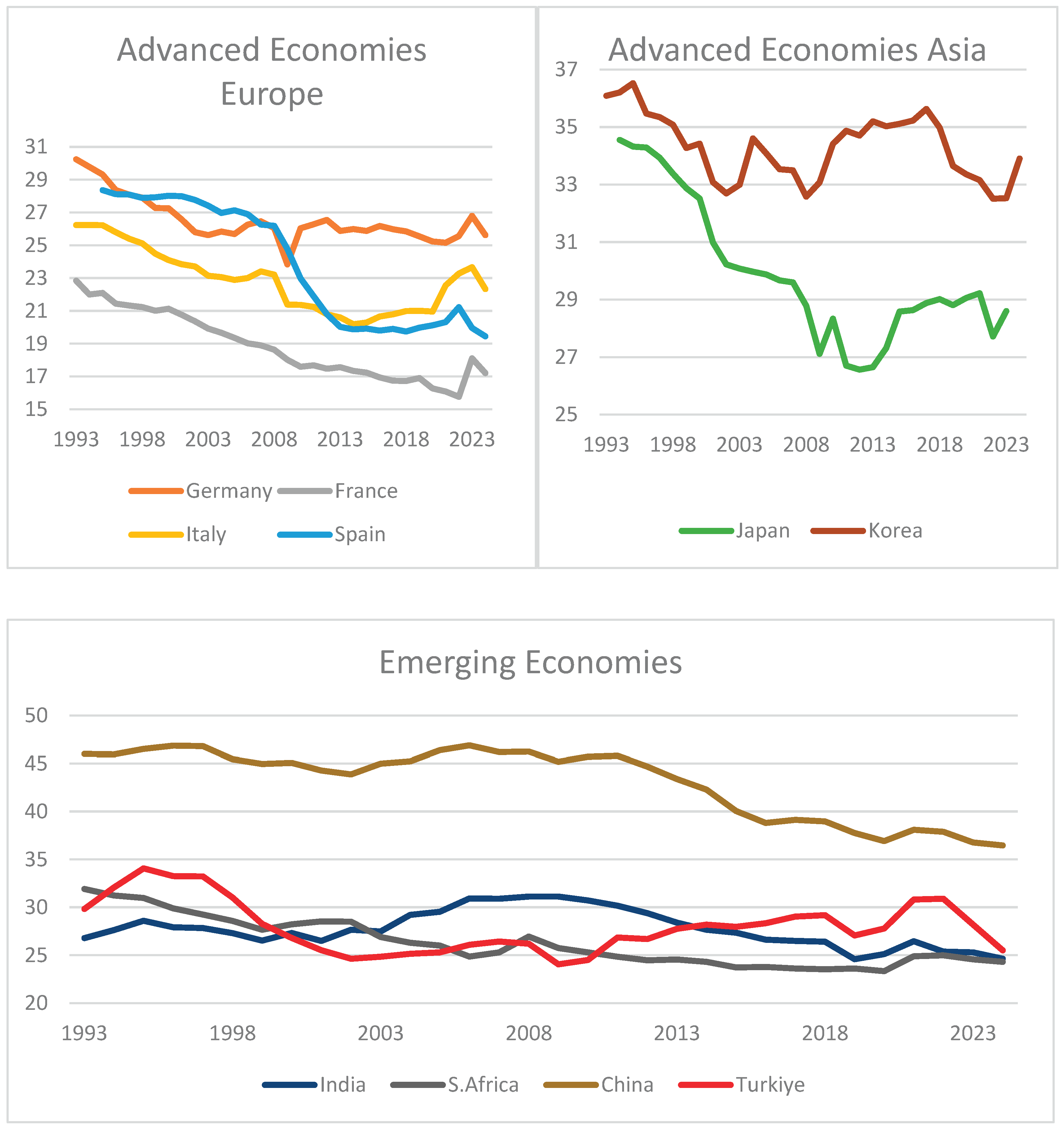

Table 1.
Descriptive statistics.
| Variable | Obs | Mean | Std. dev. | Min | Max |
| FDI | 319 | 1,686301 | 1,536117 | -0,89387 | 12,60853 |
| GFCF | 320 | 25,33247 | 6,919438 | 13,05137 | 44,51877 |
| Trade | 320 | 52,05261 | 16,49794 | 15,72334 | 105,5663 |
| CPI | 320 | 101,0486 | 61,18073 | 0,335941 | 834,5931 |
| IVA | 316 | 28,25465 | 6,962084 | 16,08773 | 47,5574 |
| LFP | 320 | 69,31195 | 9,447879 | 50,89431 | 95,36911 |
| OP | 320 | 53,56129 | 31,21481 | 12,28 | 109,45 |
Table 2.
Variables CD test.
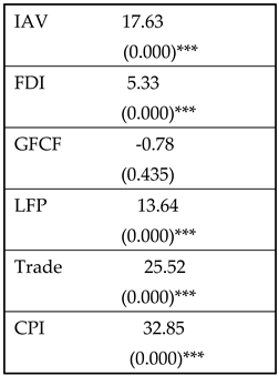
Note: *** p<0.01. The null hypothesis is cross-sectional independence.
Table 3.
Residual CD tests.
| The estimated alpha exponent = 0.55548 | |
|---|---|
| CD | CD* |
| -2.43** | 2.48** |
| (0.015) | (0.013) |
Note:** p<0.05. The null hypothesis is weak dependence.
Table 4.
Unit Root tests.
| Variables | IAV | FDI | OP | CPI | LFP | TRADE | GFCF |
| Level | -1.53 | -1.62 | -1.63 | -0.374 | -1.585 | -1.671 | -1.562 |
| First diff. | -4.2*** | -3.62*** | -4.939*** | -3.13** | -3.549*** | -4.024*** | -3.678*** |
Note: *** p<0.01. The null hypothesis is non-stationarity.
Table 5.
Cointegration Tests.
| Statistic | Value | Z-value | P-value | Robust P-value |
|---|---|---|---|---|
| Gt | -2.076 | -1.488 | 0.068* | 0.013** |
| Ga | -5.711 | 1.176 | 0.88 | 0.64 |
| Pt | -8.988 | -2.528 | 0.006*** | 0.04** |
| Pa | -4.925 | -2.062 | 0.024** | 0.02** |
Note: *** p<0.01, **p<0.05. The null hypothesis is no cointegration.
Table 6.
Slope Heterogeneity tests.
| Delta | Adj.Delta | ||||
|---|---|---|---|---|---|
| 4.444*** | 5.41*** | ||||
| p-value | 0.000 | 0.000 | |||
| HAC Kernel: bartlett | |||||
| with average bandwith 2.9 | |||||
| Variables partialled out: constant | |||||
| Cross Sectional Averaged Variables: IVA FDI GFCF LFP Trade CPI | |||||
Note: *** p<0.01. The null hypothesis is homogenous slope.
Table 7.
Presence of structural breaks test.
| Test Satistic Value | Bai & Perron Critical Values 1% |
5% |
10% |
|---|---|---|---|
| 6.09 | |||
| 8.42 | 6.84 | 6.09 | |
| Estimated break points: 2000, 2008, 2014 | |||
Table 8.
Short run estimation results.
| (1) | |
|---|---|
| VARIABLES | CS-ARDL |
| L.IVA | 0.340*** |
| (0.0980) | |
| FDI | 0.0552 |
| (0.0687) | |
| GFCF | 0.152*** |
| (0.0565) | |
| LFP | 0.260* |
| (0.143) | |
| Trade | 0.0901** |
| (0.0418) | |
| CPI | -0.104* |
| (0.0605) | |
| OP | -0.000811 |
| (0.00767) |
Note: Standard errors in parentheses: *** p<0.01, ** p<0.05, * p<0.1.
Table 9.
Long-run estimation results.
| Constant | 29.25*** |
|---|---|
| (10.73) | |
| lr_IVA | -0.660*** |
| (0.0980) | |
| lr_FDI | 0.0526 |
| (0.0842) | |
| lr_GFCF | 0.233** |
| (0.0996) | |
| lr_LFP | 0.550** |
| (0.251) | |
| lr_Trade | 0.190*** |
| (0.0737) | |
| lr_CPI | -0.206* |
| (0.122) | |
| lr_OP | 0.00170 |
| (0.0118) | |
Note: Standard errors in parentheses: *** p<0.01, ** p<0.05, * p<0.1.
Disclaimer/Publisher’s Note: The statements, opinions and data contained in all publications are solely those of the individual author(s) and contributor(s) and not of MDPI and/or the editor(s). MDPI and/or the editor(s) disclaim responsibility for any injury to people or property resulting from any ideas, methods, instructions or products referred to in the content. |
© 2026 by the author. Licensee MDPI, Basel, Switzerland. This article is an open access article distributed under the terms and conditions of the Creative Commons Attribution (CC BY) license.
Copyright: This open access article is published under a Creative Commons CC BY 4.0 license, which permit the free download, distribution, and reuse, provided that the author and preprint are cited in any reuse.


