

Submitted:
15 July 2026
Posted:
16 July 2026
You are already at the latest version
Abstract
In 1970, Dana Scott proposed his highly influential ''mathematical theory of computation'' to define the relationship between the text of a program and what the program computes (or denotes) --- the ''semantics'' of the program. Scott used a complete lattice based on the ''information ordering'', with the bottom element representing undefined --- a program failing to terminate normally, thus producing no information. The top element, however, was unused. Hence most subsequent applications of denotational semantics have used mathematical structures that avoid top elements. We suggest that the information ordering is relevant not only to semanticists, but also to working programmers, as a basis for determining if a program component or a computation is correct according to their intentions. We also suggest that a return to the use of complete lattices is called for if we wish to broaden formal semantics to allow it to encompass programmer intentions. That is because often those intentions permit more than one runtime behaviour for a given input. For example, several declarative debugging tools allow a programmer to declare that a runtime call is ''inadmissible'', loosely meaning the called program component should never be used with such input. If the input is garbage, the programmer does not care what garbage is output --- all results are acceptable, which can be modeled by the top element of a complete lattice. In this paper we explore the connections between the information ordering, correctness of computations and programs, and debugging. We present a general theory and describe several instances where the intention for what our logic/functional code computes plus what it actually computes can be described by elements in a complete lattice. This extends both the theoretical basis and practical flexibility of declarative debugging and reasoning about partial correctness and gives an attractive mathematical framework that encompasses our intentions, our programs and what they compute.
Keywords:
logic programming
; functional programming
; semantics
; partial correctness
; declarative debugging
; specification
; information ordering
; complete lattice
1. Introduction
Work on programming language semantics gives a mathematical view of the relationship between a program and its runtime behaviour — what a program computes, if anything (we will refer to this as the computation semantics). It is important and useful for several things. For example, it can be used to help track down bugs in programming language implementations such as compilers. A mathematical view is even more useful if it also encompasses what the programmer intends the program to compute (what we call the intended semantics). This can be used to help track down bugs in application code by providing a mathematical basis for debugging tools and gives a more holistic view of program development. See Figure 1 for a graphical depiction.
Some theoretical accounts of programming may lead us to believe that separate consideration of intended semantics is redundant because our job as programmers is to write code that computes exactly what we intend. However, (we claim) that is not how code is written. Our intentions often underspecify what is computed and can permit more than one behaviour. For example, if we code a merge sort algorithm, we will typically have a function or procedure called merge. The intention behind the procedure can reasonably be described informally as “merge two sorted lists to produce a sorted list containing the multiset of elements of the input lists”. This does not specify what should be computed when the inputs are not sorted lists and different codings that satisfy the description above compute different results for such input. Often there is no one-to-one relationship between what we intend and what is computed.
Of course it is impossible for us to ascertain what goes on in the mind of all programmers, and programmers do not all necessarily have the same intentions. However, we offer the following arguments in support of the claims made above. The first is introspection: the intention of the authors of this paper definitely underspecify behaviour in many cases. Second, the way programming is taught often uses underspecification: the description of merge above would not be out of place as a programming exercise for students. AI systems based on large language models such as ChatGPT and Gemini have learned to code from us and are generally good at producing code for a merge function but do a poor job at explaining what the code computes in general. Third, even formal methods for program development such as the Vienna Development Method allow underspecification. VDM-SL, a specification language for functions, supports preconditions that are assumed to hold (if they do not, any behaviour is permitted) and postconditions that are relations (rather than functions of the arguments) [? ]. Some programming languages also support preconditions. Fourth, practical experience with declarative debugging of logic/functional programs has led to support for imprecise intentions: the better debuggers allow the programmer to declare that a call is “inadmissible” (loosely meaning it should never have occurred) rather than deem the behaviour correct or incorrect. The saying “garbage in, garbage out” is an acknowledgement that we make assumptions about how our code is used and if used in other ways the result is garbage; for a given garbage input, we generally permit any garbage to be output. An alternative meaning for inadmissibility is that any behaviour is acceptable.
Given that our intentions are generally not identical to program behaviour, having a mathematical view of computation that explicitly includes our intentions is desirable. The applications range from educating programmers in how they can think about their code to formal specification languages and verification tools. In this paper we focus on applications to declarative debugging tools. Inadmissibility was introduced to declarative debugging for purely practical reasons, but with a mathematical theory there can be a better understanding and further practical advances. At the core of declarative debugging there are comparisons between program behaviour and what is intended. Sometimes intentions are described formally, such as those in formal specifications, preconditions in code and embedded test cases. More commonly, they are only in the mind of the programmer but declarative debuggers extract this information by asking questions. An appropriate mathematical view can help us design programming environments and guide programmers in corresponding ways of thinking about the correctness of their programs. Different mathematical views can be used depending on the programming language and what flexibility is supported, such as the use of inadmissibility. The approach we suggest here is aimed at supporting reasoning about partial correctness only — whether a program computes a correct result assuming it terminates normally.
The earliest work on a mathematical view of programming language semantics proposed using a complete lattice based on the information ordering [1]. The lattice contained all the possible data values manipulated by the code and all the possible mathematical functions corresponding to what the code can compute. The bottom element of the lattice stood for an absence of information (corresponding to computing nothing, due to an infinite loop or some other source of undefinedness, which is always a possibility in Turing-complete languages). The top element was present purely for mathematical convenience — no program or data object would be assigned this element as its meaning. Subsequent work on denotational semantics preferred other structures based on the information ordering where there is no top element, such as chain-complete partial orders.
In a previous paper [2] we showed how a complete lattice could be used as a mathematical foundation for declarative debugging in the logic programming context. The lattice in that case is one of truth values (Section 3.5 provides more detail). The ordering corresponds closely to the idea behind Kleene’s “strong” three-valued logic [? ]. The bottom element corresponds to nothing being computed, whereas the (additional, relative to Kleene’s logic) top element corresponds to inadmissible (that is, any behaviour is acceptable, according to our intentions). The other two elements, true and false, are incomparable in the information ordering. A program is (partially) correct if, for each ground atomic formula (atom), the truth value in the intended semantics is (according to the information ordering) greater than or equal to its truth value in the computed semantics. That is,
- an inadmissible atomic formula may be true (succeed), false (finitely fail) or undefined (loop) in the computation semantics;
- a true atom may succeed or loop;
- a false atom may finitely fail or loop; and
- an undefined atom must loop.
The information ordering is useful in a number of contexts [2]. It can serve to (a) relate an atom to its definition in the program, giving a sufficient condition for partial correctness, (b) relate successive states of a computation, (c) characterise the classes of bugs in definitions found by declarative debugging, (d) describe the constraints on program behaviour imposed by specifications and type and mode declarations, and (e) give a basis for the correct use of approximation, in the sense of abstract interpretation. In particular, if a program behaves incorrectly, the information ordering is violated in the computation because a predicate definition contradicts the ordering (and a declarative debugger can be used to pinpoint the buggy definition). Thus, this view provides a powerful mathematical tool that encompasses our programs, what we intend them to compute, and what they actually compute.
This unifying view of computation is not restricted to just logic programming and one view of intended interpretations. In this paper, we give other instances and hope the reader will be convinced it is widely applicable and a good way of viewing computation for the purposes of reasoning about partial correctness. Some readers may be familiar with the information ordering being used for (approximations to) what is computed, where “less precise” often means “less is known” and lower in the ordering. It should be noted that less precise intentions means more is permitted and higher in the ordering. Note that although the framework does encompass nontermination, the information ordering is not the right tool for reasoning about (definite) termination. For that, quite different mathematical tools are required, based on well-founded orderings, hence separating the concerns of partial correctness and termination is beneficial.
The rest of the paper is structured as follows. We first summarise its contributions. Then, in Section 3, we describe the essentials of declarative debugging and sketch its history. We also summarise the basics of order and fixed-point theory, to prepare for Section 4’s denotational definition of a simple functional programming language. In Section 5 we propose our general scheme for unifying computation and intended semantics. We show how the functional language of Section 4 and previous semantics for logic programming [2] are instances of the scheme, give technical results concerning correctness, relate these to declarative debugging and propose an improved classification of bugs. Section 6 shows that debugging of Horn clause programs conceived classically (that is, using two-valued logic) also complies with our framework. In Section 7 we return to functional programs, discuss the limitations of equational reasoning and how declarative debugging with inadmissibility fits with our scheme. We then, in Section 8, Section 9 and Section 10, discuss the case where a programmer can consider several but not all possible results correct, covering the case of functional programs with sets of values returned, and logic programs with sets of interpretations. In Section 11 we briefly discuss other language paradigms and Section 12 concludes.
2. Contributions
This paper essentially generalises our previous work [2] on logic programming semantics. It presents a general scheme for viewing the semantics (both computed and intended) of programs and gives multiple instances of the scheme to illustrate its usefulness. Specifically, the contributions are:
- In general, computed and intended semantics are distinct, even for correct programs, because intentions are sometimes imprecise.
- Computed and intended semantics of an expression can be described mathematically as (possibly distinct) elements of a complete lattice based on the information ordering. The bottom element ⊥ corresponds to nothing being computed and the top element ⊤ corresponds to everything being permitted according to our intentions.
- Partial correctness corresponds to the intended semantics being greater than or equal to the computation semantics (in the information ordering). For example, if the computed semantics is ⊥ or the intended semantics is ⊤.
- The computation semantics of a program component (function, predicate, etc.) is equal to the computation semantics of its definition. More specifically, the computation semantics is the least fixed-point of some operator associated with the component definitions. For example, function definitions can be seen as equations with respect to the computation semantics.
- The intended semantics of a program component should be equal to or greater than the intended semantics of its definition — this is a sufficient condition for partial correctness. For example, the intended semantics of function can be more permissive than that of its definition without compromising partial correctness.
- The two ways in which the intended semantics can violate the ordering above correspond to the two general classes of bugs previously identified in declarative debugging literature [3]. For example, if the intended semantics of function is less permissive than or incomparable to that of its definition, the definition is buggy.
- A computation can be seen as a sequence of computation states, each of which can be given computed and intended semantics. The computation semantics is the same for each state. The intended semantics for successive states should remain equal or decrease — this is a sufficient condition for partial correctness. If it increases or is incomparable the final result may be incorrect and declarative debugging can be used to find a corresponding buggy definition that causes the computation to go wrong at such a point.
- Different programming languages and domains can be used, allowing different degrees of flexibility in the intended semantics our programs. The mathematical view can guide the implementation of corresponding declarative debuggers. For example, Horn clause logic programs can be viewed with classical (two-valued) interpretations, multi-valued interpretations (supporting inadmissibility) or sets of interpretations and functional programs can be viewed in ways supporting inadmissibility or sets of permissible values.
This paper does not give rigorous definitions and proofs for all the different instances of the general scheme. An instance for logic programming was fully developed in [2]. This paper generalises the approach, develops all the technical details for an instance that uses a simple functional language (in Section 4) and gives a broad brush view of how the approach can be applied in other cases. Similarly, the way declarative debugging can be adapted to different instances is just described informally with examples. Our aim is convince the reader that the scheme is a good way of viewing programming and that the details for any particular instance can be fleshed out without too much trouble.
3. Background
There are several areas of background information that we now cover and provide provide context for. The first is declarative debugging; for a more detailed review we refer to the survey paper Caballero, Riesco and Silva [? ]. The next is the approach to logic programming semantics [2] which this paper generalises. Basic results related to partial orders and lattices follow. Included in this section is Proposition 1, a result that relates solutions to equations and inequations used later. Finally, the domain of Scott [1] is described.
3.1. Declarative Debugging: Logic Programming Origins
Declarative debugging goes back to Shapiro’s concept of “algorithmic debugging” [4]. Its simplest instance is debugging incorrect answers in Horn clause programs, that is, pure Prolog without negation. A computed answer can be associated with a proof tree, each node of which is an atomic formula (an “atom” for short) which succeeded in the computation, with the children being the atoms in the body of the clause instance used in the proof. The debugging algorithm uses an “oracle”, which embodies the intended semantics (an interpretation of the program which maps ground atoms to true or false). If a successful atom is not valid (that is, not all instances are true) in the intended semantics, the tree can be searched by checking validity of atoms within it using the oracle. Ultimately the debugger finds an atom that is not valid but whose children are all valid, which corresponds to an “incorrect clause instance” — the clause is false in the intended semantics (and hence buggy). Thus an error has been precisely located.
The oracle typically relies on asking the programmer questions (for example, is a certain atom valid). However, it can be partially automated to limit the user dialogue. For example, if a particular atom is declared valid, any instance of it can be inferred to be valid. Answers can also potentially be stored across multiple debugging sessions and derived from trusted code, assertions or specifications [5,6,7]. Exactly what kinds of questions are asked, what type of assertions etc are supported, and what inferences are made by the oracle depend on the programming language being debugged, the classes of bugs being diagnosed, the debugging algorithm, and what kind of intended semantics is supported. For example, in the simple case of Horn clause programs above, the oracle just determines the truth of universally quantified atoms. In other cases the oracle may have to provide valid instances of atoms, determine the truth of existentially quantified atoms and universally quantified equations and determine if a functional expression is well-defined (possibly with both universal and existential quantifiers) [8].
The early (1980s) declarative debuggers for logic programs were implemented as modified meta-interpreters, taking advantage of Prolog’s meta-programming features. Such features allowed relatively fast construction of (portable) declarative debuggers.
3.2. Declarative Debugging: Other Declarative Languages
By the early 1990s it was natural to ask how declarative debugging might be extended to other declarative language paradigms [? ,9]. The utility of declarative debugging for functional programming languages using call by name or call by need semantics was obvious: the opacity of where and when execution step take place made a declarative approach to debugging very attractive. It was clear that higher-order functions in functional programming would complicate matters considerably, compared to the logic programming case, especially for languages such as Haskell which encourages curried function definition and partial application. Nevertheless, it has mainly been in the Haskell community that the goal of declarative debugging has been pursued [? ,? ,? ,? ,? ,? ,? ,? ,? ].
Since Haskell lacks the reflective capabilities of Lisp or Prolog, implementations generally have taken one of two directions. One is to implement a modified compiler and a runtime environment which builds a debugging tree while executing a program [? ,? ], the other is to use program transformation: modify the program to be executed, so that the program, in addition to its result, returns its associated debugging tree [? ,? ,? ,? ,? ]. For a comparison of these approaches, we refer to Caballero, Riesco and Silva [? ].
Approaches to declarative debugging of functional logic programming languages fall much closer to the work on logic program debugging than to the functional case [? ,? ]. Here, however, we also have the possible complication of laziness, as important languages use lazy narrowing [? ] for reduction.
3.3. Generalising Declarative Debugging
Naish [10] suggests a general scheme for declarative debugging, in which the computation is viewed as some kind of tree and the oracle maps nodes to either correct or erroneous. An erroneous node with only correct children is called a buggy node and corresponds to a bug in the code. Different languages and bug symptoms (for example, wrong answers from logic/functional languages plus missing answers in logic programming languages) require different trees and different oracles. Similarly, different classes of bugs can be discovered. Prolog can have incorrect clause instances and “uncovered” atoms (that cause incorrect finite failure or missing solutions). Functional languages can have incorrect equation instances and, for lazy languages, “unreasonable demand” bugs that erroneously cause deeper evaluation than was intended [8].
The trees used for declarative debugging most commonly have nodes corresponding to the final result of the evaluation of a procedure or function. For wrong answers in Prolog, this in the final instantiation of an atom that succeeded and in functional languages it is a function call and result with the function arguments and result in their final evaluated form. Logic variables and unevaluated expressions lead to oracle queries that use quantifiers. The children of a node correspond to atoms or evaluable sub-expressions in the body of the predicate or function definition, respectively. Such trees correspond to a “big step” view of the execution where procedure/function evaluation is seen as a single step (which can be decomposed into smaller steps). In this paper we will not discuss the trees in detail but note that other trees can be used. At the opposite extreme we have the “small step” view, a completely linear structure that follows the sequence of reductions in the computation, as used in the debugger for the functional logic language Escher [? ] (a tree can be formed by adding an artificial node at the root with all other nodes as children). This is a more procedural view of the execution. There are also many possible intermediate views, such as each node corresponding to the reduction of a sub-expression to weak head normal form. The two key things for debugging are that an oracle can be used to determine if the node is erroneous and that a node can be linked to (an instance of) part of the program source code.
Naish’s general debugging scheme defines buggy nodes but not how to find them. Many strategies for searching the debugging tree have been proposed. The first work [4] suggested bottom-up and top-down strategies plus “divide and query”, which results in fewer oracle interactions. There are many other proposals that attempt to make oracle interactions fewer, simpler or more intuitive [? ,? ,? ,? ]. Some strategies will only find top-most buggy nodes, whose ancestors are all erroneous. Although the oracle may ask questions, some user-interactions may actually be related to the search strategy. For example, the debugger may accept a “don’t know” answer to an oracle question and continue its search elsewhere in the tree, but possibly return to the same question if a bug cannot be found without that question being answered definitively. Alternatively, the user may say some sub-term is incorrect, and the search can be directed to the part of the execution where the term was created. In this paper we do not deal with search strategies but refer to Section 6.3 of Caballero, Riesco and Silva [? ]. We simply note that with some suitable tree representation of a computation and a suitable oracle, declarative debuggers can be constructed.
3.4. The Concept of Inadmissibility
The idea of inadmissibility was introduced to declarative debugging by Pereira [11].1 In the simple Horn clause case, as well as the oracle saying an atom in the proof tree is valid or not valid, the atom can be declared inadmissible, meaning the call should never have occurred. For example, the call may be “ill-typed” or some precondition may be violated. For illustration, consider the Prolog merge procedure in Figure 2.2 The procedure takes two sorted lists and merges them to produce another sorted list, as part of a merge sort program.
There are many variations of this merge coding that produce identical results when called with sorted lists — we can readily identify eight “equivalent” variants: namely, when the two elements of the input lists are equal, either one could be added to the output list first; and also we can swap the first two arguments in either or both the recursive calls and/or all the clause heads. All these eight codings work identically for a correct coding of mergesort. However, they all behave differently when the inputs are not sorted lists. The typical programmer will not know or care about the behaviour of merge in such cases. For example, merge([2|3],[1],Xs) succeeds (with Xs=[1,2|3], a non-list), whereas merge([2|3],[2],Xs) fails. For the intended meaning to exactly match the behaviour3, the programmer would have to understand the precise behaviour of their code for all inputs — a daunting requirement since replacing one of the eight versions of merge by any other version constitutes a change in intended meaning.
A bug in the mergesort code can result in merge being called in unexpected ways. If the intended meaning of merge does not match the behaviour, a declarative debugger may conclude a bug exists in merge rather than mergesort. To show the usefulness of “inadmissible” as an answer, let us change the mergesort example slightly. If we replace the last occurrence of Xs3 by Xs1, resulting in the code shown in Figure 3, the execution of the goal mergesort([4,3,4,2,1],R) proceeds as intended until the call merge([4,3],[1,2,4],R), leading to the answer R=[1,2,4,4,3]. By classifying the atom merge([4,3],[1,2,4],R) as inadmissible rather than wrong, a declarative debugger can shift its focus away from merge, allowing it to properly pinpoint the source of the bug. The inclusion of “inadmissible” as an option makes intended interpretations simpler for programmers and simultaneously allows declarative debuggers to do a better job. We also see it is a more realistic view of programming.
Such reasoning was the motivation for generalising the two-valued declarative debugging scheme to a three-valued scheme [3]. In this scheme, nodes in the debugging tree are labelled “correct”, “erroneous”, or “inadmissible”. As before, an erroneous node with only correct children corresponds a bug, an e-bug. An erroneous node with one or more inadmissible children and all other children correct corresponds another class of bug, an i-bug. Naish [12] argued that Prolog code is typically constructed using a combination of forward reasoning (if the clause head satisfies preconditions, or admissibility as we would say here, the same applies in the body) and backward reasoning (if the clause body is true then so is the clause head, assuming any preconditions are satisfied). The two classes of bugs correspond to failures in these two forms of reasoning.
Figure 4 shows the buggy clause instance from the bad mergesort version in Figure 3. The head of the clause instance corresponds to some debugging tree node and the atoms in the clause body are the children; the classification of the nodes by the oracle is given as comments on the right. The debugging algorithms must be adjusted to take account of the new class of bugs. Also, the oracle must change in order to support inadmissibility. Naish [13] gave a corresponding formal semantics for pure Prolog, which was later revised and extended [2]. This provided a theoretical basis for the kind of declarative debugging session illustrated in Figure 5, where users are asked if an atom is valid (in their intended interpretation) but also get the opportunity to say the atom is inadmissible. Although inadmissibility has also been used in debuggers for functional languages [? ,8], there has been no previous formalisation of the corresponding intended semantics.
The introduction of inadmissibility some 40 years ago drove a wedge between computation semantics and intended semantics. Inadmissibility is an acknowledgement that intentions are imprecise, and thus must be distinct from what is computed.
3.5. Two- Three- and Four-Valued Semantics of Logic Programs
As a semantic foundation for declarative debugging (as well as for type/mode systems, program analysis and specification) in logic programming, Naish and Søndergaard [2] proposed the use of four-valued logic as a unifying semantic domain, able to accommodate inadmissibility.
In traditional approaches to logic program semantics [14], an interpretation maps ground atomic formulas to the set of truth values, and a model is an interpretation that makes each program clause true. To make the connection between falsity and finite failure, and allow negation in programs, multiple clauses for a single predicate are typically combined into a single “if and only if” clause [15]. The clause body can be a disjunction and the clause head has distinct variables as the arguments. In all these approaches, two-valued logic is employed, as might be expected.
However, subsequent work on the semantics of logic programs embraced the fact that the presence of non-termination, or undefinedness, is unavoidable in a Turing-complete language, and as a consequence it is more natural to base semantics on a three-valued logic [16,17]. In that approach, the basic semantic domain is , ordered as shown in Figure 6(a). The element represents undefinedness, and the order relation ⊑ on truth values is defined iff , thus expressing the information content of the values, with and being equally informative and holding more information than .
Naish and Søndergaard [2] took this three-valued approach one step further, by using the set of four truth values as basic semantic domain. Where again represents undefinedness, or lack of information, the element represents an information glut, leading to the ordering shown in Figure 6(b). The resulting structure is a bilattice [? ] with two interlaced orderings, namely the information ordering defined by iff , and a “truth ordering” defined by iff .
Naish and Søndergaard identified an important use of , the fourth truth value, as representing “inadmissible” queries in declarative debugging (whence the name ). With this, all meaningful decision-making interaction between programmer and debugging tool came down to comparisons using the information order ⊑.4 If the intended semantics of the heads of all predicate definitions are greater than or equal to that of their respective bodies5 the ordering also holds between successive execution states and between nodes and their collective children in the debugging scheme, there are no buggy nodes, and the computation is guaranteed to be correct.
3.6. Equations, Inequations and Fixed Points
We consider a declarative (logic, functional, or functional logic) program as a tuple of definitions (of predicates or functions). Definitions may be recursive or mutually recursive, and hence order and fixed-point theory is used to define their meaning. We now briefly recall the relevant concepts.
A binary relation on a given set X is a partial order iff R is reflexive, transitive and antisymmetric. If R is a partial order, we refer to as a poset. We shall use symbols such as ⊑ and ≤, with infix notation, for partial orders. Note that the identity relation , which we write as `=’, is a partial order. Hasse diagrams are traditionally used to depict posets graphically, and in accordance with that diagrammatic convention, we read as “x is below y (or they are equal).” We may also write as . A pair of elements x and y, for which neither nor holds, are incomparable.
Let be a poset. An element is minimal in Y iff . And y is the (unique) least element in Y iff . Maximality is the dual notion: is maximal in Y iff , and y is the greatest element in Y iff . Clearly any poset can be extended so that it has a least (and/or) greatest element (while remaining a poset). A least (greatest) element is often written as ⊥ (⊤).
Let be a poset and let . An element is a lower bound for Y iff for all . We say that x is a greatest lower bound for Y iff, for every lower bound for Y, . Dually x is an upper bound for Y iff for all , and again, x is a least upper bound for Y iff, for every upper bound for Y, . When a greatest lower (least upper) bound exists, it is unique, and we denote it (). We write (“x meet y”) for and (“x join y”) for .
A poset for which every subset possesses a least upper bound and a greatest lower bound is a complete lattice. Note that a complete lattice therefore has a least element and a greatest element .
Given a poset , we equip the function space with pointwise ordering. That is, overloading the symbol ⊑, iff . A function defined on a poset is monotone iff for all . An element is a fixed-point for iff .
The well-known Knaster-Tarski theorem [? ] establishes that
- 1.
- every monotone function on a complete lattice has a non-empty set of fixed-points,
- 2.
- Y itself is a complete lattice, and
- 3.
- The least fixed-point, .
Given monotone function on complete lattice L, we may, for reasons that will become clear, ask about the function defined by
Proposition 1.
Let be a complete lattice and let be monotone. The function defined by is monotone and .
Proof.
f and ⊔ are monotone, so is too. It follows that has fixed-points, and it is easy to see that is a fixed-point for . Namely, by definition of , . To see that is the least fixed-point for , consider an arbitrary fixed-point y for . We have , that is, y is an element of the set . So and, by item (3) of the Knaster-Tarski theorem, , hence . We conclude that . □
Proposition 1 is of interest to us because, as we shall argue, programmer intentions do not always reflect a strict reading of declarative programs as equations or "if and only if" statements. A program usually takes the form of a set of mutually recursive “equations”
where the are objects (functions or predicates, say) that are defined recursively through the use of monotone functionals . It is well understood that one can find least fixed-points of the by finding the least fixed-point of , defined by
We claim that programmer intentions behind the writing of (1) generally corresponds to the weaker set of constraints
which we could also write as
Proposition 1 then establishes that the reading (2) is not in conflict with a computation semantics provided in the form of a least fixed-point characterisation. We can freely think of the “equations” as having a direction, the direction expressing information order.
3.7. Denotational Semantics
We follow the Scott-Strachey approach to semantics. That is, we want to map program text to mathematical objects that somehow describe the “meaning” of programs and program components. In Section 4 we show this mapping concretely for a small functional language. Before that, however, we need to discuss what sort of mathematical objects are in use and how spaces of values can be defined, and well-defined at that.
As our language will allow us to write integer numerals, let us start with the set of integers, . As all “semantic” domains, it will be equipped with structure. We follow Scott’s original approach and introduce the flat lattice that has Hasse diagram
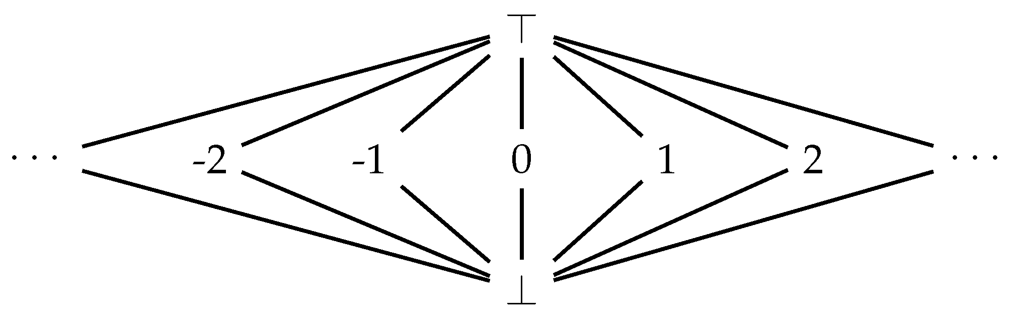
So in fact the domain is
ordered by iff . The ordering is intended to capture degrees of information. The element ⊥ represents the absence of information, ⊤ an over-supply, and the integers are all equally informative.
Two comments should be made up front: (1) If we were dealing just with integers as semantic objects, there would be no need for this marshalling; the reason why we order objects according to information content becomes clearer when we consider the meaning of functions and other infinite objects. (2) The element ⊤ will not appear as the meaning of any program component, according to the semantic functions defined in the next section. Scott [1] nevertheless chose to include ⊤, because of perceived convenience, preferring to have complete lattices for semantic domains.6 In our case, the inclusion of ⊤ is very deliberate, as it could conceivably be the “intended” meaning of some expression. We return to that claim in Section 5.
We also want to include data structures such as tuples and lists. Again we follow Scott [1] and use the versatility of three simple ways of building new lattice domains. Given domains and (and overloading ⊑), we use:7
- The Cartesian product with ordering defined by iff .
- The sum which is formed by taking the disjoint union of and , except the least element of is removed, as is the least element of , replacing the two by a new shared ⊥. While the lower points of and are thus coalesced, the upper points are left separate, and a new ⊤ is added, above all other elements. The order ⊑ is inherited from the input domains.
- The function space , with ordering defined by iff .
The ordering of functions gives a clear sense of how information content is captured: contains partial functions; for some says that f is undefined for that x. So means that f and g agree on all arguments for which they are both defined, but g may be defined in cases where f is not. If f, g, and h are different functions and then f and g can be seen as approximations to h, with g being a better, or closer, approximation than f. This realisation is critical because the only way to define an infinite object may be as the limit of a chain of increasingly better finite approximations.
Using sums and products (generalised), now define
to capture the finite lists with elements taken from D. Then we can define, using recursion, a domain suitable for giving meaning to the languages used later in the paper:
Cardinality considerations make it clear that we cannot thereby have defined a domain that includes all possible finite or infinite lists, nor can it contain all possible functions. In fact, the importance of Scott’s work [1] lay in determining suitable restrictions on semantic domains and functions that would ensure that domains would be well-defined by recursive definitions like the one above, and that only computable objects were included. With Scott domains only objects (including functions) that are finite or can be determined as limits of countably infinite chains of finite approximations are thus included. The key is a suitable notion of continuity and the reading of as the space of all continuous functions [1].
We have now introduced the necessary machinery for a more formal treatment of the concept of intended semantics in the setting of a functional programming language. Language features or variations beyond what we use in Section 4 are readily incorporated. For example, for a typed language it is natural to introduce separate domains for separate types. Additionally, for some applications it may be necessary to work with less abstract semantic definitions, in order to capture aspects of runtime behaviour considered relevant for those applications. For example, Launchbury [? ] gives both operational and denotational semantics for a lambda calculus with let-bindings, capturing weak head normal form reduction. Launchbury’s semantics elegantly models the runtime sharing of data structures and enables reasoning about a program’s space consumption.
The ideas presented in the current paper would also seem to carry over to functional logic programming in a straightforward way. For example, the community behind the lazy functional logic language Curry have developed denotational definitions for that language [? ], and Curry too is an example of a programming language that has been well supported by programming environments that include declarative debugging [? ].
4. A Denotational Semantics for a Simple Functional Language
We now give a denotational definition for a simple untyped functional language that captures what is computed but ignores details such as data structure sharing. The aim is to provide an example that we can then use to show how a concept of intended semantics can be incorporated. A program is a collection of function definitions:
To run a program, an additional expression must be given. For example, we could have this definition:
and the expression h(3). In more detail, we assume the following syntax:
Here X is the syntactic category of variables, C that of data constructors (we count constants as nullary constructors), A that of builtin operations, and F that of user-defined function names. We leave C under-specified but assume C contains at least integer numerals and constructors (of arity 2) and (of arity 0) for the construction of lists. A is also under-specified, but we assume A contains the usual integer operations, as well as selector functions and for lists, so that and .
We make the usual static-semantic assumptions: In a definition, each variable used on the right-hand side is one of the variables used on the left-hand side, the latter are all different, and function and operator arity is respected.
It is straightforward to define a small-step operational semantics. That semantics gives rise to a trace which may be finite or infinite. If it is finite and ends in then is the result of evaluating e on that program (or perhaps may be an expression that indicates abnormal termination). In the context of declarative debugging, it seems fair to restrict attention to finite traces.
We now give a denotational definition of the semantics using the domain (3) defined in Section 3.7. Without any loss of generality, we make the assumption the program has n function definitions, , that all have the same arity k, as this allows a simple approach to variable and function lookup.
Definition 1.
In Def. 1’s equations we overload symbols to let and give the meanings of constructors and builtin operations (on the left-hand side of the equation is the name (), on the right-hand side the corresponding function). The distinction between the categories C and A is based on how computation steps treat elements of the two. Builtin operations can be rewritten in computations, different functions and arguments may lead to the same result and thus the function and arguments may not be possible to extract from the result. Data constructors are not rewritten, different functions and arguments lead to different results and the arguments and function can always be extracted from the result. For example, the operation named “*” means the multiplication function and the meaning of “1*0” is the integer 0 (from which we cannot recover the function or its arguments). The data constructor named “cons” can mean an abstract list building function and the meaning of “cons(1,nil)” is the list containing just the integer 1, from which we can recover the function and its arguments. We can also view data constructors in a less abstract way, with the meaning essentially being the identity function, so the meaning of “cons(1,nil)” is simply cons(1,nil).
The operator selects the ith element from a tuple. The “whererec” clause defines as the least fixed-point of a functional of type (note that the components of tuples here are continuous mappings , all part of D). The subscript in indicates this is the computation semantics; later we introduce for the intended semantics.
Program examples later in the paper will freely use (standard) syntactic sugar for tuples and lists.
5. A Mathematical Theory of Correct Computation
This section defines our general view of programming language semantics and gives key technical results, the most important contributions of the paper. We show how the scheme can be applied to logic programming [2] and the functional language defined in Section 4; we hope the reader is convinced it can also be applied to many other languages quite easily. We assume programs and expressions have the forms described in Section 4, possibly with minor syntactic differences and well-formedness restrictions. For example, in logic programming, Definition 1 of [2] uses a pair rather than equation for each definition of a program component (predicate) and the expression on the right side of each definition is a disjunction of conjunctions of predicate symbol applications — other data constructors can only appear within these (there are also existential quantifiers but these could be made implicit and dropped from the syntax). Similarly, many languages have well-typedness restrictions.
For a program that defines n components (such as functions or predicates), our scheme requires the following:
| The domain and ordering, forming a complete lattice | |
| The computation semantics of a program | |
| The intended semantics of a program |
The semantic domain D, a complete lattice with a partial order ⊑, minimum ⊥, and maximum ⊤, contains the meanings of all symbols and possible expressions in the program. All semantic mappings are monotone and compositional. gives the computation semantics of each of the n components of p and is the least fixed-point of the definitions. gives the intended semantics of each of the n components of p and is not constrained by p but there may be constraints imposed in order to align it to various software tools such as debuggers. The semantic mappings for other symbols are fixed. Distinct expressions composed entirely of data constructors (including constants) are mapped to distinct values that are incomparable in the ordering. We can think of such a term as being mapped to (a possibly abstract version of) itself. Other “builtin” symbols have fixed mappings such as “+” being mapped to the addition function.
For our functional language of Section 4, the Scott domain is used. To align the semantics with declarative debuggers that support inadmissibility8, functions in should map completely defined terms (those not containing ⊥ or ⊤) to either completely defined terms or ⊤. For the logic programming semantics [2], the domain has the four truth values as described in Section 3.5. The ordering of these elements is the only thing crucial for the results that follow but to fit the general scheme and follow the tradition of denotational semantics we include additional elements in the domain corresponding to data structures and mappings.9
Our results concern the intended and computation semantics of expressions that contain no free variables and may appear as the top level expression to be evaluated or the right side of a component definition. All differences between intended and computation semantics of expressions stem from differences between intended and computation semantics of the program. However, to simplify notation we assume the program p and its semantics is fixed and implicit. We use the following notation:
| The computation semantics of an expression (given ) | |
| The intended semantics of an expression (given ) |
For the logic programming semantics [2], only the meaning of logical formulas is needed, which can be determined from the program semantics and the meaning of the logical connectives. For our functional language of Section 4, these meanings are defined using the generic semantic function for expressions applied to the computation or intended meaning of the program and some (unused) variable assignment :10
The information ordering for expressions aligns with partial correctness: the evaluation of expression e to result , is considered correct if . As usual, if , nothing is computed, which is acceptable for partial (though not total) correctness. Additionally, means every possible behaviour is acceptable. Generally, the range of will be elements relatively low in the lattice and can never include ⊤. Elements higher in the lattice can be in the range of and correspond to intentions that are more permissive (less precise). Inadmissibility is maximal permissiveness/imprecision and is the only form of imprecision used in semantics and declarative debugging to date.
To eliminate variables in expressions we use instances of component definitions, called head groundings in [2] (Definition 2):
Definition 2
(Instance of a program component definition). An instance of a definition , is an equation , where there are no variables in any expression and is r with each occurrence of variable replaced by .
The key sufficient condition for correctness relates the left and right sides of instances of definitions in the program. The computation semantics of the two sides are equal, as is the case in the classical view of correctness of intentions. However, a weaker sufficient condition for partial correctness is that the left side is greater than or equal to the right side in the information ordering, that is, the intended semantics is a solution to the corresponding inequations.
Definition 3
(Reducing program component definition). A definition , is reducing if for all instances .
Note that if a definition is not reducing there is an instance such that and if evaluates to exactly what is intended, , then the evaluation of is incorrect. The only way incorrectness can be avoided is for the evaluation of to result in something strictly less than what is intended, such as the evaluation not terminating.
There are two independent ways of reasoning about correctness. The first just uses lattice theory. We lift the lattice over D to a lattice over using component-wise ordering and overload ⊑ to apply to semantics of programs as well as expressions. Partial correctness for individual expressions can be lifted to partial correctness of programs as follows (essentially Theorem 1 of Naish and Søndergaard [2] in a more general setting).
Proposition 2.
Given a program p, if then every expression evaluation using p is partially correct. That is, for all expressions e, .
Proof.
for all components in p and this is the only source of difference between the computation and intended semantics of expressions. The result follows from the compositionality and monotonicity of the semantic functions. □
We now prove the main result from the lattice theory perspective, Corollary 1 of Naish and Søndergaard [2] in a more general setting:
Proposition 3.
Let p be a program. If all definitions in p are reducing then p is partially correct, that is, .
Proof.
is the least fixed-point, the least solution to the equations in the program component definitions. This is also the least solution to the corresponding ⊒ inequations — see Proposition 1 and the discussion after that result. Since all definitions are reducing, is also a solution to the inequations. □
We now give a more procedural view of correctness. The procedural definition of the programming language must align with the denotational definition of the computation semantics above. A computation is a sequence of expressions. Each computation step rewrites a sub-expression, replacing the left of a component definition instance by the right, or replacing a builtin symbol application by another expression. For completeness, we also model runtime errors, by allowing a special error application that may be the result of a rewrite11. Rewriting continues until there are no more sub-expressions to rewrite (thus the expression only contains data constructors), or the expression contains error. The result of the computation is the final expression. This is a familiar view of computation in functional programming. For logic programming each expression can be a disjunction of conjunctions and each step rewrites a conjunct [2] (Definition 10); nested disjunctions are avoided in this proposal, but could be modelled by a builtin operation. The final expression is a disjunction of conjunctions of equations (from which a set of computed answer substitutions could be extracted).
If all component definitions are reducing, successive states of a computation must satisfy the information ordering. If the intended semantics remains the same or moves lower in the lattice for each computation step, the final irreducible expression must be correct. We can prove correctness of computations that terminate normally by considering the procedural semantics, using minimal lattice theory:
Proposition 4.
If all program component definitions are reducing, any finite computation with no runtime errors is correct, that is, .
Proof.
The procedural semantics aligns with the denotational computation semantics, so . Since only contains data constructors, . All program component definitions being reducing implies , due to the compositionality of the semantic functions and monotonicity. The result follows from transitivity of ⊒. □
This procedural view is what allows declarative debugging. The steps of a computation should ideally satisfy the information order. An incorrect result can only be produced if at least one step violates the ordering and the corresponding program component definition instance must also violate the ordering. This is what is found by declarative debuggers (using a tree-based view of the computation rather than a linear one). There are two ways in which the ordering can be violated for a definition instance : or and are incomparable. These two cases align with the definitions of e-bugs and i-bugs [2,3]. For an e-bug, l is admissible (), all reduced applications in r behaved correctly and none were inadmissible (so ) but , so and are incomparable (inadmissibility is the only form of imprecise intention in this debugging scheme). For an i-bug, l is admissible and there is at least one reduced application in r that is inadmissible (has ⊤ as the intended semantics) and all others are correct; occurrences of ⊤ can propagate outwards, consistent with monotonicity, and result in . An e-bug moves the intended semantics “sideways” in the lattice whereas an i-bug moves it up the lattice (and it can subsequently move down along a different path), both potentially leading to incorrect results.
Declarative debugging can be seen as the search for an e-bug or i-bug, with the help of some representation of a computation and an oracle that gives the intended semantics. We propose the following (re)definitions:
Definition 4
(i-bug, e-bug). An i-bug is an instance of a program component definition such that . An e-bug is an instance of a program component definition such that and are incomparable.
These definitions have several advantages over the original definitions:
- They elegantly reflect the role of the information ordering in correct computation and exactly complement the definition of a reducing program component definition.
- They are entirely declarative, based on our intended meaning rather than a particular tree-based view of a computation.
- They are more general, allowing for more flexible imprecise intended semantics, not only inadmissibility.
- A node in a debugging tree containing expression l and result r can be classified as correct if , otherwise it is erroneous — a uniform view of correctness with no special case for inadmissibility needed.
- The propagation of ⊤ (or imprecision more generally) in r is left to the semantics. For example, a sub-expression of r that means ⊤ may not affect the overall result and if ⊤ is not propagated by the semantics, debugging can be more accurately directed to code that is the actual cause of incorrect behaviour (an example is given in Section 7.2).
Allowing imprecise intentions by using a complete lattice and viewing correct computation in terms of the information order has very wide application. To demonstrate this, the following sections give several instances of the theory we have described here.
6. Horn Clauses with Classical Logic
Logic programming was originally based on Horn clauses and classical logic. This has many limitations (such as no inadmissibility, no negation and no distinction between finite failure and infinite loops) but its simplicity and elegance are attractive. It can also be viewed as an instance of our theory of correct computation as follows.
The lattice contains classical (two-valued) interpretations and is based on the truth ordering rather than the information ordering with true being the top element (elements that don’t correspond to atomic formulas sit between true and false and can largely be ignored). is the least fixed-point of the “immediate consequence” operator (if the body of some clause instance is true in S, the head is true in )12. This is the set of atoms with successful derivations, the least model of the program and the intersection of all models. The notion of correctness is that no “wrong answers” are computed — everything true in is true in . The ordering of the lattice can only be violated by clause instances of the form in the intended interpretation and such clause instances are found by the simplest form of declarative debugging.
7. Functional Programs with Inadmissibility
This section demonstrates how the Scott domain described in Section 3.7 can be used for computation and intended semantics of functional programming languages, providing a theoretical basis for declarative debuggers that support inadmissibility. We use Haskell syntax for familiarity. First, we discuss some of the problems associated with the classical way of reasoning about correctness of functional programs.
7.1. The Limitations of Equational Reasoning
The practical motivations for using inadmissibility in declarative debugging of functional programs is the same as that for logic programs — Figure 2 can easily be translated into a functional language. Just as (classical) models of the logical theory do not accurately describe the intended semantics of the Prolog code, equational models (advocated for Escher by Lloyd [? ]) do not accurately describe the intended semantics of functional programming versions. Traditionally, equational reasoning has been advocated for reasoning about and transforming functional programs [? ] and is one reason cited for developing a denotational semantics for Curry [? ].
As we have already suggested, a literal reading of the equals sign in functions definitions can be dangerous. The “equations” are intended to have a direction. This manifests itself, for example, in the paradox that the unfolding of a function definition (the program transformation that takes an expression , instantiates f’s definition accordingly, and replaces by the definition’s instantiated right-hand side) generally is a harmless, whereas unconstrained folding is not.
We argue that inadmissibility (what will be ⊤ in our suggested domain) also causes significant problems for equational reasoning. Consider the Haskell definitions in Figure 7; the Haskell Prelude contains definitions of last and maximum. The intentions are that both list_last and list_last’ return the last element of a non-empty list and both ord_max and ord_max’ return the maximum element of a non-empty set, represented as a sorted (ordered) list. Using equational reasoning it appears that equations 3 and 4 are equally valid, both equating renamed versions of list_last and ord_max. However, because of the difference in admissibility (any non-empty list versus only sorted non-empty lists) ord_max’ is correct but list_last’ can result in wrong answers, as exemplified by the definition of one.
We argue that although “=” in the definition of these functions can be viewed as equality in the computation semantics, it should be viewed as ⊒ in the intended semantics. For Figure 7, the intended meanings of all equations except Equation 4 satisfy this ordering.
7.2. Semantics of Functional Programs with Inadmissibility
We use a Scott-style domain — see Section 3.7 and the examples assume support for lists. Unlike the logic programming case where we only care about the ordering over truth values, here we care about the ordering over an infinite number of values. Figure 8 shows some of the domain.
First order values are shown on the left. In the middle of the lattice we have all the fully defined values — numbers, pairs (products) of numbers and all the other data structures such as lists (not shown here). Below this we have partially defined values, with the completely undefined ⊥ at the bottom. For strict languages this part of the lattice collapses; there are no partially defined values. Above the completely defined values there is a mirror image of the lower part of the lattice with ⊤ replacing ⊥13. The computation semantics does not use ⊤, any term containing ⊤ or any function returning a term containing ⊤.
Functions are shown on the right — we use examples from Figure 7. The computation semantics is at or below the middle of the lattice for all functions. Total functions, such as merge14 appear in the middle; below them are partial functions that return ⊥ in some cases. Here we assume last and maximum yield ⊥ when applied to empty lists. The computation semantics of the other versions of last and maximum are the same as these, given by the equations in the program, and are not displayed separately. A variant of maximum that returned for empty lists would sit in the middle of the lattice, just above maximum.
Above the total functions there are functions that are inadmissible (return ⊤) for some calls; these may appear in the intended semantics. We assume that in the intended semantics list_last and ord_max are inadmissible for empty lists, so they are above (the computation semantics of) last and maximum, respectively. Additionally, the intended semantics of ord_max is above that of list_last because it returns ⊤ in strictly more cases (empty or unsorted lists) and for non-empty sorted lists it returns the same result as the other functions. This graphically illustrates the reason for the bug in Figure 7.
Consider the evaluation of one, given the definitions in Figure 7. The successive computation states are one, list_last’ [2,1], ord_max [2,1], maximum [2,1], …2, with respective intended meanings 1, 1, ⊤, 2, …2 (the computation semantics is 2 throughout). Where the intended semantics goes from 1 to ⊤, the information ordering is violated, due to the equation that violates the ordering, and this is what ultimately causes the wrong answer (going from ⊤ down to 2 is not a problem). Declarative debugging can be used to find where the problem arose in the computation and pinpoint the code that caused it.
The tree used in debugging to represent the computation has a function call and the result in each node. For the big step view, these are in their most evaluated form and each node has a child for each function call evaluated in the right side of the equation used. For the wrong answer returned by one we can use a tree with a node for one that has a single child for list_last’ [2,1] that has a single (inadmissible) child for ord_max [2,1] (where all these nodes have 2 as the value returned). The oracle can ask if a function call is intended to equal the result, with inadmissibility being an option (indicating the intended result is ⊤) on a par with true and false. Figure 9(a) shows a possible corresponding declarative debugging session, which finds an i-bug. This is (arguably) the most straightforward approach.
With this approach, the programmer only needs to know the meaning of functions applied to fully evaluated expressions and the meaning will be either ⊤ or a fully evaluated expression, which should equal the result of evaluation. Comparison with the result of evaluation is only relevant if the meaning is not ⊤. The logic programming equivalent is more straightforward in a sense: just an assignment of a truth value (, or ) to an atomic formula.
Unevaluated expressions in function arguments and the result (for non-strict languages) can be replaced by universally and existentially quantified variables, respectively. For example, if f (Just <thunk>) evaluates to Just <thunk> (where <thunk> is unevaluated), the oracle can ask if . f (Just x) equals Just y [8], with inadmissibility being the answer if all instances of f (Just x) are inadmissible.
For higher order code and curried function definitions there are several practical challenges, such as displaying higher order values and building a good tree representation of the computation [? ]. The tree for one given earlier is not the only possible tree we could use to represent the computation. A mathematical theory that encompasses intended semantics allows us to better understand the design space for declarative debuggers and provide guidance in tricky cases. We now give three examples of this. The first is an alternative debugging tree for the example above. The one node could have two children: one for list_last’ (with no arguments) returning ord_max and another for ord_max [2,1] returning 2. With this second tree, the oracle must compare the two functions list_last’ and ord_max and it is important that the comparison uses ⊒, not equality. The wording of questions to the user (if such a tree is used) should reflect this (in Figure 9(b) we use => instead of =, for example). Debugging using this tree is more concise but also more abstract, relying on the user to understand the ordering over functions, not just inadmissibility. With this tree the only buggy node is list_last’. It would be classified as an e-bug according to the original definition [3], since list_last’ produces an incorrect answer and has no children. With the revised definitions it would be considered an i-bug, consistent with the classification made in the earlier tree and the ordering violation in the computation.
With trees that do not reflect the big-step semantics, oracle interactions can become more complex again. For example, suppose we have a function mylength that incorrectly returns 1 instead of 0 for empty lists, so mylength [one] incorrectly returns 2. Depending on the design of the debugger and strictness of the language, the user could be asked to compare the intended meaning of mylength [ord_max [2,1]] with another expression. If all functions in the intended semantics are “co-strict” (), the meaning of this expression is ⊤. However, that need not be the case: the intended meaning of mylength applied to a single element list could always be 1, even if the language is strict. This could allow a debugger to ignore the behaviour of ones and focus on finding the bug in mylength. It may be that insisting on co-strictness is a good overall compromise or perhaps it is best to avoid the issue entirely by only using big-step trees, but whatever the case, it is good to have a theory to inform the choice. Furthermore, it is important that the debugger documentation makes clear what constraints are imposed on intended semantics or how the programmer may think about their program in order to use the debugger effectively.
The final “tricky” issue we discuss is the treatment of runtime errors. One simple solution is to use ⊥ to model both nontermination and runtime errors. This loses potentially useful information. It is also possible to use values just above ⊥ in the lattice but below all other values. In our scheme neither of these options allows us to use declarative debugging for runtime errors because such results are considered (partially) correct — they are lower in the information ordering than what is intended. Some declarative debuggers, such as the one for the logical/functional language NUE-Prolog [? ], model runtime errors such as pattern match failure by returning a special error value and asking if expressions equal this value in the intended semantics [8]. Reductions that are expected to result in errors, such as head [] => error … are considered correct. This can be modelled by having error values in the middle of the lattice. However, another attractive option is for errors to be high in the lattice, for example, immediately below ⊤ but above other elements. The reduction of any expression to an error must then be either inadmissible or incorrect. The debugger could simply ask if such expressions are admissible. Note that if errors are higher in the lattice, Figure 8 would have last and maximum higher, but still below the intended semantics of list_last and ord_max, respectively.
8. Beyond Inadmissibility
Compared to the more classical approaches, inadmissibility allows us more flexibility in how we think about our code. However, there are occasions in programming when our code is called with expected inputs but there are still multiple possible behaviours that we consider correct. In functional programming there may be multiple correct results and in logic programming there may be multiple correct sets of answers computed. However, not all behaviours are considered acceptable. For example, we may have multiple different representations for the same abstract value and we don’t care (and possibly don’t know) which representation is computed but we want some representation of the desired value to be computed. As with inadmissibility, the intended behaviour is under-specified but inadmissibility only allows us to model cases where there is either a single acceptable behaviour or all behaviours are acceptable. Consider the representation of sets of integers by duplicate-free lists that are not (necessarily) sorted. The set has two possible representations: [1,2] and [2,1]. A computation that is intended to produce a representation of this set has two results that are considered acceptable and a programmer typically will not care (and sometimes will not know) which one the program will actually return.
The main examples we use here are based on multiple representations of the same abstract value but there are other similar uses of under-specification. Some algorithms call for under-specified operations where the acceptable results are not considered equal in any sense. For example, we may have an operation that returns an arbitrary member of a set, coded so the result is determined by the representation of the set.
9. Functional Programs with Sets of Values
We now propose domains that support both the more flexible view of intended semantics above and embed the computation semantics for a functional language. One suitable domain has already been suggested, for the computation semantics of the logic/functional language Curry [? ]. This could be used for the intended semantics of Curry without its nondeterministic operator “?” that supports the logic programming features. We will refer to this language subset as FC (Functional Curry) to avoid confusion. For our purposes, FC has no major difference from other lazy functional languages. This domain is rather more complicated than necessary. We give a brief summary below then propose a simpler, more abstract domain.
The semantics in [? ] does not deal with the full Curry language directly. Recent Curry implementations generally use a simplified intermediate language, FlatCurry, and the semantics is actually developed for the TFLC language, that reflects all the important semantic features of FlatCurry. Likewise, we don’t spell out any details linking a practical source language to the domain. Unlike the Scott domain, which is untyped and uses a complete lattice, the Curry domain is typed and for each type there is a CPO defined, using the information order. To handle expressions having multiple possible values, Hoare powerdomains are used: downward closed sets of terms of the corresponding CPO (often it is convenient to just consider the maximal elements of the sets; the downwards closure can be implicit). This results in a complete lattice appropriate for our intended semantics. The subset ordering is used for the powerdomain. Although function arguments denote sets of terms, the semantics uses monotone mappings from single values in the CPO to sets of values in the powerdomain. The language has explicit let bindings and the computation semantics uses the least solution to sets of equations (equivalent to the least fixed-point). The only way sets with more than one element can arise in the computation semantics is if the program contains the nondeterministic operator, thus in FC, the computation semantics has only singleton sets15 and failure. Returning failure is represented by the empty set of terms, the bottom element of the powerdomain lattice (failure as an input is represented by a bottom element in the CPOs).
A simpler, more abstract domain can be constructed by just taking the Hoare powerdomain of the Scott domain, with the semantics of expressions being downward closed sets of values from a single base domain. The powerdomain has a sub-domain that is isomorphic to the Scott domain, where elements of the Scott domain are mapped to sets with a single maximal element and ⊇ is used in place of ⊒. For example, (0,0) in the Scott domain is mapped to {(0,0), (0,⊥),(⊥,0),⊥}. These sets are used for the computation semantics. In the following examples we leave the downward closure implicit and write {(0,0)} for the set above. The top element of the Scott domain is not needed in either the computation or intended semantics. The (intended) meaning of a function for which some calls are inadmissible is the (downward closed) set of all functions in the Scott domain that have the correct result for admissible calls. The meaning of an application is the set of all where and are in the meanings of f and a, respectively. An inadmissible call can result in any value because some function in the set will return that value. Thus the meaning of an inadmissible call is the universal set, the top element of the powerdomain.
As in other applications of our theory, if all program components are reducing, the program is correct. Note that the definition of reducing depends on the definition of ⊒ for the domain, which is ⊇ in this case.
Consider the code in Figure 10, which represents sets as (not necessarily sorted) lists without duplicates. Intuitive intended semantics for such code using the domain above can be defined as follows. First, function calls with arguments that are not valid set representations are considered inadmissible and are dealt with as described above. Also, disjoint_union is inadmissible if the argument sets are not disjoint. The intended meaning of admissible applications of these functions is independent of the representations used in the arguments. For example, if then m[1,2] = m [2,1].16 When sets are returned from a function or are the value of a let-bound constant such as set12a, the intended semantics includes all valid representations of the desired result. Thus both set12a and set12b have the meaning {[1,2], [2,1]}. The meaning of disjoint_union includes all functions that return some representation of the desired result.
With this intended semantics the definitions are reducing: the ⊒ ordering (⊇ here) applies to the intended meanings of the left and right sides of every equation instance. For set12a and set12b the meanings of both sides are equal. For disjoint_union the meaning of the left side is typically a strict superset. For example, the meaning of disjoint_union [1] [2] is {[1,2], [2,1]} whereas the meaning of [1] ++ [2] is {[1,2]}. Also, if the right side of any definition instance is inadmissible, the left side is as well. The meaning of is2 is {2} and though the right side of the definition contains set12a, which can return one of two different representations, both these representations are mapped by max to the same value.
The declarative debugging algorithm can be essentially the same as the case with just inadmissibility. Care should be taken to make user interactions consistent with the view that expressions can have multiple acceptable values. For example, asking questions about the equality of expressions and what they evaluate to could be misleading. The main difference is how the debugging environment supports changes in code that do not affect the intended semantics. For example, the oracle may know that reducing set12a to [1,2] is acceptable but the code could be changed so set12a reduces to [2,1] — the oracle should not conclude this is incorrect. Given that singleton sets of acceptable answers are generally the norm, it would be good to allow the user to declare this. For example, if asked whether some reduction is acceptable, the user could respond that the expression is inadmissible, the answer is incorrect or the answer is correct and (perhaps optionally) whether there is only one correct answer in this case and/or all cases for this function.
10. Logic Programs with Sets of Interpretations
This section describes a domain for logic programming analogous to the domains for functional programming given in the previous section.
10.1. Motivation
As with functional programming, allowing multiple possible behaviours of code but not all possible behaviours is often useful, for example, the representation of sets used in Figure 10. Figure 11 has the Prolog equivalent and also has some extra code that illustrates additional potential problems that can occur with such Prolog code, which we discuss later.
One somewhat thorny problem for logic programming that can also be helped with this approach is higher order programming. Although Prolog has higher order features and thus higher order programming is possible, it lacks any theoretical foundation. Unification is central to logic programming and higher order unification is undecidable, making an elegant account of higher order programming difficult. Higher order programming in Prolog uses first order values to represent what we would naturally think of as higher order values and, if used with care, allows the kinds of higher order coding done in functional programming languages. As with the set example, there can be multiple representations of the same abstract value.
Figure 12 gives a simple example of higher order Prolog code using the call predicate with three arguments. Many Prolog system have this as a built-in but it can be coded simply in Prolog as shown. It is analogous to apply in functional languages: apply fn arg = res can be translated to call(Fn, Arg, Res). The first argument, Fn, is a representation of a function (or more generally predicate) that maps (or relates) Arg to Res, thus call(mergesort,[2,1],Xs) will bind Xs to [1,2]. This can be used to code other higher order predicates. For example compose can be coded as shown and used to compose two functions/predicates: compose(append([3]), merge([2]), [1], Xs) merges the lists [2] and [1] and appends the result onto [3], binding Xs to [3,1,2]. It can also be used in other input-output modes, produce multiple outputs and have multiple answers; compose(append(Xs), append(Ys), [2], [1,2]) has two answers.
Potential problems arise because of this flexibility with input-output modes when there are multiple representations of the same value. In Figure 11 both set12a and set12b return representations of the same abstract value. Predicate is2 calls set12a, resulting in one representation being returned and max computes the correct result from this. However, in bug2, both set12a and set12b are called and although they return the same abstract value, the two different representations do not unify so bug2 fails. Similarly, in Figure 12, bug123 fails due to to different representation of the identity function (or equality relation) failing to unify. Functional programming languages avoid this problem to a large extent because the main way two values can be compared for equality is by a call to an equality function. Some functional programming languages support generic equality and comparing functions results in a runtime error (though comparing two representations of a set may result in the wrong answer). Other languages have mechanisms such as type classes that allow different equality functions to be coded for different types (but not function types). Forms of pattern matching and case expressions can also compare variables to fixed first order values, which can be a source of bugs.
10.2. Technical Details
We start with the three-valued base domain of Fitting and Kunen shown in Figure 6(a) (there are additional elements for data structures etc that we will never need to compare; we ignore these in the description here). We don’t require inadmissibility as that can be expressed when we lift the domain, which is done in two steps. The first step is as before, a domain of interpretations, mappings from the Herbrand base to the base domain. The bottom element is the interpretation that maps every ground atomic formula to undefined. There is no top element but many maximal elements that map everything to true or false. The second lifting step creates a complete lattice by using the Hoare power domain of the (three-valued) interpretations. Domain elements are downward-closed non-empty sets of interpretations and the subset ordering is used. The bottom element is the singleton set containing the interpretation that maps everything to undefined. The top element is the set of all interpretations, which is similar to the top element in the four-valued approach where everything is mapped to inadmissible. Because it contains all interpretations, every ground atomic formula will be true in some interpretations and false in others.
The lattice of four-valued interpretations is effectively embedded in this domain. A four-valued interpretation is a partitioning of the Herbrand base into four sets, I, T, F and U (the atoms mapped to , , and , respectively). This corresponds to the set of all three-valued interpretations where members of U are , members of F are or , members of T are or and members of I are , , or . The subset ordering over such sets of interpretations preserves the information ordering over four-valued interpretations. There are also other sets of interpretations in this domain, thus it is strictly more expressive than the domain of four-valued interpretations.
In [2] the intended semantics is a single four-valued interpretation and “reducing” means the truth value of the left of a definition instance is that of the right, where is the ordering on truth values. Here, the intended semantics is a set of three-valued interpretations and reducing means the set of truth values of the left of a definition instance is ⊇ that of the right.
The domain we proposed is very complicated to work with in its full generality. We make several suggestions for intended semantics that reduce the flexibility somewhat but make it more manageable. First, avoid explicit use of undefined in interpretations. The actual domain elements will be the downward closure of the set, adding undefined as a possible answer wherever true or false appear. Explicit use adds minimal benefit (it is only useful if the intention is that something must loop) and classical logic is familiar for programmers whereas non-classical logics tend to meet resistance despite their elegance. Second, use a set of interpretations for each individual predicate, with the set of interpretations for the whole program being the cross products of the individual sets. That is, the possible intentions for each predicate are independent of the other predicates. This limits interaction between how we view different predicates. Third, use multiple interpretations only for inadmissibility and non-canonical representations of abstract values such as sets17.
Inadmissibility can be supported in user interactions in the same way it is done with current debuggers. Mathematically, it corresponds to a set of interpretations as follows. Each inadmissible atom is mapped to true in some interpretations and false in others. The set of interpretations has all possible combinations of these mappings for each inadmissible atom. The mappings for admissible atoms are independent of the mappings for inadmissible atoms. For example, with the inadmissible atoms max([],2) and max([],1) of Figure 11, all four of the possible mappings to true and false are present in the set of interpretations but for all the interpretations, max([1,2],2) is true and max([1,2],1) is false.
For non-canonical representations, we use the idea of input-output modes. Although this seems at odds with a declarative view, it is intuitive for programmers and when using non-canonical representations of values, programmers must be careful with the modes in which their predicates are used. Some predicates have non-canonical values in “input” arguments and interpretations for such predicates should not discriminate between the different representations of values — all should be included in each interpretation. For example, max([1,2],2) and max([2,1],2) should be true in all interpretations. For predicates that have non-canonical values in some “output” argument position, there should be a separate interpretation for each possible representation. For example, set12a([1,2]) should be true in some interpretations and set12a([2,1]) should be true in all other interpretations but no interpretation has both true or both false (that would correspond to set12a(Xs) being allowed to return two answers or no answers, respectively).
The first five predicate definitions in Figure 11 are analogous to the function definitions in Figure 10. Other than disjoint_union, the sets of truth values for the head and body of each head clause instance are the same. For disjoint_union there are instances such as disjoint_union([1], [2], [1,2]) which is true in some interpretations and false in some interpretations but the body, append([1], [2], [1,2]), is true in all interpretations, still satisfying the ⊇ ordering. However, for bug2 the ordering is violated: bug2(2) is true in all interpretations whereas the body is true in some interpretations but false in others. Specifically, there is an interpretation (the least model of the program) where the only true instance of set12a(Xs) is set12a([1,2]) and set12b([1,2]) is false. This results in finite failure of bug2(N). Similarly, bug123(A) of Figure 12 fails because there are interpretations for which the body is false.
Existing declarative debuggers for Prolog assume a single intended interpretation. The better missing answer debuggers [? ] could potentially conclude the bug is in bug2, but only if users give counter-intuitive answers to the questions the debugger poses.
Figure 13(a) gives an example, where y means yes and n means no. If the user says set12a([1,2]) is false or set12b([1,2]) is true or set12a(Xs) has true instances other than set12a([1,2]), the debugger (incorrectly) concludes there is a bug in one of these predicates. Although set12a and set12b have the same intended meaning, the oracle must treat them differently to correctly diagnose the bug. With sets of interpretations the bug can be correctly diagnosed without such counter-intuitive answers. The oracle implementation must be refined to distinguish different interpretations. Figure 13(b) gives an example, where in answer to the first question y means yes in all interpretations. In answer to the next two questions s means true in some interpretations and false in others. The last question is interpreted as asking if there is an interpretation where set12a([1,2]) is true and there are other true instances in that interpretation. This user interaction allows the debugger to conclude there is an intended interpretation in which the clause body is false but the head is true, violating the ordering (ideally, this should be explained to the user along with the bug location). Note that although there is (at most) a single answer to each call in this example, multiple answers can be supported in the same way.
11. Other Instances
We have not described in detail how inadmissibility and more flexible imprecise intentions can be incorporated into functional logic languages but believe it can be done relatively easily. The computation semantics for Curry is well developed [? ]. The most straightforward way to adapt this semantics would be to replace the CPO used for each type by a lattice, with ⊤ meaning inadmissible for that type. This isn’t strictly an instance of our scheme (which has a single domain for everything), but has the same “vibe” and can lead to the same benefits such as improved declarative debuggers.
Similarly, some language paradigms don’t fit with our view of computation based on steps that rewrite a single sub-expressions but we believe that having a single domain that incorporates what is computed and (imprecise) intentions is desirable. Program components in imperative and object oriented languages can use the values of local variables and potentially other values (global or inherited) and update multiple data structures as well as (sometimes) returning a value. Declarative debugging can be applied to such languages [? ,? ] but one of the challenges is to present all this information to users in a form that allows correctness to be determined (even for declarative languages there are major challenges when large data structures are used). For any programming paradigm, there are typically assumptions about how program components are used, inadmissibility and other forms of under-specification are important and having a suitable theory is useful.
12. Conclusion
Programmers have always had imprecise intentions for the behaviour of their code, hence what code computes is generally distinct from what is intended, even for correct programs. Previous work showed the importance of the information order for reasoning about partial correctness of logic programs where intentions can be imprecise by allowing “inadmissibility” (meaning any behaviour is acceptable), a concept with a long history. The information order relates the left and right sides of predicate definitions, successive states of a computation and nodes and their children in trees that represent computations in declarative debugging. It also gives insight into classes of bugs.
Here we have generalised these results to a much wider class of programming languages and imprecise intentions, and further improved the classification of bugs. A detailed treatment of the semantics of a simple functional language shows that the results from logic programming hold in this case. We also provide less formal descriptions of multiple other instances of our general theory, for both logic and functional languages and different forms of precision for programmer intentions. This very general approach gives a mathematical theory that relates our code, what it computes and what we intend it to compute. The theory can help us design better, more flexible declarative debuggers.
Theoretical computer science has usually been rather distant from the concerns of practical programming. The development of declarative languages has brought the two closer, but the theory of programming language semantics has been applied in a rather naive way when it comes to how programmers should ensure correctness of their code. By distinguishing computation and intended semantics but relating them in a single mathematical theory, we hope to remedy this.
Author Contributions
Conceptualization: LN, BP, HS; methodology: LN; formal analysis: LN, BP, HS; writing—original draft preparation: LN; writing—review and editing: LN, BP, HS; visualization: LN, HS. All authors have read and agreed to the published version of the manuscript.
Funding
This research received no external funding.
Conflicts of Interest
The authors declare no conflicts of interest.
References
- Scott, D.S. Outline of a mathematical theory of computation. In Proceedings of the Proceedings of the 4th Annual Princeton Conference on Information Sciences and Systems, Princeton, NJ, USA, 1970; pp. 169–176. [Google Scholar]
- Naish, L.; Søndergaard, H. Truth versus Information in Logic Programming. Theory Pract. Log. Program. 2014, arXiv:1305.014114, 803–840. [Google Scholar] [CrossRef]
- Naish, L. A Three-Valued Declarative Debugging Scheme. Aust. Comput. Sci. Commun. 2000, 22, 166–173. [Google Scholar]
- Shapiro, E.Y. Algorithmic Program Debugging; MIT Press: Cambridge MA, 1983; p. 232. [Google Scholar]
- Edman, A.; Tärnlund, S.Å. Mechanization of an Oracle in a Debugging System. In Proceedings of the Proceedings of Eighth IJCAI, Karlsruhe, Germany, August, 1983; pp. 553–555. [Google Scholar]
- Drabent, W.; Nadjm-Tehrani, S.; Maluszynski, J. The Use of Assertions in Algorithmic Debugging. In Proceedings of the Proceedings of the 1988 International Conference on Fifth Generation Computer Systems, Tokyo, Japan, 1988; pp. 573–581. [Google Scholar]
- Naish, L.; Dart, P.W.; Zobel, J. The NU-Prolog Debugging Environment. In Proceedings of the Proceedings of the Sixth International Conference on Logic Programming; Lisboa, Portugal, Porto, A., Ed.; 1989. [Google Scholar]
- Naish, L.; Barbour, T. A Declarative Debugger for a Logical-Functional Language. In Proceedings of the Eighth International Conference on Industrial and Engineering Applications of Artificial Intelligence and Expert Systems — Invited and Additional Papers; Melbourne, Forsyth, G., Ali, M., Eds.; 1995; Vol. 2, pp. 91–99. [Google Scholar]
- Naish, L. Declarative Debugging of Lazy Functional Programs. Aust. Comput. Sci. Commun. 1993, 15, 287–294. [Google Scholar]
- Naish, L. A Declarative Debugging Scheme. J. Funct. Log. Program. 1997. [Google Scholar]
- Pereira, L.M. Rational Debugging in Logic Programming. In Proceedings of the Proceedings of the Third International Conference on Logic Programming; Shapiro, E., Ed.; Lecture Notes in Computer Science ; 1986; Vol. 225, pp. 203–210. [Google Scholar]
- Naish, L. Verification of Logic Programs and Imperative Programs. In Constructing Logic Programs; Jacquet, J.M., Ed.; Wiley: Chichester, England, 1993; pp. 143–164. [Google Scholar]
- Naish, L. A Three-Valued Semantics for Logic Programmers. Theory Pract. Log. Program. 2006, 6, 509–538, [cs.LO/0508004]. [Google Scholar]
- van Emden, M.; Kowalski, R. The Semantics of Logic as a Programming Language. J. ACM 1976, 23, 733–742. [Google Scholar] [CrossRef]
- Clark, K.L. Negation as Failure. In Logic and Data Bases; Gallaire, H., Minker, J., Eds.; Plenum Press, 1978; pp. 293–322. [Google Scholar]
- Fitting, M. A Kripke-Kleene Semantics for Logic Programs. J. Log. Program. 1985, 2, 295–312. [Google Scholar] [CrossRef]
- Kunen, K. Negation in Logic Programming. J. Log. Program. 1987, 4, 289–308. [Google Scholar] [CrossRef]
| 1 | To set his method apart from Shapiro’s, Pereira referred to it as “rational debugging”. |
| 2 | A note on Prolog notation: [X|Xs] denotes a non-empty list with head X and tail Xs. |
| 3 | Or if the intended meaning is any (rather than the least) classical model of the program. |
| 4 | Other uses of the fourth value include Fitting’s logic-based programming language for distributed programming [? ] and as a way to understand mode systems [2]. |
| 5 | Programs are normalised so that each predicate definition uses a single “if and only if” clause where the body is a disjunction of conjunctions and connectives are defined using truth tables over the four values. |
| 6 | Subsequent development of denotational semantics tended to focus on chain-complete partial orders, or CPOs, e.g., [? ]. |
| 7 | Other choices are possible for product and sum, with choices implicitly determining whether data constructors force evaluation of their arguments or not [? ]. |
| 8 | See Section 7. |
| 9 | The restriction to computable mappings does have a minor impact. In rare cases, it can be useful for inadmissibility to be uncomputable [2]. The approach outlined here does not allow that. |
| 10 | Note that the intended semantics thus is required to agree with the computation semantics on all expression forms, including constructors, builtin operations, and the conditional (function calls of course are interpreted in accordance with ). |
| 11 | We discuss the semantics of runtime errors later. |
| 12 | There is actually an assumption of a fair search strategy here; Prolog normally uses a simple unfair search strategy using backtracking. |
| 13 | There are also values containing ⊤ and ⊥, not shown here. |
| 14 | For simplicity, we assume all the functions here are restricted to take (fully defined) lists of integers. |
| 15 | More precisely, downward closed sets with a single maximal element. |
| 16 | For simplicity, we assume is {[1,2]}, etc, rather than something more abstract. |
| 17 | The method we suggest can also be used for similar cases such as returning an arbitrary member of a set. |
Figure 1.
The three components we want to view mathematically.
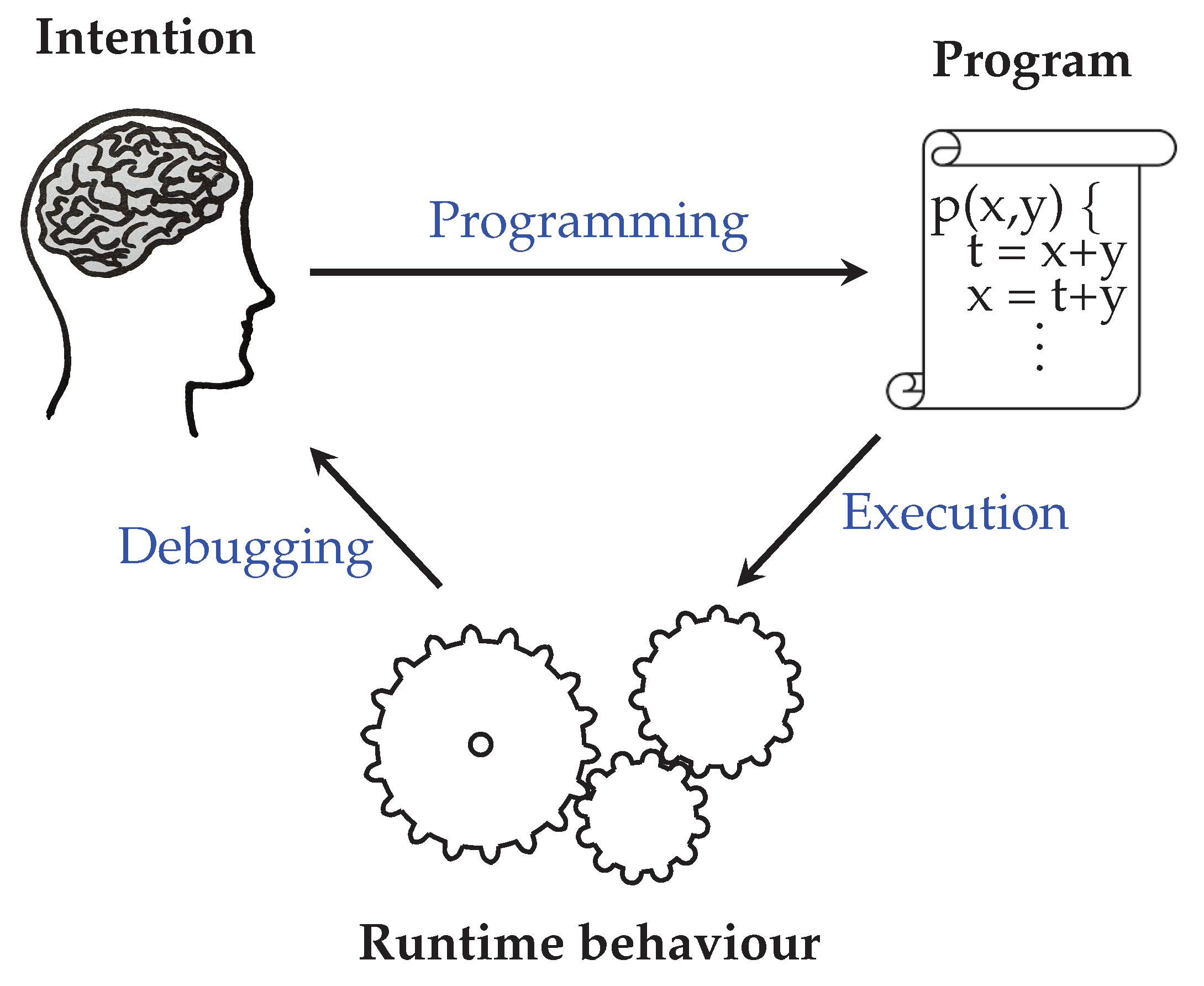
Figure 2.
Merge sort program.
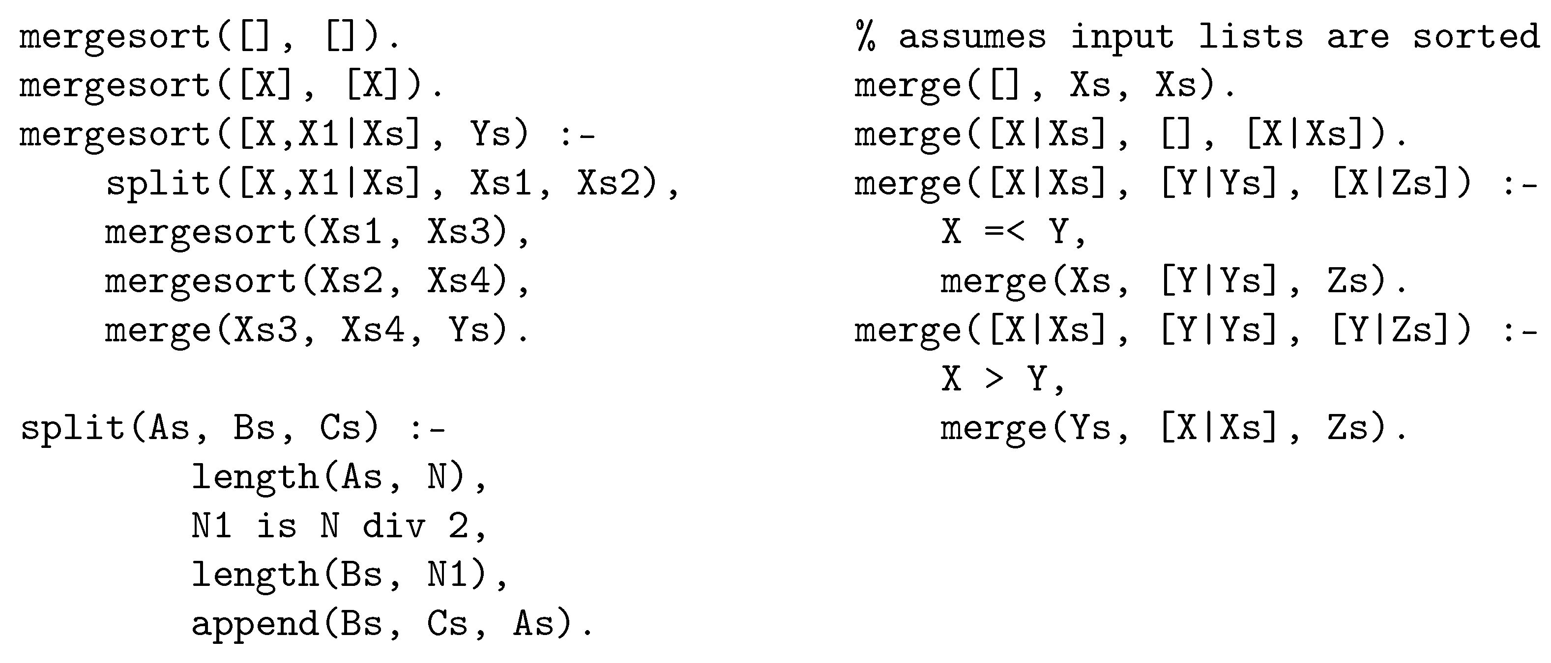
Figure 3.
Buggy merge sort procedure.
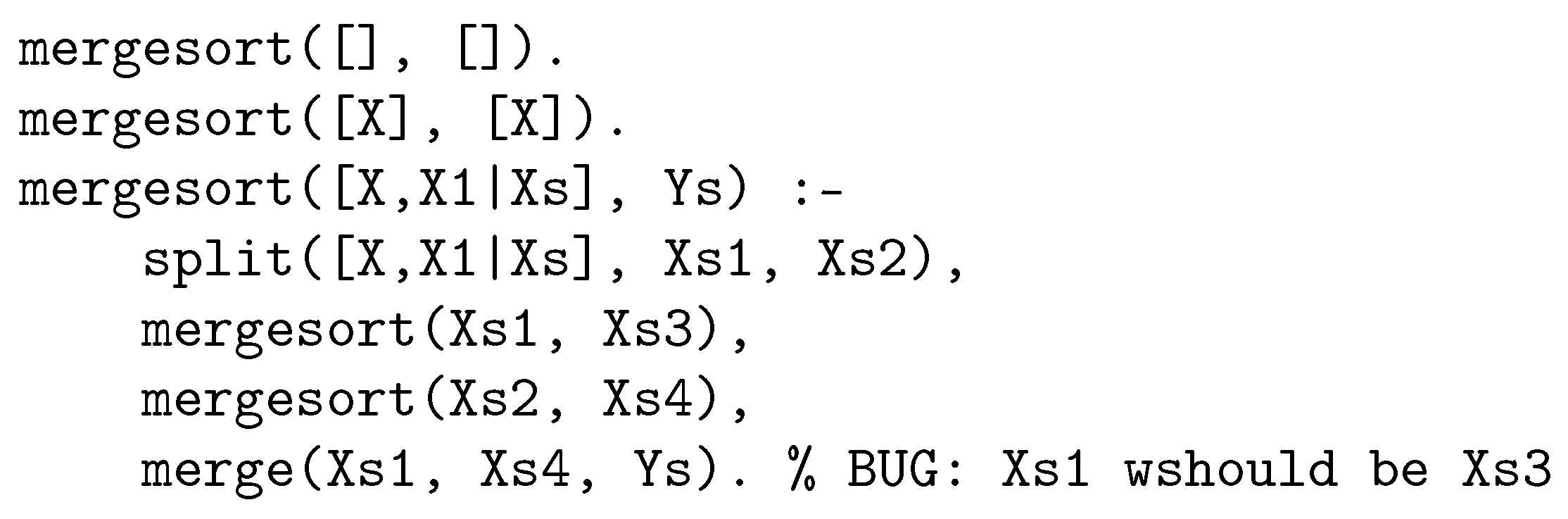
Figure 4.
A buggy clause instance due to inadmissibility.
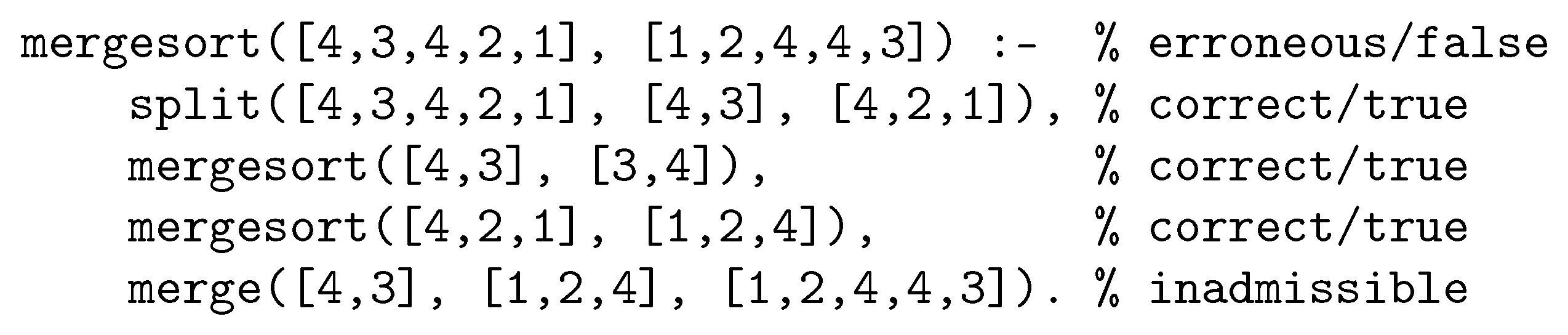
Figure 5.
Logic programming declarative debugging with inadmissibility.
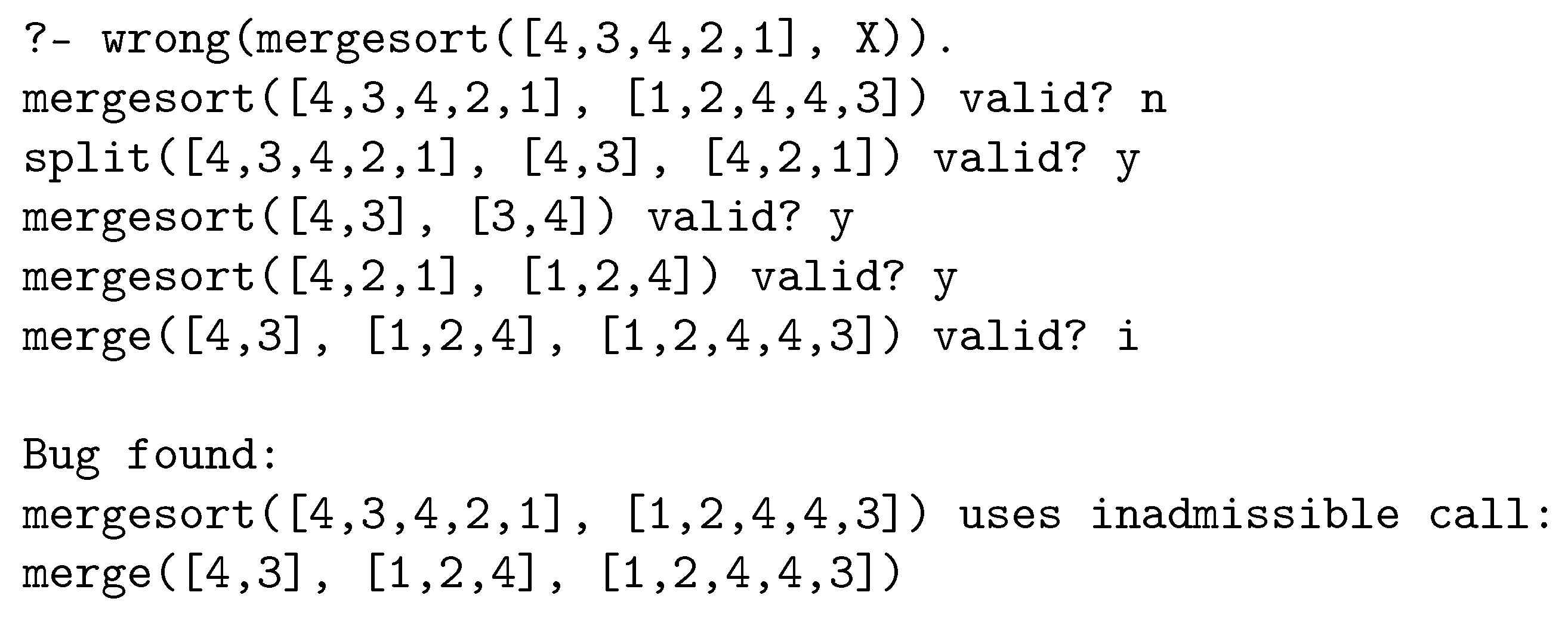
Figure 6.
Partially ordered sets of “truth” values.
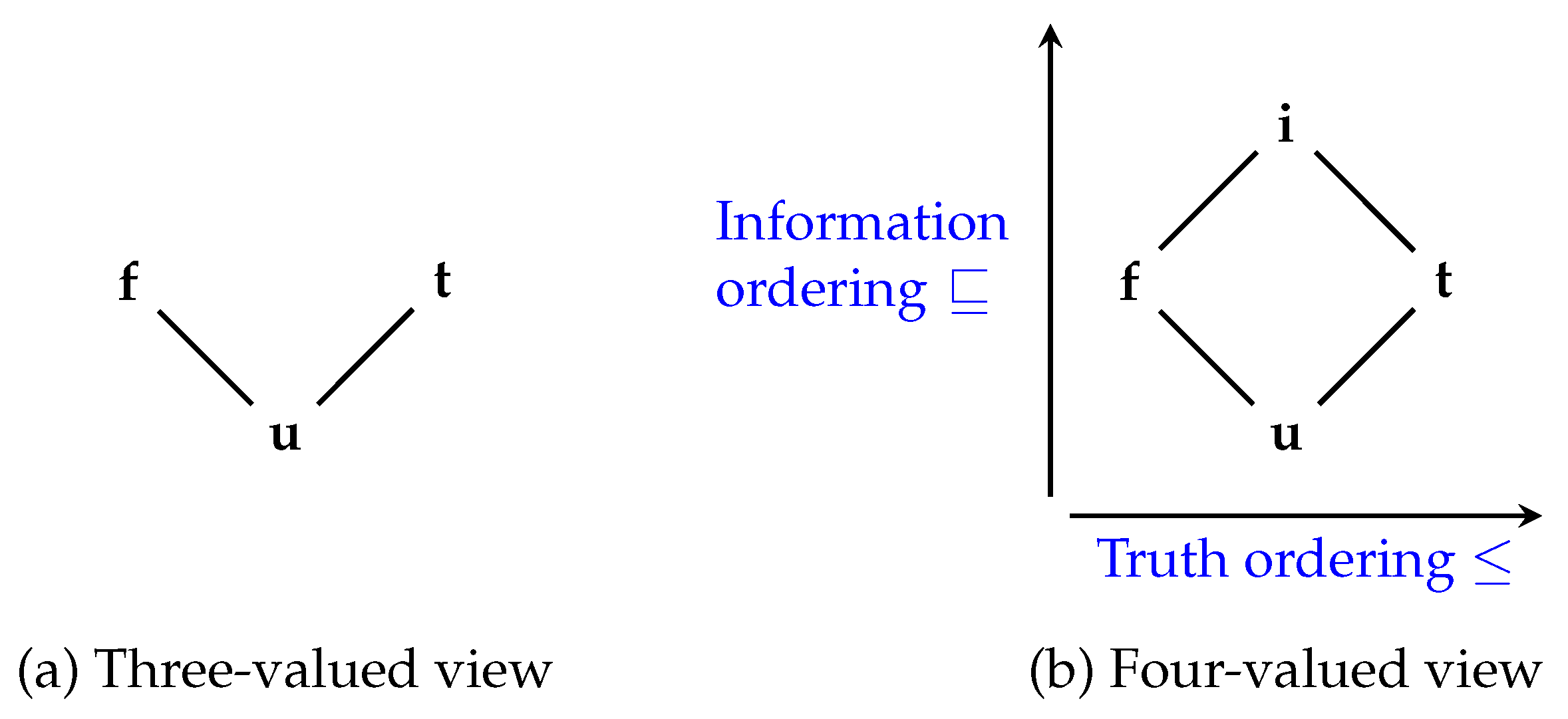
Figure 7.
Haskell code to return the last element of a list; sets represented as sorted lists.
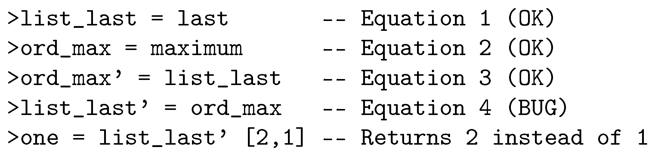
Figure 8.
Some of the domain for functional programs with admissibility.
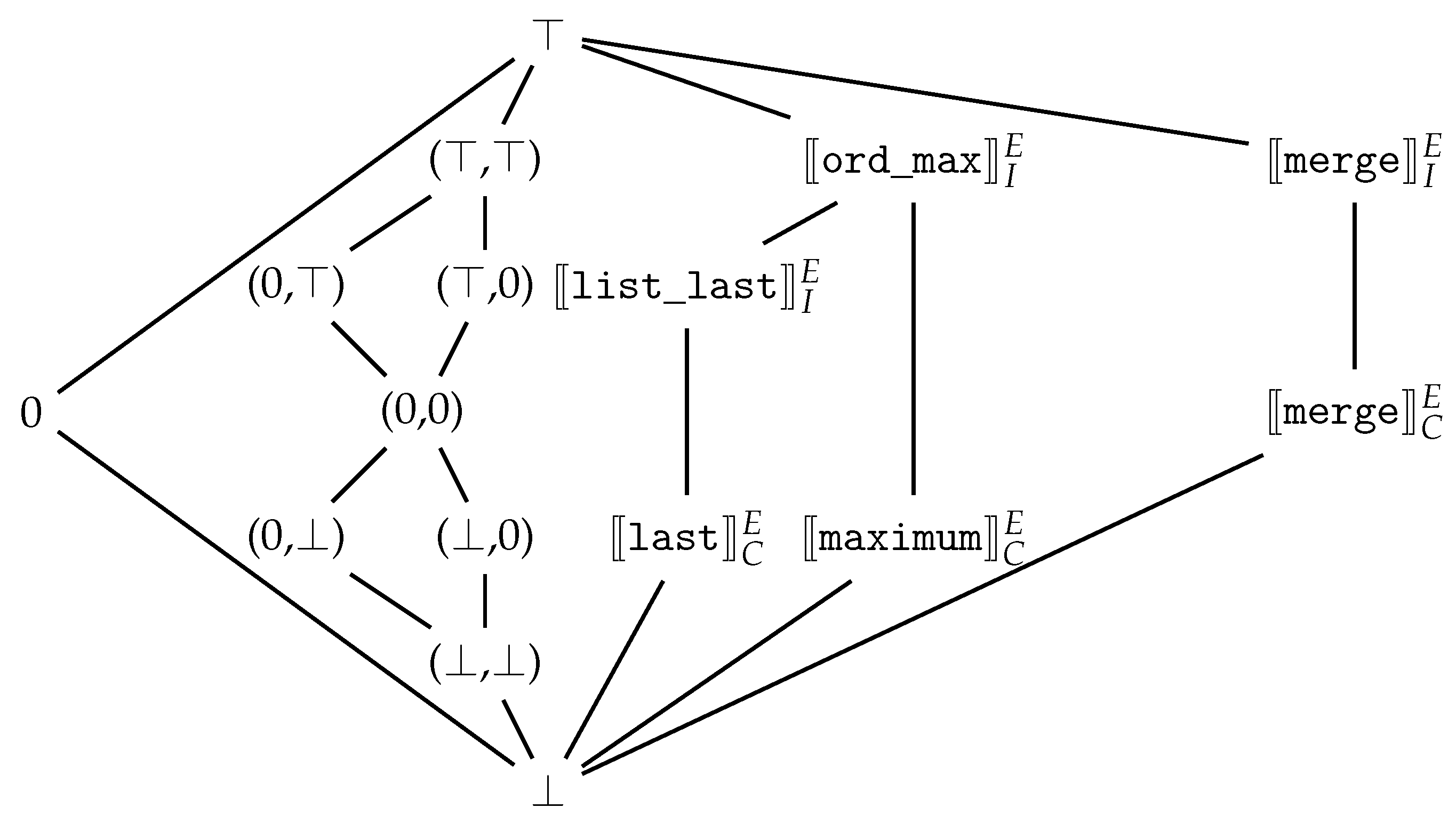
Figure 9.
Haskell declarative debugging with (a) inadmissibility and (b) currying.
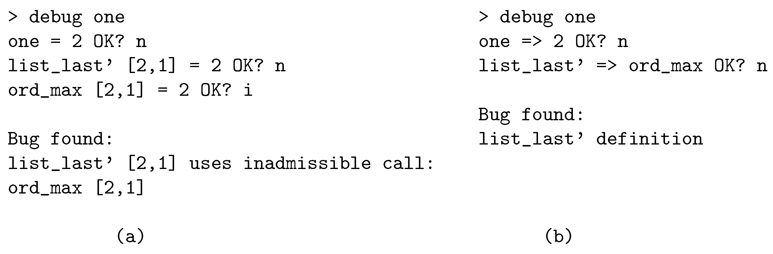
Figure 10.
Sets represented by (unsorted) lists without duplicates in Haskell.
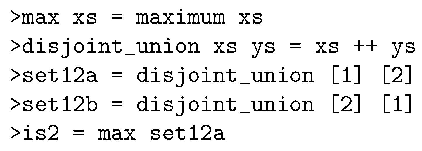
Figure 11.
Sets represented by (unsorted) lists without duplicates in Prolog.
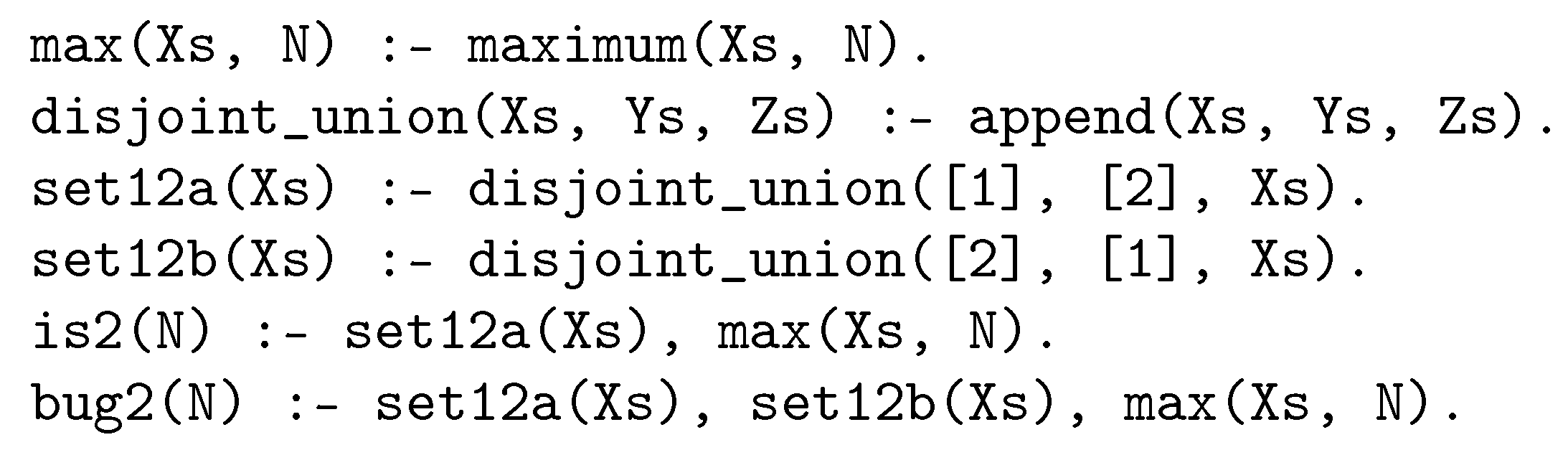
Figure 12.
Higher order programming in Prolog.
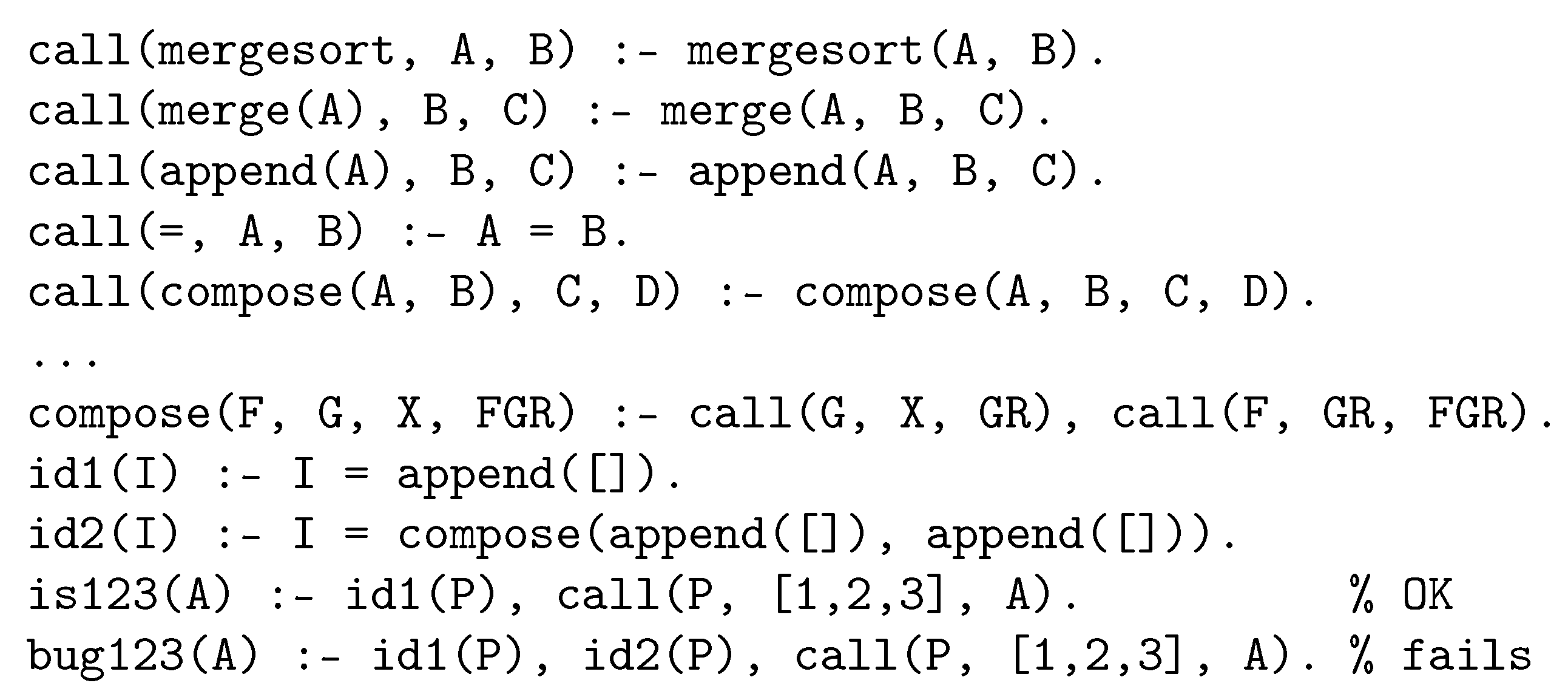
Figure 13.
Prolog declarative debugging with (a) single and (b) multiple interpretations.
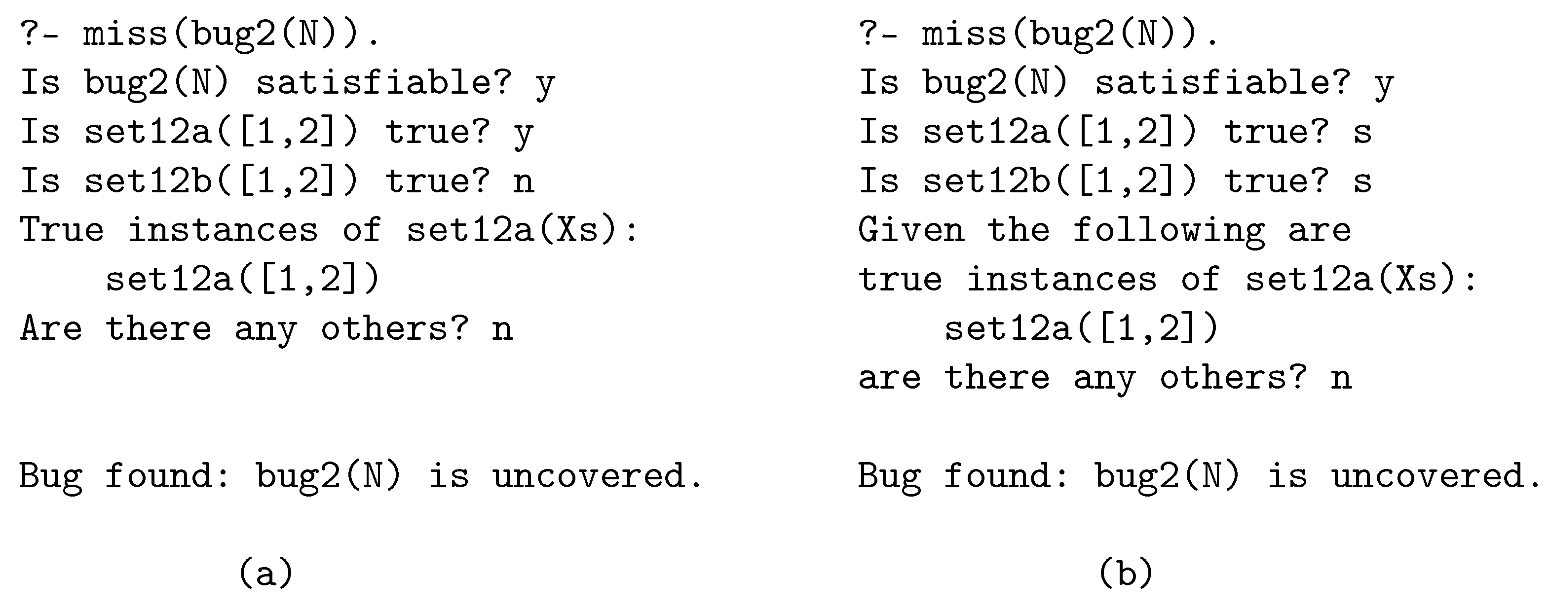
Disclaimer/Publisher’s Note: The statements, opinions and data contained in all publications are solely those of the individual author(s) and contributor(s) and not of MDPI and/or the editor(s). MDPI and/or the editor(s) disclaim responsibility for any injury to people or property resulting from any ideas, methods, instructions or products referred to in the content. |
© 2026 by the authors. Licensee MDPI, Basel, Switzerland. This article is an open access article distributed under the terms and conditions of the Creative Commons Attribution (CC BY) license (http://creativecommons.org/licenses/by/4.0/).
Copyright: This open access article is published under a Creative Commons CC BY 4.0 license, which permit the free download, distribution, and reuse, provided that the author and preprint are cited in any reuse.