

Submitted:
13 July 2026
Posted:
13 July 2026
You are already at the latest version
Abstract
This paper develops a new multi-stage method for image distillation which involves two well-known methods. At its first stage, our method creates a matrix from all training images. On the next stage, it adapts a modified principal component analysis (M-PCA) approach to transform the training matrix. On the third stage, the Singular Value Decomposition (SVD) further refines the matrix of the training images through low-rank reconstruction and controlled matrix row selection. On the fourth stage, rotation of small 2 × 2 matrix blocks on the entire left singular matrix is conducted. The upper m (user-selected number) rows of the reconstructed matrix are selected and transformed back to images, which we call distilled images. This dataset is significantly smaller yet retains the critical information needed for an accurate classification. We validated the novelties and the advantages of the new method applying the Baseline and ResNet50V2 CNNs and the public image databases Digit-MNIST, Fashion-MNIST, CIFAR-10, CIFAR-100, and BloodMNIST. Experimental results show that models trained on images distilled by our new method achieve efficient classification and outperform contemporary competitors, while substantially reducing training time compared to training on the original dataset.
Keywords:
image distillation
; principal component analysis
; singular value decomposition
; rotation
; image classification
; machine learning
1. Introduction
Deep neural networks (NNs) are difficult to train efficiently in the face of the exponential growth of data in modern machine learning (ML). Large-scale image databases have a huge demand for computational resources, including training time that may take days and memory requirements that exceed the standard hardware capacity [1,2]. To create a small but highly informative set of training samples that contains most of the important information of the original large dataset so that any model trained on those distilled images can achieve comparable results to training with the full dataset [3], the data distillation method is one of the most prominent solutions. Such a solution basically creates a small number of training samples, which saves computational time and memory and also makes the machine learning more efficient in resource-limited environments.
Note that gradient-based methods rely on NNs to extract information such as gradients and network parameters from the entire original dataset, which are then transferred back to another NN to produce the distilled images [4]. As a result, the distillation process itself is computationally expensive and time-consuming.
In contrast, the proposed new method is based on a modification of the PCA (M-PCA) and the SVD. Hence, we will denote it as M-PCA-SVD for Grey-scale images and QM-PCA-QSVD (Quaternion Modified PCA and Quaternion SVD) for colored images. Note that this distillation method is non-gradient and operates entirely through closed-form algebraic operations, requiring no NN training during distillation. This makes it significantly faster than gradient-based approaches, while still producing a compact and informative distilled dataset.
The present work directly extends the PCA-based framework designed to distill vectors from a set of vectors [5]. The new method works class-wise and first adapts the M-PCA to handle images by presenting the set of training images of a class as a single matrix. Further, this matrix is decomposed by the SVD. Then the left singular matrix is block-wise rotated, and the modified matrix is reconstructed. At the end, the upper m (user-selected number) rows of the reconstructed matrix are selected and transformed to images, which we call distilled images. Figure 1 presents a step-by-step visual pipeline of our proposed M-PCA-SVD method. For simplicity, we only presented the flowchart for grayscale image distillation, which is logically similar to the quaternion method for colored images. Examples of such images are presented in Figures 2–5.
The main novelty of the present new distillation method is:
- We developed the first method that combines PCA and SVD, along with their quaternion forms, to work together for grey-level and colored image distillation.
Another particular novelty is:
- The presentation of the entire training set as a single quaternion matrix, which is first modified by the M-PCA and, for the second time, by block-rotating the left singular matrix of the SVD for grey-level images and QSVD for color images.
The advantages that come from the novelties are significant savings of runtime at the expense of a small decrease in the classification accuracy (see Table 3). In addition, the new method outperforms all competitors when applied on CIFAR-10 and CIFAR-100.
The remainder of this paper is organized as follows. Section 2 reviews related work. Section 3 details the proposed framework, while Section 4 describes the CNNs and image datasets used for experimental validation. Section 5 presents experimental results. Section 6 discusses theoretical properties and implications of the M-PCA-SVD (QM-PCA-QSVD) method, and the paper concludes with Section 7, where future works are presented as well.
2. Related Work
2.1. Gradient-Based Dataset Distillation
Existing dataset distillation methods can be broadly divided into gradient-based and non-gradient-based approaches. Gradient-based methods form the dominant paradigm, involving gradient information derived from an NN used during the distillation process itself. Li et al. [6] proposed Importance-Aware Adaptive Dataset Distillation (IADD), which automatically assigns adaptive importance weights to network parameters during gradient-based distillation, producing robust synthetic datasets with superior cross-architecture generalization. Su et al. [7] developed D4M method, which uses a pretrained latent diffusion model with prototype learning and applies gradient-based training-time matching to align distilled and original data distributions at ImageNet scale. Ezekwem and Sirakov [8] extract the norm of the loss function gradient after CNN training to modify images pixel-wise, then apply K-means clustering to select centroids as distilled images, outperforming KIP [9] and trajectory-based methods on CIFAR-10. Liu et al. [10] proposed DREAM, a representative matching strategy that selects only the most representative original images for gradient, distribution, or trajectory matching, reducing distillation iterations by more than eight times without performance drop. Sucholutsky and Schonlau [11] developed a soft-label dataset distillation, assigning to each synthetic sample a distribution of labels rather than a single hard label, achieving over accuracy on MNIST with only ten distilled images per class and extending distillation to text data. Bohdal et al. [12] studied label distillation, optimizing synthetic labels for fixed real images rather than synthesizing images, and showed it improves flexibility and compatibility with diverse network architectures and off-the-shelf optimizers. Li et al. [13] applied gradient-based soft-label distillation to medical imaging, compressing gastric X-ray datasets into tiny anonymous distilled sets to enable privacy-preserving medical data sharing.
Another set of gradient-based methods is those based on the Ridge Regression. Such methods are developed in [9], which presents the fundamental Kernel Inducing Point (KIP) method that learns the support dataset via gradient descent. Further, in [14], the authors developed DP-KIP-ScatterNet, which uses the wavelet features from ScatterNet method instead of those from Convolutional Neural Tangent Kernels.
2.2. Knowledge Distillation and Teacher-Student Models
A related but distinct concept is knowledge distillation, which refers to model compression through teacher-student networks, where a smaller student network is trained to replicate the behavior of a larger pretrained teacher network by learning from its soft output representations at every level [15]. While knowledge distillation compresses the model, dataset distillation compresses the data; the two approaches are complementary and can be combined. Building on this teacher-student paradigm, Tan et al. [16] proposed Influence Matching (Inf-Match), which learns a synthetic dataset whose effect on the converged model parameters matches that of the full dataset, achieving state-of-the-art accuracy on Tiny-ImageNet [17] and scaling to vision-language distillation tasks. Xu et al. [18] addressed distribution shifts in diffusion-based dataset distillation by introducing an sparsity regularizer during diffusion training and a synchronous denoising strategy during sampling, achieving state-of-the-art performance with superior computational efficiency.
2.3. Non-Gradient-Based Dataset Distillation
Non-gradient, non-NN-based methods construct distilled datasets through closed-form algebraic operations, without any optimization loop or backpropagation. Sirakov et al. [5] proposed a non-gradient method that applies PCA to the training vectors and uses the derived eigenvectors to distill and augment the original training set. They used nested double distillation and showed that PCA-distilled vectors give a significant boost to classification statistics on four public databases and four classifiers. Sirakov and Ngo [19] extended this algebraic approach to images. They combined Discrete Wavelet Transform with Modified PCA (M-PCA) and sparse representation to demonstrate the effectiveness of purely algebraic pipelines in reducing the size of the dataset while maintaining accuracy. Lowe et al. [20] showed that structured algebraic manipulation of internal data representations across multiple levels of abstraction can produce powerful, generalizable features, without requiring gradient-based optimization, using their Bootleg framework.
3. Proposed Method
In this section, we develop the proposed non-gradient image distillation framework. The method extends the M-PCA developed for vector data in [5] to image databases, supporting distillations from both grey-level and colored images. The pipeline proceeds in the following stages: first, a matrix containing all training images for a class is created. Every row of the matrix is a single image. The matrix is transformed by the M-PCA method. In the next stage, the transformed matrix is decomposed by the SVD method, and the left singular matrix is block-wise rotated. At the end, m (user-selected number) upper rows are mapped back to images and used as distilled.
3.1. Extension of M-PCA to Grey-Level Images
Consider an image training dataset containing c different classes of grey-level images. Denote an arbitrary grey-level image from class i as , where j is the consecutive index of the image and its size is . We map each image to a vector , and by applying this mapping to all n images in class i we construct the training data matrix:
We apply the M-PCA method from [5] to and obtain the modified matrix , whose rows are modified training images belonging to the original k-dimensional feature space.
3.2. SVD-Based Distillation
In the next stage, we apply SVD [21] to the M-PCA-modified matrix obtained from Equation 1. Then we decompose the matrix as follows :
where is the rank of . We retain the largest singular values by taking the m leftmost columns of , keeping only the top block of , and retaining the top m rows of , yielding the low-rank approximation:
3.3. Block Rotation
We then apply a structured block rotation to the left singular matrix . The rotation matrix is:
and is applied block-wise by partitioning into consecutive sub-matrices. This yields the rotated reconstruction:
Alternatively, the rotation may be applied to the right singular matrix:
An important property of the proposed method is that rotations applied to the left and right matrices, as well as rotations by different angles, produce distinct reconstructed images:
This property represents a key advantage of the M-PCA-SVD framework: a large number of distinct distilled image sets can be generated by varying the rotation angle and the choice of singular matrix, providing the opportunity to distill multiple sets of images from a single dataset without any gradient computation.
The upper m rows of the reconstructed matrix or form the final set of distilled grey-level images for class i. Note that the number m is user-selected.
Figure 2 and Figure 3 present the distillation results from the grey-level Digit-MNIST and Fashion-MNIST image datasets, respectively. In each figure, row 1 shows a randomly selected original image per class, while row 2 shows 10 images distilled by the M-PCA-SVD method from Digit-MNIST and Fashion-MNIST. A single image was randomly selected from every distilled set. The distilled images are generated entirely through closed-form algebraic operations applied per class, without any gradient computation or use of NN. As can be observed, the distilled images retain the essential structural and distinct features of the classes of the originals, confirming that M-PCA-SVD effectively captures the variation in the training data while significantly reducing the number of samples required for training.
3.4. Extension to Color Images via Quaternion PCA
In the above-presented section, we developed the M-PCA-SVD method to distill grey images. In the present section, we will develop a method for distilling color images. For this purpose, we present the PCA method in the quaternion algebra [22], and model a color image with the help of quaternion [23]:
Assume now that the RGB model of a color image at pixel is presented as the following vector function, which we describe with a quaternion:
Further, we define a vector of quaternions , where , where and . Now, a matrix of quaternions (colored images) is created [23] as follows:
where , while , and .
Consider an image database with c different classes of color images and denote an arbitrary color image from class with i, where j is the consecutive number of the image and . Denote the cardinality of the class with . Map every image to a vector , for . Arrange the above quaternion vectors as the quaternion matrix which yields the following quaternion presentation through real matrices:
Then, we denote the quaternion vector of the pixel (feature) of all training images of class i with and represent it as . Further, denote the mean of with , and the rank of with . At the first step of the method, we normalize every entry of a quaternion pixel (feature) vector using the quaternion mean of the vector’s entries as shown in Equation 12 below. It implies that the mean of every normalized quaternion pixel vector will become 0.
In the pixel quaternion vectors normalizing Equation 12, is the entry, for , value of the quaternion pixel (features) vector l, where , and is the quaternion mean of the quaternion pixel (features) vector. Further, we calculate the quaternion covariance matrix. Its entries are defined with the equation below, and they measure the statistical relationship between the training quaternion pixel (features) vectors in class i [24] :
Equation 13 yields the quaternion covariance matrix of the initial quaternion matrix :
From Equation 14 we determine the quaternion Eigenvectors and the Eigenvalues :
where denotes quaternion identity matrix on whose main diagonal entires is located the quaternion . Also, we denote with . Now we create quaternion matrix with the help of the quaternion Eigenvectors , calculated from Equation 15, arranging them in a decreasing order, from left to right, according to the quaternion Eigenvalues , where , for :
Note that r is the rank of from Equation 11, while is the Eigenvalue of the real matrix for . Further we project onto the vector space spanned by the quaternion Eigenvectors [24]:
where is the new low-dimensional representation of the i-th training quaternion vector , which is a quaternion vector row in with rank .
Note that the larger an Eigenvalue is, the stronger the corresponding Eigenvector is. Thus, we pick from the top quaternion Eigenvectors , place them as vector columns and create the quaternion matrix which modifies the original quaternion matrix into . Hence, we determine the quaternion matrix that contains transformed (modified) quaternion rows, which represent the modified training color images of class i:
Further, using the transpose quaternion matrix we calculate :
such that , and . Hence contains modified training color images.
3.5. Distillation from the Modified Training Color Images
Recall that in the case of grey level images, we applied the real-valued SVD on the modified by the M-PCA matrix of grey level training images . In case of color images, the Quaternion M-PCA (QM-PCA), described above, generates the quaternion matrix of the modified color training images . Therefore, we will apply now the quaternion SVD (QSVD) described in [25] to receive:
In Equation 20, the notation describes quaternion left unitary matrix, while is a quaternion right transpose unitary conjugate matrix. Hence, we may present the quaternion left unitary matrix in the form:
Equation 21 implies that rotation on angle could be applied and described by an equation like Equation 5 in quaternion form:
The user-selected top m rows of constitute the set of distilled color images for class i. As in the grey-level case, different rotation angles and choices of singular matrix generate distinct distilled sets, providing a rich family of distilled sets from a single closed-form algebraic pipeline with no gradient computation required.
Figure 4, Figure 5 and Figure 6 present the distillation results for the colored CIFAR-10, CIFAR-100, and BloodMNIST image datasets, respectively. For Figure 4 and Figure 5, row 1 shows a randomly selected original colored image per class, and row 2 shows the visually closest distilled colored image. In Figure 6 shows four randomly selected original images from BloodMNIST are on the left, and on the right are their visually closest distilled images. All color images are processed using QM-PCA to preserve inter-image RGB relationships, followed by QSVD and block-wise rotation at angle . Despite the higher complexity of color image data, the distilled images retain recognizable class-level visual structure, demonstrating that the proposed non-gradient, non-CNN algebraic framework generalizes effectively from grey-level to color image distillation.
4. Experimental Setup
In this section, we describe the datasets, network architectures, and training configurations used to evaluate and validate our dataset distillation pipeline.
4.1. Datasets
We validated our method on five benchmark public image datasets that are widely used in the dataset distillation literature:
- Digit-MNIST [26]: A grayscale dataset of handwritten digits (0–9), consisting of 60,000 training images and 10,000 test images, each of size pixels, distributed across 10 classes.
- Fashion-MNIST [27]: A grayscale dataset of clothing items (e.g., shirts, shoes, bags), with the same structure as Digit-MNIST: 60,000 training and 10,000 test images at pixels across 10 classes. It is considered a bit more challenging benchmark due to greater intra-class visual variation.
- CIFAR-10 [28]: A color image dataset of pixels comprising 50,000 training and 10,000 test images distributed across 10 classes (e.g., airplanes, birds, and cats). It’s higher visual complexity and the use of color makes the image database a significantly harder classification problem than the MNIST variants.
- CIFAR-100 [29]: A color image dataset sharing the same image size and overall structure as CIFAR-10, but spanning 100 fine-grained classes with 500 training images and 100 test images per class. Its large class count and limited per-class samples make it the most demanding benchmark considered in this work.
- BloodMNIST [30]: A color image dataset of pixels comprising 11,959 training, 1,712 validation, and 3,421 test images distributed across 8 classes (e.g., Basophils, Eosinophils, and Erythroblasts). It consists of microscopic images of human blood cells and is widely used for training and testing machine learning models.
For all datasets, classification accuracy is evaluated on the original, unmodified test set. Once the training is conducted on the entire original training dataset, the classifier is trained exclusively on the distilled images. For the two training strategies, the classification abilities are evaluated on the same unmodified test set.
4.2. CNN Architectures
For our experiments, we used two convolutional neural network (CNN) architectures based on the difficulty of the specific dataset:
- Baseline CNN [31]: A lightweight network used for classifying Digit-MNIST, Fashion-MNIST, and BloodMNIST. It consists of two convolutional layers followed by a ReLU activation function and a max-pooling operation. The output layer is fully connected and maps to the number of target classes. This compact architecture is a standard low-complexity baseline in the dataset distillation literature and is well suited to the greyscale inputs of the MNIST-family datasets.
- ResNet50V2 [32]: 50-layer residual network for CIFAR-10 and CIFAR-100 classification. ResNet50V2 adopts a pre-activation residual design, placing batch normalization and activation before each convolution, allowing for more stable gradient flow when training on complex datasets. For all experiments, the backbone was kept fixed, and only the fully connected classification head attached to the network’s output was trained on the distilled images. This protocol isolates the quality of the distilled data from any confounding effect of fine-tuning the deep feature extractor.
4.3. Training Setup
We trained the above models implementing the following settings:
- Framework: All models were implemented and trained in Python using TensorFlow/Keras.
- Images per class (IPC): We distilled 10, 20, and 50 images per class for Digit-MNIST and Fashion-MNIST, and 10 and 50 images per class for CIFAR-10, CIFAR-100, and BloodMNIST.
- Epochs: Each model was trained for multiple epochs that varied depending on the dataset. For Digit-MNIST, Fashion-MNIST, and CIFAR-10, the number of epochs used was 100, 200, 300, 600, and 1000; for CIFAR-100, the number of epochs was 100, 200, and 400; and for BloodMNIST, 100, 200, 400, and 600 epochs were conducted as summarized in Table 1.
- Batch size: Set to 32 for all experiments.
- Loss function: Categorical cross-entropy was used since all tasks are multiclass classification problems:where n is the number of training samples, c is the number of classes, and is the ground truth label of the i-th input sample for class . Specifically,and is the predicted probability for the i-th sample to belong to class .
- Optimizer: The Adam optimizer was implemented by the two classifiers selected by us with a fixed learning rate of . No learning rate decay was applied, ensuring consistent and comparable results across all models and datasets.
All experiments were conducted using TensorFlow/Keras with GPU acceleration. The key parameters, such as, learning rate, batch size, and number of distilled images per class — were determined empirically through preliminary validation to achieve a balance between classification accuracy and computational efficiency.
The accuracy (AC) was used to evaluate the classification performance and was calculated as follows:
where TP, TN, FP, and FN are True Positives, True Negatives, False Positives, and False Negatives, respectively. In all experiments, the classifier is evaluated on the original unmodified test set of the corresponding dataset. Therefore, the reported accuracy is a measure of generalisation to unseen real images and not the distilled subset.
Table 1 provides a concise overview of the experimental configuration for each dataset.
5. Experimental Results
In the present section, we show experimental results to validate the theoretical developments and novelties of the present study. For this purpose, we used the above-described image databases, CNNs, and setups.
In Table 2, we show the accuracy we receive for various IPCs and epochs. We used 10, 20, and 50 IPC for each dataset and the Baseline NN for all experiments in this table. One may observe that for digit-MNIST, with 10 and 20 IPC, the Baseline CNN obtained its highest results for 300 epochs. Increasing the epochs further did not increase the accuracy due to overfitting of the model. However, for 50 IPC, we received the highest accuracy for the maximum (1000) number of epochs. For Fashion-MNIST, we received the best accuracy for 10, 20, and 50 IPC, respectively, for epochs 1000, 300, and 200.
Table 3 presents the training time and classification accuracy of the Baseline NN trained on the full original dataset and the distilled images for Digit-MNIST and Fashion-MNIST. Training on the original data gives a slightly higher accuracy, but the difference in training time is significant. For Digit-MNIST, training time with the original dataset, is approximately than training time with the distilled images. For Fashion-MNIST, the gap is even larger at approximately . These results demonstrate that the proposed M-PCA-SVD distillation method achieves a highly favorable trade-off, which is a modest reduction in accuracy of about and respectively translates into savings of more than in training time (for Digit-MNIST) and a dramatic reduction from 60,000 original images to just 500 distilled images, highlighting the practical advantage of the proposed non-gradient framework in resource-constrained environments. Please note that for Fashion-MNIST, the saved time is even higher - 80% (Table 3).
Table 4 presents the classification accuracy of ResNet50V2 trained on original and distilled images from CIFAR-10 and CIFAR-100, and the Baseline NN trained on original and distilled images from BloodMNIST. For CIFAR-10, training with the distilled images consistently and significantly outperforms the original images across all epoch settings for both IPC=10 and IPC=50. This achievement suggests that the QM-PCA-QSVD distillation process does not just compress the data but also actively enhances the discriminative characteristics of the training set. For CIFAR-100, the classification after training with the distilled images also outperforms classification after training with the original images across all epoch settings for both IPC=10 and IPC=50, demonstrating that the method scales effectively to the more challenging 100-class setting. For BloodMNIST, the distilled images outperform training with the original images at IPC=10 and achieve competitive and slightly superior results at IPC=50, with the distilled set reaching compared to for the originals, demonstrating that the proposed framework generalizes well to medical image datasets.
Figure 7a presents the confusion matrix for CIFAR-10, where the ResNet50V2 classifier trained on QM-PCA-QSVD distilled images achieves strong diagonal accuracy, indicating correct classification across all ten classes. The most challenging classes are cat and deer, which show the highest misclassification (the lowest recognition rate as shown in Figure 7a). Note that the model was tested on the entire test set of 10,000 images. Figure 7 b shows the training and validation accuracy curves over 400 epochs, where both curves become steady and stabilize around , confirming that the model trained on distilled images generalizes well without overfitting.
Table 5 presents a detailed comparison of the proposed M-PCA-SVD method with state-of-the-art dataset distillation methods on five benchmark datasets. The results obtained on the grey-level databases are mixed. The competing methods use complex NN-based optimization pipelines specifically tuned for these benchmarks, while our method does not need any optimization specific to the image databases, as the NN-based methods do. However, for the more complicated color image data sets CIFAR-10 and CIFAR-100, the proposed QM-PCA-QSVD method is clearly superior to all competitors. On CIFAR-10, our method outperforms all listed methods under both IPC settings, including the recent gradient-based IADD [6] and the factorized methods such as KFS and DREAM. On CIFAR-100 at IPC=50, our method outperforms all competitors, including DREAM () and IADD () by achieving . These results confirm that the proposed non-gradient algebraic framework significantly outperforms gradient-NN-based state-of-the-art methods on the more challenging color image benchmarks, while requiring no NN training during the distillation process itself.
5.1. Ablation Study
For the performance of each stage in the introduced QM-PCA-QSVD method, we have conducted an ablation study on the Blood-MNIST dataset using the Baseline CNN classifier with IPC=50. We compared the CNN performance according to the following: (1) Training with 50 randomly selected original images per class; (2) Training with IPC=50, where we applied QM-PCA alone for image distillation without applying the QSVD; (3) Training with IPC=50 applying our proposed method QM-PCA and QSVD block rotation at .
Table 6 gives the summary of the classification accuracy achieved in each configuration. We received 81.26% when trained the Baseline CNN on 50 randomly selected original images from the training set. We received an improved accuracy of 84.16% when we trained the CNN with 50 IPC distilled by QM-PCA only. It shows QPCA-based distillation can extract more discriminative image features and generate a compact distilled set that performs better than training on the same number of original images. On the next stage, we added the QSVD block rotation part and trained our CNN with 50 randomly selected distilled images per class and received an accuracy of 85.67% for the distillation process. This validates that structured rotation of the left singular matrix adds additional useful information to the distilled images and improves the classification accuracy.
The results confirm two main factors of our proposed method. Firstly, the QM-PCA stage is sufficient to outperform the original images. Secondly, the addition of the QSVD block rotation step ensures a consistent and meaningful increase in the accuracy over QM-PCA, which proves it to be an essential component in the pipeline. Remarkably, both distillation approaches yield better classification results than training on an equal number of random original images, highlighting the value of our non-gradient framework. This optimization happens because M-PCA and QM-PCA extract Eigenvectors with maximum Eigenvalues, while SVD and QSVD capture the vectors with the largest singular values.
Another comparison to support the significance of the new QM-PCA-QSVD method is with the method presented by [33]. Note that this method augmented the training set three times, bringing the training images from 11,959 to almost 36,000. Using this training set, the authors reported an accuracy of 76.2% with an NN and 76.8% with a support vector machine (SVM) after a grid search. Recall that the new QM-PCA-QSVD achieved an accuracy of 85.47% when training the Baseline CNN with a total of 400 images.
6. Discussion
An important observation that can be drawn from Table 2 and Table 4 is that increasing the number of epochs when training with distilled images does not always lead to an increase in classification accuracy. This behavior suggests that the distilled images, generated through the proposed closed-form algebraic pipeline, produce a compact and representative summary of the original data, which is sufficient for the classifier to converge relatively early. Using the small distilled set, beyond a certain number of epochs, the model may begin to overfit rather than continuing to improve, which explains the varying accuracy trends observed across different distilled IPC settings and datasets. This highlights the importance of epoch selection when training with distilled data and suggests that early stopping or monitoring based on validation is advisable in practice.
Table 3 demonstrates the computational effectiveness of the proposed M-PCA-SVD method. Training with the distilled images requires only a fraction of the time needed to train on the full original dataset, speeding up the process to approximately and for Digit-MNIST and Fashion-MNIST, respectively. This substantial saving in computer time and memory comes at the cost of a modest reduction in classification accuracy, ranging from approximately to at most . In many practical applications, particularly in limited-resource or time-sensitive environments, this trade-off is highly favorable, as the proposed method delivers near-original-data performance while dramatically reducing the computational burden of both the distillation process and the subsequent classifier training.
Table 5 provides a broader perspective by comparing the proposed QM-PCA-QSVD method against a wide range of state-of-the-art dataset distillation approaches. On the grey-level Digit-MNIST and Fashion-MNIST databases, the results by the new method are mixed. It achieves competitive accuracy, particularly at higher IPC values, but follows some gradient-based and factorized competitors on these simpler datasets. This is not surprising, as those methods utilize sophisticated NN-based optimization pipelines specifically designed and tuned for such benchmarks, often requiring thousands of GPU hours to complete the distillation process. In contrast, the proposed method requires no NN training during distillation whatsoever.
On the more complex and challenging color image datasets, CIFAR-10 and CIFAR-100, the proposed QM-PCA-QSVD method tells a different story. The distilled color images train the classifiers in a way that the classification accuracy obtained by our method outperforms all listed competitors at both IPC settings on CIFAR-10, and achieves the best reported result on CIFAR-100 at IPC=50. This outcome suggests that the algebraic structure of the QM-PCA-QSVD pipeline, particularly the QM-PCA-based inter-image color preservation and the QSVD block rotation capture discriminative features that are especially well-suited to complex color image classification tasks and do so more effectively than gradient-based approaches that rely on process-level imitation rather than algebraic data transformation.
7. Conclusions
In this paper, we propose a novel non-gradient, non-NN dataset distillation framework based on Modified Principal Component Analysis (M-PCA) and Singular Value Decomposition (SVD) with block rotation, extended to color images through their quaternion forms (QM-PCA and QSVD). The method was evaluated on five benchmark datasets: Digit-MNIST, Fashion-MNIST, CIFAR-10, CIFAR-100, and BloodMNIST and compared against a wide range of state-of-the-art gradient-based and non-gradient distillation methods.
The main novelties of the proposed method are twofold. First, we developed the first dataset distillation method that combines PCA and SVD, as well as their quaternion counterparts, to work together in a unified pipeline for both grey-level and color image distillation. Second, we introduced a novel representation of the entire training set as a single quaternion matrix, which is modified through matrix operations (M- PCA and QM-PCA) and block-wise rotation of the left singular matrix of the SVD or QSVD, generating a compact and diverse set of distilled images through a purely algebraic closed-form operation.
The advantages that arise from these novelties are significant. The proposed method requires no NN training during the distillation process itself, no gradient computation, and no iterative optimization loop, making it substantially faster than the competing gradient-based approaches. As demonstrated in Table 3, training with distilled images reduces computational time by a factor of to compared to training on the full original dataset, with only a modest reduction in classification accuracy of to . This trade-off is particularly valuable for deep NNs trained on very large image databases of tens of thousands of images, where the savings in computer time and memory can be decisive in resource-constrained environments.
Further, recall that both PCA and SVD are applied per class. From the n original training images of the class, a matrix is designed where k denotes the number of features. Then the computational complexity of PCA is [34] and that of SVD is [35]. Since both methods are closed-form and require no iterative optimization, the distillation time of the proposed M-PCA-SVD method is , which is substantially smaller than that of gradient-based and neural network-driven distillation methods.
Furthermore, as shown in Table 5, the proposed QM-PCA-QSVD method outperforms all the reported state-of-the-art competitors on the more challenging color image benchmarks CIFAR-10 and CIFAR-100, demonstrating that a purely algebraic data transformation can produce distilled datasets that are not only compact and fast to produce but are also superior in their ability to train accurate classifiers on complex visual recognition tasks.
Future work will explore the extension of the proposed framework to larger and higher-resolution datasets, as well as the investigation of alternative rotation strategies according to the right singular matrix and various angles , to further improve distillation quality toward improving classification statistics.
Author Contributions
Conceptualization, N.M.S.; methodology, N.M.S.; software, M.A.C.; validation, M.A.C., T.S. and N.M.S.; formal analysis, M.A.C. and T.S.; investigation, M.A.C. and T.S.; resources, N.M.S.; data curation, M.A.C. and T.S.; writing—original draft preparation, T.S. and N.M.S.; writing—review and editing, T.S., M.A.C. and N.M.S.; visualization, M.A.C. and T.S.; supervision, N.M.S.; project administration, N.M.S. All authors have read and agreed to the published version of the manuscript.
Funding
This research received no external funding.
Data Availability Statement
The original image databases Digit-MNIST, Fashion-MNIST, and CIFAR-10 are available at the ETAMU Augmented Image Repository. CIFAR-100 and BloodMNIST can be obtained from [28] and [30] respectively. The distilled images from Digit-MNIST and CIFAR-10 are available at the ETAMU Distilled Images Repository: Digit-MNIST distilled images and CIFAR-10 distilled images.
Conflicts of Interest
The authors declare no conflicts of interest.
Abbreviations
The following abbreviations are used in this manuscript:
| M-PCA | Modified Principal Component Analysis |
| SVD | Singular Value Decomposition |
| M-PCA-SVD | Modified PCA and SVD method for grey-scale images |
| QM-PCA | Quaternion Modified PCA |
| QSVD | Quaternion SVD |
| QM-PCA-QSVD | Quaternion Modified PCA and Quaternion SVD method for colored images |
| NN | Neural Network |
| ML | Machine Learning |
| IPC | Number of Images per class |
| CNN | Convolutional Neural Network |
| AC | Accuracy |
| TP | True Positive |
| TN | True Negative |
| FP | False Positive |
| FN | False Negative |
References
- Lei, S.; Tao, D. A comprehensive survey of dataset distillation. IEEE Trans. Pattern Anal. Mach. Intell. 2023, 46, 17–32. [Google Scholar] [CrossRef] [PubMed]
- Sachdeva, N.; McAuley, J. Data distillation: A survey. arXiv 2023, arXiv:2301.04272. [Google Scholar]
- Wang, T.; Zhu, J.Y.; Torralba, A.; Efros, A.A. Dataset distillation. arXiv 2018, arXiv:1811.10959. [Google Scholar]
- Zeng, X.; Ahmed, A.; Tunio, M.H. HFed-MIL: Patch Gradient-Based Attention Distillation Federated Learning for Heterogeneous Multi-Site Ovarian Cancer Whole-Slide Image Analysis. Electronics 2025, 14, 3600. [Google Scholar] [CrossRef]
- Sirakov, N.M.; Shahnewaz, T.; Nakhmani, A. Training Data Augmentation with Data Distilled by Principal Component Analysis. Electronics 2024, 13. [Google Scholar] [CrossRef]
- Li, G.; Togo, R.; Ogawa, T.; Haseyama, M. Importance-aware adaptive dataset distillation. Neural Netw. 2024, 172, 106154. [Google Scholar] [CrossRef] [PubMed]
- Su, D.; Hou, J.; Gao, W.; Tian, Y.; Tang, B. D 4: Dataset distillation via disentangled diffusion model. In Proceedings of the Proceedings of the IEEE/CVF Conference on Computer Vision and Pattern Recognition, 2024; pp. 5809–5818. [Google Scholar]
- Ezekwem, N.N.; Sirakov, N.M. Image Distillation with the Machine-Learned Gradient of the Loss Function and the K-Means Method. Mathematics 2025, 13. [Google Scholar] [CrossRef]
- Nguyen, T.; Chen, Z.; Lee, J. Dataset meta-learning from kernel ridge-regression. arXiv 2020, arXiv:2011.00050. [Google Scholar]
- Liu, Y.; Gu, J.; Wang, K.; Zhu, Z.; Jiang, W.; You, Y. Dream: Efficient dataset distillation by representative matching. In Proceedings of the Proceedings of the IEEE/CVF international conference on computer vision, 2023; pp. 17314–17324. [Google Scholar]
- Sucholutsky, I.; Schonlau, M. Soft-label dataset distillation and text dataset distillation. In Proceedings of the 2021 International Joint Conference on Neural Networks (IJCNN); IEEE, 2021; pp. 1–8. [Google Scholar]
- Bohdal, O.; Yang, Y.; Hospedales, T. Flexible dataset distillation: Learn labels instead of images. arXiv 2020, arXiv:2006.08572. [Google Scholar]
- Li, G.; Togo, R.; Ogawa, T.; Haseyama, M. Compressed gastric image generation based on soft-label dataset distillation for medical data sharing. Comput. Methods Programs Biomed. 2022, 227, 107189. [Google Scholar] [CrossRef] [PubMed]
- Vinaroz, M.; Park, M.J. Differentially private kernel inducing points using features from scatternets (DP-KIP-scatternet) for privacy preserving data distillation. arXiv 2023, arXiv:2301.13389. [Google Scholar]
- Ganesh, P.; Chen, Y.; Lou, X.; Khan, M.A.; Yang, Y.; Sajjad, H.; Nakov, P.; Chen, D.; Winslett, M. Compressing large-scale transformer-based models: A case study on bert. Trans. Assoc. Comput. Linguist. 2021, 9, 1061–1080. [Google Scholar] [CrossRef]
- Tan, H.; Wang, W.; Wu, S.; Wu, X.; Sun, Y.T.; Chang, C.; Zhang, S.; Qi, X. Dataset Distillation by Influence Matching. In Proceedings of the Proceedings of the IEEE/CVF Conference on Computer Vision and Pattern Recognition, 2026; pp. 19654–19664. [Google Scholar]
- Le, Y.; Yang, X. Tiny imagenet visual recognition challenge. CS 231N 2015, 7, 3. [Google Scholar]
- Xu, Y.; Hu, C.; An, P.; Li, Y.L. Mitigating The Distribution Shift of Diffusion-based Dataset Distillation. In Proceedings of the Proceedings of the IEEE/CVF Conference on Computer Vision and Pattern Recognition, 2026; pp. 33943–33952. [Google Scholar]
- Sirakov, N.M.; Ngo, L.H. Automatic image distillation with wavelet transform and modified principal component analysis. Electronics 2025, 14, 1357. [Google Scholar] [CrossRef]
- Lowe, S.C.; Fuller, A.; Oore, S.; Shelhamer, E.; Taylor, G.W. BRIDGING GENERATIVE AND PREDICTIVE PARADIGMS VIA HIDDEN-SELF-DISTILLATION. ICLR Access, 2026. [Google Scholar]
- Golub, G.H.; Reinsch, C. Singular value decomposition and least squares solutions. In Linear algebra; Springer, 1971; pp. 134–151. [Google Scholar]
- Chen, M.; Wang, C.; Meng, X.; Wang, Z. Quaternion Principal Component Analysis for Multi-modal Fusion. In Proceedings of the International Conference on Genetic and Evolutionary Computing, 2015; Springer; pp. 11–19. [Google Scholar]
- Ngo, L.H.; Luong, M.; Sirakov, N.M.; Viennet, E.; Le-Tien, T. Skin lesion image classification using sparse representation in quaternion wavelet domain. Signal Image Video Process. 2022, 16, 1721–1729. [Google Scholar] [CrossRef]
- Abdi, H.; Williams, L.J. Principal component analysis. Wiley Interdiscip. Rev. Comput. Stat. 2010, 2, 433–459. [Google Scholar] [CrossRef]
- Chang, J.H.; Ding, J.J.; et al. Quaternion matrix singular value decomposition and its applications for color image processing. In Proceedings of the Proceedings 2003 international conference on image processing (Cat. No. 03CH37429).; IEEE, 2003; Vol. 1, pp. I–805. [Google Scholar]
- LeCun, Y.; Cortes, C.; Burges, C.C. MNIST handwritten digit database. ATT Labs [Online] 2010, 2, 18. [Google Scholar]
- Xiao, H.; Rasul, K.; Vollgraf, R. Fashion-mnist: A novel image dataset for benchmarking machine learning algorithms. arXiv 2017, arXiv:1708.07747. [Google Scholar]
- Krizhevsky, A.; Hinton, G.; et al. Learning multiple layers of features from tiny images. Technical report, Citeseer, 2009. [Google Scholar]
- Krizhevsky, A. Learning multiple layers of features from tiny images; Technical report; University of Toronto, 2009. [Google Scholar]
- Yang, J.; Shi, R.; Wei, D.; Liu, Z.; Zhao, L.; Ke, B.; Pfister, H.; Ni, B. MedMNIST v2-A large-scale lightweight benchmark for 2D and 3D biomedical image classification. Sci. Data 2023, 10, 41. [Google Scholar] [CrossRef] [PubMed]
- Shin, M.; Kim, M.; Kwon, D.S. Baseline CNN structure analysis for facial expression recognition. In Proceedings of the 2016 25th IEEE international symposium on robot and human interactive communication (RO-MAN); IEEE, 2016; pp. 724–729. [Google Scholar]
- He, K.; Zhang, X.; Ren, S.; Sun, J. Identity mappings in deep residual networks. In Proceedings of the Computer Vision–ECCV 2016: 14th European Conference, Amsterdam, The Netherlands, October 11-14, 2016; Springer, 2016; Proceedings, Part IV 14, pp. 630–645. [Google Scholar]
- Shobiry, A.K.F.; Puspitasari, R.; et al. Hybrid Feature Benchmark for Blood Cell Classification Using ResNet50 and EfficientNetV2 Features with SVM and ANN Classifiers via Unsupervised Segmentation. Int. J. Artif. Intell. Med. Issues 2025, 3, 110–126. [Google Scholar]
- Banerjee, A. Computational Complexity of PCA. 2020. Available online: https://alekhyo.medium.com/computational-complexity-of-pca-4cb61143b7e5 (accessed on 2026-06-30).
- Developers, Scikit-learn. Decomposing signals in components (matrix factorization problems). Available online: https://scikit-learn.org/stable/modules/decomposition.html (accessed on 2026-06-30).
Figure 1.
M-PCA-SVD step-by-step method diagram.
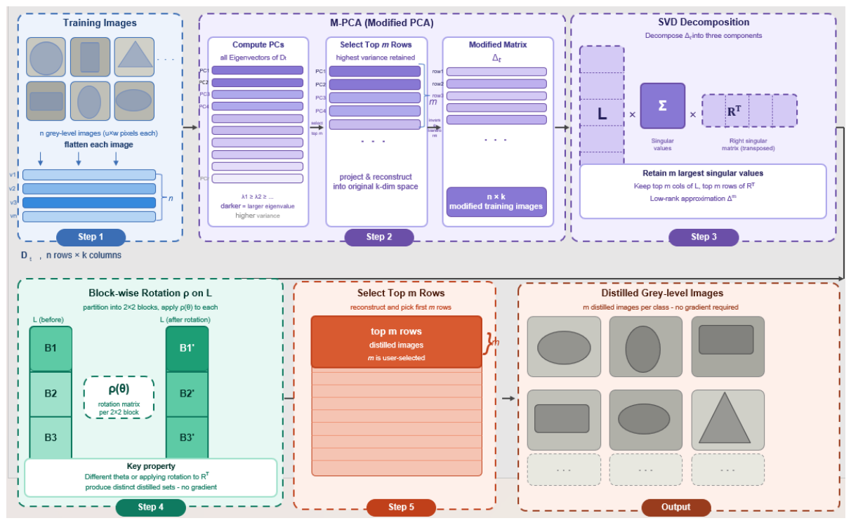
Figure 2.
Randomly selected single original image per class in the top row 1 vs most visually similar distilled image per class using M-PCA-SVD method in row 2. Dataset: Digit-MNIST.
Figure 2.
Randomly selected single original image per class in the top row 1 vs most visually similar distilled image per class using M-PCA-SVD method in row 2. Dataset: Digit-MNIST.
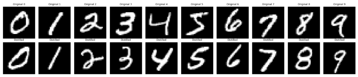
Figure 3.
Randomly selected single original image per class in the top row 1 vs most visually similar distilled image per class using M-PCA-SVD method in row 2. Dataset: Fashion-MNIST.
Figure 3.
Randomly selected single original image per class in the top row 1 vs most visually similar distilled image per class using M-PCA-SVD method in row 2. Dataset: Fashion-MNIST.
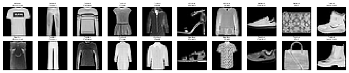
Figure 4.
Randomly selected single original image per class in row 1 vs visually closest single distilled image per class in row 2. Dataset: CIFAR-10.
Figure 4.
Randomly selected single original image per class in row 1 vs visually closest single distilled image per class in row 2. Dataset: CIFAR-10.
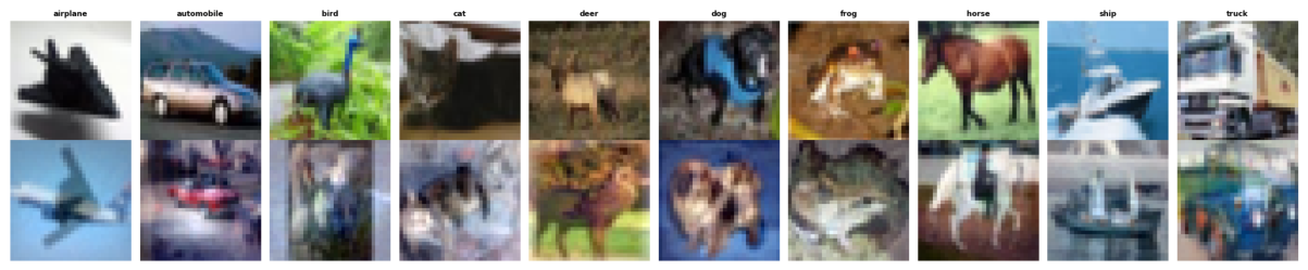
Figure 5.
Randomly selected single original image per class for 10 random classes in row 1 vs distilled image from the same class closest to the original is shown in row 2. Dataset: CIFAR-100.
Figure 5.
Randomly selected single original image per class for 10 random classes in row 1 vs distilled image from the same class closest to the original is shown in row 2. Dataset: CIFAR-100.
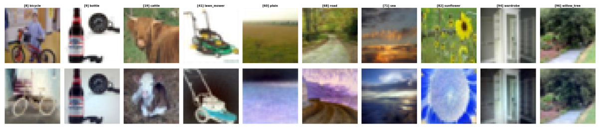
Figure 6.
Four randomly selected original images (left) vs their corresponding QM-PCA-QSVD distilled images (Right). Dataset: BloodMNIST.
Figure 6.
Four randomly selected original images (left) vs their corresponding QM-PCA-QSVD distilled images (Right). Dataset: BloodMNIST.
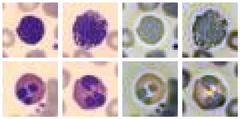
Figure 7.
CIFAR-10 classification results using ResNet50V2 trained on QM-PCA-QSVD distilled images with IPC = 50. (a) Confusion matrix trained for 400 epochs. (b) Training and validation accuracy over 400 epochs.
Figure 7.
CIFAR-10 classification results using ResNet50V2 trained on QM-PCA-QSVD distilled images with IPC = 50. (a) Confusion matrix trained for 400 epochs. (b) Training and validation accuracy over 400 epochs.
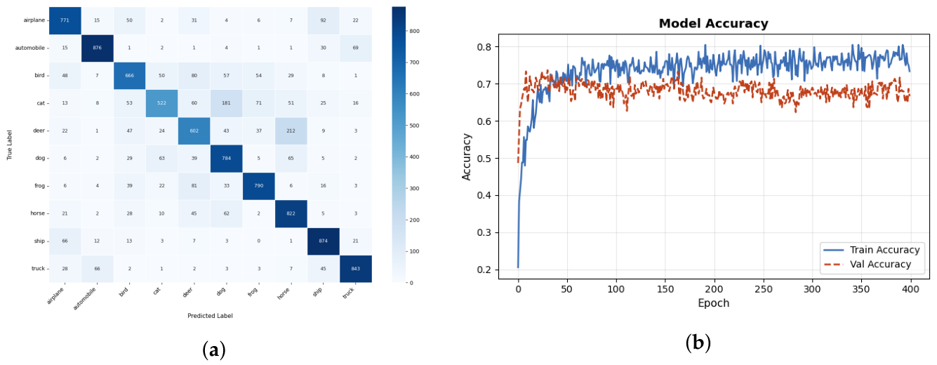

Table 1.
Summary of experimental setup across all datasets.
| Dataset | Network | Distilled IPC | Epochs Tested | Classes |
|---|---|---|---|---|
| Digit-MNIST | Baseline CNN | 10, 20, 50 | 100, 200, 300, 600, 1000 | 10 |
| Fashion-MNIST | Baseline CNN | 10, 20, 50 | 100, 200, 300, 600, 1000 | 10 |
| CIFAR-10 | ResNet50V2 | 10, 50 | 100, 200, 400, 600, 1000 | 10 |
| CIFAR-100 | ResNet50V2 | 10, 50 | 100, 200, 400 | 100 |
| BloodMNIST | Baseline CNN | 10, 50 | 100, 200, 400, 600 | 8 |
Table 2.
Accuracy (in %) of classification of the original test set after training the Baseline NN with distilled images using different IPC and epochs. The highest result in every row is in bold. The symbol — indicates that this experiment was not conducted.
Table 2.
Accuracy (in %) of classification of the original test set after training the Baseline NN with distilled images using different IPC and epochs. The highest result in every row is in bold. The symbol — indicates that this experiment was not conducted.
| Dataset | IPC | Epochs | ||||
|---|---|---|---|---|---|---|
| 100 | 200 | 300 | 600 | 1000 | ||
| 10 | 88.31 | 89.46 | 89.92 | 89.26 | 89.59 | |
| Digit-MNIST | 20 | 92.74 | 93.13 | 93.17 | — | — |
| 50 | 96.89 | 97.43 | 97.68 | 97.12 | 98.01 | |
| 10 | 76.87 | 80.43 | 76.29 | 79.33 | 80.63 | |
| Fashion-MNIST | 20 | 81.55 | 82.22 | 82.69 | — | — |
| 50 | 85.18 | 87.38 | 86.53 | 85.44 | 85.21 | |
Table 3.
Accuracy (in %) comparison when training the Baseline NN with the full original dataset versus distilled images for Digit-MNIST and Fashion-MNIST. The shortest times and highest accuracies are in bold.
Table 3.
Accuracy (in %) comparison when training the Baseline NN with the full original dataset versus distilled images for Digit-MNIST and Fashion-MNIST. The shortest times and highest accuracies are in bold.
| Dataset | IPC | Epochs | Time (sec) | Accuracy (%) |
|---|---|---|---|---|
| Digit-MNIST | 50 (distilled) | 300 | 900 | 97.68 |
| 6000 (original) | 50 | 3656 | 99.54 | |
| Fashion-MNIST | 50 (distilled) | 200 | 1060 | 87.38 |
| 6000 (original) | 50 | 5493 | 92.91 |
Table 4.
Accuracy (in %) of classification of the original test set after training with randomly selected original and distilled images using different images per class and epochs. ResNet50V2 was applied for CIFAR-10 and CIFAR-100; Baseline NN was implemented for BloodMNIST. The highest result in every group is in bold.
Table 4.
Accuracy (in %) of classification of the original test set after training with randomly selected original and distilled images using different images per class and epochs. ResNet50V2 was applied for CIFAR-10 and CIFAR-100; Baseline NN was implemented for BloodMNIST. The highest result in every group is in bold.
| Dataset | IPC | Type | Network | Epochs | ||||
|---|---|---|---|---|---|---|---|---|
| 100 | 200 | 400 | 600 | 1000 | ||||
| CIFAR-10 | 10 | Original | ResNet50V2 | 41.42 | 41.63 | 42.13 | 43.68 | 42.17 |
| Distilled | 72.91 | 73.85 | 73.96 | 73.68 | 73.39 | |||
| CIFAR-10 | 50 | Original | ResNet50V2 | 55.53 | 56.28 | 57.55 | 58.35 | 57.37 |
| Distilled | 73.99 | 74.16 | 75.59 | 74.55 | 74.76 | |||
| CIFAR-100 | 10 | Original | ResNet50V2 | 30.05 | 31.10 | 30.95 | — | — |
| Distilled | 39.98 | 41.27 | 41.95 | — | — | |||
| CIFAR-100 | 50 | Original | ResNet50V2 | 44.34 | 45.47 | 45.15 | — | — |
| Distilled | 51.56 | 55.90 | 56.27 | — | — | |||
| BloodMNIST | 10 | Original | Baseline NN | 65.92 | 67.99 | 73.21 | 70.95 | — |
| Distilled | 70.91 | 72.36 | 73.81 | 72.15 | — | |||
| BloodMNIST | 50 | Original | Baseline NN | 80.33 | 81.44 | 83.98 | 80.88 | — |
| Distilled | 80.83 | 82.39 | 85.47 | 85.30 | — | |||
Table 5.
Accuracy (%) comparison of our methods against state-of-the-art dataset distillation methods. Results are taken from [1]. The last two rows show our results. The bold values indicate the best, and the italic values indicate the second best results in each IPC column.
Table 5.
Accuracy (%) comparison of our methods against state-of-the-art dataset distillation methods. Results are taken from [1]. The last two rows show our results. The bold values indicate the best, and the italic values indicate the second best results in each IPC column.
| Method | Scheme | Digit-MNIST | Fashion-MNIST | CIFAR-10 | CIFAR-100 | ||||
|---|---|---|---|---|---|---|---|---|---|
| IPC=10 | IPC=50 | IPC=10 | IPC=50 | IPC=10 | IPC=50 | IPC=10 | IPC=50 | ||
| Random | — | 95.1 | 97.9 | 73.8 | 82.5 | 26.0 | 43.4 | 14.6 | 30.0 |
| Herding | — | 93.7 | 94.8 | 71.1 | 71.9 | 31.6 | 40.4 | 17.3 | 33.7 |
| DC | GM | 94.7 | 98.8 | 82.3 | 83.6 | 44.9 | 53.9 | 26.6 | 32.1 |
| DSA | GM | 97.8 | 99.2 | 86.6 | 88.7 | 52.1 | 60.6 | 32.4 | 38.6 |
| DCC | GM | — | — | — | — | 54.5 | 64.2 | 33.5 | 39.3 |
| DM | DM | 97.3 | 94.8 | — | — | 48.9 | 63.0 | 29.7 | 43.6 |
| CAFE | DM | 97.5 | 98.9 | 83.0 | 88.2 | 50.9 | 62.3 | 31.5 | 42.9 |
| MTT | TM | 97.3 | 98.5 | 87.2 | 88.3 | 65.3 | 71.6 | 40.1 | 47.7 |
| FTD | TM | — | — | — | — | 66.6 | 73.8 | 43.4 | 50.7 |
| TESLA | TM | — | — | — | — | 66.4 | 72.6 | 41.7 | 47.9 |
| KIP | KRR | 97.5 | 98.3 | 86.8 | 88.0 | 62.7 | 68.6 | 28.3 | — |
| FRePo | KRR | 98.6 | 99.2 | 86.2 | 89.6 | 65.5 | 71.7 | 42.5 | 44.3 |
| RFAD | KRR | 98.5 | 98.8 | 87.0 | 88.8 | 66.3 | 71.1 | 33.0 | — |
| RCIG | KRR | 98.9 | 99.2 | 88.5 | 90.2 | 69.1 | 73.5 | 44.1 | 46.7 |
| IDC* | GM | 98.4 | 99.1 | 86.0 | 86.2 | 67.5 | 74.5 | 44.8 | — |
| DREAM* | GM | 98.6 | 99.2 | 86.4 | 86.8 | 69.4 | 74.8 | 46.8 | 52.6 |
| RTP* | BPTT | 99.3 | 99.4 | 90.0 | 91.2 | 71.2 | 73.6 | 42.9 | — |
| HaBa* | TM | — | — | — | — | 69.9 | 74.0 | 40.2 | 47.0 |
| IDM* | DM | — | — | — | — | 58.6 | 67.5 | 45.1 | 50.0 |
| KFS* | DM | — | — | — | — | 72.0 | 75.0 | 40.0 | 50.6 |
| IADD | PM | — | — | — | — | ||||
| Ours (M-PCA-SVD) | — | 89.92 | 98.01 | 80.63 | 87.38 | — | — | — | — |
| Ours (QM-PCA-QSVD) | — | — | — | — | — | 73.96 | 75.59 | 41.95 | 56.27 |
GM = gradient matching; TM = trajectory matching; DM = distribution matching; KRR = kernel ridge regression; BPTT = backpropagation through time; PM = parameter matching. Methods marked with * use additional components beyond the base scheme. “—” indicates the method was not evaluated on that dataset/IPC in the source paper.
Table 6.
Ablation study on BloodMNIST using the Baseline CNN with 50 distilled images per class (IPC = 50). Accuracy (%) is reported on the original test set. Here WTS = Whole training set. The highest result is in bold.
Table 6.
Ablation study on BloodMNIST using the Baseline CNN with 50 distilled images per class (IPC = 50). Accuracy (%) is reported on the original test set. Here WTS = Whole training set. The highest result is in bold.
| Configuration | Distillation | Network | IPC | Accuracy (%) |
|---|---|---|---|---|
| Original (full dataset) | None | Baseline CNN | 50 | 81.26 |
| M-PCA only | Partial | Baseline CNN | 50 | 84.16 |
| SVM + Grid Search CV [33] | None | EfficientNetV2 | WTS | 76.80 |
| QM-PCA-QSVD + Rotation (Ours) | Full | Baseline CNN | 50 | 85.47 |
Disclaimer/Publisher’s Note: The statements, opinions and data contained in all publications are solely those of the individual author(s) and contributor(s) and not of MDPI and/or the editor(s). MDPI and/or the editor(s) disclaim responsibility for any injury to people or property resulting from any ideas, methods, instructions or products referred to in the content. |
© 2026 by the authors. Licensee MDPI, Basel, Switzerland. This article is an open access article distributed under the terms and conditions of the Creative Commons Attribution (CC BY) license (http://creativecommons.org/licenses/by/4.0/).
Copyright: This open access article is published under a Creative Commons CC BY 4.0 license, which permit the free download, distribution, and reuse, provided that the author and preprint are cited in any reuse.


