Towards an Axiomatic Theory of Geodesics

1. Introduction

Interpolation between points is a fundamental notion throughout mathematics. In Euclidean spaces, interpolation is naturally described by affine combinations: given two points $x,y\in {\mathbb{R}}^n$, the expression

$$x+t(y-x),t\in [0,1],$$

determines the point at parameter t on the line segment joining x and y. In more general geometric settings, however, affine combinations are no longer available. Instead, interpolation is governed by geodesics, which provide distinguished paths connecting points and play a central role in differential geometry, metric geometry and mathematical physics.

A recurring theme in mathematics is the search for algebraic structures capable of capturing geometric phenomena independently of a particular ambient space. Affine spaces, convexity structures and barycentric algebras are classical examples [1] in which geometric behaviour is encoded by algebraic operations. Mobi spaces belong to this tradition. They provide an abstract framework for interpolation through a ternary operation

$$q(x,t,y),$$

interpreted as the point reached at parameter t while travelling from x to y. The axioms satisfied by q are designed to encode the essential compositional properties expected from a parametrized path.

The algebraic foundations of mobi algebras were established in [2]. Mobi spaces were subsequently introduced and studied (see [3] and the references therein). These works revealed strong similarities between the behaviour of geodesics and the axioms of mobi spaces. Nevertheless, a systematic understanding of why geodesic interpolation should produce mobi structures remains incomplete.

The purpose of the present paper is to further develop this connection and to provide additional evidence that mobi spaces may be viewed as an algebraic framework for geodesic interpolation. More broadly, the paper contributes to the programme of extracting algebraic principles from geometric notions of motion and interpolation.

The paper has three main contributions.

First, we reformulate a construction previously introduced in [3]. More precisely, we show that the auxiliary maps involved in that construction can be recovered from a single parametrized map h. This leads to a more intrinsic and conceptually transparent description of the resulting mobi structures.

Second, we establish general conditions under which solutions of second-order differential equations give rise to mobi spaces. The key ingredient is a quadratic homogeneity condition on the acceleration term. This condition is naturally satisfied by geodesic equations arising from Riemannian and pseudo-Riemannian geometry and leads to a fundamental re-parametrization property of geodesic trajectories. This viewpoint naturally separates the ambient space in which the differential equation is defined from the subset on which the resulting mobi structure is constructed.

Third, we present a detailed non-trivial example arising from a metric of non-constant negative curvature. Closed formulas for the corresponding geodesics are obtained, together with the induced mobi structure. This example illustrates concretely how the abstract theory developed in the paper applies to genuine geometric situations beyond the affine case.

Beyond their mathematical interest, these ideas also admit a natural interpretation in physics. From a physical perspective, these results are natural. In classical mechanics and, more prominently, in general relativity, the trajectories of freely moving particles are described by geodesics. Such trajectories arise as solutions of second-order differential equations determined by the underlying geometry, while their parametrizations represent the evolution of the system in time. Viewed in this way, the operation $q(x,t,y)$ may be regarded as an abstract kinematic law assigning to two states all intermediate states of a motion. Mobi spaces therefore provide a geometric-independent language for describing interpolation along trajectories.

The viewpoint adopted in this article suggests that the axioms of a mobi space should not merely be seen as abstract algebraic identities. Rather, they may be interpreted as algebraic manifestations of fundamental properties of geodesic motion, such as re-parametrization, composition of sub-trajectories and uniqueness of interpolation. In this sense, mobi spaces may be regarded as a first step towards an axiomatic theory of geodesics.

The paper is organized as follows. In Section 2 we recall the definitions of mobi algebras and mobi spaces and review some basic examples. In Section 3 we construct an explicit mobi structure from a metric of non-constant negative curvature and derive closed formulas for its geodesics. Section 4 develops a general construction of mobi spaces from a parametrized map. Finally, Section 5 establishes the connection with second-order differential equations and shows how geodesic systems naturally generate mobi spaces. The main result of this paper is Theorem 5.2.

2. Mobi Algebras and Mobi Spaces

We begin by recalling the definition of a mobi algebra, which serves as the algebraic structure governing the parameter t.

Definition 2.1.

A mobi algebra is a system $(A,p,0,\raisebox{1ex}{$1$}\!\left/ \!\raisebox{-1ex}{$2$}\right.,1)$ consisting of a set A, a ternary operation

$$p:A\times A\times A\to A,$$

and distinguished elements 0, $\raisebox{1ex}{$1$}\!\left/ \!\raisebox{-1ex}{$2$}\right.$ and 1, satisfying the following axioms:

• $p(1,\raisebox{1ex}{$1$}\!\left/ \!\raisebox{-1ex}{$2$}\right.,0)=\raisebox{1ex}{$1$}\!\left/ \!\raisebox{-1ex}{$2$}\right.$;
• $p(0,a,1)=a$;
• $p(a,b,a)=a$;
• $p(a,0,b)=a$;
• $p(a,1,b)=b$;
• $p(a,\raisebox{1ex}{$1$}\!\left/ \!\raisebox{-1ex}{$2$}\right.,b_1)=p(a,\raisebox{1ex}{$1$}\!\left/ \!\raisebox{-1ex}{$2$}\right.,b_2)\Rightarrow b_1=b_2$;
• $p(a,p(c_1,c_2,c_3),b)=p(p(a,c_1,b),c_2,p(a,c_3,b))$;
• $p(p(a_1,c,b_1),\raisebox{1ex}{$1$}\!\left/ \!\raisebox{-1ex}{$2$}\right.,p(a_2,c,b_2))=p(p(a_1,\raisebox{1ex}{$1$}\!\left/ \!\raisebox{-1ex}{$2$}\right.,a_2),c,p(b_1,\raisebox{1ex}{$1$}\!\left/ \!\raisebox{-1ex}{$2$}\right.,b_2))$.

Example 2.2.

Let $A=[0,1]$ be the unit interval and define

$$p(a,b,c)=a+b(c-a).$$

Then $(A,p,0,\frac{1}{2},1)$ is a mobi algebra (called the canonical mobi algebra).

Other examples can be found in [2].

We now define mobi spaces.

Definition 2.3.

Let $(A,p,0,\raisebox{1ex}{$1$}\!\left/ \!\raisebox{-1ex}{$2$}\right.,1)$ be a mobi algebra. A mobi space over A is a pair $(X,q)$ where X is a set and

$$q:X\times A\times X\to X$$

is a map satisfying:

(M1) 

$q(x,0,y)=x=q(y,1,x)$;

(M2) 

$q(x,\raisebox{1ex}{$1$}\!\left/ \!\raisebox{-1ex}{$2$}\right.,y_1)=q(x,\raisebox{1ex}{$1$}\!\left/ \!\raisebox{-1ex}{$2$}\right.,y_2)\Rightarrow y_1=y_2$;

(M3) 

$q\left(q\right(x,a,y),b,q(x,c,y\left)\right)=q(x,p(a,b,c),y)$.

Note that the second part of Axiom (M1)

$$q(x,1,y)=y$$

(1)

is deducible from the other axioms. Indeed, using (M3), then (M2) and (M1), and finally (M2), we obtain

$$\begin{array}{cc}\hfill & q(x,p(0,\raisebox{1ex}{$1$}\!\left/ \!\raisebox{-1ex}{$2$}\right.,1),y)=q\left(q\right(x,0,y),\raisebox{1ex}{$1$}\!\left/ \!\raisebox{-1ex}{$2$}\right.,q(x,1,y\left)\right)\hfill \\ \hfill & \iff q(x,\raisebox{1ex}{$1$}\!\left/ \!\raisebox{-1ex}{$2$}\right.,y)=q(x,\raisebox{1ex}{$1$}\!\left/ \!\raisebox{-1ex}{$2$}\right.,q(x,1,y\left)\right)\hfill \\ \hfill & \Rightarrow y=q(x,1,y).\hfill \end{array}$$

Clearly, by the same reason, Axiom (A5), in the definition of a mobi algebra, is also redundant.

At this point, it is worth recalling some basic consequences of the axioms of a mobi space. In particular, it follows from the three axioms of Definition 2.3 that, for all $x\in X$ and all $t\in A$,

$$q(x,t,x)=x.$$

(2)

From the geodesic perspective, this property is natural: the shortest path joining a point to itself is the constant path.

Another important consequence concerns the symmetry of interpolation. If we define

$$\overline{t}=p(1,t,0),$$

(which in the canonical mobi algebra reduces to $\overline{t}=1-t$), then

$$q(y,\overline{t},x)=q(x,t,y).$$

(3)

This reflects a fundamental feature of geodesic motion: travelling from x to y and returning from y to x should follow the same route, traversed in the opposite direction but with the same parametrization speed.

Example 2.4.

Let $X={\mathbb{R}}^n$ and define

$$q(x,t,y)=x+t(y-x).$$

Then $(X,q)$ is a mobi space over the canonical mobi algebra.

Example 2.5.

Let X be a convex subset of a vector space. Then the same formula

$$q(x,t,y)=x+t(y-x)$$

defines a mobi structure. This shows that convex geometry naturally gives rise to mobi spaces.

Example 2.6.

Any mobi algebra is a mobi space over itself.

Example 2.7.

Consider $X=\{z\in \mathbb{C}:|z|=1\}$ as the unit circle and the following operation

$$q(z_1,t,z_2)=\left\{\begin{array}{ccc}{e}^{i\left(arg\left(z_1\right)+targ\left({\displaystyle \frac{z_2}{z_1}}\right)\right)}\hfill & if& arg\left({\displaystyle \frac{z_2}{z_1}}\right)\ne \pi \hfill \\ e^{i\left(arg\left(z_1\right)(1-t)+arg\left(z_2\right)t\right)}\hfill & if& arg\left({\displaystyle \frac{z_2}{z_1}}\right)=\pi \hfill \end{array}\right.,$$

where $arg\left(z\right)$ means the phase angle of the complex number z, considered in the interval $]-\pi ,\pi ]$, as usual. Then $(X,q)$ is a mobi space. This construction has been generalized for the n-sphere, $n\in \mathbb{N}$. Note that, on the unit circle (the 1-sphere), interpolation between two points may be defined along a chosen arc. However, unless one selects a specific arc (e.g., shortest path), the operation $q(x,t,y)$ may fail to verify the axioms of a mobi space, as can be seen clearly in property $\left(\right)$. Moreover, antipodal points must be treated separately: thus for the case $arg\left({\displaystyle \frac{z_2}{z_1}}\right)=\pi$ a choice has been made since there are two shortest paths between the points and only one may be selected.

The previous examples show that mobi spaces include both affine and non-affine situations. In particular, they provide a flexible framework that extends beyond classical affine geometry.

3. Example of Geodesics

In order to motivate the abstract constructions developed later in the paper, we begin with a concrete geometric example. We consider a Riemannian metric of non-constant negative curvature, determine its geodesics explicitly, and show how they naturally induce a mobi structure. This example illustrates the central theme of the paper: the emergence of mobi spaces from geodesic motion.

Consider $U={\mathbb{R}}^{+}\times \mathbb{R}$ endowed with the metric

$$\mathrm{d}{s}^2=\mathrm{d}{x}^2+{\displaystyle \frac{1}{x}}\mathrm{d}{y}^2.$$

(4)

This space has Gaussian curvature (see [4], for instance)

$$K={\displaystyle \frac{-3}{4x^2}},$$

which is negative everywhere and non-constant. From the metric we obtain the non-zero Christoffel symbols (see [5,6], for instance):

$${\Gamma }_{yy}^x={\displaystyle \frac{1}{2x^2}}\mathrm{and}{\Gamma }_{xy}^y={\Gamma }_{yx}^y={\displaystyle \frac{-1}{2x}}.$$

Consequently, the geodesic equations are

$$\begin{array}{cc}\hfill \ddot{x}& =-{\displaystyle \frac{1}{2x^2}}{\dot{y}}^2,\hfill \end{array}$$

(5)

$$\begin{array}{cc}\hfill \ddot{y}& ={\displaystyle \frac{1}{x}}\dot{x}\dot{y},\hfill \end{array}$$

(6)

where $x=x\left(t\right)$, $y=y\left(t\right)$ and the dots denote differentiation with respect to the parameter $t\in \mathbb{R}$.

To solve this system, we first observe that

$$\ddot{y}={\displaystyle \frac{1}{x}}\dot{x}\dot{y}⟺{\displaystyle \frac{1}{x}}\ddot{y}-{\displaystyle \frac{1}{x^2}}\dot{x}\dot{y}=0⟺{\displaystyle \frac{\mathrm{d}}{\mathrm{d}t}}\left({\displaystyle \frac{\dot{y}}{x}}\right)=0.$$

Thus ${\displaystyle \frac{\dot{y}}{x}}$ is constant along every geodesic. Let us denote this constant by L:

$$\dot{y}=Lx.$$

(7)

Substituting this relation into (5), we obtain

$$\ddot{x}=-{\displaystyle \frac{L^2}{2}},$$

whose solution is

$$x\left(t\right)=A+Bt-{\displaystyle \frac{L^2}{4}}{t}^2,$$

(8)

for arbitrary constants $A,B\in \mathbb{R}$.

Using (7) and (8) we get

$$y\left(t\right)=C+ALt+{\displaystyle \frac{BL}{2}}{t}^2-{\displaystyle \frac{L^3}{12}}{t}^3,$$

(9)

where $C\in \mathbb{R}$ is another integration constant.

The velocity along the trajectory is

$$v={\displaystyle \frac{\mathrm{d}s}{\mathrm{d}t}},$$

and, by (4),

$$v^2={\dot{x}}^2+{\displaystyle \frac{1}{x}}{\dot{y}}^2.$$

A direct computation shows that

$$v^2=B^2+A{L}^2,$$

which is constant, as expected for an affinely parametrized geodesic.

The constants may be determined from two points of the geodesic. Suppose that the geodesic passes through $(x_0,y_0)$ at $t=0$ and through $(x_1,y_1)$ at $t=1$. The boundary conditions

$$x\left(0\right)=x_0,x\left(1\right)=x_1,y\left(0\right)=y_0,y\left(1\right)=y_1,$$

imply

$$\begin{array}{cc}\hfill A& =x_0,\hfill \\ \hfill B& =x_1-x_0+{\displaystyle \frac{L^2}{4}},\hfill \\ \hfill C& =y_0,\hfill \end{array}$$

and

$$y_1=y_0+x_{0}L+\left(x_1-x_0+{\displaystyle \frac{L^2}{4}}\right){\displaystyle \frac{L}{2}}-{\displaystyle \frac{L^3}{12}}.$$

After simplification, we obtain

$$L^3+12(x_0+x_1)L+24(y_0-y_1)=0.$$

(10)

The cubic equation (10) admits a unique real solution. Indeed, if

$$f\left(L\right)=L^3+12(x_0+x_1)L+24(y_0-y_1),$$

then

$$f^{\prime }\left(L\right)=3L^2+12(x_0+x_1).$$

Since $x_0,x_1>0$, we have $x_0+x_1>0$ and therefore

$$f^{\prime }\left(L\right)>0$$

for every $L\in \mathbb{R}$. Hence f is strictly increasing and can have at most one real root. On the other hand,

$$\underset{L\to -\infty }{lim}f\left(L\right)=-\infty ,\underset{L\to +\infty }{lim}f\left(L\right)=+\infty ,$$

so, by continuity, f has exactly one real root.

Applying Cardano’s formula to the depressed cubic (10), we obtain

$$\begin{array}{cc}\hfill L& =\sqrt[3]{12(y_1-y_0)+4\sqrt{9{(y_1-y_0)}^2+4{(x_0+x_1)}^3}}\hfill \\ \hfill & +\sqrt[3]{12(y_1-y_0)-4\sqrt{9{(y_1-y_0)}^2+4{(x_0+x_1)}^3}}.\hfill \end{array}$$

(11)

Substituting A, B and C into (8) and (9), while keeping the notation L for the unique solution of (10), we obtain

$$x\left(t\right)=x_0(1-t)+x_{1}t+{\displaystyle \frac{L^2}{4}}t(1-t).$$

(12)

Furthermore,

$$y\left(t\right)=y_0+x_{0}Lt+(x_1-x_0){\displaystyle \frac{L}{2}}{t}^2+{\displaystyle \frac{L^3}{8}}{t}^2-{\displaystyle \frac{L^3}{12}}{t}^3.$$

To obtain a more symmetric expression, we add

$$-{\displaystyle \frac{t}{24}}\left(L^3+12(x_0+x_1)L+24(y_0-y_1)\right),$$

which vanishes by (10), yielding

$$y\left(t\right)=y_0(1-t)+y_{1}t+{\displaystyle \frac{L}{2}}(x_0-x_1)t(1-t)+{\displaystyle \frac{L^3}{24}}t(1-t)(2t-1).$$

(13)

We conclude that for every pair of points in U, say

$$P_0\equiv (x_0,y_0),P_1\equiv (x_1,y_1),$$

and every $t\in [0,1]$, the map

$$q:U\times [0,1]\times U\to U,$$

presented in the example below, gives the position at parameter t of a traveller moving along the unique geodesic joining $P_0$ and $P_1$, with $q(P_0,0,P_1)=P_0$ and $q(P_0,1,P_1)=P_1$.

Example 3.1.

The structure $(U,q)$ is a mobi space over the canonical mobi algebra, with $U={\mathbb{R}}^{+}\times \mathbb{R}$ and

$$\begin{array}{cc}\hfill & q\left((x_0,y_0),t,(x_1,y_1)\right)\hfill \\ \hfill & =(x_0(1-t)+x_{1}t+{\displaystyle \frac{L^2}{4}}t(1-t),\hfill \\ \hfill & y_0(1-t)+y_{1}t+{\displaystyle \frac{L}{2}}(x_0-x_1)t(1-t)+{\displaystyle \frac{L^3}{24}}t(1-t)(2t-1)),\hfill \end{array}$$

(14)

where $L=L(x_0,y_0,x_1,y_1)$ is the unique real solution of (10), explicitly given by (11).

Verifying directly that the operation above satisfies the axioms of a mobi space is a rather cumbersome calculation. Instead, in the next sections we develop a general framework showing that structures arising from geodesic equations naturally satisfy the mobi axioms. In particular, Example 3.1 will later be recovered as a direct consequence of the general construction. This illustrates the guiding principle of the paper: rather than checking the mobi axioms by direct computation, we identify structural features of geodesic equations that force those axioms to hold.

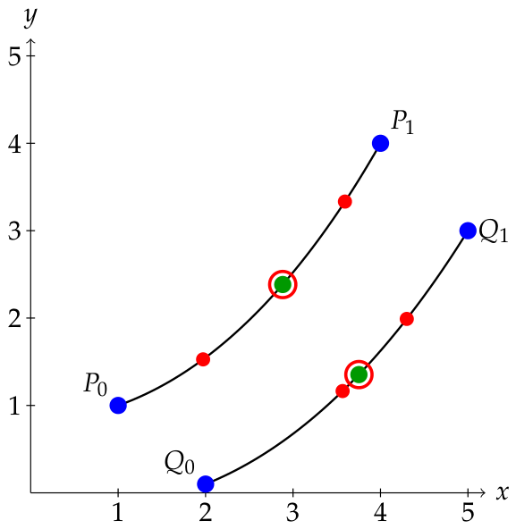
Figure 1 provides a geometric illustration of Axiom c in the context of Example 3.1. Two geodesics are displayed. The first joins the points $P_0=(1,1)$ and $P_1=(4,4)$, while the second joins $Q_0=(2,0.1)$ and $Q_1=(5,3)$.

In each geodesic, the blue points represent the endpoints, the red points correspond to intermediate values of the parameter, and the green point represents the point obtained from the parameter value $p(r,t,s)$. The red circle marks the point obtained by first interpolating between two intermediate points and then applying the parameter t.

For the geodesic joining $P_0$ and $P_1$, the circled point is

$$q\left(q(P_0,0.3,P_1),0.6,q(P_0,0.85,P_1)\right),$$

while the green point is

$$q\left(P_0,p(0.3,0.6,0.85),P_1\right).$$

For the geodesic joining $Q_0$ and $Q_1$, the corresponding points are

$$q\left(q(Q_0,0.5,Q_1),0.25,q(Q_0,0.75,Q_1)\right)$$

and

$$q\left(Q_0,p(0.5,0.25,0.75),Q_1\right).$$

In both cases, the circled point coincides with the green point, showing geometrically the content of Axiom c: interpolation performed within a sub-segment of a geodesic agrees with interpolation computed directly on the whole geodesic through the mobi operation p.

4. Construction of Mobi Spaces via a Given Map h

In [3], a characterization of mobi spaces was presented using several maps (h, $\alpha$ and $\beta$) as part of the given data. In this section we show that the maps $\alpha$ and $\beta$ can be recovered from the parametrized map h itself. This leads to a more intrinsic formulation of the construction, in which the mobi structure is derived solely from h.

Lemma 4.1.

Let $(A,p,0,\raisebox{1ex}{$1$}\!\left/ \!\raisebox{-1ex}{$2$}\right.,1)$ be a mobi algebra and let $\left(V,q_V\right)$ and $\left(T,q_T\right)$ be mobi spaces over that algebra. Consider also the sets $U\subseteq V$ and $I\subseteq T$ closed under the operations $q_V$ and $q_T$, respectively. Now assume that a given map

$$h:V\times T\times V\to V$$

verifies the following conditions: For every $u_1,u_2\in U$ and for every $t_1,t_2\in I$, with $t_1\ne t_2$, there exist a unique solution $\alpha ,\beta \in V$ to the system

$$\left\{\begin{array}{c}{u}_1=h(\alpha ,t_1,\beta )\hfill \\ u_2=h(\alpha ,t_2,\beta )\hfill \end{array}\right.,$$

and $h(\alpha ,q_T(t_1,t,t_2),\beta )\in U$ for every $t\in A$.

Define the map

$$q:(U\times I)\times A\times (U\times I)\to U\times I$$

by

$$q((u_1,t_1),t,(u_2,t_2))=(h(\alpha ,q_T(t_1,t,t_2),\beta ),q_T(t_1,t,t_2))$$

when $t_1\ne t_2$ and, otherwise, by

$$q((u_1,t_1),t,(u_2,t_1))=(q_V(u_1,t,u_2),t_1).$$

Then $(U\times I,q)$ is a mobi space over the mobi algebra $\left(A,p,0,\raisebox{1ex}{$1$}\!\left/ \!\raisebox{-1ex}{$2$}\right.,1\right)$.

In this lemma, the elements $\alpha$ and $\beta$ encode the geometric data from which the interpolation is reconstructed.

Proof. 

The proof consists in verifying the three axioms of a mobi space presented in Definition 2.3.

(M1) Let $(u_1,t_1),(u_2,t_2)\in U\times I$. If $t_1=t_2$, then by definition and using the fact that $(V,q_V)$ is a mobi space, we have:

$$q((u_1,t_1),0,(u_2,t_1))=(q_V(u_1,0,u_2),t_1)=(u_1,t_1)$$

and

$$q((u_1,t_1),1,(u_2,t_1))=(q_V(u_1,1,u_2),t_1)=(u_2,t_1).$$

Assume now that $t_1\ne t_2$ and let $\alpha ,\beta \in V$ be the unique solution of

$$u_1=h(\alpha ,t_1,\beta ),u_2=h(\alpha ,t_2,\beta ).$$

Then

$$q((u_1,t_1),0,(u_2,t_2))=(h(\alpha ,q_T(t_1,0,t_2),\beta ),q_T(t_1,0,t_2)).$$

Since $(T,q_T)$ is a mobi space, $q_T(t_1,0,t_2)=t_1$, and therefore

$$q((u_1,t_1),0,(u_2,t_2))=(h(\alpha ,t_1,\beta ),t_1)=(u_1,t_1).$$

Similarly,

$$q((u_1,t_1),1,(u_2,t_2))=(h(\alpha ,t_2,\beta ),t_2)=(u_2,t_2).$$

Hence axiom (M1) holds.

(M2) Let $(u_1,t_1),(u_2,t_2),(u_3,t_3)\in U\times I$ and assume

$$q((u_1,t_1),\raisebox{1ex}{$1$}\!\left/ \!\raisebox{-1ex}{$2$}\right.,(u_2,t_2))=q((u_1,t_1),\raisebox{1ex}{$1$}\!\left/ \!\raisebox{-1ex}{$2$}\right.,(u_3,t_3)).$$

Comparing second coordinates gives

$$q_T(t_1,\raisebox{1ex}{$1$}\!\left/ \!\raisebox{-1ex}{$2$}\right.,t_2)=q_T(t_1,\raisebox{1ex}{$1$}\!\left/ \!\raisebox{-1ex}{$2$}\right.,t_3).$$

Since $(T,q_T)$ satisfies axiom (M2), $t_2=t_3$. Let $t=t_2=t_3$.

If $t=t_1$, then

$$(q_V(u_1,\raisebox{1ex}{$1$}\!\left/ \!\raisebox{-1ex}{$2$}\right.,u_2),t_1)=(q_V(u_1,\raisebox{1ex}{$1$}\!\left/ \!\raisebox{-1ex}{$2$}\right.,u_3),t_1),$$

hence

$$q_V(u_1,\raisebox{1ex}{$1$}\!\left/ \!\raisebox{-1ex}{$2$}\right.,u_2)=q_V(u_1,\raisebox{1ex}{$1$}\!\left/ \!\raisebox{-1ex}{$2$}\right.,u_3).$$

Using axiom (M2) in $(V,q_V)$ we obtain $u_2=u_3$.

Assume now that $t\ne t_1$. Let $(\alpha ,\beta )$ and $({\alpha }^{\prime },{\beta }^{\prime })$ be the unique solutions associated with $(u_1,u_2)$ and $(u_1,u_3)$ respectively. Equality of first coordinates yields

$$h(\alpha ,q_T(t_1,\raisebox{1ex}{$1$}\!\left/ \!\raisebox{-1ex}{$2$}\right.,t),\beta )=h({\alpha }^{\prime },q_T(t_1,\raisebox{1ex}{$1$}\!\left/ \!\raisebox{-1ex}{$2$}\right.,t),{\beta }^{\prime }).$$

Set $w=h(\alpha ,q_T(t_1,\raisebox{1ex}{$1$}\!\left/ \!\raisebox{-1ex}{$2$}\right.,t),\beta )$. By hypothesis, $w\in U$.

Since

$$h(\alpha ,t_1,\beta )=u_1,h(\alpha ,q_T(t_1,\raisebox{1ex}{$1$}\!\left/ \!\raisebox{-1ex}{$2$}\right.,t),\beta )=w,$$

and likewise

$$h({\alpha }^{\prime },t_1,{\beta }^{\prime })=u_1,h({\alpha }^{\prime },q_T(t_1,\raisebox{1ex}{$1$}\!\left/ \!\raisebox{-1ex}{$2$}\right.,t),{\beta }^{\prime })=w,$$

it follows from the uniqueness assumption that $\alpha ={\alpha }^{\prime }$ and $\beta ={\beta }^{\prime }$. Therefore $u_2=h(\alpha ,t,\beta )=h({\alpha }^{\prime },t,{\beta }^{\prime })=u_3.$ Hence axiom (M2) holds.

(M3) Let $(u_1,t_1),(u_2,t_2)\in U\times I$ and $r,s,t\in A$. We have to prove that $Q_1=Q_2$, where

$$\begin{array}{cc}\hfill Q_1& =q\left((u_1,t_1),p(r,t,s),(u_2,t_2)\right);\hfill \\ \hfill Q_2& =q\left(q((u_1,t_1),r,(u_2,t_2)),t,q((u_1,t_1),s,(u_2,t_2))\right).\hfill \end{array}$$

To simplify the presentation of the proof, the following notations are used:

$$t_r=q_T(t_1,r,t_2)\mathrm{and}{t}_s=q_T(t_1,s,t_2).$$

Three cases have to be analysed.

1.

If $t_1=t_2$, then

$$\begin{array}{cc}\hfill Q_1& =\left(q_V(u_1,p(r,t,s),u_2),t_1\right)\hfill \\ \hfill Q_2& =q\left((q_V(u_1,r,u_2),t_1),t,(q_V(u_1,s,u_2),t_1)\right)\hfill \\ \hfill & =\left(q_V(q_V(u_1,r,u_2),t,q_V(u_1,s,u_2)),t_1\right).\hfill \end{array}$$

First coordinates are equal because $(V,q_V)$ is a mobi space. Hence $Q_1=Q_2$.

2.

If $t_1\ne t_2$ and $t_r\ne t_s$, then

$$\begin{array}{cc}\hfill Q_1& =\left(h(\alpha ,q_T(t_1,p(r,t,s),t_2),\beta ),q_T(t_1,p(r,t,s),t_2)\right)\hfill \\ \hfill & =(h(\alpha ,q_T(t_r,t,t_s),\beta ),q_T(t_r,t,t_s))\hfill \\ \hfill Q_2& =q\left(\left(h(\alpha ,t_r,\beta ),t_r\right),t,\left(h(\alpha ,t_s,\beta ),t_s\right)\right)\hfill \\ \hfill & =\left(h(\tilde{\alpha },q_T(t_r,t,t_s),\tilde{\beta }),q_T(t_r,t,t_s)\right).\hfill \end{array}$$

where the pairs $(\alpha ,\beta )$ and $(\tilde{\alpha },\tilde{\beta })$ verify the following systems:

$$\left\{\begin{array}{c}h(\alpha ,t_1,\beta )=u_1\hfill \\ h(\alpha ,t_2,\beta )=u_2\hfill \end{array}\right.,\left\{\begin{array}{c}h(\tilde{\alpha },t_r,\tilde{\beta })=h(\alpha ,t_r,\beta )\hfill \\ h(\tilde{\alpha },t_s,\tilde{\beta })=h(\alpha ,t_s,\beta )\hfill \end{array}\right..$$

Calling ${\chi }_r\equiv h(\alpha ,t_r,\beta )$ and ${\chi }_s\equiv h(\alpha ,t_s,\beta )$, the same pairs also verify the following systems:

$$\left\{\begin{array}{c}h(\alpha ,t_r,\beta )={\chi }_r\hfill \\ h(\alpha ,t_s,\beta )={\chi }_s\hfill \end{array}\right.,\left\{\begin{array}{c}h(\tilde{\alpha },t_r,\tilde{\beta })={\chi }_r\hfill \\ h(\tilde{\alpha },t_s,\tilde{\beta })={\chi }_s\hfill \end{array}\right..$$

By hypothesis, there is a unique solution to each of these systems and therefore $\tilde{\alpha }=\alpha$ and $\tilde{\beta }=\beta$. Consequently $Q_1=Q_2$.

3.

If $t_1\ne t_2$ and $t_r=t_s$, then

$$\begin{array}{cc}\hfill Q_1& =(h(\alpha ,q_T(t_r,t,t_s),\beta ),q_T(t_r,t,t_s))\hfill \\ \hfill & =\left(h(\alpha ,t_r,\beta ),t_r\right)\hfill \\ \hfill Q_2& =q\left(\left(h(\alpha ,t_r,\beta ),t_r\right),t,\left(h(\alpha ,t_s,\beta ),t_s\right)\right)\hfill \\ \hfill & =\left(q_V(h(\alpha ,t_r,\beta ),t,h(\alpha ,t_s,\beta )),t_r\right),\mathrm{with}{t}_r=t_s\hfill \\ \hfill & =\left(h(\alpha ,t_r,\beta ),t_r\right).\hfill \end{array}$$

And again $Q_1=Q_2$.

Therefore axiom (M3) holds.

Thus $(U\times I,q)$ is a mobi space. □

Example 4.2.

Consider $U=V={\mathbb{R}}^n,T=\mathbb{R},I={\mathbb{R}}^{+}$ and $A=[0,1]$. Consider also the canonical mobi operations in each set:

$$\begin{array}{ccc}\hfill q_V(x,t,y)& =& x+t(y-x)\hfill \\ \hfill q_T(t_1,t,t_2)& =& t_1+t(t_2-t_1)\hfill \\ \hfill p(a,t,b)& =& a+t(b-a)\hfill \end{array}$$

There is no doubt that I is closed under $q_T$. Let h be given by

$$h(x,t,y)=x+t^{2}y.$$

For every $u_1,u_2\in {\mathbb{R}}^n$ and every $t_1,t_2\in {\mathbb{R}}^{+}$, with $t_1\ne t_2$, there is a unique $\alpha \in {\mathbb{R}}^n$ and a unique $\beta \in {\mathbb{R}}^n$ such that

$$\left\{\begin{array}{c}{u}_1=\alpha +t_1^2\beta \hfill \\ u_2=\alpha +t_2^2\beta \hfill \end{array}\right.,$$

namely: $\alpha ={\displaystyle \frac{t_2^2{u}_1-t_1^2{u}_2}{t_2^2-t_1^2}}$ and $\beta ={\displaystyle \frac{u_2-u_1}{t_2^2-t_1^2}}$. Now we can define the mobi operation

$$q:({\mathbb{R}}^n\times {\mathbb{R}}^{+})\times [0,1]\times ({\mathbb{R}}^n\times {\mathbb{R}}^{+})\to ({\mathbb{R}}^n\times {\mathbb{R}}^{+})$$

by

$$q((u_1,t_1),t,(u_2,t_2))=(\alpha +{\left(q_T(t_1,t,t_2)\right)}^2\beta ,q_T(t_1,t,t_2))$$

when $t_1\ne t_2$ and, otherwise, by

$$q((u_1,t_1),t,(u_2,t_1))=(q_V(u_1,t,u_2),t_1).$$

In summary, we get a new mobi space $({\mathbb{R}}^n\times {\mathbb{R}}^{+},q)$ over the canonical mobi algebra $([0,1],p,0,\frac{1}{2},1)$ with:

$$\begin{array}{cc}\hfill & q((u_1,t_1),t,(u_2,t_2))\hfill \\ \hfill & =\left\{\begin{array}{ccc}\left(u_1+{\displaystyle \frac{2t{t}_1+t^2(t_2-t_1)}{t_1+t_2}}(u_2-u_1),t_1+t(t_2-t_1)\right)\hfill & if& t_1\ne t_2\hfill \\ \left(u_1+t(u_2-u_1),t_1\right)\hfill & if& t_1=t_2\hfill \end{array}\right..\hfill \end{array}$$

In fact, in this example, since $t_1,t_2\in {\mathbb{R}}^{+}$, we don’t need a piecewise function and can simply write

$$\begin{array}{cc}\hfill & q((u_1,t_1),t,(u_2,t_2))\hfill \\ \hfill & =\left(u_1+{\displaystyle \frac{2t{t}_1+t^2(t_2-t_1)}{t_1+t_2}}(u_2-u_1),t_1+t(t_2-t_1)\right).\hfill \end{array}$$

This example shows that adding a time coordinate may transform a non-mobi parametrization into a genuine mobi structure on a larger space.

The previous Lemma shows that it is relatively straightforward to construct a mobi space if, instead of a given set U, we add an extra dimension in order to end up with a mobi space over $U\times I$. But, we may be interested in constructing a mobi space over the set U alone. In particular, we may want to decide at which parameters $t_1$ and $t_2$ the points $u_1$ and $u_2$ are reached (for instance $t_1=0$ and $t_2=1$). This does not work with the previous example where $h(x,t,y)=x+t^{2}y$. Indeed, if we impose

$$\left\{\begin{array}{c}{u}_1=h(\alpha ,0,\beta )\hfill \\ u_2=h(\alpha ,1,\beta )\hfill \end{array}\right.,$$

we end up with $\alpha =u_1$ and $\beta =u_2-u_1$. This leads to a map $q(u_1,t,u_2)=u_1+t^2(u_2-u_1)$ that does not verify the Axiom c of a mobi space. On the contrary, if we start with $h(x,t,y)=x+ty$, $U=V={\mathbb{R}}^n$ and $A=[0,1]$ and solve the same system at $t_1=0$ and $t_2=1$, we end up with $q(u_1,t,u_2)=u_1+t(u_2-u_1)$ which is a mobi map and, in fact, we recover the standard affine canonical structure. This shows that there exist maps h that could imply a mobi structure directly on U without an extra dimension, but this comes at the cost of extra conditions on h as described in the next proposition.

For an easier understanding of the next proposition, it may be useful to recall that a mobi algebra is a mobi space over itself and hence a particular case is that of $(T,q_T)$ being a mobi algebra with $T\supseteq A$. In this case, considering $t_1=0$ and $t_2=1$ as working model we get $q_T(t_1,t,t_2)=t$

Proposition 4.3.

Let $(A,p,0,\raisebox{1ex}{$1$}\!\left/ \!\raisebox{-1ex}{$2$}\right.,1)$ be a mobi algebra and $(T,q_T)$ a mobi space over that algebra. Consider a set V and a subset $U\subseteq V$. Assume that, for fixed $t_1,t_2\in T$ with $t_1\ne t_2$, a given map

$$h:V\times T\times V\to V$$

verifies the following conditions.

(a) 

For every $u_1,u_2\in U$, there exist a unique solution $\alpha ,\beta \in V$ to the system

$$\left\{\begin{array}{c}{u}_1=h(\alpha ,t_1,\beta )\hfill \\ u_2=h(\alpha ,t_2,\beta )\hfill \end{array}\right.,$$

and $h(\alpha ,q_T(t_1,t,t_2),\beta )\in U$ for every $t\in A$. Since $t_1$ and $t_2$ are fixed, we can write

$$\alpha =\alpha (u_1,u_2)\mathrm{and}\beta =\beta (u_1,u_2).$$

(b) 

For all $x,y,y^{\prime }\in V$,

$$\begin{array}{cc}\hfill & h(x,q_T(t_1,\raisebox{1ex}{$1$}\!\left/ \!\raisebox{-1ex}{$2$}\right.,t_2),y)=h(x,q_T(t_1,\raisebox{1ex}{$1$}\!\left/ \!\raisebox{-1ex}{$2$}\right.,t_2),y^{\prime })\hfill \\ \hfill & ⟹h(x,t_2,y)=h(x,t_2,y^{\prime }).\hfill \end{array}$$

(c) 

For all $x,y\in V$ and $r,s,t\in A$, if

$$h(x,q_T(t_1,r,t_2),y)\mathrm{and}h(x,q_T(t_1,s,t_2),y)\mathrm{belong}\mathrm{to}\mathrm{U}$$

then:

$$\begin{array}{cc}\hfill & h(x,q_T(t_1,p(r,t,s),t_2),y)\hfill \\ \hfill & =h(\alpha (h(x,q_T(t_1,r,t_2),y),h(x,q_T(t_1,s,t_2),y)),q_T(t_1,t,t_2),\hfill \\ \hfill & \beta (h(x,q_T(t_1,r,t_2),y),h(x,q_T(t_1,s,t_2),y))).\hfill \end{array}$$

Define $q:U\times A\times U\to U$ by

$$q(u_1,t,u_2)=h(\alpha (u_1,u_2),q_T(t_1,t,t_2),\beta (u_1,u_2)).$$

Then $(U,q)$ is a mobi space over the mobi algebra $(A,p,0,\raisebox{1ex}{$1$}\!\left/ \!\raisebox{-1ex}{$2$}\right.,1)$.

Among the assumptions of Proposition 4.3, condition $\left(c\right)$ is the least immediate. Although it may appear artificial at first sight, Section 5 shows that it is in fact a natural re-parametrization identity satisfied by trajectories arising from suitable second-order differential equations.

Proof. 

Again, we have to verify the three axioms of a mobi space presented in Definition 2.3.

(M1) We need to consider any two elements in U, say u and v. Under the hypothesis (a), we have guaranteed the existence of unique functions $\alpha (u,v)\in V$ and $\beta (u,v)\in V$ such that $u=h(\alpha (u,v),t_1,\beta (u,v))$ and $v=h(\alpha (u,v),t_2,\beta (u,v))$. Consequently, using a on $q_T$,

$$q(u,0,v)=h(\alpha (u,v),t_1,\beta (u,v))=u,$$

and

$$q(u,1,v)=h(\alpha (u,v),t_2,\beta (u,v))=v,$$

which proves a for q.

(M2) In order to prove b, let us suppose $u,v,v^{\prime }\in U$ are such that

$$q(u,\raisebox{1ex}{$1$}\!\left/ \!\raisebox{-1ex}{$2$}\right.,v)=q(u,\raisebox{1ex}{$1$}\!\left/ \!\raisebox{-1ex}{$2$}\right.,v^{\prime })$$

which is the same as

$$h(\alpha (u,v),q_T(t_1,\raisebox{1ex}{$1$}\!\left/ \!\raisebox{-1ex}{$2$}\right.,t_2),\beta (u,v))=h(\alpha (u,v^{\prime }),q_T(t_1,\raisebox{1ex}{$1$}\!\left/ \!\raisebox{-1ex}{$2$}\right.,t_2),\beta (u,v^{\prime })).$$

From here, hypothesis (b) implies

$$h(\alpha (u,v),t_2,\beta (u,v))=h(\alpha (u,v^{\prime }),t_2,\beta (u,v^{\prime }))$$

which, by definition of q, is the same as

$$q(u,1,v)=q(u,1,v^{\prime })$$

and we make use of axiom a, already proved, to get the desired equality $v=v^{\prime }$.

(M3) Finally, to prove c, let us take any $u,v\in U$ and $r,s,t\in A$. Define $x=\alpha (u,v)$ and $y=\beta (u,v)$. Note that $h(x,q_T(t_1,r,t_2),y)\in U$ and $h(x,q_T(t_1,s,t_2),y)\in U$, by $\left(a\right)$. Hence, by definition of q, condition (c) is precisely axiom c. □

Example 4.4.

Let U be a convex subset of $V={\mathbb{R}}^n$, $A=T=[0,1]$, $\left(A,p,0,\frac{1}{2},1\right)$ the canonical algebra and $q_T=p$. Consider a function $F:V\to V$ whose restriction to the subset U is injective and denote by $G:Im\left(F{|}_U\right)\to U$ the inverse of ${F|}_U$. Consider also the map $h(x,t,y)=F(x+ty)$. With the choices $t_1=0$ and $t_2=1$, it is straightforward to check that h verifies the hypotheses of Proposition 4.3, with $\alpha (u,v)=G\left(u\right)$ and $\beta (u,v)=G\left(v\right)-G\left(u\right)$. Consequently, the operation

$$q(u,t,v)=F\left(G\left(u\right)(1-t)+G\left(v\right)t\right)$$

defines a mobi structure on $Im\left(F{|}_U\right)$, obtained by transporting the standard affine interpolation through the map F.

However, in general, the conditions of Proposition 4.3 are not easy to check directly. The main purpose of the next section is to show that these apparently technical conditions are in fact natural consequences of the structure of geodesic equations like the ones presented in Section 3.

5. Mobi Spaces from Geodesics

The purpose of this section is to show that the hypotheses of Proposition 4.3 are not ad hoc. In fact, they arise naturally from the structure of geodesic equations.

It is important to distinguish between the ambient space on which the differential equation is defined and the subset on which the resulting mobi structure is constructed. In general, solutions of a differential equation may exist in a larger space V, while the mobi operation is only required on a subset $U\subseteq V$. Proposition 4.3 reflects this distinction: the parametrized trajectories are described in the ambient space, but only those trajectories that remain in U are used to define the mobi structure.

Geodesics may be considered in various kinds of spaces (e.g., [7,8]). For example, geodesics are well defined in discrete sets like graphs or trees, which also lead to mobi spaces. However, in this section, we will focus on Riemannian manifolds (or pseudo-Riemannian manifolds) (see [9,10] for instance). Let $X\subseteq {\mathbb{R}}^n$ be an open set endowed with a Riemannian metric, and let ${\Gamma }_{ij}^k$ be the associated Christoffel symbols. Then, the geodesic equations are

$${\ddot{x}}^k\left(t\right)=-\sum _{i,j}{\Gamma }_{ij}^k\left(x\left(t\right)\right){\dot{x}}^i\left(t\right){\dot{x}}^j\left(t\right),$$

(15)

where $x\left(t\right)$ represents the vector with components $x^k\left(t\right)$. If $h(x_0,t,v_0)$ denotes the unique solution with initial conditions $x\left(0\right)=x_0$, $\dot{x}\left(0\right)=v_0$, this may result in a mobi space by applying Proposition 4.3. The following theorem sets up the framework for this. A fundamental observation is that (15) can be written in the form $\ddot{x}=g(x,v)$, with $v=\dot{x}$ and, most importantly, the function g has the following homogeneous property relative to the v-variable: $g(x,\lambda v)={\lambda }^{2}g(x,v)$, with $\lambda \in \mathbb{R}$.

Lemma 5.1.

Let U be a subset of a real vector space V.

Consider a map $g:V\times V\to V$ satisfying

$$g(x,\lambda v)={\lambda }^{2}g(x,v)$$

(16)

for all $x,v\in V$ and $\lambda \in \mathbb{R}$.

Assume that, for every $(u,v)\in V\times V$, the initial value problem

$$f^{\prime \prime }\left(t\right)=g(f\left(t\right),f^{\prime }\left(t\right)),f\left(0\right)=u,f^{\prime }\left(0\right)=v$$

(17)

admits a unique solution $f\left(t\right)\in V$ defined for all $t\in \mathbb{R}$. Denote this solution by $h(u,t,v)$ with $h:V\times \mathbb{R}\times V\to V.$ Then, for every $u,v\in V$, the following property holds

$$h(u,r+t(s-r),v)=h(h(u,r,v),t,(s-r)h^{\prime }(u,r,v)),$$

(18)

where $h^{\prime }$ denotes the first derivative of h with respect to its second argument.

The significance of Lemma 5.1 is that it provides exactly the kind of composition property required in Proposition 4.3. It shows that a segment of a solution trajectory may be viewed as an entire trajectory with suitably modified initial data. Consequently, interpolation along a trajectory is compatible with subdivision and re-parametrization.

Proof. 

We will use $h^{\prime \prime }$ for the second derivative of h with respect to its second argument. Consider any $u,v\in V$ and any $r,s,t\in \mathbb{R}$. Since h is the solution of the initial value problem (17), we have that

• $h(u,0,v)=u$
• $h^{\prime }(u,0,v)=v$
• $h^{\prime \prime }(u,t,v)=g(h(u,t,v),h^{\prime }(u,t,v)).$

We can define:

• $f_1\left(t\right)=h(u,r+t(s-r),v)$;
• $f_2\left(t\right)=h(h(u,r,v),t,(s-r)h^{\prime }(u,r,v))$

We easily find that:

$$\begin{array}{cc}\hfill f_1\left(0\right)& =h(u,r,v)\hfill \\ \hfill f_1^{\prime }\left(0\right)& =(s-r)h^{\prime }(u,r,v)\hfill \\ \hfill f_1^{\prime \prime }\left(t\right)& ={(s-r)}^2{h}^{\prime \prime }(u,r+t(s-r),v)\hfill \\ \hfill & ={(s-r)}^{2}g(h(u,r+t(s-r),v),h^{\prime }(u,r+t(s-r),v))\hfill \\ \hfill & =g(h(u,r+t(s-r),v),(s-r)h^{\prime }(u,r+t(s-r),v))\hfill \\ \hfill & =g(f_1\left(t\right),f_1^{\prime }\left(t\right)),\hfill \end{array}$$

where (16) was used in the penultimate equality.

In a similar way, we find that:

$$\begin{array}{cc}\hfill f_2\left(0\right)& =h(u,r,v)\hfill \\ \hfill f_2^{\prime }\left(0\right)& =(s-r)h^{\prime }(u,r,v)\hfill \\ \hfill f_2^{\prime \prime }\left(t\right)& =h^{\prime \prime }(h(u,r,v),t,(s-r)h^{\prime }(u,r,v))\hfill \\ \hfill & =g(h(h(u,r,v),t,(s-r)h^{\prime }(u,r,v)),\hfill \\ \hfill & h^{\prime }(h(u,r,v),t,(s-r)h^{\prime }(u,r,v)))\hfill \\ \hfill & =g(f_2\left(t\right),f_2^{\prime }\left(t\right)).\hfill \end{array}$$

Therefore $f_1$ and $f_2$ satisfy the same initial value problem (17), with $u=h(u,r,v)$ and $v=(s-r)h^{\prime }(u,r,v)$, which by hypothesis has a unique solution. Hence $f_1=f_2$ which proves (18) and consequently the lemma. □

A particular case of (18), when $r=0$, reads

$$h(u,ts,v)=h(u,t,sv).$$

This shows that changing the speed of the motion simply amounts to a re-parametrization of the same trajectory.

Theorem 5.2.

Let $(A,p,0,\frac{1}{2},1)$ be the canonical mobi algebra (see Example 2.2), and let U be a subset of a real vector space V.

Consider a map $g:V\times V\to V$ satisfying

$$g(x,\lambda v)={\lambda }^{2}g(x,v)$$

for all $x,v\in V$ and $\lambda \in \mathbb{R}$.

Assume that, for every $(u,v)\in V\times V$, the initial value problem

$$f^{\prime \prime }\left(t\right)=g(f\left(t\right),f^{\prime }\left(t\right)),f\left(0\right)=u,f^{\prime }\left(0\right)=v$$

admits a unique solution $f\left(t\right)=h(u,t,v)$ defined for all $t\in \mathbb{R}$.

Assume moreover that

(i)

for every $x,y\in U$ there exists a unique vector $\beta (x,y)\in V$ such that

$$h(x,1,\beta (x,y\left)\right)=y;$$

(ii)

for every $x,y\in U$ and every $t\in A$,

$$h(x,t,\beta (x,y\left)\right)\in U.$$

Define $q:U\times A\times U\to U$ by

$$q(x,t,y)=h(x,t,\beta (x,y\left)\right).$$

Then $(U,q)$ is a mobi space over the canonical mobi algebra.

Proof. 

We verify the axioms of a mobi space directly.

(M1) For every $x,y\in U$,

$$q(x,0,y)=h(x,0,\beta (x,y\left)\right)=x,$$

since $h(x,0,v)=x$ for every $v\in V$. Moreover,

$$q(x,1,y)=h(x,1,\beta (x,y\left)\right)=y$$

by hypothesis $\left(i\right)$.

(M2) Assume that

$$q\left(x,{\displaystyle \frac{1}{2}},y_1\right)=q\left(x,{\displaystyle \frac{1}{2}},y_2\right).$$

Then

$$h\left(x,{\displaystyle \frac{1}{2}},\beta (x,y_1)\right)=h\left(x,{\displaystyle \frac{1}{2}},\beta (x,y_2)\right).$$

By the particular case of Lemma 5.1 where $r=0$,

$$h(u,ts,v)=h(u,t,sv),$$

and therefore

$$h\left(x,{\displaystyle \frac{1}{2}},v\right)=h\left(x,1,{\displaystyle \frac{1}{2}}v\right).$$

Hence

$$h\left(x,1,{\displaystyle \frac{1}{2}}\beta (x,y_1)\right)=h\left(x,1,{\displaystyle \frac{1}{2}}\beta (x,y_2)\right).$$

By the uniqueness in hypothesis $\left(i\right)$, it follows that

$${\displaystyle \frac{1}{2}}\beta (x,y_1)={\displaystyle \frac{1}{2}}\beta (x,y_2),$$

and therefore

$$\beta (x,y_1)=\beta (x,y_2).$$

Consequently,

$$y_1=h(x,1,\beta (x,y_1))=h(x,1,\beta (x,y_2))=y_2.$$

(M3) Let $x,y\in U$ and $r,s,t\in A$. Put

$$v=\beta (x,y).$$

By Lemma 5.1,

$$h(x,p(r,t,s),v)=h\left(h(x,r,v),t,(s-r)h^{\prime }(x,r,v)\right).$$

Evaluating the same identity at $t=1$ gives

$$h(x,s,v)=h\left(h(x,r,v),1,(s-r)h^{\prime }(x,r,v)\right).$$

Since hypothesis $\left(ii\right)$ ensures that

$$h(x,r,v),h(x,s,v)\in U,$$

the expression

$$\beta \left(h(x,r,v),h(x,s,v)\right)$$

is well defined. By the uniqueness in hypothesis $\left(i\right)$,

$$\beta \left(h(x,r,v),h(x,s,v)\right)=(s-r)h^{\prime }(x,r,v).$$

Substituting into the first identity yields

$$h(x,p(r,t,s),v)=h\left(h(x,r,v),t,\beta \left(h(x,r,v),h(x,s,v)\right)\right).$$

Using the definition of q, we obtain

$$q(x,p(r,t,s),y)=q\left(q(x,r,y),t,q(x,s,y)\right),$$

which is precisely axiom (M3).

Therefore $(U,q)$ is a mobi space. Alternatively, this result follows from Proposition 4.3 once conditions $\left(a\right)$, $\left(b\right)$ and $\left(c\right)$ are verified using Lemma 5.1. □

Theorem 5.2 shows that the mobi axioms arise naturally from three fundamental ingredients: existence and uniqueness of solutions, quadratic homogeneity of the acceleration term, and uniqueness of the velocity sending one point to another. Consequently, Proposition 4.3 may be viewed as an abstract formulation of the uniqueness and re-parametrization properties underlying geodesic motion.

Example 5.3.

We now present explicit maps g, h and β associated with the geodesic structure described in Section 3. The sets are $A=[0,1]$, $V={\mathbb{R}}^2$ and $U={\mathbb{R}}^{+}\times \mathbb{R}$. When $x_1\ne 0$, the map g is obtained directly from Equations (5) and ():

$$g((x_1,x_2),(v_1,v_2))=\left(-{\displaystyle \frac{1}{2x_1^2}}{v}_2^2,{\displaystyle \frac{1}{x_1}}{v}_1{v}_2\right).$$

The map g is defined on $V={\mathbb{R}}^2$ by extending the formula in an arbitrary way along the line $x_1=0$, preserving the homogeneity condition (16), as for instance $g((0,x_2),(v_1,v_2))=0$. The values of g on that line are irrelevant for the present construction, since all trajectories under consideration remain in U. To find the maps h and β to which Theorem 5.2 can apply, the variables $u=(u_1,u_2),v=(v_1,v_2)\in V$ must be carefully chosen among the four integration variables $A,B,C$ and L because the equalities $h(u,0,v)=u$ and $h^{\prime }(u,0,v)=v$ must hold. Comparing (8) and (9) with these requirements, we obtain the choice $u=(A,C)$ and $v=(B,AL)$, with which we get:

$$\begin{array}{cc}\hfill h((u_1,u_2),t,(v_1,v_2))=(& u_1+v_{1}t-{\displaystyle \frac{v_2^2}{4u_1^2}}{t}^2,\hfill \\ & u_2+v_{2}t+{\displaystyle \frac{v_1{v}_2}{2u_1}}{t}^2-{\displaystyle \frac{v_2^3}{12u_1^3}}{t}^3)\hfill \end{array}$$

and

$$\beta ((x_0,x_1),(y_0,y_1))=((x_1-x_0)+{\displaystyle \frac{L^2}{4}},x_{0}L),$$

where L is given by (11). It is straightforward to check that

$$h^{\prime \prime }((u_1,u_2),t,(v_1,v_2))=g(h((u_1,u_2),t,(v_1,v_2)),h^{\prime }((u_1,u_2),t,(v_1,v_2))).$$

The uniqueness of β follows from the uniqueness of the real solution L of Equation (10), together with the formulas for A, B and C obtained in Section 3. Indeed, once L is determined, the corresponding values of A, B and C are uniquely determined by the boundary data. Moreover, Equations (12) and (13) show that $h(x,t,\beta (x,y\left)\right)\in U$ for every $t\in [0,1]$. Hence hypotheses (i) and (ii) of Theorem 5.2 are satisfied. Applying Theorem 5.2 to these data, we conclude that the operation obtained from

$$q(x,t,y)=h(x,t,\beta (x,y\left)\right)$$

is a mobi operation on U. A direct computation shows that this operation is precisely the map described in Example 3.1. Therefore Example 3.1 is recovered as a special case of the general theory developed above.

Theorem 5.2 may be interpreted as a converse to the usual geometric viewpoint. Rather than defining geodesics from a geometric structure and then studying interpolation, we obtain an interpolation algebra directly from the differential equation governing the trajectories.

6. Conclusions

The main goal of this paper was to further clarify the relationship between mobi spaces and geodesic interpolation. Starting from the geometric intuition that a geodesic determines intermediate states between two points, we developed an algebraic framework in which this interpolation is encoded by the axioms of a mobi space.

A first contribution was the reformulation of a previous construction of mobi spaces in terms of a single parametrized map h. This provides a more intrinsic description of the construction and shows that the auxiliary data used in earlier approaches can be recovered directly from the parametrization.

Our second contribution was the establishment of a general mechanism through which solutions of second-order differential equations generate mobi spaces. The crucial ingredient is a quadratic homogeneity property of the acceleration term, which yields a natural re-parametrization law. Since geodesic equations arising from Riemannian and pseudo-Riemannian geometry satisfy this property, the resulting framework applies to a broad class of geometric situations.

Finally, we worked out explicitly a non-trivial example associated with a metric of non-constant negative curvature. Besides illustrating the theory, this example shows that mobi structures naturally arise beyond the affine and constant-curvature settings considered in earlier work.

Taken together, these results strengthen the interpretation of mobi spaces as algebraic models of geodesic interpolation and provide further evidence that they may serve as a useful foundation for an axiomatic theory of geodesics.

References

- Romanowska, A.; Smith, J. D. H. Modes. In World Scientific Lecture Notes in Mathematics; World Scientific, 2002. [Google Scholar]
- Fatelo, J. P.; Martins-Ferreira, N. Mobi algebra as an abstraction to the unit interval and its comparison to rings. Commun. Algebra 2019, 47(3), 1197–1214. [Google Scholar] [CrossRef]
- Fatelo, J. P.; Martins-Ferreira, N. An algebraic approach to geodesics via mobi spaces. Axioms 2026, 15, 352. [Google Scholar] [CrossRef]
- Pressley, A. Elementary Differential Geometry, 2nd Edition; Springer, 2010. [Google Scholar]
- do Carmo, M. P. Riemannian Geometry; Birkhäuser, 1992. [Google Scholar]
- Ryder, L. Introduction to general relativity; Cambridge University Press, 2009. [Google Scholar]
- Bridson, M. R.; Haefliger, A. Metric Spaces of Non-Positive Curvature; Springer, 1999. [Google Scholar]
- Chiswell, I. M. Introduction to Λ-trees; World Scientific, 2001. [Google Scholar]
- Boothby, W. M. An Introduction to Differentiable Manifolds and Riemannian Geometry; Academic Press, 2003. [Google Scholar]
- Jost, J. Riemannian geometry and Geometric Analysis, 7th Edition; Springer, 2017. [Google Scholar]
Figure 1.
Two geodesics of Example 3.1 illustrating Axiom (M3).
Disclaimer/Publisher’s Note: The statements, opinions and data contained in all publications are solely those of the individual author(s) and contributor(s) and not of MDPI and/or the editor(s). MDPI and/or the editor(s) disclaim responsibility for any injury to people or property resulting from any ideas, methods, instructions or products referred to in the content. |
© 2026 by the authors. Licensee MDPI, Basel, Switzerland. This article is an open access article distributed under the terms and conditions of the Creative Commons Attribution (CC BY) license (http://creativecommons.org/licenses/by/4.0/).
Copyright: This open access article is published under a Creative Commons CC BY 4.0 license, which permit the free download, distribution, and reuse, provided that the author and preprint are cited in any reuse.