
Submitted:
08 July 2026
Posted:
08 July 2026
You are already at the latest version
Abstract
Rock physics model provides an essential theoretical tool to quantify the impacts of reservoir physical parameters (porosity, water saturation, etc.) on seismic elastic properties including P- wave velocity and S-wave velocity. As a core module for deriving physical properties through joint well-seismic inversion, rock physics modeling accuracy directly determines the reliability of reservoir property prediction. Simultaneous characterization of pores and oriented fractures is required to refine modeling precision, yet the resulting excessive model parameters severely limit applications to field seismic data. To address the critical issue of applying pore and fracture anisotropic rock physics models to azimuthal seismic interpretation, this work decouples pores and oriented fractures during modeling. We postulate that pore variations control the model’s isotropic elastic properties, whereas oriented fracture characteristics dominate anisotropic parameters. Well-log data are utilized to invert key modeling parameters (matrix mineral elastic moduli, fracture porosity, etc.) for model correction. The corrected rock physics model is further coupled with the Rüger reflectivity equation to analyze how porosity and fracture azimuth alter seismic reflection coefficients and synthetic seismic records. The presented anisotropic rock physics correction method via parameter inversion greatly elevates modeling accuracy. Rock-physics-based analysis of azimuthal seismic reflection shows promising prospects for widespread use in fractured reservoir characterization.
Keywords:
rock physics model
; azimuthal seismic reflection
; anisotropic
; pore
; fracture
1. Introduction
Rock physics models act as an essential bridge connecting seismic elastic parameters with reservoir physical parameters. Generally, conventional rock physics modeling can be implemented via three standard procedures. Firstly, different minerals are homogenized to determine the elastic moduli of equivalent solid matrices. Secondly, pores and fractures are introduced into the solid matrices to calculate the elastic moduli of dry rock. Thirdly, various pore fluids are mixed and injected into dry rock to acquire the elastic moduli of fluid-saturated rocks. Among the whole modeling process, equivalent medium theory lays a theoretical foundation and plays a decisive role.
Equivalent medium theory is the fundamental theoretical support for rock physics modeling. According to whether the pore geometry effect is taken into consideration, existing equivalent medium models can be classified into two categories: models ignoring pore shape effects (i.e., bound models) and models considering pore shape effects (i.e., self-consistent models). Bound models were first proposed in the 1920s. Among them, the upper bound of elastic modulus for mixed mineral compositions pro-posed by Voigt [1] and the lower bound proposed by Reuss [2] are two most classical theoretical frameworks. Apart from verifying the rationality of newly established rock physics models, the average value of Voigt and Reuss bounds can be adopted to calculate the average elastic modulus of minerals and further estimate the elastic properties of equivalent solid matrices. This widely used averaging method is defined as the Voigt-Reuss-Hill (VRH) average theory [3].
When calculating the elastic moduli of dry rock, it is generally assumed that pores within the solid matrix dominate the isotropic elastic properties of media. Three classic and representative isotropic equivalent medium models that account for pores and their morphological effects are widely adopted in rock physics research. Specifically, the Kuster-Toksöz (K-T) model is derived based on the first-order wave scattering theory [4]. The self-consistent approximation (SCA) model requires no predefined background medium and treats all mineral components equally without priority [5]. Different from the SCA model, the differential effective medium (DEM) model distinguishes primary and secondary mineral components according to the sequence of mineral addition during modeling [6].
In contrast, oriented fractures will induce anisotropic elastic characteristics of rock media during the calculation of elastic moduli for dry rock frameworks. For anisotropic media with ellipsoidal inclusions, Hudson established a classic rock physics model applicable to thin penny-shaped fractures and first proposed the definition of fracture density [7]. Nevertheless, the original Hudson model suffers from obvious limitations, particularly its poor performance for fractures with small aspect ratios. Subsequent theoretical derivations have removed unreasonable assumptions of the original model and greatly extended its applicable scope [8]. On the other hand, when fractures are simplified as vertically oriented infinite planar cracks, the fractured rock medium can be equivalent to HTI (Horizontal Transverse Isotropy) medium, and the Schoenberg theory suitable for slender fractures has been developed correspondingly [9]. With continuous improvement, the Schoenberg theory can further characterize the variation of elastic parameters caused by changing fracture aspect ratios and has achieved favorable application performance in field reservoir evaluation. By integrating linear slip theory with matrix pore-based equivalent medium theory, a novel pore-fracture medium model with a single set of vertically aligned fractures is constructed, which can quantitatively analyze the respective contributions of pores and fractures to rock elastic properties. Currently, rock physics theories coupling pores and fractures have been well developed, and such integrated models have been widely applied to cope with complex actual geological conditions [10,11,12,13,14,15].
On the basis of previous research, we develop a novel rock physics model considering both pore shape and the azimuth of oriented fractures. To improve the accuracy of the established model, model correction is performed via inversion for elastic moduli of minerals and oriented fracture parameters, which realizes a fine matching between the theoretical model and logging data. Thereafter, an inversion objective function is constructed based on the corrected rock physics model to quantitatively predict the azimuth of oriented fractures. Ultimately, combined with the Rüger approximate equation for seismic re-flection coefficients [16], the proposed rock physics model is adopted to theoretically clarify the response mechanism of reservoir physical parameters to seismic reflection characteristics.
2. Materials and Methods
2.1. Rock Physics Model with Pores and Oriented Fractures
Rock physics modeling is to establish a functional relationship between seismic elastic parameters and reservoir physical parameters. Rock physics modeling mainly consists of three steps: Mix minerals to calculate the equivalent elastic modulus of the matrix; Introduce pores and fractures to compute the elastic modulus of the dry rock; Incorporate fluids to obtain the elastic parameters of fluid-saturated rock. The detailed modeling workflow is as follows:
-
The Voigt-Reuss-Hill average method [3] is adopted to mix minerals and calculate the equivalent elastic moduli of the rock matrix. It is assumed that the minerals of sandstone consist of sandy minerals and clay minerals. The expressions for equivalent bulk modulus, shear modulus and density of rock matrix are given as follows:In Equations (1–3): denotes clay content, denotes sand fraction. We assume , meaning the rock matrix only contains two mineral components: sandy minerals and clay minerals. and are the bulk modulus and shear modulus of sandy minerals, respectively, and is the density of sandy minerals; and are the bulk modulus and shear modulus of clay minerals, respectively, and is the density of clay minerals. In addition, in Equation. (1) and in Equation (2) represent the Voigt upper bounds of the bulk modulus and shear modulus of the rock matrix, while and stand for the Reuss lower bounds of the rock matrix bulk modulus and shear modulus, respectively;
- The equivalent bulk modulus and density of fluids are calculated using the Wood equation [17]:where denotes water saturation, denotes gas saturation. We assume , meaning the fluid is a mixture of water and natural gas; and are the bulk moduli of water and gas, respectively; and are the densities of water and gas, respectively; is the equivalent bulk modulus of mixed pore fluids, and is the equivalent density of mixed pore fluids;
- The SCA model [6] is adopted to incorporate pores with variable pore aspect ratios into the equivalent rock matrix:where and denote the bulk modulus and shear modulus of rock after embedding fluid-saturated pores, respectively; represents matrix porosity, and denotes the aspect ratio of pores; and are geometric coefficients accounting for variations in pore aspect ratios;
- The Schoenberg model [9] is applied to introduce fractures with variable strike azimuths into the rock containing pores. First, the Lamé constant is calculated using the bulk modulus and shear modulus of the pore-bearing rock:
Assuming the oriented fractures are vertical with variable strike azimuths, the stiffness matrix of the rock physical model accounting for pore geometries and strike angles of aligned fractures can be expressed as:
where and represent the stiffness matrix of the isotropic background rock medium containing only pores and the stiffness perturbation induced by oriented fractures, respectively:
The expressions for the oriented fracture parameters and in Equation (11) are given as follows:
where denotes the aspect ratio of oriented fractures, whose value is generally much smaller than that of pores. is the squared ratio of S-wave velocity to P-wave velocity of the rock with pores, represents the oriented fracture density, and the expressions for and are written as:
where denotes the porosity of oriented fractures, whose magnitude is generally far smaller than pore porosity. Assuming the strike azimuth of oriented fractures is , the stiffness matrix of fluid-saturated rock is written as:
In Equation (16):
Given the stiffness matrix of fluid-saturated rock, the P-wave velocity and S-wave velocity , as well as three HTI anisotropy parameters [16] , and , can be calculated therefrom. In addition, the bulk density is obtained via weighted averaging, are written as:
Thus far, the construction of the rock physical model accounting for pores and oriented fractures has been completed. The mapping relationship between the anisotropic elastic parameters of rock and physical parameters is written as:
2.2. Stochastic Inversion Algorithm with Variable Sampling Space
Given logging data containing anisotropic elastic parameters (P-wave and S-wave velocities, density, three anisotropy parameters) and three physical parameters (porosity, clay content and water saturation), we aim to invert unknown parameters including pore aspect ratio and fracture strike azimuth. To address this complicated nonlinear multi-parameter inversion issue, a variable sampling space stochastic inversion method [18] is introduced. This algorithm is applied in two stages to correct the rock physics model for well log datasets.
Figure 1 shows the flowchart of the stochastic inversion algorithm with variable sampling space, and its detailed procedures are described as follows:
- Firstly, assign the prior probability density function, then generate N random sample points following this distribution;
- During every iteration, we retain the top samples with the smallest objective function values. Assuming these samples obey Gaussian statistics, we compute their new mean and variance ;
- Resample N sample points based on the updated Gaussian distribution, and then launch the next iteration. This procedure is repeated until the algorithm converges.
Figure 1 assumes lower objective function values represent smaller calculation errors. If higher objective function values correspond to smaller errors, samples are sorted descendingly. Input parameters of the inversion algorithm: sample count N, maximum iterations, shrinkage factor ( must be integer), amplification factor . Factor extracts well-fitted samples for statistics. Factor enlarges variance to expand sample space and enrich candidate cases in resampling.
3. Results
The logging dataset contains P-wave velocity, S-wave velocity, bulk density, three anisotropy parameters (, and ), and three physical parameters (porosity, clay content, and water saturation). Taking Well A as an example, Figure 2 illustrates its full logging profiles, encompassing nine elastic and physical parameters in total.
3.1. Inversion-Based Correction of Rock Physics Model
From the principle of rock physics modeling, the rock physics model behaves isotropically when the effect of oriented fractures is not incorporated. In reservoir conditions, the porosity of oriented fractures is generally much smaller than the total porosity of the rock. Under the assumption that fracture porosity is far lower than total porosity, P-wave velocity, S-wave velocity, density, porosity, clay content and water saturation are combined with the isotropic component of the rock-physical model (i.e., the isotropic rock physics model that only accounts for pores) to invert the elastic moduli of minerals for model correction.
In this step, the three anisotropy parameters are temporarily excluded, and the other six logging parameters are treated as known inputs. A stochastic inversion algorithm with variable sampling space is utilized to invert mineral elastic moduli and correct the isotropic component of the rock physics model. Taking logging-derived porosity, clay content and water saturation as inputs, Figure 3 compares the elastic parameters computed from the corrected isotropic rock physics model with the elastic parameters acquired from well logging measurements.
In Figure 3, the red curves denote logging data, and the blue curves stand for P-wave velocity, S-wave velocity and density calculated from the corrected isotropic component of the rock physics model. The correction is realized by inverting mineral elastic moduli using a stochastic inversion algorithm with variable sampling space, where logging porosity, clay content and water saturation serve as input variables. Density is calculated via Equation (20). The equivalent densities of sand and clay minerals are predefined and . Pore fluids are treated as a binary mixture of natural gas and water, where the shear modulus of fluid is zero. The bulk modulus and density of natural gas and , as well as the bulk modulus and density of water and , are specified. Using logging data to invert the elastic moduli of minerals, the objective function for correcting the isotropic component of the rock physics model is established as follows:
where and denote the measured P- and S- wave velocities from well logging, respectively; and are the P- and S-wave velocities calculated by the isotropic component of the rock physics model, which are written as:
In the objective function expressed by Equation (25), the variables are the elastic moduli of minerals, namely the parameters to be inverted. It is assumed that the prior probability density distribution of mineral elastic moduli follows a Gaussian distribution. The mean values of the initial model for mineral elastic moduli are referenced to the rock physics handbook [17]: the initial mean of bulk modulus for sand minerals is 37.00 GPa with a variance of 4.00; the initial mean of shear modulus for sand minerals is 44.00 Gpa with a variance of 4.00; the initial mean of bulk modulus for clay minerals is 21.00 Gpa with a variance of 4.00; the initial mean of shear modulus for clay minerals is 7.00 Gpa with a variance of 4.00. The stochastic inversion algorithm with variable sampling space is utilized to invert the elastic moduli of minerals. The preset algorithm parameters are set as: the number of sampling points N=500, maximum iteration number of 10, shrinkage coefficient aqa=0.3 and expansion coefficient apa=1.2. The bulk modulus of sand minerals , shear modulus of sand minerals , bulk modulus of clay minerals and shear modulus of clay minerals are acquired after inversion. The inverted elastic moduli of minerals are substituted into Equations (1) and (2) to establish the inversion-corrected rock physics model. The elastic parameters of the isotropic component of the corrected rock physics model in Figure 3 are calculated subsequently. Then, error analysis is conducted between the simulated elastic parameters obtained from the corrected model and the logging elastic parameters, and the corresponding analysis results are presented in Figure 4.
It can be seen from Figure 4 that the maximum frequency of errors of both P- and S-wave velocity appears around zero, which indicates that the inversion process for mineral elastic moduli based on the inversion algorithm with variable sampling space is feasible. At this point, the correction for the isotropic component of the rock physics model is completed.
Taking P-wave velocity, S-wave velocity, density and three anisotropic parameters as known parameters, five physical parameters including pore porosity, pore aspect ratio, oriented fracture porosity, azimuth of oriented fractures and clay content are inverted by using the rock physics model with corrected isotropic component. The inversion results of physical parameters are shown in Figure 5.
Figure 5e compares the inverted clay content with logging-measured clay content, and Figure 5f compares the sum of inverted pore porosity and oriented fracture porosity with logging total porosity. The red curves represent logging data, while the blue curves denote inversion results. It can be seen that both inverted clay content and total porosity match well with logging data. The correlation coefficient of clay content is 0.66, and that of porosity is 0.78, both indicating strong correlations.
Figure 6 shows the comparison between logging data and P-wave velocity, S-wave velocity as well as three anisotropic parameters calculated by the rock physics model using physical parameters inverted from Figure 5.
It can be observed from Figure 6 that the errors of P-wave and S-wave velocities are lower than those of anisotropic parameters. This demonstrates that the inversion accuracy of physical parameters for the isotropic component of the rock physics model (including pore porosity, pore aspect ratio and clay content) is higher than that of physical parameters for the anisotropic component (including aligned fracture porosity and aligned fracture strike azimuth). Meanwhile, it also proves that the inversion of anisotropic physical parameters is more difficult than that of isotropic physical parameters.
3.2. Azimuthal Seismic Reflection Characteristics Analysis Based on Rock Physics
The rock physics model is further combined with the AVAZ reflection coefficient equation to analyze the influences of variations in physical parameters on reflection coefficients and synthetic seismic records. In horizontally transverse isotropic (HTI) media, the reflection coefficient varies with incident angle and azimuth angle [16].
In Equation (28) IP stands for P-wave impedance, denotes shear modulus, refers to the included angle between the symmetry axis of the medium and the principal direction (generally ), represents the seismic wave incident angle, and is the observation azimuth angle. The reflection coefficients at different azimuth angles under fixed incident angles are shown in Figure 7a, and the reflection coefficients at different incident angles under fixed azimuth angles are shown in Figure 7b:
Figure 7 presents the reflection coefficients at different azimuth angles and incident angles calculated from the logging data in Figure 2 based on Equation (28). It can be observed that the variation of incident angles exerts a more significant influence on reflection coefficients compared with azimuth angles. This phenomenon is caused by the small absolute values of anisotropic parameters derived from logging data. As shown in Figure 2 and Figure 6, the absolute values of anisotropic parameters are relatively small, approximately equal to 0.1.
Since the overall time-domain range of reflection coefficients calculated from time-depth converted logging data in Figure 7 is less than 30 ms, a Ricker wavelet with a dominant frequency of 160 Hz and a sampling interval of 1 ms is adopted to convolve with reflection coefficients to highlight seismic events. Figure 8a shows synthetic seismic records at incident angles of 0°, 15° and 30° when the azimuth angle is 0°; Figure 8b shows synthetic seismic records at incident angles of 0°, 15° and 30° when the azimuth angle is 45°; Figure 8c shows synthetic seismic records at incident angles of 0°, 15° and 30° when the azimuth angle is 90°. Nevertheless, the dominant frequency of actual seismic data can hardly reach 160 Hz. To fit the actual field conditions better, another Ricker wavelet with a dominant frequency of 40 Hz and a sampling interval of 1 ms is used for convolution. Figure 8d displays synthetic seismic records at incident angles of 0°, 15° and 30° under the azimuth angle of 0°; Figure 8e displays synthetic seismic records at incident angles of 0°, 15° and 30° under the azimuth angle of 45°; Figure 8f displays synthetic seismic records at incident angles of 0°, 15° and 30° under the azimuth angle of 90°.
It can be observed from Figure 8a that when the azimuth angle is fixed at 0°, the incident angle imposes an obvious effect on synthetic seismic records, and the amplitude of synthetic seismic records gradually decreases with the increase of incident angle. Figure 8c presents a similar variation law for an azimuth angle of 90°, consistent with that for azimuth angles of 0° and 45°, namely the seismic amplitude declines gradually as the incident angle rises. However, the influence of incident angle on synthetic seismic records is weaker at the azimuth angle of 90° than that at 0° and 45°. Similarly, Figure 8d indicates that incident angle changes have a prominent impact on synthetic seismic records at the azimuth angle of 0°, while Figure 8f shows a fairly weak impact of incident angle at the azimuth angle of 90°. Overall, within the azimuth angle range from 0° to 90°, the smaller the azimuth angle, the more significant the influence of incident angle variation on synthetic seismic records generated by wavelets with different dominant frequencies.
Since the oriented fracture porosity is generally much lower than the pore porosity, the total porosity can be approximately regarded as pore porosity when ignoring the influence of oriented fracture porosity. Under this assumption, we change the pore porosity values and analyzes the effects of pore porosity variations on synthetic seismic records at different incident angles by adopting the inversion-corrected rock physics model. It can be seen from Figure 2 that the total porosity presents a low magnitude, with most values less than 0.1. Keeping other physical parameters unchanged, we discuss the influence of increasing pore porosity on synthetic seismic records at incident angles of 0°, 15° and 30° under the azimuth angle of 0°, and the relevant results are displayed in Figure 9. Consistent with the processing workflow for Figure 8, a Ricker wavelet with a dominant frequency of 160 Hz and a sampling interval of 1 ms is used for convolution of reflection coefficients to highlight seismic events. Figure 9a shows synthetic seismic records at different incident angles calculated by taking the total logging porosity as matrix porosity; Figure 9b,c show synthetic seismic records at different incident angles with assumed matrix porosity of 0.2 and 0.3, respectively. Furthermore, another Ricker wavelet with a dominant frequency of 40 Hz and a sampling interval of 1 ms is adopted for convolution. The impacts of rising matrix porosity on synthetic seismic records at incident angles of 0°, 15° and 30° under the azimuth angle of 0° are illustrated in Figure 9d, Figure 9e and Figure 9f, respectively. Specifically, Figure 9d presents synthetic seismic records at different incident angles calculated using total logging porosity and the 40 Hz dominant-frequency wavelet; Figure 9e corresponds to synthetic seismic records with matrix porosity of 0.2 and the 40 Hz wavelet; Figure 9f corresponds to synthetic seismic records with matrix porosity of 0.3 and the 40 Hz wavelet.
It can be observed from Figure 9 that the amplitudes of synthetic seismic records at different incident angles all increase with the rising pore porosity. The variation law of seismic events obtained from the 160 Hz dominant-frequency wavelet is basically consistent with that from the 40 Hz dominant-frequency wavelet. Compared with synthetic seismic records generated by the 160 Hz wavelet, the records based on the 40 Hz wavelet show a more prominent phenomenon: when the pore porosity is at a low level, the change of pore porosity has a greater influence on seismic amplitude. Specifically, the difference of seismic events between Figure 9e,e is more significant than that between Figure 9e,f.
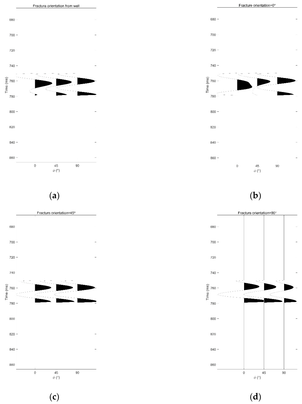
This section further analyzes the influence of azimuth variation of oriented fractures on synthetic seismic records with different observation azimuth angles. Given that the oriented fracture porosity is assumed to be much smaller than pore porosity during rock physics modeling, the variation of fracture porosity has limited significance for seismic response analysis. In contrast, the change of fracture azimuth imposes a more prominent impact on synthetic seismic records with different observation azimuth angles. In addition, the fractures established in the rock physics model are set to have variable strike azimuths and vertical dips. Theoretically, the variation of fracture azimuth has no influence on seismic waves under vertical incidence (incident angle = 0°), and such influence becomes more significant as the incident angle increases. Therefore, the incident angle is fixed at 30° to explore the effects of varying fracture azimuths on synthetic seismic records at observation azimuth angles of 0°, 45° and 90°, and the corresponding results are shown in Figure 10. To highlight the response difference of seismic events caused by fracture azimuth variation, a Ricker wavelet with a dominant frequency of 40 Hz and a sampling interval of 1 ms is adopted for reflection coefficient convolution. Figure 10a shows synthetic seismic records at different observation azimuth angles calculated based on the predicted fracture azimuth from logging data in Figure 5; Figure 10b, Figure 10c and Figure 10d display synthetic seismic records at different observation azimuth angles with assumed fracture strike azimuths of 0°, 45° and 90°, respectively.
As illustrated in Figure 10, the azimuth of fractures exerts dual effects on synthetic seismic records: it not only modulates the amplitude characteristics of seismic responses, but also changes the spatial position of seismic events. Specifically, fractures with an azimuth of 0° impose a significant influence on synthetic seismic records corresponding to different observation azimuths. Among all tested fracture schemes, the synthetic seismic record established under the fracture azimuth of 45° achieves the optimal matching effect with well logging data, with only slight deviations existing in the position of seismic events. In comparison with other fracture azimuths involved in this study, the most remarkable difference of the 90° strike azimuth lies in its unique amplitude variation law: the amplitude of seismic events presents a continuous decreasing trend with the increase of observation azimuth.
4. Discussion
In the process of rock physics modeling, the influences of pores and oriented fractures on the elastic properties of geological media are considered separately. Variations in pore porosity affect the isotropic elastic parameters of the media, while changes in oriented fractures dominate the variations of anisotropic elastic parameters. The purpose of separately introducing pores and oriented fractures during rock physics modeling is to eliminate the influence of oriented fractures conveniently when correcting the rock physics model via inverted mineral elastic moduli, which can be realized by directly removing the fracture addition procedure from the original rock physics model.
When combining the corrected rock physics model with the approximate reflection coefficient equation of HTI media to investigate how variations in oriented fracture azimuth alter synthetic seismic records, a seismic incident angle of 30° is adopted in numerical simulations under the controlled-variable principle. In this framework, the azimuth of fractures serves as the sole variable, and the rock physics model assumes vertical dip for oriented fractures. At an incident angle of 0° (vertical incidence), changes in fracture azimuth impose no observable effect on seismic responses. In general, the influence of fracture azimuth becomes more pronounced as the incident angle increases. To prominently characterize the azimuthal effect of oriented fractures on synthetic seismic records, we perform simulations at a relatively large incident angle of 30°. This result further implies that high-quality azimuthal seismic data with large incident angles are essential prerequisites for the prediction of steeply dipping fractures.
5. Conclusions
We focus on the critical issue of applying anisotropic rock physics models to analyze logging data and azimuthal seismic data. A rock physics model suitable for logging data is established, and a stochastic inversion algorithm with variable sampling space is pro-posed to invert the parameters of the anisotropic rock physics model for model correction. To improve the adaptability of the rock physics model to actual well logging data, the stochastic inversion algorithm is adopted to invert key parameters required for rock phys-ics modeling, including the elastic moduli of minerals and fracture porosity, so as to cor-rect the rock physics model for better matching with logging measurements. The corrected rock physics model is employed to construct an objective function for petrophysical pa-rameter inversion. The inverted petrophysical parameters are compared with well logging data to verify their accuracy. By combining the corrected rock physics model with the ap-proximate azimuthal reflection coefficient equation and adjusting petrophysical parame-ter values, this study further analyzes the influences of variations in pore porosity and azimuth of oriented fractures on synthetic seismic records. We provide a theoretical foun-dation for monitoring pores and fractures in anisotropic reservoirs containing vertically dipping fractures with arbitrary azimuths using azimuthal seismic data. Simulating the effects of petrophysical parameter variations on synthetic seismic records via theoretical rock physics models enables theoretical characterization of how reservoir petrophysical property changes impact time-lapse seismic data at different azimuths during energy production, which lays a theoretical foundation for monitoring energy exploitation with time-lapse seismic technology.
Author Contributions
Conceptualization, Yipeng Gu; methodology, Yipeng Gu; software, Yipeng Gu and Na Huang; validation, Maoshan Chen, Chen Xu and Ruidong Han; formal analysis, Maoshan Chen; inves-tigation, Yipeng Gu; resources, Yipeng Gu; data curation, Chen Xu; writing—original draft preparation, Yipeng Gu and Na Wu; writing—review and editing, Yipeng Gu; visualization, Yipeng Gu; supervision, Yipeng Gu; project administration, Yipeng Gu; funding acquisition, Yipeng Gu. All authors have read and agreed to the published version of the manuscript.
Funding
This research was funded by 2025 Annual Daily Research Funding Grant for Postdoctoral Re-searchers of Hebei Province.
Data Availability Statement
The raw data supporting the conclusions of this article will be made available by the authors on request.
Acknowledgments
The authors sincerely thank the journal editors and anonymous reviewers for their constructive comments and valuable suggestions to improve the quality of this manuscript.
Conflicts of Interest
The authors declare no conflicts of interest.
Abbreviations
The following abbreviations are used in this manuscript:
| HTI | Horizontal Transverse Isotropy |
References
- Reuss, A. Berechnung der Fließgrenze von Mischkristallen auf Grund der Plastizitätsbedingung für Einkristalle. Z. Angew. Math. Und Mech. 1929, 9(1), 49–58. [Google Scholar] [CrossRef]
- Hashin, Z.; Shtrikman, S. A variational approach to the theory of the elastic behaviour of polycrystals. J. Mech. Phys. Solids 1962, 10(4), 343–352. [Google Scholar] [CrossRef]
- Hill, R. Elastic properties of reinforced solids: some theoretical principles. J. Mech. Phys. Solids 1963, 11(5), 357–372. [Google Scholar] [CrossRef]
- Kuster, G. T.; Toksöz, M. N. Velocity and attenuation of seismic waves in two-phase media: Part I. Theoretical formulations. Geophysics 1974, 39(5), 587–606. [Google Scholar] [CrossRef]
- Berryman, J. G. Long-wavelength propagation in composite elastic media. J. Acoust. Soc. Am. 1980, 68(B), 1809–1831. [Google Scholar] [CrossRef]
- Berryman, J. G. Single-scattering approximations for coefficients in Biot’s equations of poroelasticity. J. Acoust. Soc. Am. 1992, 91(2), 551–571. [Google Scholar] [CrossRef]
- Huson, J. A. Wave speeds and attenuation of elastic waves in material containing cracks. Geophys. J. Int. 1981, 64(1), 133–150. [Google Scholar] [CrossRef]
- Cheng, C. H. Crack models for a transversely isotropic medium. J. Geophys. Res. Solid Earth 1993, 98(B1), 675–684. [Google Scholar] [CrossRef]
- Schoenberg, M. Elastic wave behavior across linear slip interfaces. J. Acoust. Soc. Am. 1980, 68(5), 1516–1521. [Google Scholar] [CrossRef]
- Chapman, M. Frequency-dependent anisotropy due to meso-scale fractures in the presence of equant porosity. Geophys. Prospect. 2003, 51(5), 369–379. [Google Scholar] [CrossRef]
- Phansakorn, K.; Mark, S.; et al. Integrated seismic and well log data conditioning for seismic inversion. Lead. Edge 2026, 1070–485X. [Google Scholar]
- Vashisth, D.; Lessard, R.; Mukerji, T. Prestack and poststack seismic inversion using quantum computing. Geophysics 2026, 91(4), R163–R173. [Google Scholar]
- Jiayuan, H.; Mukerji, T. Joint rock physics inversion and basin modeling for comprehensive source rock characterization. Lead. Edge 2026, 45(5), 391–400. [Google Scholar] [CrossRef]
- Russell, B.; Goodway, B.; Avseth, P. Poroelasticity and rock-physics templates. Interpretation 2025, 13(1), T139–T152. [Google Scholar]
- Rui, Y.; Huaizhen, C. A novel rock-physics model of organic-rich shale considering maturation influence. Geophysics 2024, 89(4), MR223–MR236. [Google Scholar] [CrossRef]
- Rüger, A. Reflection coefficients and azimuthal AVO analysis in anisotropic media. In SEG; Geophysical Monograph Series, 2002; p. 10. [Google Scholar]
- Mavko, G.; Mukerji, T.; Dvorkin, J. The rock physics handbook; Cambridge university press, 2020. [Google Scholar]
- Gu, Y.; Yin, X.; Zhang, J.; et al. Prediction of reservoir physical parameters based on adaptive step size stochastic inversion. Geoenergy Sci. Eng. 2023, 223, 211455. [Google Scholar] [CrossRef]
Figure 1.
Flowchart of the stochastic inversion algorithm with variable sampling space.
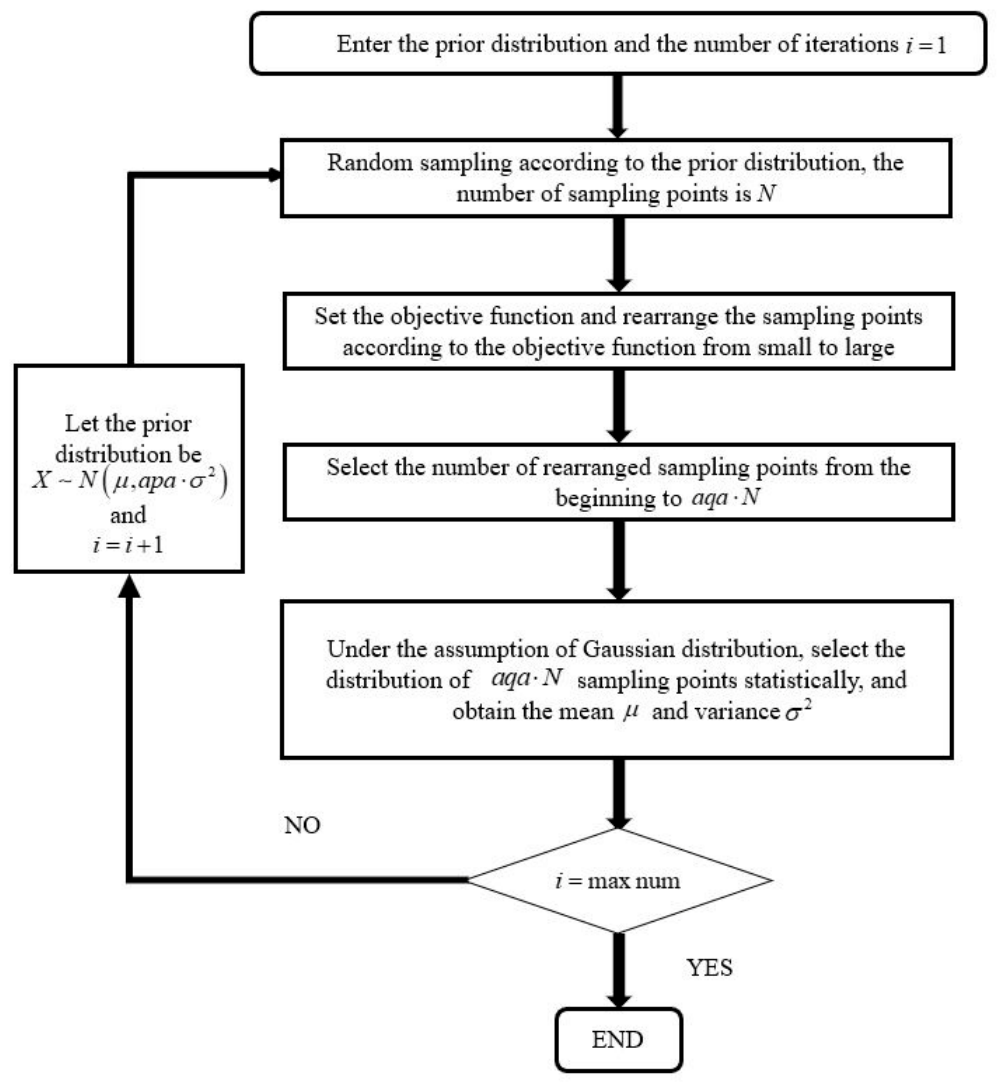
Figure 2.
Well A. (a) Density; (b) ; (c) ; (d) ; (e) P-wave velocity; (f) S-wave velocity; (g)Total porosity; (h) Clay content; (i) Water saturation.
Figure 2.
Well A. (a) Density; (b) ; (c) ; (d) ; (e) P-wave velocity; (f) S-wave velocity; (g)Total porosity; (h) Clay content; (i) Water saturation.
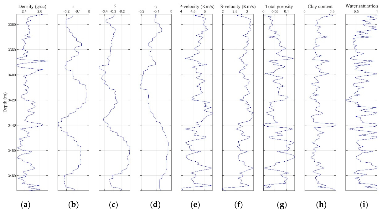
Figure 3.
Comparison between elastic parameters calculated from the corrected isotropic component of the rock-physical model and logging elastic parameters (a) Density; (b) P-wave velocity; (c) S-wave velocity.
Figure 3.
Comparison between elastic parameters calculated from the corrected isotropic component of the rock-physical model and logging elastic parameters (a) Density; (b) P-wave velocity; (c) S-wave velocity.
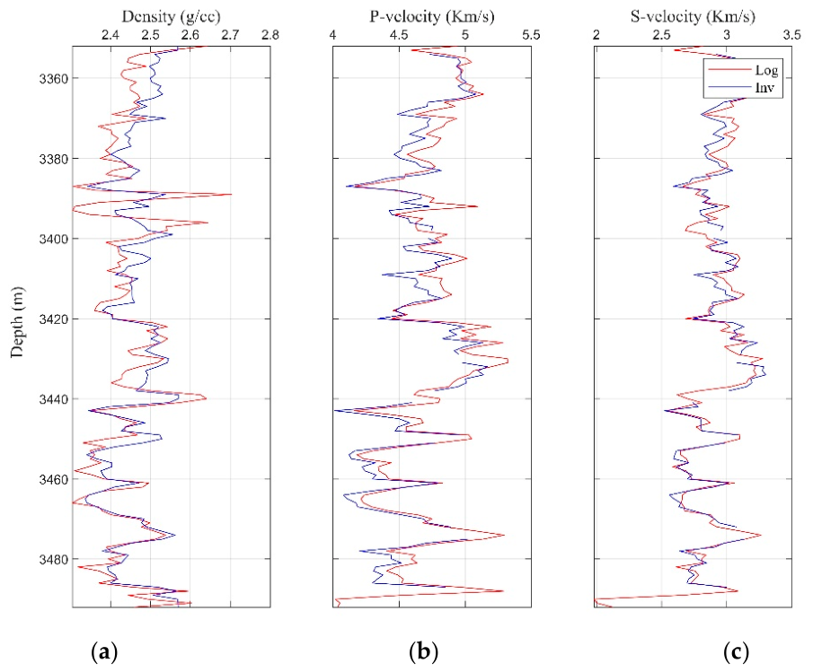
Figure 4.
Error and absolute error distribution between P- and S-wave velocities calculated by the rock physics model corrected with inverted mineral elastic moduli and logging-measured.
Figure 4.
Error and absolute error distribution between P- and S-wave velocities calculated by the rock physics model corrected with inverted mineral elastic moduli and logging-measured.
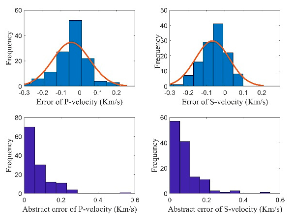
Figure 5.
Physical parameter inversion results of Well A. (a) pore porosity; (b) oriented fracture porosity; (c) azimuth of oriented fractures; (d) pore aspect ratio; € clay content; (f)Total porosity.
Figure 5.
Physical parameter inversion results of Well A. (a) pore porosity; (b) oriented fracture porosity; (c) azimuth of oriented fractures; (d) pore aspect ratio; € clay content; (f)Total porosity.
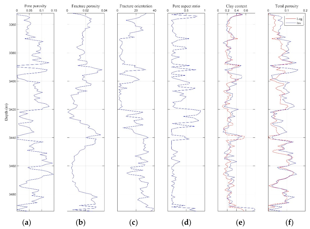
Figure 6.
Comparison of P-wave velocity, S-wave velocity and anisotropic parameters calculated from the physical parameters in Figure 5 with logging curves. (a) ; (b) ; (c) ; (d) P-wave velocity; € S-wave velocity.
Figure 6.
Comparison of P-wave velocity, S-wave velocity and anisotropic parameters calculated from the physical parameters in Figure 5 with logging curves. (a) ; (b) ; (c) ; (d) P-wave velocity; € S-wave velocity.
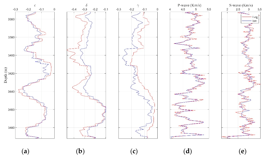
Figure 7.
Reflection coefficients vary with azimuth angles and incident angles.: (a) Reflection coefficients at different azimuth angles with a fixed incident angle ; (b) Reflection coefficients at incident angles with a fixed different azimuth angle .
Figure 7.
Reflection coefficients vary with azimuth angles and incident angles.: (a) Reflection coefficients at different azimuth angles with a fixed incident angle ; (b) Reflection coefficients at incident angles with a fixed different azimuth angle .
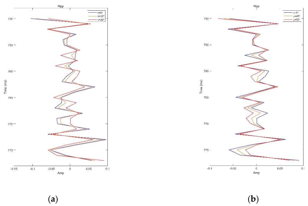
Figure 8.
Synthetic seismic records with different azimuth angles and incident angles using wavelets with dominant frequencies of 160 Hz and 40 Hz respectively: (a) Variations of incident angles at an azimuth angle of 0° with a dominant wavelet frequency of 160 Hz; (b) Variations of incident angles at an azimuth angle of 45° with a dominant wavelet frequency of 160 Hz; (c) Variations of incident angles at an azimuth angle of 90° with a dominant wavelet frequency of 160 Hz; (d) Variations of incident angles at an azimuth angle of 0° with a dominant wavelet frequency of 40 Hz; € Variations of incident angles at an azimuth angle of 45° with a dominant wavelet frequency of 40 Hz; (f) Variations of incident angles at an azimuth angle of 90° with a dominant wavelet fre-quency of 40 Hz.
Figure 8.
Synthetic seismic records with different azimuth angles and incident angles using wavelets with dominant frequencies of 160 Hz and 40 Hz respectively: (a) Variations of incident angles at an azimuth angle of 0° with a dominant wavelet frequency of 160 Hz; (b) Variations of incident angles at an azimuth angle of 45° with a dominant wavelet frequency of 160 Hz; (c) Variations of incident angles at an azimuth angle of 90° with a dominant wavelet frequency of 160 Hz; (d) Variations of incident angles at an azimuth angle of 0° with a dominant wavelet frequency of 40 Hz; € Variations of incident angles at an azimuth angle of 45° with a dominant wavelet frequency of 40 Hz; (f) Variations of incident angles at an azimuth angle of 90° with a dominant wavelet fre-quency of 40 Hz.
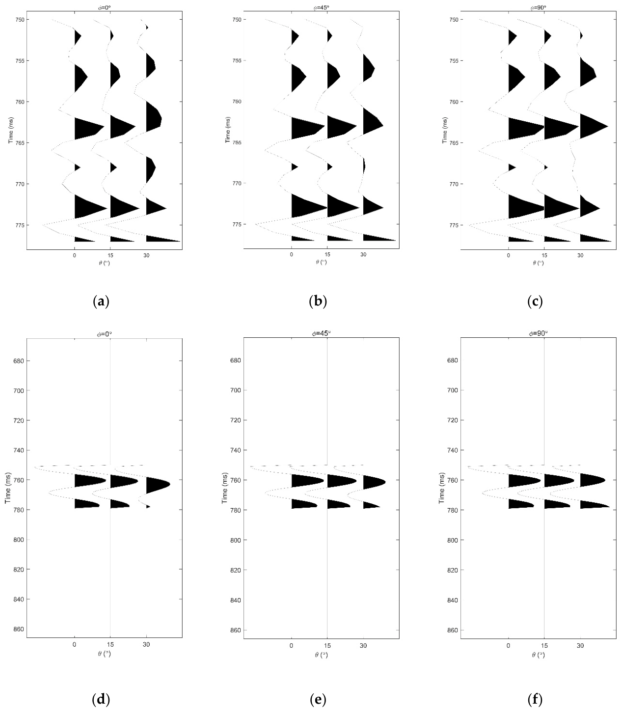
Figure 9.
Influence of pore porosity variation on synthetic seismic records at different incident angles using wavelets with dominant frequencies of 160 Hz and 40 Hz respectively: (a) 160 Hz dominant wavelet frequency, logging total porosity; (b) 160 Hz dominant wavelet frequency, pore porosity of 0.2; (c) 160 Hz dominant wavelet frequency, pore porosity of 0.3; (d) 40 Hz dominant wavelet frequency, logging total porosity; I 40 Hz dominant wavelet frequency, pore porosity of 0.2; (f) 40 Hz dominant wavelet frequency, pore porosity of 0.3.
Figure 9.
Influence of pore porosity variation on synthetic seismic records at different incident angles using wavelets with dominant frequencies of 160 Hz and 40 Hz respectively: (a) 160 Hz dominant wavelet frequency, logging total porosity; (b) 160 Hz dominant wavelet frequency, pore porosity of 0.2; (c) 160 Hz dominant wavelet frequency, pore porosity of 0.3; (d) 40 Hz dominant wavelet frequency, logging total porosity; I 40 Hz dominant wavelet frequency, pore porosity of 0.2; (f) 40 Hz dominant wavelet frequency, pore porosity of 0.3.
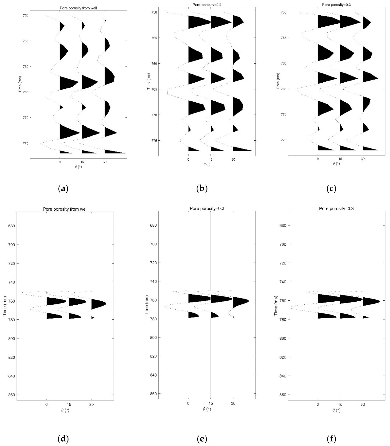
Figure 10.
Influence of azimuth variation of oriented fractures on synthetic seismic records at different observation azimuths using wavelets with dominant frequency of 40 Hz: (a) Predicted fracture azimuth based on logging data of Well A; (b) Oriented fracture azimuth of 0°; (c) Oriented fracture azimuth of 45°; (d) Oriented fracture azimuth of 90°.
Figure 10.
Influence of azimuth variation of oriented fractures on synthetic seismic records at different observation azimuths using wavelets with dominant frequency of 40 Hz: (a) Predicted fracture azimuth based on logging data of Well A; (b) Oriented fracture azimuth of 0°; (c) Oriented fracture azimuth of 45°; (d) Oriented fracture azimuth of 90°.
Disclaimer/Publisher’s Note: The statements, opinions and data contained in all publications are solely those of the individual author(s) and contributor(s) and not of MDPI and/or the editor(s). MDPI and/or the editor(s) disclaim responsibility for any injury to people or property resulting from any ideas, methods, instructions or products referred to in the content. |
© 2026 by the authors. Licensee MDPI, Basel, Switzerland. This article is an open access article distributed under the terms and conditions of the Creative Commons Attribution (CC BY) license.
Copyright: This open access article is published under a Creative Commons CC BY 4.0 license, which permit the free download, distribution, and reuse, provided that the author and preprint are cited in any reuse.


