

Submitted:
06 July 2026
Posted:
07 July 2026
You are already at the latest version
Abstract
Always-on keyword spotting (KWS) on microcontrollers must reconcile high recognition accuracy with severe constraints on memory, computation, and energy. Most small-footprint KWS research targets English, and its conclusions remain largely unverified for typologically different, consonant-rich languages such as Polish. In this work, we present a complete, hardware-validated KWS solution for Polish on the RP2350 microcontroller (Raspberry Pi Pico 2). We design three compact architectures from the convolutional (CNN), convolutional-recurrent (CRNN), and depthwise-separable (DS-CNN) families and benchmark them against BC-ResNet, a state-of-the-art reference, on a 25-keyword Polish vocabulary using MFCC features. All models are evaluated in full precision (Float32) and after 8-bit integer (INT8) post-training quantization, with inference latency measured directly on the target hardware. BC-ResNet attains the highest full-precision accuracy (97.81%) but is the most fragile under quantization, whereas the proposed CRNN becomes the most accurate quantized model (94.28%), the DS-CNN the smallest (46.15 KB), and the CNN the fastest (107.5 ms); all quantized models meet a one-second real-time budget. We further show that the accuracy ranking inverts after quantization, that memory savings are highly architecture-dependent, and that phonetically similar Polish words are the dominant source of error. These results offer practical guidance for deploying small-footprint KWS in Polish and other under-represented languages.
Keywords:
keyword spotting
; small-footprint speech recognition
; Polish language
; TinyML
; microcontroller
; RP2350
; Raspberry Pi Pico 2
; INT8 quantization
; depthwise separable convolution
; CRNN
; MFCC
1. Introduction
Voice interfaces have become one of the most natural and ergonomic methods of human–machine interaction. Keyword Spotting (KWS) is the task of detecting predefined words or short phrases in a continuous audio stream. It constitutes the foundation of modern virtual assistants, such as Amazon Alexa, Apple Siri, and Google Assistant, where a lightweight, always-on detector listens for a wake word before activating more complex processing pipelines.
With the rapid expansion of the Internet of Things (IoT), there is a growing demand for touchless operation of smart-home appliances and industrial automation systems. However, streaming audio to remote cloud servers introduces critical challenges, including unacceptable latency, high network bandwidth usage, increased power consumption, and privacy concerns regarding user data [1]. A remedy is offered by Edge Computing and the TinyML paradigm, which shift acoustic analysis directly onto low-cost microcontrollers at the edge of the network.
Historically, speech recognition was dominated by Hidden Markov Models (HMMs) combined with Gaussian Mixture Models (GMMs), which successfully captured the sequential and stochastic nature of speech [2]. For microcontrollers operating in an always-on listening mode with only hundreds of kilobytes of RAM, however, these classical models proved too resource-hungry and energy-inefficient [3].
These limitations were largely overcome by deep learning, which replaced HMM decoding with neural networks that predict keyword probabilities directly from acoustic features, such as Mel-Frequency Cepstral Coefficients (MFCCs) [3]. Over the past decade, a range of specialized small-footprint architecture families has emerged—convolutional (CNN), convolutional-recurrent (CRNN), depthwise-separable (DS-CNN), and broadcasted-residual (BC-ResNet) networks—which are reviewed in detail in Section 2.
The overwhelming majority of small-footprint KWS studies have been developed and evaluated on English data, most notably on the Google Speech Commands dataset [4], and the transferability of their conclusions to typologically different languages remains largely unverified. Here, we target Polish, a West Slavic language spoken by approximately 40 million people, whose phonological profile differs considerably from that of English. Polish is characterized by a consonant-rich phonology with long and dense consonant clusters (e.g., the keyword wstecz, “backward”, begins with a three-consonant cluster) and an unusually large inventory of fricatives and affricates, including a typologically rare three-way place contrast between dental, retroflex, and alveolo-palatal sibilants [5]. In addition, its rich inflectional morphology gives rise to numerous phonetically similar word forms. These properties make Polish keywords particularly difficult to discriminate when the effective spectral resolution is reduced—as exemplified in our experiments by near-minimal pairs such as ptak (“bird”) and tak (“yes”)—and thus make Polish a demanding and informative test case for resource-constrained KWS.
In this work, we present a complete, hardware-validated KWS solution for the Polish language targeting devices with severely constrained resources. Throughout the paper, we distinguish between an architecture family (a general class of network designs established in the literature, e.g., CRNN), an architecture (a concrete instantiation of a family, i.e., a specific configuration of layers, their dimensions, and the resulting parameter count), and a model (a trained instance of an architecture). The main contributions of this paper are as follows:
- We design three original, compact architectures—belonging to the CNN, CRNN, and DS-CNN families—tailored to Polish-language KWS on microcontrollers, and we benchmark them against BC-ResNet [6], a state-of-the-art reference architecture for small-footprint KWS.
- We provide a systematic evaluation of small-footprint KWS for the Polish language, which remains under-represented in the KWS literature dominated by English-language benchmarks. All models are trained and evaluated on a dataset of 25 Polish keywords.
- We study the effect of post-training 8-bit integer (INT8) quantization, a crucial step for TinyML deployments [1,7], on accuracy, model size, and inference latency. Notably, we show that the accuracy ranking of the evaluated architectures inverts after quantization, and that the most parameter-efficient architecture does not necessarily yield the fastest or most robust quantized model.
- We deploy and benchmark the complete system on custom-designed hardware: a dedicated printed circuit board (PCB) integrating the Raspberry Pi Pico 2 board with the RP2350 microcontroller and an analog audio front-end based on an electret microphone, on which all inference latencies are measured.
The remainder of this paper is organized as follows. Section 2 reviews related work on small-footprint KWS. Section 3 introduces the necessary background: the KWS problem, MFCC feature extraction, TinyML, model quantization, and inference frameworks for microcontrollers. Section 4 describes the proposed network architectures. Section 5 presents the hardware platform and the experimental results, and Section 6 discusses the findings. Finally, Section 7 concludes the paper.
2. Related Works
Early speech recognition systems employed statistical sequence modelling, which led to the long-standing dominance of Hidden Markov Models (HMMs). HMMs successfully captured the sequential and stochastic nature of speech [2]. In HMM-based KWS systems, a keyword model is compared against a background noise or filler model, and the Viterbi search algorithm is used to find the optimal path through the decoding graph. However, deploying HMM-based models on microcontrollers is demanding, as Viterbi decoding requires considerable computational and memory resources [1].
In 2014, Chen et al. demonstrated that Deep Neural Networks (DNNs) can effectively replace HMMs for small-footprint KWS [8]. Their system predicts keyword probabilities directly from acoustic features, eliminating the need for complex sequence search algorithms such as Viterbi decoding. This reduced latency and simplified the computational requirements, making the approach attractive for real-time applications. The main drawback of plain DNNs, however, is their inability to exploit the local temporal and spectral correlations present in the speech signal.
To overcome this limitation, Sainath and Parada introduced Convolutional Neural Networks (CNNs) to the KWS domain [9]. By treating the extracted acoustic features as two-dimensional images, CNNs effectively capture local time–frequency patterns and achieve higher accuracy with fewer parameters than DNNs.
Arik et al. proposed the Convolutional Recurrent Neural Network (CRNN) for KWS [10], in which convolutional layers first extract local features and recurrent layers subsequently encode the global temporal context. This combination achieves high accuracy and noise robustness with a relatively small memory footprint [1].
A further step towards efficiency was the Depthwise Separable Convolutional Neural Network (DS-CNN), inspired by the MobileNet architecture [11]. Zhang et al., in their “Hello Edge” study [3], demonstrated that factorising standard convolutions into separate depthwise and pointwise (1×1) operations drastically reduces the parameter count and computational load. Their DS-CNN model achieved an accuracy of 95.4% on the Google Speech Commands dataset [3,4].
More recently, Kim et al. introduced broadcasted residual learning and the BC-ResNet architecture to address the computational trade-off between 1D and 2D convolutions [6]. Standard 1D temporal convolutions are efficient but lack invariance along the frequency dimension, whereas 2D convolutions are computationally demanding. BC-ResNet resolves this by performing frequency-wise convolutions on 2D features, averaging them into 1D temporal features, and then broadcasting the 1D residual information back onto the 2D spatial dimensions. The BC-ResNet-1 model achieved state-of-the-art performance (96.6% accuracy) with fewer than 10k parameters on the Google Speech Commands dataset [1,6].
Notably, all of the above milestones were established on English data, with the Google Speech Commands dataset [4] serving as the de facto standard benchmark. Research on KWS for other languages has gained momentum only recently. Mazumder et al. released the Multilingual Spoken Words Corpus, covering more than 340,000 keywords in 50 languages [12], and proposed a few-shot transfer-learning approach that enables keyword spotting in a new language from only a handful of training examples [13]. Multilingual speech-command collections derived from crowd-sourced recordings, such as the 15-language dataset used in this work [14], follow the same direction. Nevertheless, Slavic languages—including Polish, whose consonant-rich phonology and dense consonant clusters [5] pose specific challenges for acoustic modelling—remain scarcely represented in the small-footprint KWS literature. To the best of our knowledge, no prior work has systematically benchmarked small-footprint KWS architectures for Polish, covering both full-precision and quantized models together with latency measurements on physical microcontroller hardware. The present study addresses this gap.
3. Preliminaries
3.1. Keyword Spotting Problem
The workflow of a deep learning-based KWS system involves three main stages: extraction of acoustic features from the raw speech signal, application of a deep neural network model that generates probabilities for the individual keywords, and a decision stage that detects the presence of the target keywords [1].
KWS is a dynamic process in which the system continuously monitors the input audio signal and produces a sequence of posterior probabilities in real time. The feature extraction function converts the raw signal into a concise spectral representation: a two-dimensional matrix containing a temporal series of K-dimensional feature vectors, of which the model sequentially processes overlapping segments [1].
The deep learning model maps each temporal input segment to an N-dimensional vector representing the probability distribution over N keyword classes. The system then selects the class with the highest probability; if the score of the targeted keyword class exceeds a preset threshold, the keyword is detected, otherwise the segment is rejected as background noise or an unknown word [1].
3.2. Feature Extraction
Raw audio waveforms must first be transformed into a compact and reliable representation. The most widely adopted feature extraction method in speech processing is Mel-Frequency Cepstral Coefficients (MFCCs). These acoustic features mimic human sound perception by reflecting the nonlinear frequency sensitivity of the human ear [15,16].
The standard feature extraction pipeline is shown in Figure 1. It consists of several sequential digital signal processing blocks: pre-emphasis, framing, windowing, the Fast Fourier Transform (FFT), the application of a Mel filter bank, logarithmic compression, and the Discrete Cosine Transform (DCT) [15,16].
Figure 2 illustrates the successive representations of a one-second speech-like signal: the raw waveform, its log-Mel spectrogram, and the resulting MFCC matrix. The final representation is a compact two-dimensional image whose horizontal axis corresponds to time and whose vertical axis corresponds to the cepstral coefficients.
First, a pre-emphasis filter is applied to the raw audio signal to boost its high-frequency components, since speech energy is concentrated in the low-frequency band; this balances the spectrum and increases the amount of information available to the model. Next, the signal is segmented into overlapping frames (typically 30–40 ms long with a 25–75% shift), which captures the quasi-stationary nature of speech. Each frame is then multiplied by a window function (most commonly a Hamming window) to reduce spectral leakage, and the FFT is applied to compute the power spectrum. The spectrum is subsequently passed through a bank of triangular band-pass filters spaced according to the Mel scale, and a logarithm is applied to the filter bank outputs to imitate the loudness perception of the human ear. Finally, the DCT is applied to decorrelate the log-energies and reduce their dimensionality, yielding the MFCC matrix. The resulting features are treated as two-dimensional images and used as the input to the neural networks [15].
3.3. TinyML and Model Quantization
Tiny Machine Learning (TinyML) is a subfield of artificial intelligence and edge computing that focuses on deploying machine learning and deep learning models directly on ultra-low-power, resource-constrained embedded devices, especially microcontrollers. Such platforms often feature less than 500 KB of SRAM, less than 2 MB of Flash storage, and severe energy constraints [17].
To fit deep neural networks into microcontrollers, neural network quantization is commonly applied as an optimization step. Quantization reduces the numerical precision of the network weights and intermediate activation maps: during the conversion of a trained model, 32-bit floating-point values are mapped to lower-precision formats, such as signed 8-bit integers. This conversion shrinks the model size and removes the dependence on a Floating-Point Unit (FPU), drastically reducing inference latency and energy consumption [7].
3.4. Inference Frameworks
The deployment of models on edge hardware relies on specialized software frameworks. Several libraries are available for running neural network models on microcontrollers. In this work, we use TensorFlow Lite for Microcontrollers (TFLM, now part of LiteRT), an open-source library developed by Google as a reduced version of TensorFlow Lite [18]. It does not require an underlying operating system and is designed specifically for model inference on microcontrollers and other edge devices.
To execute a model, a FlatBuffer is created from the .tflite file and loaded into an interpreter, together with a pre-allocated tensor arena (a static memory buffer used for the input, output, and working tensors during inference). TFLM relies heavily on optimized backend libraries, such as the Cortex Microcontroller Software Interface Standard Neural Network (CMSIS-NN) library provided by ARM [19,20], which offers highly optimized implementations of neural network kernels for ARM Cortex-M processors.
4. Implementation
4.1. Neural Network Architectures
Three original, compact architectures were designed, trained, and evaluated: a CNN, belonging to the family introduced by Sainath and Parada [9]; a CRNN, following the design of Arik et al. [10]; and a DS-CNN inspired by the architecture proposed in [3]. In addition, the BC-ResNet architecture [6] was reimplemented as a state-of-the-art reference for benchmarking. All models were engineered to process two-dimensional MFCC features as input. Each architecture was kept within a small-footprint budget suitable for microcontroller deployment, ranging from approximately 13k parameters for the BC-ResNet reference to 76k for the CNN (Table 1). As discussed in Section 5, parameter count alone is not predictive of accuracy in this regime: the largest model (CNN) is in fact the least accurate, indicating that the inductive bias of each architecture family, rather than raw capacity, is the dominant factor.
The CNN model is designed to function as an acoustic feature extractor. The model architecture is shown in Figure 3. The architecture utilizes standard two-dimensional convolutional layers to capture local time-frequency correlations, such as formants and pitch shifts. The multidimensional output is subsequently flattened and processed through fully connected dense layers, culminating in a Softmax classifier that outputs the target vocabulary probabilities.
To better capture the sequential nature of speech, a hybrid CRNN architecture was implemented (Figure 4). The initial convolutional layer forms a spatial front-end that reduces the input dimensionality. Next, the spatial dimensions are flattened while the temporal axis is preserved, forming a time-series representation. This is fed into a single GRU layer with 32 units (see Figure 4), which allows the model to capture long-term phonetic dependencies. The final layer is a dense classification layer with a Softmax activation.
The DS-CNN architecture design is based on [3]. Model structure is shown in the Figure 6. The model contains 4 DS blocks (Figure 5). Each block consists of a Depthwise Phase and a Pointwise Phase. In the Depthwise part, a spatial filtering step applies a kernel independently to each input channel. It is followed by Batch Normalization for training stabilization and a ReLU activation function. In the Pointwise part, a convolution is used to linearly combine the feature maps generated by the depthwise phase into output channels. As in the first phase, it is followed by Batch Normalization and a ReLU activation function.
The CNN, CRNN, and DS-CNN models were trained using the Adam optimizer with sparse categorical cross-entropy loss over a maximum of 20 epochs, with a batch size of 64 or 128 (model-dependent) and early stopping (patience = 3, restoring best weights). The BC-ResNet model followed the training recipe from the original paper [6]: SGD optimizer with momentum 0.9, L2 weight decay 0.001, an initial learning rate of 0.1 with a 2-epoch warmup and cosine/stepwise decay, over 20 epochs with a batch size of 128.
The dataset was partitioned into a training subset (80%, 112,677 samples) and a test subset (20%, 28,169 samples) using a fixed random seed. The split was not explicitly speaker-independent. Five-fold cross-validation was applied on the training subset for model selection; final accuracy was evaluated on the shared test set.
Regularization was applied in the form of early stopping on validation loss (CNN, CRNN, DS-CNN) and L2 weight decay (BC-ResNet). Data augmentation in the form of white noise injection was applied to the training set only; additional augmentations (pitch shifting, time stretching, and noise) were provided by the dataset authors. All training was performed in TensorFlow/Keras (CNN, CRNN, DS-CNN) and PyTorch (BC-ResNet) on a single NVIDIA GeForce GTX 1050 Ti GPU.
The total number of parameters for each architecture is summarized in Table 1.
5. Results
5.1. Hardware Architecture
In order to investigate the performance of the proposed neural networks in a real-world scenario, a dedicated hardware platform was developed. The system architecture revolves around the Raspberry Pi Pico 2 development board, which features the RP2350 microcontroller (Figure 7). The RP2350 is a high-performance system-on-chip (SoC) that employs a unique dual-core, dual-architecture design, providing two Arm Cortex-M33 cores and two RISC-V Hazard3 cores, both operating at a nominal frequency of 150 MHz [21].
In this research, the Arm Cortex-M33 cores were selected due to support for TinyML workloads, such as CMSIS-DSP [22] and Tensorflow Lite for Microcontrollers [18]. The Cortex-M33 implements the Armv8-M architecture, which includes Digital Signal Processing (DSP) instructions and a Single-Precision Floating-Point Unit (FPU). These hardware features are critical for efficient Keyword Spotting (KWS), as they allow for the accelerated computation of Mel-Frequency Cepstral Coefficients (MFCC) and optimize the execution of quantized neural network kernels. The microcontroller is equipped with 520 KB of on-chip SRAM. The Pico 2 board also provides 4 MB of external QSPI Flash memory [21].
The hardware implementation includes a custom dual-layer Printed Circuit Board (PCB) designed and fabricated to interface the Raspberry Pi Pico 2 with an analog audio front-end. This front-end utilizes an electret microphone coupled with a low-noise pre-amplifier stage [23] to capture voice commands.
5.2. Testing on the Database
For testing the models, the dataset described in [14] was used. The database contains 1-second voice recordings of single words in 15 languages. All records have been augmented using time-shifting, noise injection, pitch variation, etc. [14]. For testing, only Polish words were selected. The models were trained to recognize 25 classes, which are shown in Table 2.
The overall performance and memory requirements of the evaluated neural network architectures were measured in their Float32 format and after integer quantization (INT8). Table 3 and Table 4 summarize the accuracy, F1-score, model size, and on-device inference time for the Float32 and INT8 variants, respectively. All reported F1-scores are weighted-averaged across classes (each class’s F1 weighted by its number of samples). Because the dataset is markedly imbalanced (e.g., no (nie) with 31,086 samples versus backward (wstecz) with 918), both the overall accuracy and the weighted F1-score are dominated by the most frequent classes; the per-class confusion-matrix analysis (Section 5, Confusion Matrix) is therefore included to give a more balanced view of per-keyword performance.
The highest accuracy in Float32 format was achieved by the BC-ResNet model (97.81%), followed closely by DS-CNN (97.06%) and CRNN (96.19%). The CNN architecture exhibited the lowest Float32 accuracy at 88.68%. After INT8 quantization, the CRNN model retained the highest accuracy (94.28%), while BC-ResNet experienced the largest absolute accuracy drop (5.08 percentage points). Quantization significantly reduced the model size for the CNN (from 300.64 KB to 79.44 KB) and DS-CNN (from 98.85 KB to 46.15 KB). The file sizes of the CRNN and BC-ResNet architectures remained largely unaffected by the quantization process. Inference time was measured directly on the target hardware platform, the Raspberry Pi Pico 2 microcontroller, as the mean over 100 consecutive inferences per model; all programs were compiled with Release optimization settings. The standard deviation did not exceed for any configuration and is therefore omitted. The resulting on-device latencies are reported alongside the accuracy and memory metrics in Table 3 and Table 4.
The shortest mean inference time was recorded for the CNN model in INT8 format ( ). The DS-CNN architecture exhibited the greatest relative speedup following INT8 quantization, with the mean inference time reduced from to (approximately 5.4-fold). In contrast, the BC-ResNet architecture showed the smallest relative improvement after quantization, with execution time decreasing from to . Relative to the one-second analysis window of the input frame, all INT8 models meet the real-time constraint, with inference well below 1 . In Float32, only the CNN and CRNN remain within this budget, whereas the DS-CNN ( ) exceeds it and is therefore unsuitable for continuous, always-on operation unless quantized.
5.3. Confusion Matrix
Confusion matrices were generated for all evaluated models to assess prediction stability across individual voice commands. In every matrix, rows correspond to the true class and columns to the predicted class, so a strong diagonal indicates correct predictions. The matrices for the BC-ResNet model, in both Float32 and INT8 formats, are shown in Figure 8; for conciseness, the corresponding matrices for the CNN, CRNN, and DS-CNN models are provided in Appendix A.
The BC-ResNet model demonstrated robust word recognition performance across the majority of classes in Float32 format. A notable exception was the keyword bird (ptak), which achieved 83.5% per-class accuracy and was most frequently misclassified as yes (tak) in 7.4% of cases and as two (dwa) in 4.9% of cases.
In the Float32 CNN model, the lowest classification accuracy was recorded for the command bird (ptak) at 70.8%, which was misclassified as yes (tak) in 16.9% of instances. A further notable error involved the keyword seven (siedem), which achieved only 72.7% accuracy and was most frequently confused with four (cztery) in 13.3% of cases.
The Float32 CRNN model exhibited generally strong per-class performance. The weakest classes were yes (tak) at 89.1%, one (jeden) at 91.7%, and go (iść) at 92.6%; the latter was occasionally misclassified as five (pięć) in 3.6% of cases.
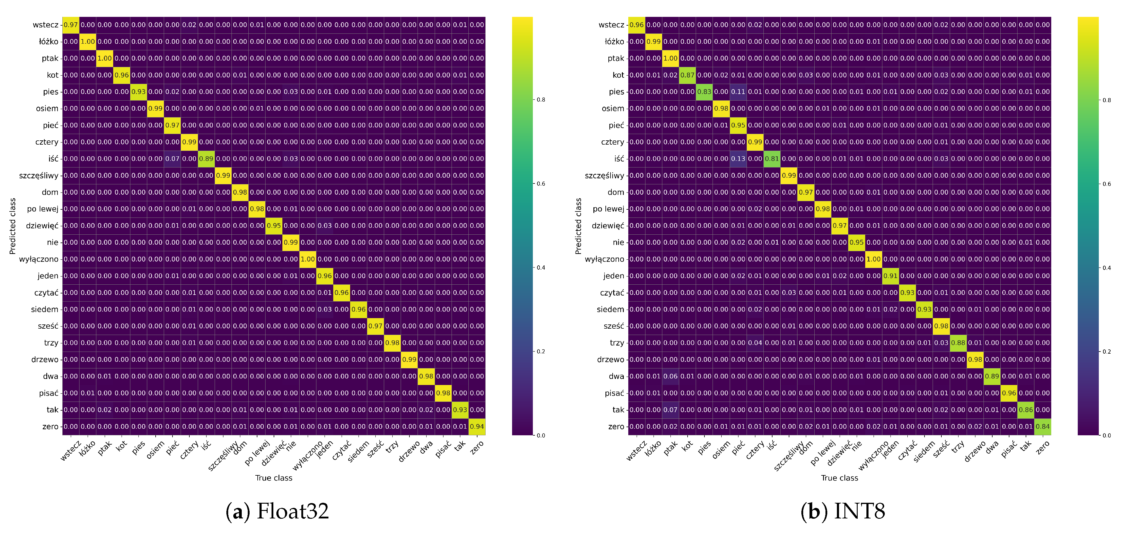
In the Float32 DS-CNN model, the weakest class was go (iść) at 88.8%, which was most frequently misclassified as five (pięć) in 6.7% of instances. The remaining classes maintained uniformly high per-class accuracy.
Following INT8 quantization, the BC-ResNet model exhibited a substantial accuracy degradation for the keyword bird (ptak), which fell to 39.9%. This word was most frequently recognized as yes (tak) (24.3%), two (dwa) (16.9%), and four (cztery) (7.4%), representing the most pronounced per-class degradation observed across all quantized models.
In the quantized CNN model, the keyword bird (ptak) dropped to 61.7%, with yes (tak) accounting for 21.0% of misclassifications. The class seven (siedem) also declined to 68.7% accuracy, primarily due to confusion with four (cztery) in 14.7% of cases.
For the quantized CRNN architecture, the majority of classes maintained satisfactory accuracy. The weakest classes were yes (tak) at 85.9%, seven (siedem) at 87.7% (confused with one (jeden) in 4.1% of cases), and go (iść) at 87.8% (confused with five (pięć) in 5.9% of cases).
In the quantized DS-CNN model, the weakest class was go (iść) at 80.9%, most frequently misclassified as five (pięć) in 13.4% of instances. The class dog (pies) also declined to 82.6% accuracy, with the primary source of confusion being five (pięć) in 10.6% of cases.
6. Discussion
Experimental results demonstrate that deploying high-accuracy Keyword Spotting (KWS) on a resource-constrained microcontroller like the RP2350 requires navigating various trade-offs. No single model excelled across all metrics, which included full-precision accuracy, robustness to INT8 quantization, memory footprint, and inference speed. Instead, each architecture offers distinct advantages, meaning the best choice depends heavily on the specific constraints of the target application.
In the full-precision (Float32) tests, the BC-ResNet model achieved the highest accuracy at 97.81% while remaining highly parameter-efficient, utilizing only 13,450 parameters. The DS-CNN and CRNN followed closely with scores of 97.06% and 96.19%, respectively. Conversely, the standard CNN lagged significantly at 88.68%, despite containing a massive 75,982 parameters. This confirms that architectures specifically designed for the time and frequency structures of speech—such as the specialized features in DS-CNN [3] and BC-ResNet—capture [6] audio patterns far more effectively than generic convolutional layers.
When INT8 quantization was applied to compress the models, the robustness rankings inverted. The CRNN proved most resilient, losing only 1.91 percentage points (96.19% → 94.28%), making it the most accurate quantized model. The DS-CNN experienced a moderate drop (97.06% → 93.13%). The BC-ResNet, however, suffered the most significant decrease, losing 5.08 percentage points (97.81% → 92.73%). This fragility was particularly noticeable with phonetically similar keywords; for instance, the Polish command ptak (bird) dropped to a 39.9% accuracy rate, frequently being confused with tak (yes) and dwa (two) (see Figure 8b). This sensitivity is likely due to BC-ResNet’s reliance on precise mathematical mappings for frequency analysis [6], where the reduced dynamic range of 8-bit arithmetic erodes critical spectral details. In contrast, the CRNN focuses more on temporal changes, making it more tolerant of minor rounding errors.
The impact of quantization on memory footprint also varied by architecture. The CNN and DS-CNN compressed significantly, shrinking down to 79.44 KB and 46.15 KB, respectively, making the DS-CNN the smallest deployed model in the study. The CRNN compressed only modestly by 16.5% to 182.62 KB, remaining the largest quantized model, as a significant portion of its footprint is attributed to metadata and structural elements rather than core weights. Strikingly, the BC-ResNet barely compressed at all, moving from 104.98 KB to just 101.97 KB. Because it already relies on very few parameters, its overall size is dominated by structural overhead rather than weight storage. Furthermore, the memory saved by compressing these few weights to 8 bits is almost entirely offset by the additional quantization metadata required by framework, such as scale and zero-point parameters for each tensor. This demonstrates that quantization does not uniformly result in a fourfold size reduction; the actual savings depend heavily on the model’s architectural design.
Inference latency, measured directly on the RP2350 (Table 3 and Table 4), revealed further differences. The DS-CNN experienced the most significant speed improvement from quantization, dropping from to (a 5.4× speedup). The standard CNN achieved the fastest quantized inference at ; however, given its lower accuracy of 85.32%, it is better suited as a low-power trigger than as a primary recognizer. The CRNN provided a strong balance, combining the highest quantized accuracy with a competitive latency. Conversely, the BC-ResNet gained minimal speed, shifting from to , only 1.15×. Despite having the lowest parameter count, its specific operations do not map efficiently to the integer kernels of the runtime system, making the most parameter-lean architecture paradoxically one of the slowest.
An analysis of classification errors across all architectures revealed a tendency to confuse words with similar phonetic structures. In the Polish dataset, ptak (bird) and tak (yes) share near-identical vocalic nucleus and coda, while iść (go) was frequently confused with pięć (five). Such pairs become increasingly difficult to distinguish as the effective spectral resolution is lowered by quantization. This pattern suggests that while Post-Training Quantization is sufficient for more robust architectures, Quantization-Aware Training [7] would likely be necessary for sensitive models like the BC-ResNet to preserve the subtle acoustic cues needed to separate these similar words.
The successful implementation on the custom PCB validated the RP2350 as a robust platform for TinyML. The ARM Cortex-M33 cores provided sufficient computational power, in particular by exploiting the DSP extension instructions of the Armv8-M architecture, which accelerate both the MFCC feature extraction (via the CMSIS-DSP library) and the quantized neural-network kernels (via the CMSIS-NN backend used by TensorFlow Lite for Microcontrollers). Future research could explore utilizing the dual-core capability of the RP2350 to pipeline the MFCC extraction and neural network inference stages, potentially decreasing latency further.
A key limitation of this study is that all reported metrics were obtained on the pre-recorded, augmented evaluation corpus rather than on live audio captured through the on-board acquisition chain. Consequently, the accuracy and F1-scores characterize the models together with the INT8 quantization and on-device latency behavior, but not the complete microphone-to-decision pipeline. Preliminary tests using live input from the electret-microphone front-end exhibited a marked degradation in recognition accuracy relative to the dataset evaluation. We attribute this gap primarily to a domain mismatch between the crowd-sourced training corpus and the audio captured by the custom front-end rather than to the network architectures themselves, which performed consistently on in-domain data. Acoustic analysis of the raw recordings (Table 5) substantiates this attribution along two independent dimensions: SNR estimated from the lowest-energy decile of frames (used as a noise-floor proxy in the absence of explicit silence segments) averaged (, range –), well below the threshold commonly required for reliable speech processing, and spectral analysis revealed a mean roll-off at (), far below the lower bound expected for narrowband-grade speech capture. RMS levels were consistent across recordings (range ) and no clipping was detected, ruling out gain misconfiguration or front-end saturation as contributing factors. Closing this gap will require characterizing and calibrating the analog front-end, collecting an in-domain dataset recorded directly through the target hardware, and applying domain-adaptation techniques together with quantization-aware training; we regard this microphone-level validation as essential future work before the prototype can serve as a consumer-grade voice interface.
7. Conclusions
This work presented a complete, hardware-validated keyword-spotting solution for the Polish language on a severely resource-constrained microcontroller. Three compact architectures from the CNN, CRNN, and DS-CNN families were designed and benchmarked against the state-of-the-art BC-ResNet reference, both in full precision and after INT8 quantization, with latency measured directly on the Raspberry Pi Pico 2 (RP2350).
The results show that no single architecture is optimal across all deployment criteria. BC-ResNet achieved the highest full-precision accuracy (97.81%) but proved the most fragile under quantization, whereas the proposed CRNN was the most robust and the most accurate quantized model (94.28%), the DS-CNN yielded the smallest INT8 footprint (46.15 KB), and the CNN delivered the lowest latency ( ). Notably, the accuracy ranking inverted after quantization, the memory savings were highly non-uniform across architectures, and all quantized models met the one-second real-time budget on the target device. Error analysis further revealed that the dominant failure mode is the confusion of phonetically similar Polish words (e.g., ptak/tak, iść/pięć), which is exacerbated by the reduced numerical precision of INT8 arithmetic.
These findings provide practical guidance for selecting and quantizing small-footprint KWS models for Polish and other consonant-rich, morphologically rich languages. The principal open challenge is bridging the gap between dataset-based evaluation and live microphone operation; addressing the acquisition-chain and domain-mismatch limitations discussed above, together with quantization-aware training, is the natural next step toward a deployable, always-on Polish voice interface.
Author Contributions
Conceptualization, J.S. and K.F.; methodology, J.S.; software, J.S.; validation, J.S.; formal analysis, J.S.; investigation, J.S.; resources, K.F.; data curation, J.S.; writing—original draft preparation, J.S.; writing—review and editing, J.S. and K.F.; visualization, J.S.; supervision, K.F.; project administration, K.F. All authors have read and agreed to the published version of the manuscript.
Funding
This research received no external funding.
Data Availability Statement
Conflicts of Interest
The authors declare no conflicts of interest.
Abbreviations
The following abbreviations are used in this manuscript:
| BC-ResNet | Broadcasted Residual Network |
| CMSIS | Cortex Microcontroller Software Interface Standard |
| CNN | Convolutional Neural Network |
| CRNN | Convolutional Recurrent Neural Network |
| DCT | Discrete Cosine Transform |
| DNN | Deep Neural Network |
| DS-CNN | Depthwise Separable Convolutional Neural Network |
| DSP | Digital Signal Processing |
| FFT | Fast Fourier Transform |
| FPU | Floating-Point Unit |
| GMM | Gaussian Mixture Model |
| GRU | Gated Recurrent Unit |
| HMM | Hidden Markov Model |
| INT8 | 8-bit Integer (precision) |
| IoT | Internet of Things |
| KWS | Keyword Spotting |
| MFCC | Mel-Frequency Cepstral Coefficients |
| PCB | Printed Circuit Board |
| QAT | Quantization-Aware Training |
| RMS | Root Mean Square |
| SGD | Stochastic Gradient Descent |
| SNR | Signal-to-Noise Ratio |
| SoC | System-on-Chip |
| SRAM | Static Random-Access Memory |
| TFLM | TensorFlow Lite for Microcontrollers |
| TinyML | Tiny Machine Learning |
Appendix A. Confusion Matrices for the CNN, CRNN, and DS-CNN Models
For completeness, this appendix reports the confusion matrices of the three proposed models in both Float32 and INT8 formats: the CNN (Figure A1), the CRNN (Figure A2), and the DS-CNN (Figure A3). The corresponding matrices for the BC-ResNet reference are given in the main text (Figure 8). In every matrix, rows correspond to the true class and columns to the predicted class, so a strong diagonal indicates correct predictions.
Figure A1.
Confusion matrices of the CNN model in (a) Float32 and (b) INT8 formats.
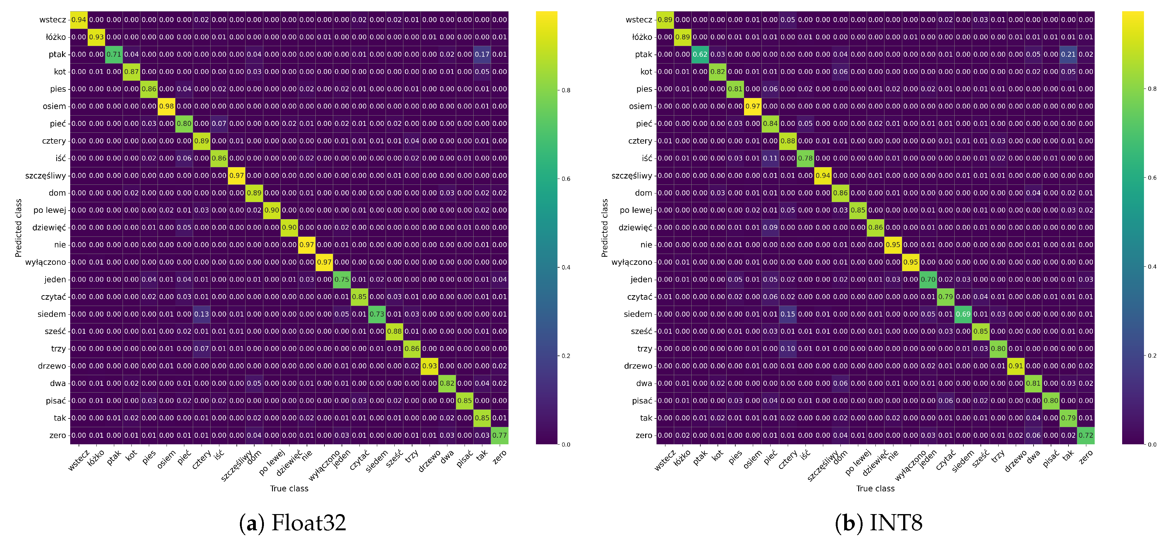
Figure A2.
Confusion matrices of the CRNN model in (a) Float32 and (b) INT8 formats.
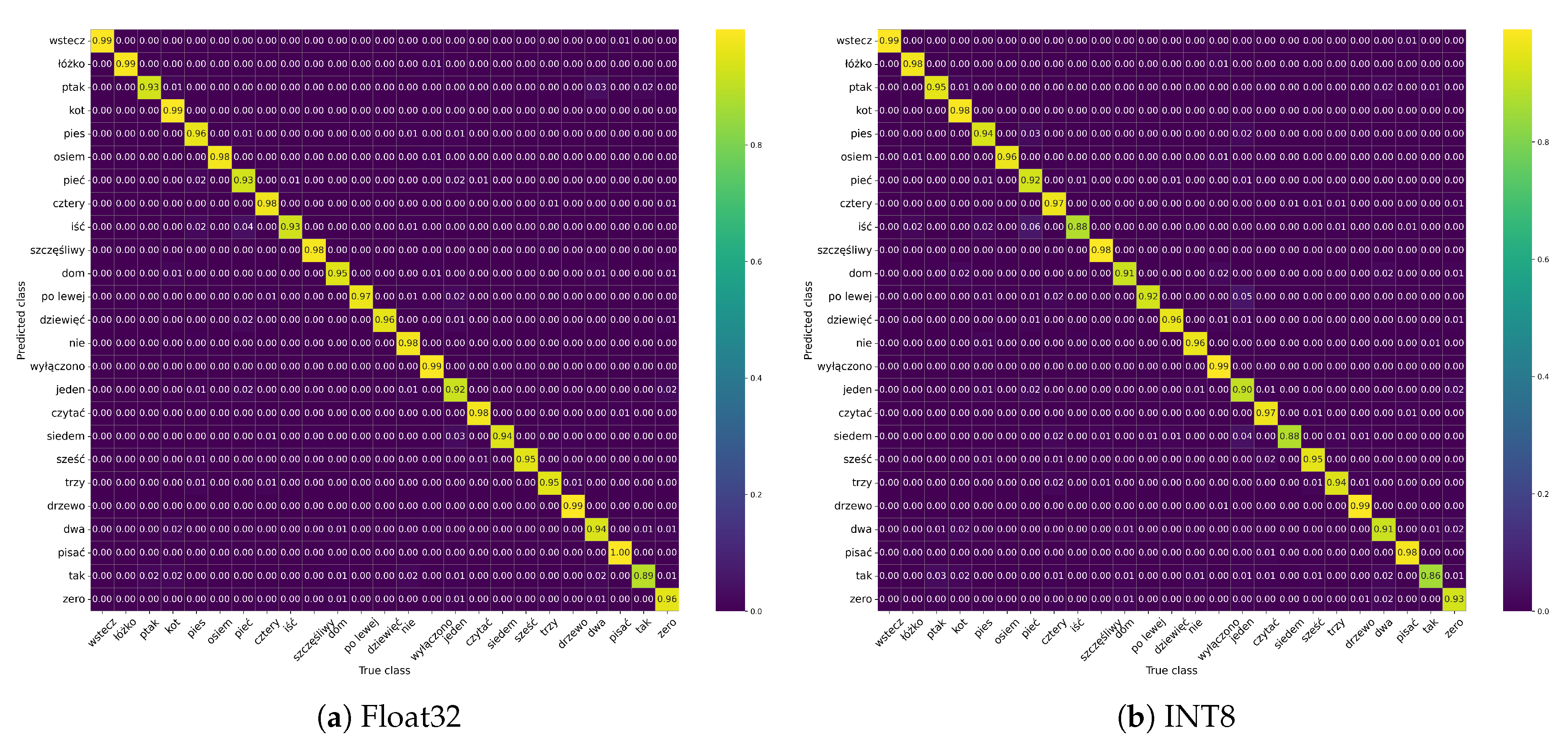
Figure A3.
Confusion matrices of the DS-CNN model in (a) Float32 and (b) INT8 formats.
References
- Garai, S.; Samui, S. Advances in Small-Footprint Keyword Spotting: A Comprehensive Review of Efficient Models and Algorithms. arXiv 2025, arXiv:eess. [Google Scholar]
- Rabiner, L. A tutorial on hidden Markov models and selected applications in speech recognition. Proc. IEEE 1989, 77, 257–286. [Google Scholar] [CrossRef] [PubMed]
- Zhang, Y.; Suda, N.; Lai, L.; Chandra, V. Hello Edge: Keyword Spotting on Microcontrollers. In arXiv; Arm, San Jose, CA: Stanford, CA; Stanford University, 2018. [Google Scholar]
- Warden, P. Speech Commands: A Dataset for Limited-Vocabulary Speech Recognition. arXiv 2018, arXiv:cs. [Google Scholar]
- Jassem, W. Polish. J. Int. Phon. Assoc. 2003, 33, 103–107. [Google Scholar] [CrossRef]
- Kim, B.; Chang, S.; Lee, J.; Sung, D. Broadcasted Residual Learning for Efficient Keyword Spotting. arXiv 2023, arXiv:cs. [Google Scholar]
- Jacob, B.; Kligys, S.; Chen, B.; Zhu, M.; Tang, M.; Howard, A.; Adam, H.; Kalenichenko, D. Quantization and Training of Neural Networks for Efficient Integer-Arithmetic-Only Inference. arXiv 2017, arXiv:cs. [Google Scholar]
- Chen, G.; Parada, C.; Heigold, G. Small-footprint keyword spotting using deep neural networks. In Proceedings of the 2014 IEEE International Conference on Acoustics, Speech and Signal Processing (ICASSP), 2014; pp. 4087–4091. [Google Scholar] [CrossRef]
- Sainath, T.N.; Parada, C. Convolutional neural networks for small-footprint keyword spotting. Proc. Interspeech 2015, 2015, 1478–1482. [Google Scholar] [CrossRef]
- Arik, S.O.; Kliegl, M.; Child, R.; Hestness, J.; Gibiansky, A.; Fougner, C.; Prenger, R.; Coates, A. Convolutional recurrent neural networks for small-footprint keyword spotting. arXiv 2017, arXiv:1703.05390. [Google Scholar]
- Howard, A.G.; Zhu, M.; Chen, B.; Kalenichenko, D.; Wang, W.; Weyand, T.; Andreetto, M.; Adam, H. MobileNets: Efficient Convolutional Neural Networks for Mobile Vision Applications. arXiv 2017, arXiv:cs. [Google Scholar]
- Mazumder, M.; Chitlangia, S.; Banbury, C.; Kang, Y.; Ciro, J.M.; Achorn, K.; Galvez, D.; Sabini, M.; Mattson, P.; Kanter, D.; et al. Multilingual Spoken Words Corpus. In Proceedings of the Proceedings of the NeurIPS Track on Datasets and Benchmarks, 2021. [Google Scholar]
- Mazumder, M.; Banbury, C.; Meyer, J.; Warden, P.; Reddi, V.J. Few-Shot Keyword Spotting in Any Language. Proc. Proc. Interspeech 2021, 2021, 4214–4218. [Google Scholar] [CrossRef]
- Muratov, A. multilingual-speech-commands-15lang-zip [Dataset]. 2025. Available online: https://huggingface.co/datasets/artur-muratov/multilingual-speech-commands-15lang-zip (accessed on 10 marzec 2026).
- Abdulsatar, A.A.; Davydov, V.V.; Yushkova, V.V.; Glinushkin, A.P.; Rud, V.Y. Age and gender recognition from speech signals. J. Phys. Conf. Ser. 2019, 1410, 012073. [Google Scholar] [CrossRef]
- Davis, S.; Mermelstein, P. Comparison of parametric representations for monosyllabic word recognition in continuously spoken sentences. IEEE Trans. Acoust. Speech Signal Process. 1980, 28, 357–366. [Google Scholar] [CrossRef]
- Ray, P.P. A review on TinyML: State-of-the-art and prospects. J. King Saud. Univ.-Comput. Inf. Sci. 2022, 34, 1595–1623. [Google Scholar] [CrossRef]
- Developers, TensorFlow. TensorFlow Lite for Microcontrollers, 2026. Dostęp. 2026.
- Lai, L.; Suda, N.; Chandra, V. CMSIS-NN: Efficient Neural Network Kernels for Arm Cortex-M CPUs, 2018. arXiv arXiv:cs.
- David, R.; Duke, J.; Jain, A.; Reddi, V.J.; Jeffries, N.; Li, J.; Kreeger, N.; Nappier, I.; Natraj, M.; Regev, S.; et al. TensorFlow Lite Micro: Embedded Machine Learning on TinyML Systems. arXiv 2021, arXiv:cs. [Google Scholar]
- Raspberry Pi Ltd. Raspberry Pi Pico 2 Datasheet An RP2350-based microcontroller board; Raspberry Pi Ltd, 2024. [Google Scholar]
- Arm Limited. CMSIS-DSP Documentation Version CMSIS 6; Accessed; Arm Limited, 2026; (accessed on 2026-01-29). [Google Scholar]
- Caldwell, J. Single-Supply, Electret Microphone Pre-Amplifier Reference Design. In TI Designs - Precision: Verified Design TIDU765; Texas Instruments, 2015. [Google Scholar]
Figure 1.
Block diagram of the MFCC extraction process.
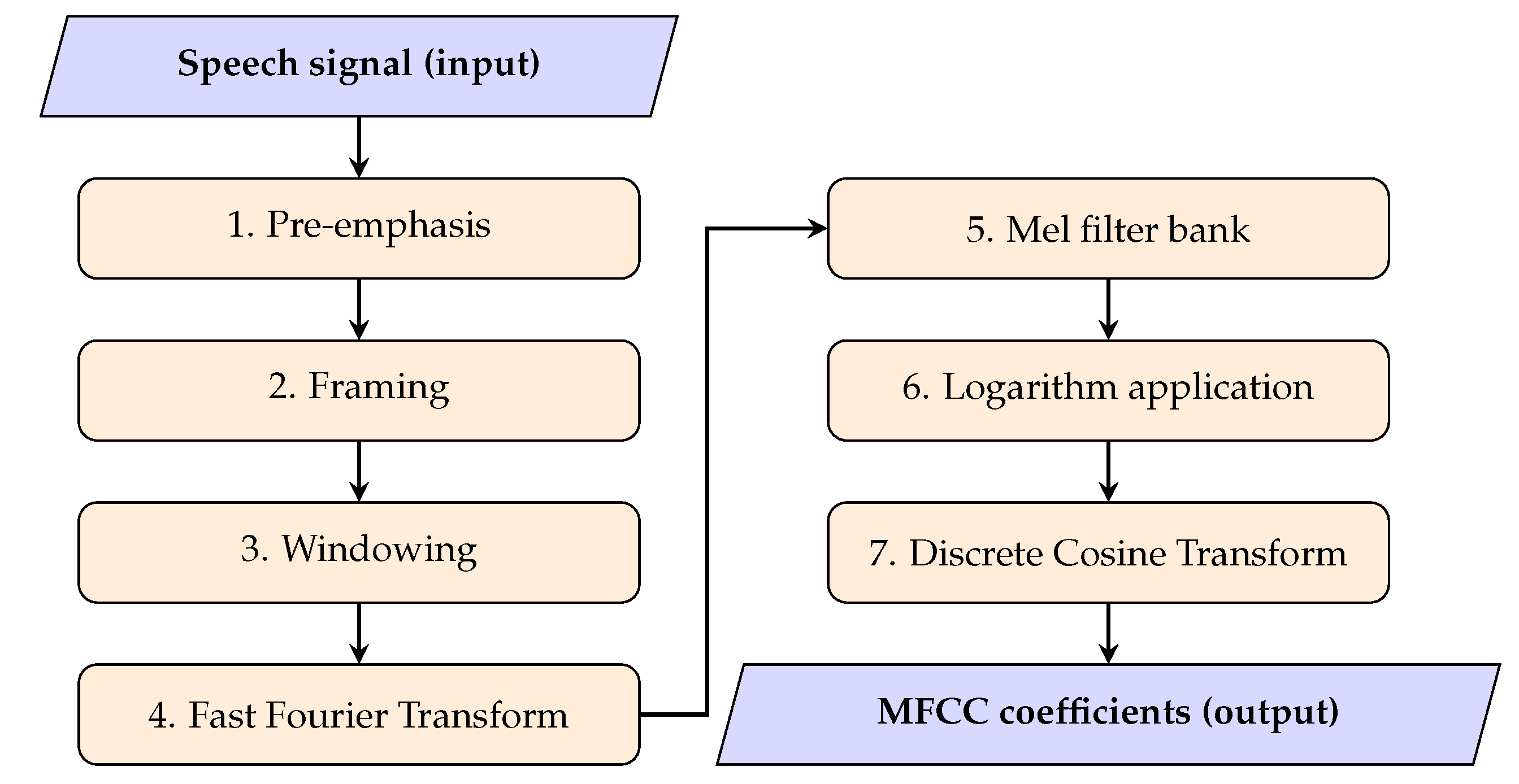
Figure 2.
Successive signal representations in the MFCC pipeline for a one-second speech-like signal (synthetic illustrative example; 16 kHz, 30 ms frames with 20 ms shift, 40 Mel filters, 13 coefficients): (a) raw waveform; (b) log-Mel spectrogram; (c) resulting MFCC matrix used as the two-dimensional network input.
Figure 2.
Successive signal representations in the MFCC pipeline for a one-second speech-like signal (synthetic illustrative example; 16 kHz, 30 ms frames with 20 ms shift, 40 Mel filters, 13 coefficients): (a) raw waveform; (b) log-Mel spectrogram; (c) resulting MFCC matrix used as the two-dimensional network input.
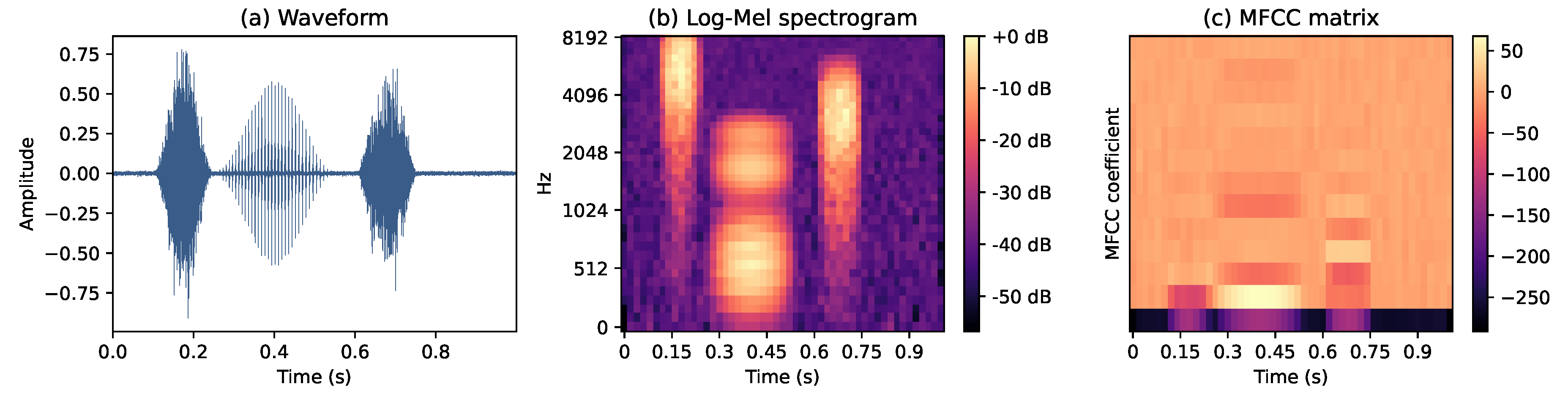
Figure 3.
Architecture of the proposed CNN model, read as a two-column fold from top to bottom. The left column is a convolutional feature extractor that applies three successive 2D convolutional layers (16, 8, and 5 filters) to the MFCC input and downsamples them with max-pooling. The right column flattens the resulting feature maps and classifies them through two fully connected layers, terminating in a 25-unit Softmax output, one per keyword class.
Figure 3.
Architecture of the proposed CNN model, read as a two-column fold from top to bottom. The left column is a convolutional feature extractor that applies three successive 2D convolutional layers (16, 8, and 5 filters) to the MFCC input and downsamples them with max-pooling. The right column flattens the resulting feature maps and classifies them through two fully connected layers, terminating in a 25-unit Softmax output, one per keyword class.
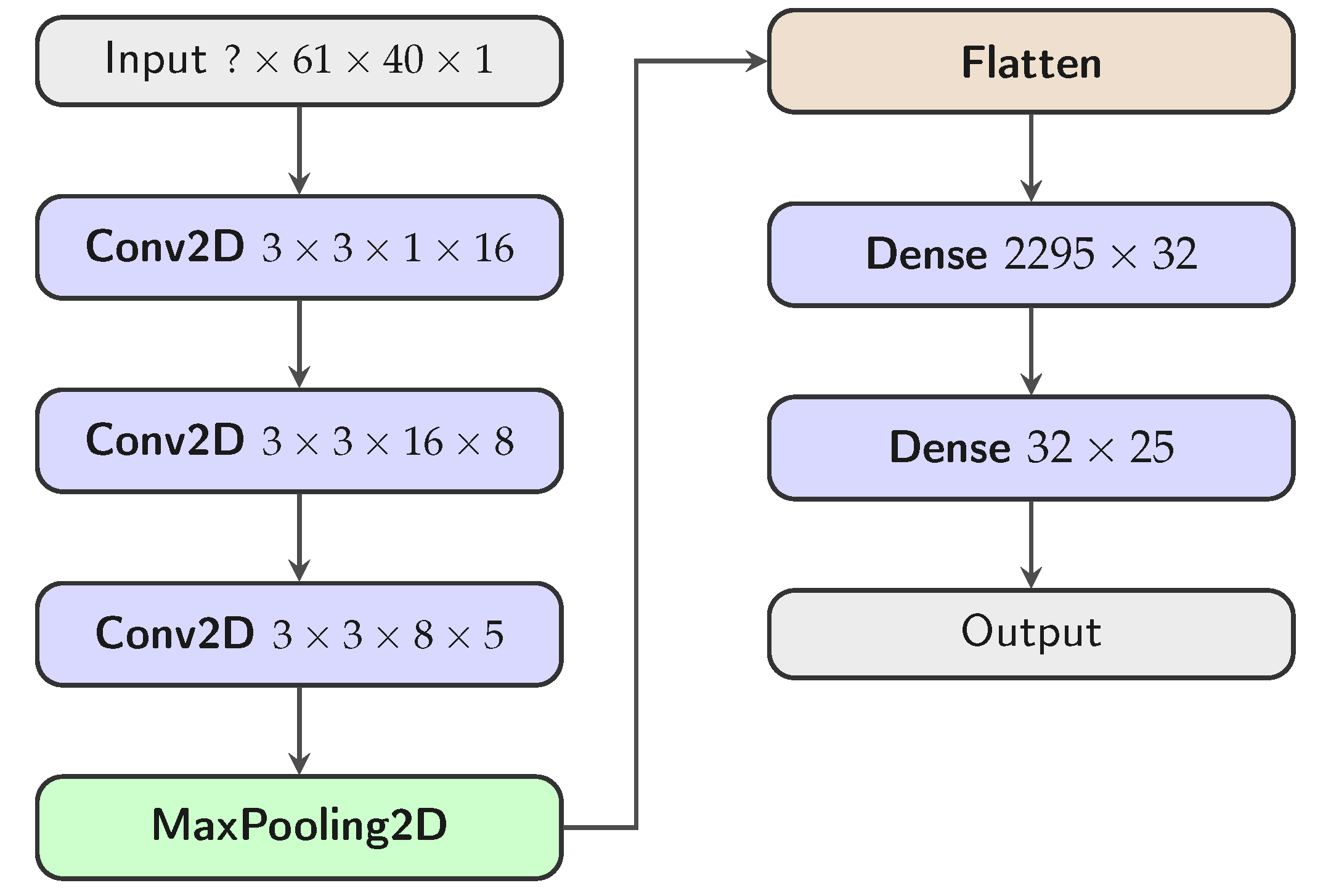
Figure 4.
Architecture of the proposed CRNN model. The left column is a convolutional front-end (Conv2D followed by max-pooling) that reduces the MFCC input; the feature maps are then reshaped into a time series and passed to the right column, where a single 32-unit GRU layer models the temporal dependencies of speech before a 25-unit Softmax classification layer produces the per-keyword probabilities.
Figure 4.
Architecture of the proposed CRNN model. The left column is a convolutional front-end (Conv2D followed by max-pooling) that reduces the MFCC input; the feature maps are then reshaped into a time series and passed to the right column, where a single 32-unit GRU layer models the temporal dependencies of speech before a 25-unit Softmax classification layer produces the per-keyword probabilities.
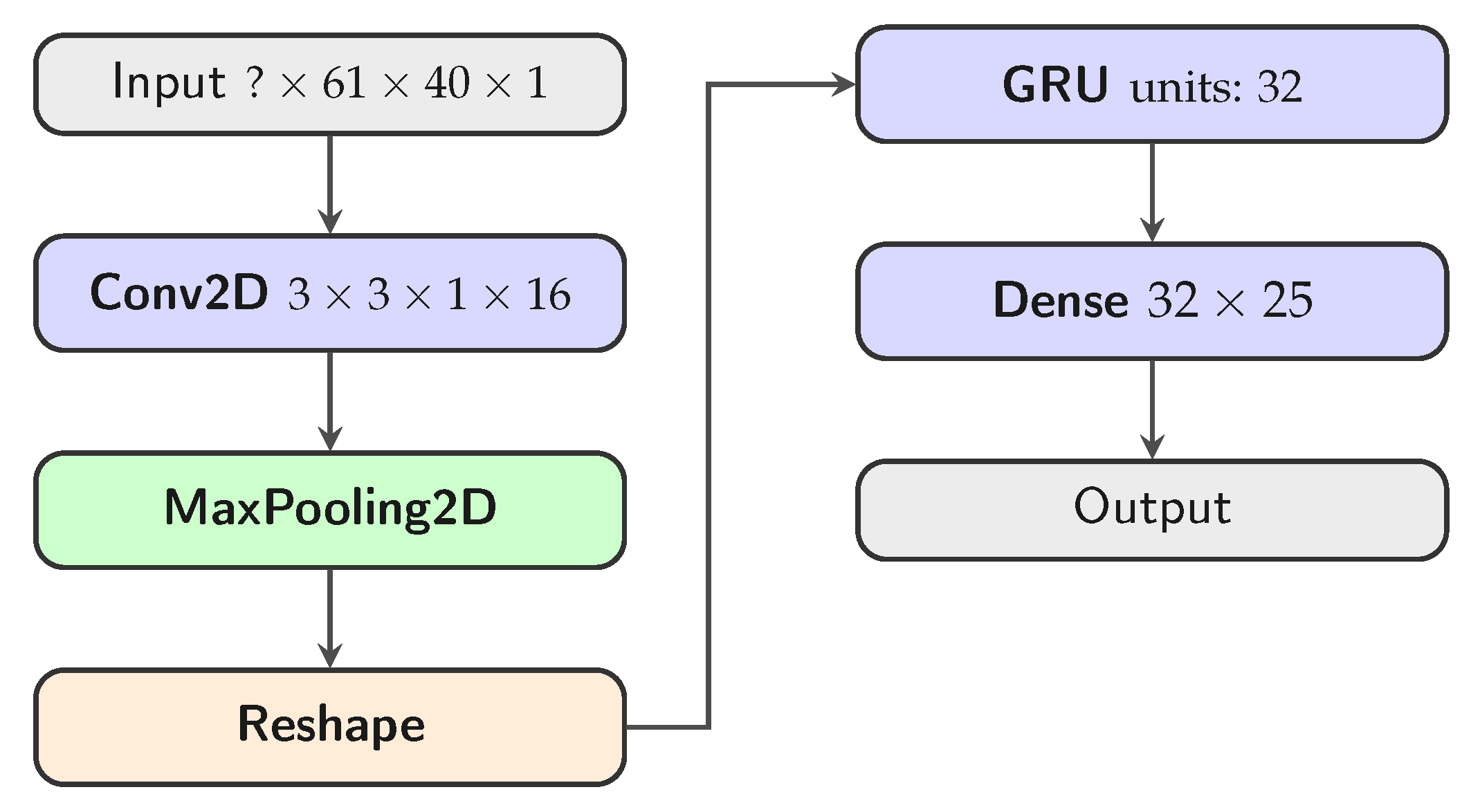
Figure 5.
Internal structure of a single depthwise-separable (DS) block, which factorizes a standard convolution into two phases. In the depthwise phase (left, blue), a kernel filters each input channel independently; in the pointwise phase (right, orange), a convolution linearly combines the channels into the output feature maps. Each phase is followed by Batch Normalization and a ReLU activation.
Figure 5.
Internal structure of a single depthwise-separable (DS) block, which factorizes a standard convolution into two phases. In the depthwise phase (left, blue), a kernel filters each input channel independently; in the pointwise phase (right, orange), a convolution linearly combines the channels into the output feature maps. Each phase is followed by Batch Normalization and a ReLU activation.
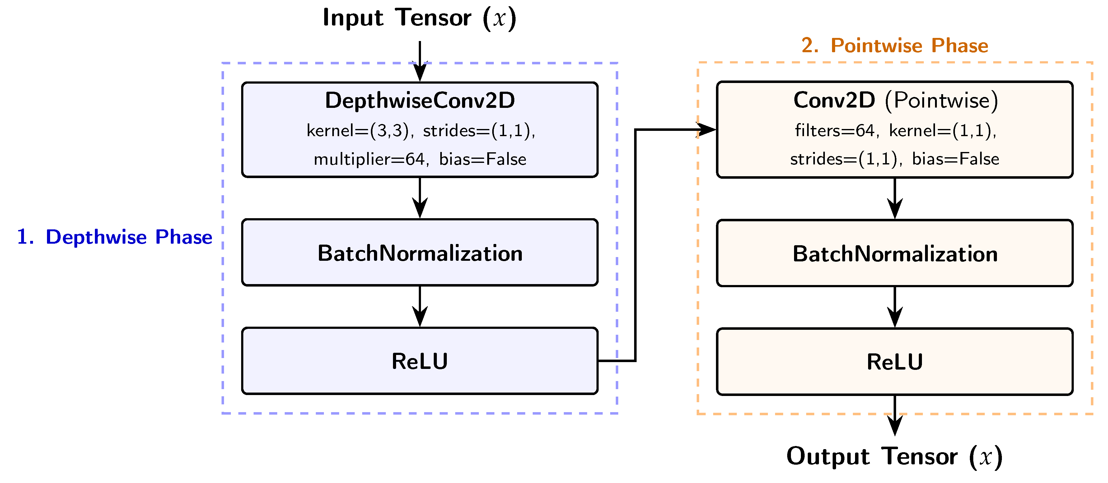
Figure 6.
Architecture of the proposed DS-CNN model, shown folded across two columns. An initial standard convolution (stem) processes the MFCC input, after which four stacked depthwise-separable blocks (DS Blocks 1–4, each detailed in Figure 5) extract features. The final feature maps are aggregated by global average pooling and mapped to the 25 keyword classes by a Softmax-activated dense layer.
Figure 6.
Architecture of the proposed DS-CNN model, shown folded across two columns. An initial standard convolution (stem) processes the MFCC input, after which four stacked depthwise-separable blocks (DS Blocks 1–4, each detailed in Figure 5) extract features. The final feature maps are aggregated by global average pooling and mapped to the 25 keyword classes by a Softmax-activated dense layer.
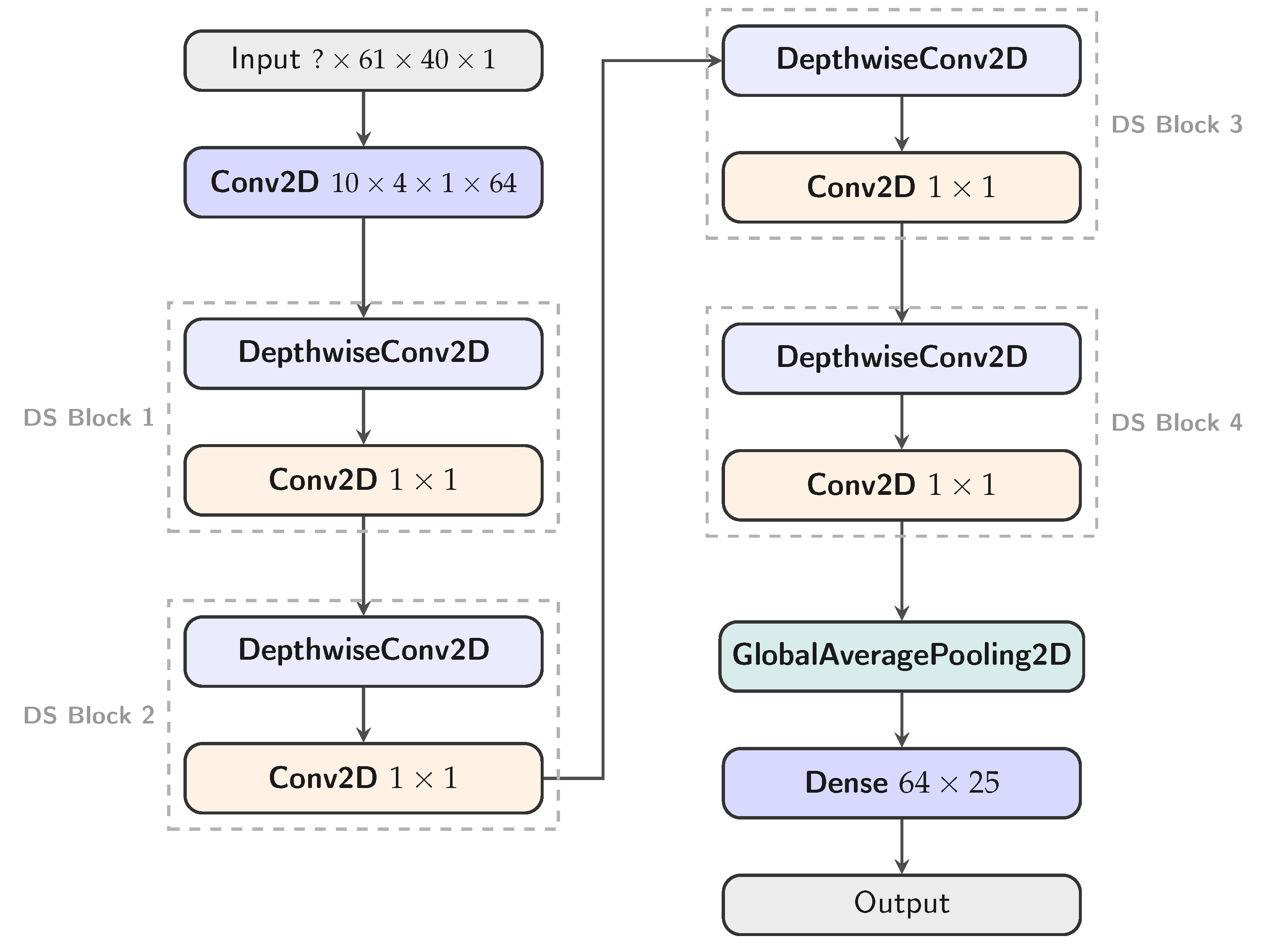
Figure 7.
PCB with Raspberry Pi Pico 2 microcontroller.
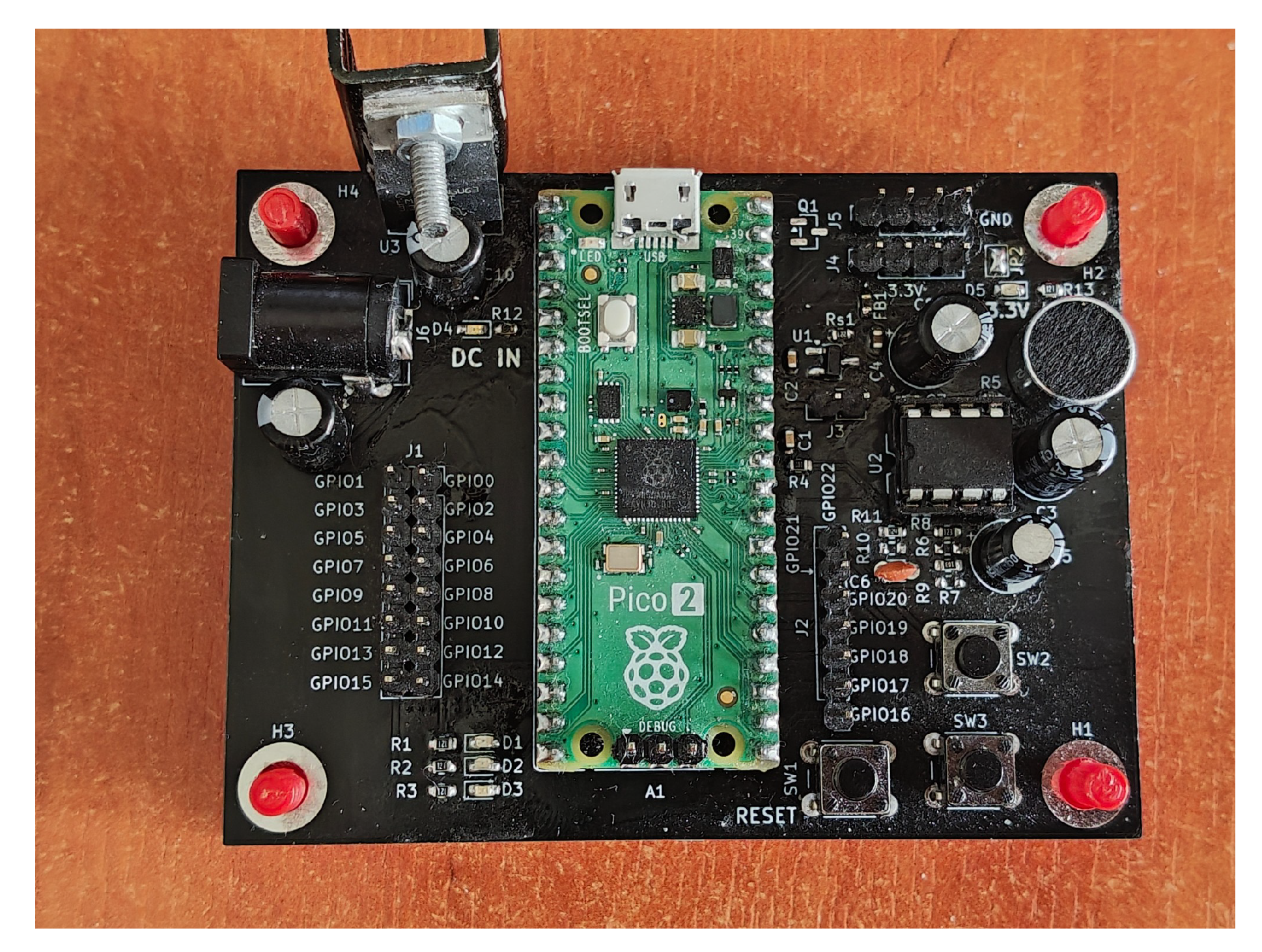
Figure 8.
Confusion matrices of the BC-ResNet model in (a) Float32 and (b) INT8 formats. Rows are the true classes and columns the predicted classes. The pronounced degradation of the keyword bird (ptak) under INT8 quantization is visible as a weakened diagonal entry.
Figure 8.
Confusion matrices of the BC-ResNet model in (a) Float32 and (b) INT8 formats. Rows are the true classes and columns the predicted classes. The pronounced degradation of the keyword bird (ptak) under INT8 quantization is visible as a weakened diagonal entry.
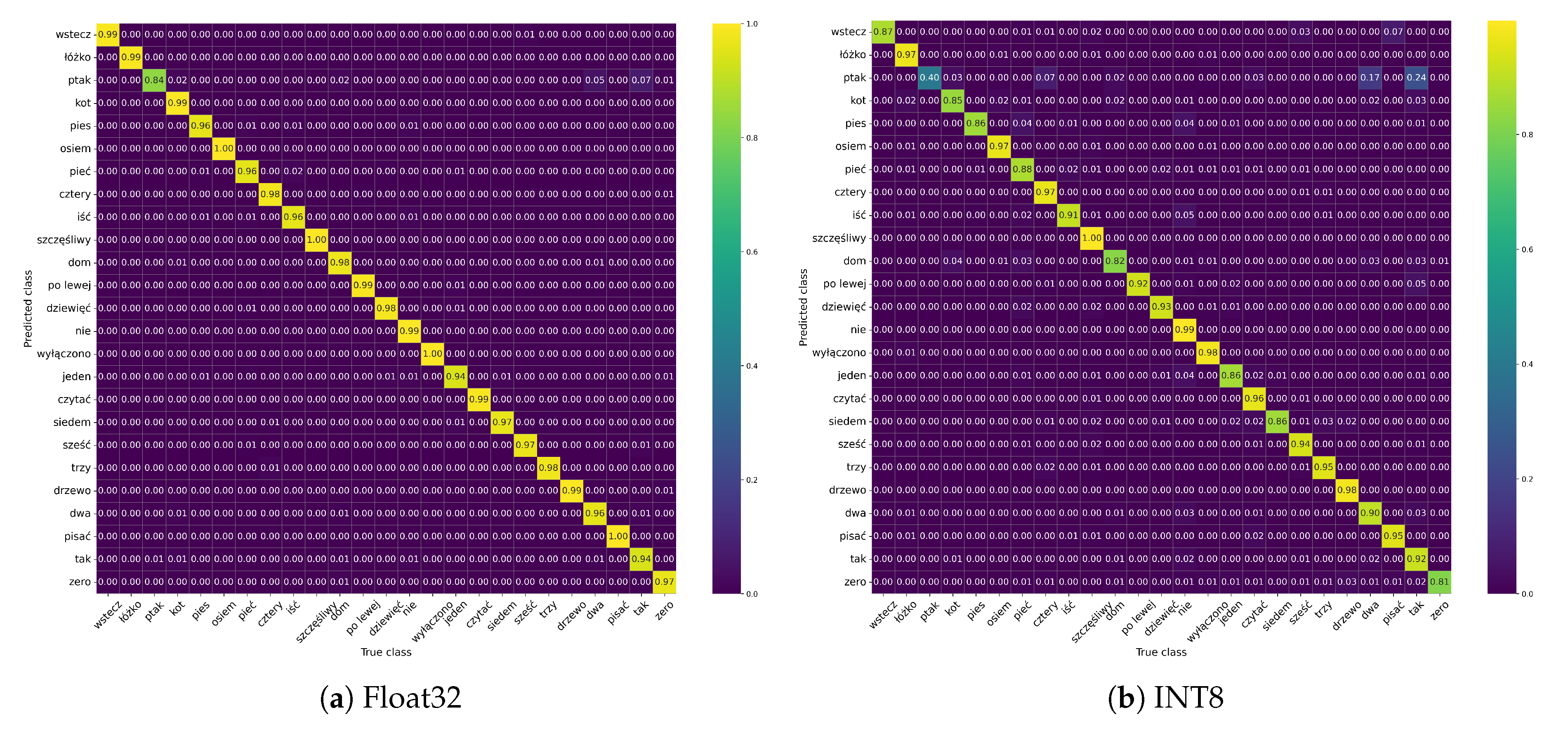

Table 1.
Summary of the total number of parameters (trainable and non-trainable) for the evaluated neural network architectures. BC-ResNet is included as a state-of-the-art reference architecture; the remaining three are the proposed designs.
Table 1.
Summary of the total number of parameters (trainable and non-trainable) for the evaluated neural network architectures. BC-ResNet is included as a state-of-the-art reference architecture; the remaining three are the proposed designs.
| Model Architecture | Number of Parameters |
|---|---|
| BC-ResNet | 13 450 |
| DS-CNN | 25 177 |
| CRNN | 33 433 |
| CNN | 75 982 |
Table 2.
List of Polish words used in experiments.
| Word (in English) | Word (in Polish) | Count |
|---|---|---|
| backward | wstecz | 918 |
| bed | łóżko | 4908 |
| bird | ptak | 1224 |
| cat | kot | 4362 |
| dog | pies | 5152 |
| eight | osiem | 4884 |
| five | pięć | 5164 |
| four | cztery | 5086 |
| go | iść | 5130 |
| happy | szczęśliwy | 4902 |
| house | dom | 5004 |
| left | po lewej | 1020 |
| nine | dziewięć | 4896 |
| no | nie | 31 086 |
| off | wyłączono | 3236 |
| one | jeden | 5612 |
| read | czytać | 4882 |
| seven | siedem | 4986 |
| six | sześć | 5008 |
| three | trzy | 5266 |
| tree | drzewo | 4380 |
| two | dwa | 5320 |
| write | pisać | 4816 |
| yes | tak | 8480 |
| zero | zero | 5124 |
Table 3.
Performance of the evaluated models in Float32 (full-precision) format: classification accuracy, F1-score, model size, and mean on-device inference time on the Raspberry Pi Pico 2 (mean of 100 trials per model). The best value in each column is shown in bold.
Table 3.
Performance of the evaluated models in Float32 (full-precision) format: classification accuracy, F1-score, model size, and mean on-device inference time on the Raspberry Pi Pico 2 (mean of 100 trials per model). The best value in each column is shown in bold.
| Model | Accuracy (%) | F1-Score | Size (KB) | Inference time (ms) |
|---|---|---|---|---|
| BC-ResNet | 97.81 | 0.9780 | 104.98 | 579.1 |
| DS-CNN | 97.06 | 0.9707 | 98.85 | 1693.7 |
| CRNN | 96.19 | 0.9620 | 218.79 | 347.9 |
| CNN | 88.68 | 0.8869 | 300.64 | 357.7 |
Table 4.
Performance of the evaluated models after INT8 quantization: classification accuracy, F1-score, model size, and mean on-device inference time on the Raspberry Pi Pico 2 (mean of 100 trials per model). The best value in each column is shown in bold.
Table 4.
Performance of the evaluated models after INT8 quantization: classification accuracy, F1-score, model size, and mean on-device inference time on the Raspberry Pi Pico 2 (mean of 100 trials per model). The best value in each column is shown in bold.
| Model | Accuracy (%) | F1-Score | Size (KB) | Inference time (ms) |
|---|---|---|---|---|
| BC-ResNet | 92.73 | 0.9258 | 101.97 | 501.9 |
| DS-CNN | 93.13 | 0.9331 | 46.15 | 311.3 |
| CRNN | 94.28 | 0.9431 | 182.62 | 150.3 |
| CNN | 85.32 | 0.8542 | 79.44 | 107.5 |
Table 5.
Per-sample acoustic measurements obtained from the electret-microphone front-end recordings. SNR was estimated using the lowest-energy decile of frames as a noise-floor proxy. Roll-off denotes the highest frequency bin within of the spectral peak. No clipping was detected in any sample ().
Table 5.
Per-sample acoustic measurements obtained from the electret-microphone front-end recordings. SNR was estimated using the lowest-energy decile of frames as a noise-floor proxy. Roll-off denotes the highest frequency bin within of the spectral peak. No clipping was detected in any sample ().
| Word | Word (eng.) | RMS (dBFS) | SNR (dB) | Roll-off (Hz) |
|---|---|---|---|---|
| jeden | one | 1875 | ||
| dwa | two | 1109 | ||
| cztery | four | 1516 | ||
| pięć | five | 1898 | ||
| osiem | eight | 1586 | ||
| dziewięć | nine | 1719 | ||
| łóżko | bed | 742 | ||
| Mean ± SD |
Disclaimer/Publisher’s Note: The statements, opinions and data contained in all publications are solely those of the individual author(s) and contributor(s) and not of MDPI and/or the editor(s). MDPI and/or the editor(s) disclaim responsibility for any injury to people or property resulting from any ideas, methods, instructions or products referred to in the content. |
© 2026 by the authors. Licensee MDPI, Basel, Switzerland. This article is an open access article distributed under the terms and conditions of the Creative Commons Attribution (CC BY) license (http://creativecommons.org/licenses/by/4.0/).
Copyright: This open access article is published under a Creative Commons CC BY 4.0 license, which permit the free download, distribution, and reuse, provided that the author and preprint are cited in any reuse.