

Submitted:
04 July 2026
Posted:
07 July 2026
You are already at the latest version
Abstract
River–aquifer interactions play a significant role during floods, yet they are often simplified or neglected in hydrodynamic models. Horizontal infiltration across the riverbed and vertical infiltration through the floodplain jointly contribute to bank storage, delaying and attenuating flood waves. This study presents a conceptual numerical framework that couples 1D surface hydrodynamics, 2D groundwater flow, and a vertical infiltration module to represent these exchanges during overbank flooding. Applied to a simplified lowland river system, the model captures both lateral and vertical flux components and quantifies their contributions to flood wave attenuation. Our findings indicate that, in a 50-km river reach, vertical infiltration through the floodplain accounts for approximately 90% of total bank storage. Total bank storage can contribute up to 4.3% of flow attenuation and reduce peak river water levels by as much as 24 cm. These results highlight the substantial influence of bank storage on extreme flood events and underscore the importance of representing groundwater pathways in flood modelling. The proposed model provides a practical, process-based framework for representing bank storage through a two-way coupled surface water–groundwater formulation with a few physically based parameter set. By explicitly resolving the governing exchange processes, the model enables improved inclusion of bank storage dynamics in flood modelling, while avoiding both simplified loss-type formulations and the complexity of fully multidimensional coupled SW–GW models.
Keywords:
floodplain infiltration
; bank storage
; numerical modelling
; flood attenuation
; surface–groundwater coupling
1. Introduction
Numerous studies have examined surface–groundwater interactions and the hydraulic gradients induced by rising river stages (e.g., [1,2]). Extreme flooding can lead to surface water infiltration, both vertically (across the ground surface) and horizontally (through the riverbed) [3]. Previous studies have investigated key controls on floodplain recharge, including bank slope, capillary effects, flood duration, and surface clogging layers [4,5,6]. These works demonstrated the importance of variably saturated flow and vertical infiltration processes, particularly in wide, gently sloping floodplains. However, these investigations omitted the consideration of bank storage effects on the river flood wave.
Surface–groundwater interaction models often neglect unsaturated floodplain processes. [7,8] reviewed strategies of coupling surface and groundwater models. Many river models offer only a crude approximation of infiltration through the riverbed and floodplain as a one-way loss rather than a dynamic exchange. For instance, the HEC-RAS software [9] has incorporated infiltration methods like Green-Ampt since version 6.0; however, its emphasis is on hydrological rainfall-runoff modelling rather than detailed consideration of subsurface interactions. Conversely, groundwater-oriented models often simplify the physics and the discretization of surface hydrodynamics. In MODFLOW, river–aquifer exchange is handled via streamflow packages such as SFR2, which employ a kinematic wave formulation for the river and restricts its representation to single grid cells (SFR2, [10]), preventing the application of different saturation conditions within the same river cross-section, such as within the floodplain. Furthermore, the kinematic wave equation fails to capture flood hysteresis.
Analytical mechanistic approaches allow for an inexpensive computation of surface–groundwater interaction and are in principle well suited for parameter-scarce representation of bank storage sought here, see e.g., [2] for a review. However, for the general case when riverbed leakage and floodplain infiltration coexist, mass conservation is difficult to ensure without complicated branching and iterations. A more universal method must rely on numerical modelling.
Fully integrated numerical modelling systems such as MIKE SHE [11] provide comprehensive coupling of surface flow, unsaturated flow, and groundwater dynamics, but at the expense of high data requirements and computational complexity, which may be unnecessary when the primary objective is to resolve bank storage dynamics during flood events. Other coupled approaches (e.g., [12,13,14]) demonstrate improved representation of floodplain infiltration but either neglect lateral unsaturated flow, simplify surface ponding processes, or require extensive parameterization.
In this paper, a simple mechanistic model is proposed to address this gap. The model integrates a one-dimensional (1D) surface water model (SWM) based on the full Saint-Venant equations, a horizontally two-dimensional (2DH) groundwater model (GWM) formulated from Darcy’s law and the continuity equation, and a zero-dimensional Vertical infiltration model (VIM) describing vertical infiltration across the inundated floodplain. Implemented within a finite-difference scheme for an idealized compound cross-section fully connected to an unconfined aquifer, the model captures the dominant processes governing bank storage and floodplain infiltration during flood events. The present study focuses exclusively on an event-based modelling of overbank flood conditions and the associated infiltration processes. Low-flow conditions and continuous modelling were not investigated. By relying on simplified yet physically consistent components, the framework provides a parsimonious representation of river–floodplain interactions while retaining two-way feedback between surface water and groundwater. A key characteristic of the framework is the simultaneous treatment of infiltration across the riverbed and from inundated floodplain surfaces. Resolving these pathways independently makes it possible to evaluate their respective roles in groundwater recharge, bank-storage development, and flood-wave modification, without making a priori assumptions in the mechanistic model on which one dominates. The model thus provides a practical foundation for analysing event-based bank storage dynamics and for developing infiltration modules suitable for hydrodynamic river models.
2. Methodology
Within the numerical framework developed in this study, exchange fluxes between the river and the aquifer are separated into vertical and horizontal components. Vertical fluxes, denoted (dimension: L/T), represent infiltration from the floodplain surface, while horizontal fluxes, denoted (dimension: L/T), correspond to seepage through the riverbed. In the rising limb, when river stages ( river hydraulic head, dimension: L) exceed the bank elevation (, aquifer thickness, dimension: L), and an overbank flooding depth is formed ( dimension: L), both flux types occur simultaneously, resulting in groundwater head rise ( aquifer hydraulic head, dimension: L). Figure 1 illustrates the generalized model configuration underlying the formulation of these physical processes.
2.1. Surface Water Model (SWM).
SWM is governed by the full Saint-Venant equations in 1D:
where is time, is the distance along the river, is the wetted cross-sectional area perpendicular to the flow direction (dimension: L2), is the volumetric flow rate along the river (dimension: L3/T), and is the total specific flow rate into the aquifer (dimension: L2/T) calculated by coupling with the GWM and VIM.
The momentum equation that accommodates non-uniform velocity distribution across the cross-section reads [18]:
where is the momentum coefficient associated with velocity shear between the main channel and the floodplain [19], is the acceleration due to gravity, is the depth of the center of gravity of the cross-section, is the longitudinal bed slope. The friction slope is calculated as:
The conveyance factor (dimension: L3/T) for the th part of the cross section is expressed with the Manning formula:
where is the length of the wetted perimeter between bed and water, the wetted cross-sectional area, and the Manning’s roughness coefficient (dimension: T L-1/3), all associated with the th part. Index refers to the left floodplain, the main channel, and the right floodplain, respectively. As to the momentum coefficient, it is computed as (see e.g., [20]):
2.2. Groundwater Model (GWM)
Darcy’s law governs fluid flow through porous media and, combined with mass conservation, yields the partial differential equation describing groundwater flow in saturated medium [21]. Rivers and floodplains typically consist of permeable alluvial deposits (e.g., sands and gravels), enabling infiltration from the river into the aquifer through the riverbed. If the water table is free to rise or descend in an unsaturated zone, then the aquifer is modelled as unconfined. Otherwise, if the aquifer is saturated over the whole aquifer depth, then it is considered confined.
To maintain parsimony, the aquifer is treated as a homogeneous and isotropic medium, focusing on the macro-scale bank storage exchange and its resulting pressure wave propagation. For such an unconfined aquifer, the 2DH equation of saturated transient horizontal flow (Dupuit assumption) is:
where is the hydraulic head of groundwater measured from the bottom of the aquifer (dimension: L); is the horizontal hydraulic conductivity of the aquifer (dimension: L/T); is the unconfined specific yield (dimensionless); is the total flux (dimension: L/T); is the lateral distance from the river.
When the hydraulic head of the groundwater, , measured from the bottom of the aquifer, exceeds the height of ground surface, , then groundwater no longer flows across a variable thickness, but rather across the aquifer thickness. When this happens, the governing equations switch to those of a confined, homogeneous, isotropic aquifer:
where is the storativity (dimensionless), and is obtained with ; is the specific storage (dimension: L-1), is the transmissivity (dimension: L2/T) obtained as .
Many groundwater models assume instantaneous percolation from the soil surface to the water table, neglecting flow through the unsaturated zone. This simplification may misrepresent subsurface water distribution, particularly near rivers [22]. The present model explicitly accounts for unsaturated floodplain infiltration driven by overbank surface water levels by coupling a vertical infiltration model (VIM) with the SWM and GWM components.
2.3. Vertical Infiltration Model (VIM)
Infiltration models are typically derived from mass conservation and Darcy’s law, commonly assuming one-dimensional vertical flow, a sufficiently deep water table, negligible air-pressure effects, and monotonically increasing saturation [23]. Among available approaches, the Green–Ampt model [24] is widely used in practice [25]. It provides an analytical approximation of Richards’ equation for ponded infiltration into deep, homogeneous soils with uniform initial moisture, assuming a sharp wetting front and a piston-type saturation profile.
The Green–Ampt model approximates the vertical flux () as follows:
where (dimension: L/T) is the vertical saturated hydraulic conductivity, is the time-variable water depth above the soil surface, (dimension: L) is the capillary suction head at the wetting front, assumed to be constant and uniform over the depth and (dimension: L) is the time-varying depth of the wetting front below the surface. represents an effective hydraulic conductivity that accounts for the presence of a low-permeability surface cover or clogged layer commonly observed in riverbeds and floodplains (e.g., [5]). Vertical flow across this layer is explicitly represented by the Green–Ampt model, which is parameterized to describe infiltration through the cover layer.
The cumulative infiltration depth (, dimension: L) can be related to through mass conservation by:
where (dimension: L3L-3) is the moisture deficit, equal to the difference between the soil porosity and the initial volumetric water content , both assumed to be constant over the depth and in time.
Using (8) and the relationship between the infiltration rate and the cumulative infiltration, , the cumulative infiltration depth, , can be obtained implicitly by using iterative numerical methods or explicitly by using approximations.
2.4. Exchange Flows and Bank Storage
The coupling strategy revolves around the exchange of flows between surface water and groundwater. The infiltrated flow is split into a horizontal and a vertical component. Horizontal fluxes () are based on Darcy’s law and correspond to the fluxes across the riverbed layer. Vertical fluxes (), on the other hand, only come into play when the river levels exceed that of the river banks and are computed using the Green-Ampt model. The total specific flow from the river is decomposed as
where is the horizontal flux through the river bed (dimension: L/T); and is the wetted perimeter (dimension: L). is driven by the horizontal pressure gradient between the river and the groundwater as:
where is the hydraulic conductivity of the riverbed (dimension: LT-1); is the height of the river water surface above the aquifer bottom, calculated by the SWM (dimension: L); is the hydraulic head of the aquifer, calculated by the GWM (dimension: L); and is the riverbed layer thickness (dimension: L).
The hydraulic conductivity of the riverbed often differs from that of the adjacent aquifer due to surface processes such as colmation. Colmation occurs when fine particles become trapped within the pore spaces, reducing porosity and permeability and thereby decreasing riverbed hydraulic conductivity [26]. Conversely, when scouring occurs, it removes sediment and clears some of the clogged material from the colmated layer, resulting in greater and lower [27].
As to the last term, , the vertical flux (dimension: LT-1) is calculated through VIM Eq. (8) and it is integrated over the entire width of the active floodplain, . In the model presented in this paper, we assume that the soil under the floodplain is initially unsaturated, and during flood events, when the river inundates the floodplain, the ponding depth in the Green-Ampt model is equal to the local depth of the surface water above the floodplain soil, . As infiltration proceeds, the wetting front propagates downward until it reaches the groundwater table. At this point, the unsaturated zone between the floodplain surface and the groundwater table is fully saturated, and the fundamental assumptions of the Green–Ampt model are no longer satisfied because a distinct wetting front no longer exists. Consequently, the Green–Ampt formulation is replaced by a saturated Darcy-flow formulation, in which vertical infiltration is governed by the hydraulic gradient between the floodplain surface and the groundwater table:
where is the thickness of the soil layer beneath the floodplain (dimension: L).
Bank storage refers to the volume of water that infiltrates riverbanks and active floodplain soils. Bank storage is partitioned according to the origin of the inflow: denotes the volume infiltrated through vertical infiltration flow rate (), whereas represents the volume contributed by horizontal infiltration flow rate (). To quantify bank storage, the temporal evolution of specific bank storage is first computed for each transect by integrating the infiltration flow rate over the duration of the flood hydrograph. The peak value of specific bank storage is then identified for each transect. These peak values are subsequently integrated along a specified river reach to obtain reach-averaged peak specific bank storage components, and .
Due to the symmetric cross-sectional geometry and identical hydraulic properties prescribed for the left and right floodplains, bank-storage processes develop symmetrically on both sides of the river. The reported bank-storage volumes represent the combined contribution of both floodplains.
3. Numerical Solution
To obtain a numerical solution, the governing differential equations are discretized into a system of algebraic equations [28]. In this study, a finite difference method (FDM) is applied to a structured nodal grid, requiring the selection of appropriate approximations for the derivatives at the spatial and temporal grid points.
For the SWM, the Saint-Venant equations were solved using the explicit Lax scheme. Although implicit schemes are more efficient, explicit schemes are well-suited for handling nonlinearity and internal grid points, as noted by [29]. When applied in its general vector form, the approximations of the Lax scheme read:
The stabilizing parameter , serving as a weighting coefficient, is usually between 0 and 1. In our simulations, we found that a value of 1 yielded the most accurate and still stable solution, reducing the Lax method to the forward Euler one.
For the GWM, the equation for a 2D horizontal flow was approximated by using the central difference approximation to the second derivative for changes in space, and the forward Euler method in time.
For the VIM, a first-order numerical approximation was implemented using the explicit Euler method to solve eq. (8). This approach requires small time steps and a known initial condition for the cumulative infiltration variable, . The method demonstrated good agreement with results obtained from solving the Richards equation using the Hydrus-1D model [30] across a variety of soil types.
The VIM is initiated when the overbank water depth exceeds a minimum threshold, set to 1 cm in our simulations. At the onset of overbank flooding, the soil is assumed to be initially unsaturated, with an initial water content equal to the residual water content of the soil. The water deficit content is approximated to the specific yield () to maintain the continuity between the unsaturated zone and the unconfined aquifer. A limiting condition is imposed when the calculated vertical flux exceeds either the soil’s saturated vertical hydraulic conductivity or the rate of surface water level rise. Once the wetting front reaches the water table, the soil profile is considered saturated, and infiltration is subsequently calculated using the saturated Darcy flux (Eq. (11). The overlapping volume of soil between the wetting front and the water table is added as recharge to the GWM node.
After the overbank flood recedes, soil moisture is redistributed. This redistribution phase is modelled using the Green-Ampt Redistribution (GAR) approach, wherein the piston-like wetting front elongates due to unsaturated flow driven by capillary and gravitational forces. This redistribution process preserves a rectangular soil moisture profile and conserves water mass. As the depth to the wetting front () increases, the water content throughout the wetted zone is assumed to decrease uniformly [31,32].
A MATLAB [33] code was developed to solve the system of equations and calculate the exchange fluxes. It employs an explicit time-stepping procedure. The model advances a limited set of state variables in time, namely river hydraulic head and discharge for the SWM, hydraulic head for the GWM, and cumulative infiltration for the VIM. No additional state variable is introduced for the GAR; instead, infiltration fluxes are adjusted dynamically based on the interaction between and . All variables are updated explicitly at each time step without iterative convergence. The numerical structure of the SWM follows the explicit formulation proposed by [34].
4. Benchmark Problem
To evaluate the consistency of the developed framework, this section introduces a simplified benchmark problem. The primary objective of this application is to quantify the roles of horizontal and vertical infiltration in modifying flood wave propagation in a typical lowland river where the floodplain is constrained between levees.
The conceptual model comprises an unconfined aquifer bounded by a fully penetrating river. In this model, the aquifer is assumed to be homogeneous and transversely isotropic, with an impermeable horizontal base. The model does not account for rainfall infiltration or evapotranspiration. [13] demonstrated that simplifying hydraulic conductivity over a heterogeneous floodplain aquifer did not significantly degrade the simulation of hydraulic heads.
The surface and aquifer geometry are both prismatic, with a uniform longitudinal slope. The cross section of the river is the combination of a rectangular main channel and a symmetric, rectangular floodplain bounded by vertical levees. This is a reasonable simplification for many lowland river reaches, however, neglecting the lateral slope of the floodplain may be too crude for reaches that are laterally unconfined. Despite these simplifying assumptions, it is important to note that the numerical solver could be adapted to incorporate more complex features as needed. As an example, the aquifer models (GWM and VIM) can use a curvilinear grid fitted to the river centreline.
For this analysis, a 50 km reach was selected to provide a sufficiently long river segment for the development of cumulative flood-wave attenuation and river–floodplain exchange processes while remaining computationally efficient and relevant for reach-scale flood-management assessments.
Laterally, the aquifer domain extends much further than the levees, to give ample room to the propagation of the groundwater wave before it reaches the lateral boundaries (). A sensitivity analysis was performed on the grid parameters. The spatial resolution was defined with an anisotropic grid interval of = 1 km longitudinally and = 50 m laterally. Although this results in a relatively large cell aspect ratio, the choice reflects the different spatial scales of the simulated processes. Longitudinal variations in river stage and groundwater heads occur gradually along the river reach, whereas the dominant groundwater gradients develop in the transverse direction between the river and the floodplain. A grid-sensitivity analysis was conducted using longitudinal cell sizes of 2000, 1000, and 500 m and transverse cell sizes of 100, 50, and 25 m. The results indicated that river discharge, river depth, infiltrated fluxes, and bank-storage volumes were only weakly affected by further refinement. Although temporal infiltration fluxes were somewhat more sensitive to the transverse discretization, the solutions converged as decreased. Therefore, the adopted discretization was considered sufficient to accurately represent the coupled processes while maintaining reasonable computational requirements.
The time step used is = 1s, which is smaller than the maximum time step permitted by the Courant stability condition. This conservative choice was made to ensure numerical stability of the explicit SWM.
In the SWM, the boundary condition at the upstream boundary is a discharge hydrograph given as a discrete time series. A steady-state equilibrium (normal flow) is used as initial condition. The outflow boundary condition is the normal flow depth corresponding to the computed discharge assuming an unchanged bed slope. The wetted area was calculated through explicit extrapolation of zero order, i.e., , where 1 denotes the first node of the x-axis (input), 2 is the node closest to the input (within the domain), denotes the current time, and denotes the previous time. The area was extrapolated at the outflow boundary, and the water level was calculated from the discharge by assuming normal flow [35].
In the GWM, the initial condition for the aquifer is obtained from a steady-state solution, and no-flow boundary conditions are applied in the groundwater domain.
The case study presented here idealizes the lower reach of the Danube River in Hungary, between the municipalities of Dunaújváros and Mohács (rkm 1580–1446). The active floodplain area covers approximately 108 km2 on the left bank and 140 km2 on the right bank. Given the 135 km length of this river reach, the average floodplain width is estimated at 785 m on the left bank and 1020 m on the right bank, resulting in an average total width of 1805 m. For modelling purposes, a symmetric channel cross-section was adopted, with a representative floodplain width of 900 m on each side. The 2013 flood hydrograph was used as boundary inflows. The maximum discharge of 9080 m3/s occurred on 10 June 2013.
The river reach under study is bordered by sandy and gravel aquifers [35,36,37,38,39], which supports the assumption of relatively uniform hydraulic properties across all three case studies. To account for the spatial variability and uncertainty of soil conductivity, the hydraulic conductivity was varied by discretizing its order of magnitude into three scenarios (SCN25 to SCN27) for the Danube. The selected conductivity range (5–500 m d−1) spans values typically associated with fine sand, medium to coarse sand, and gravelly sand deposits, thereby representing a broad range of hydraulic conditions within sandy alluvial floodplain sediments rather than fundamentally different soil types.
Table 1 lists the principal model parameters used in this hypothetical river-aquifer system.
Verification of the SWM was conducted for a 1D river model through HEC-RAS 6.3.1 [9]. The VIM was verified for a single soil profile column using Hydrus-1D 4.17 [41]. The GWM was verified using a 2D domain through MODFLOW-2005 [42]. While the accuracy of each model can be assessed independently, the evaluation of the combined system relies on mass conservation and stability.
5. Numerical Sensitivity Analysis
This section presents a sensitivity analysis to evaluate the influence of key numerical choices and physical assumptions on the modelled flood attenuation and the volume of bank storage.
5.1. Infiltration Methods
As an alternative approach to the unsaturated Green–Ampt method (Eq. (8) and (9)), a saturated Darcy-based approach was also evaluated for estimating vertical infiltration fluxes. Whereas the Green–Ampt method switches to the saturated Darcy equation Eq. (12) only when the aquifer is fully saturated, this alternative Darcy-based approach uses Eq. (12) at all times.
When modelling a real river, the GWM and the VIM would usually be calibrated to match observed groundwater levels or estimated bank storage volumes. Here, to ensure consistency between the two VIM methods, the Darcy-based approach was calibrated to reproduce the same mean vertical infiltration flux as the Green–Ampt model by adjusting the equivalent clogging-layer thickness.
Once this flux-equivalence was ensured, the choice between the two VIM methods produced minimal differences in bank storage, as expected. Total specific bank storage (BST) differed by less than 1% when calculated with the Green–Ampt method compared to the Darcy-based approach, for the three scenarios (SCN25 to SCN27), over 50 km.
Flood attenuation metrics ( and ) are evaluated 50 km downstream of the inflow boundary. Discharge attenuation () defined as the relative attenuation of peak discharge, showed only minor differences: the Green–Ampt method produces slightly higher attenuation in the low-conductivity case (SCN25, 0.6% of difference between the two methods), but slightly lower values in the medium- (SCN26, 0.7%) and high-conductivity (SCN27, 0.3%) scenarios. Variations in river water depth between the upstream and downstream sections remained small, with absolute differences between the two infiltration formulations remaining within approximately 0.07 (SCN27) to 0.16 cm (SCN25).
The primary differences between the two formulations emerge in the temporal dynamics of infiltration. The Green–Ampt model produces 3.7% to 24.8% higher peak vertical volumetric flow rates and advances hydrograph peaks by approximately 1 to 8 hours at the downstream section (50 km). This reflects the strong initial hydraulic gradients associated with infiltration into an initially unsaturated soil profile.
5.2. Vertical and Horizontal Infiltration Processes
The model’s sensitivity to disabling vertical () or horizontal () fluxes was evaluated under low- (SCN25) and high-conductivity (SCN27) scenarios. Disabling led to a substantial reduction in BST, decreasing from 1016 x103 to 200 x103 m3/km (an 80% drop) in SCN25, and from 2575 x103 to 1452 x103 m3/km (44%) in SCN27. In comparison, disabling produced a much smaller impact: BST decreased to 1013 x103 m3/km (0.3%) in SCN25 and to 2574 x103 m3/km (0.04%) in SCN27.
changed by less than 1% when no was evaluated, and by 12% (SCN25) and 7% (SCN27) when no was evaluated. Disabling barely increased from 20.80 cm to 20.87 cm (+0.35%) in the low- conductivity scenario (SCN25), and from 23.59 cm to 24.06 cm (+2%) in the high-conductivity scenario (SCN27). Conversely, disabling consistently reduced in both cases (-14% in SCN25; -11% in SCN27).
5.3. 1D and 2D Lateral Groundwater Flow
The model’s sensitivity to the dimensionality of lateral groundwater flow was evaluated under low (SCN25) and high (SCN27) hydraulic conductivity conditions. A one-dimensional (1D) lateral flow configuration was implemented by removing -direction flow from the groundwater flow equations (Eq. (6) and (7)), thereby allowing lateral flow only, i.e., in the -direction. The results showed that the model was largely insensitive to the switching between 2D and lateral 1D groundwater flow formulations, with negligible differences observed in river flow and bank storage.
5.4. Boundary Effects
To reduce the error in the simulated flood attenuation caused by the normal-depth downstream boundary condition, the model domain was extended with a buffer reach downstream of the 50-km-long study reach. This commonly applied approach ensures that the boundary condition does not artificially constrain flood-wave hysteresis of the SWM to a fixed stage–discharge relationship.
A sensitivity analysis performed using progressively longer longitudinal domains ( = 75, 150, 300, and 600 km) revealed a considerable sensitivity to the extension length. The 600 km simulation was adopted as the reference solution. Within the 50 km upstream study reach, relative differences in peak discharge were 0.8%, 0.32% and 0.05%, whereas absolute differences in peak river water depth were 0.5 m, 0.2 m, 0.01 m for = 75, 150, 300 km, respectively. Since the computational cost was not a limiting factor, the 600 km domain was finally retained to minimize potential downstream boundary effects on flood attenuation.
6. Results
In this section, the numerical solutions are evaluated for the benchmark problem by simulating a flood event with overbank flow. The instantaneous volumetric flow rates and were first averaged at each transect over the simulation period, considering only time steps with non-zero fluxes. These transect-scale averages were then spatially aggregated along a 50 km river reach to derive reach-scale volumetric flow metrics, resulting in specific flow components, and .
Bank-storage dynamics were quantified by computing the time evolution of specific bank storage at each transect, obtained by integrating the local specific infiltration flux over the duration of the flood hydrograph. For each transect, the peak specific bank-storage value was identified and subsequently integrated along a 50-km reach to derive reach-averaged peak bank-storage components, and . A summary of these results is provided in Table 2.
The dominance of over primarily reflects the large floodplain width relative to the main channel in this simulation and the stronger hydraulic gradients that develop across the floodplain compared with those near the riverbank.
6.1. Flow and Stage Hydrograph
Figure 2 presents the inflow and outflow hydrographs along the 50-km river reach, together with the vertical (), horizontal (), and total () volumetric flow rates for three representative scenarios: SCN25 (low hydraulic conductivity), SCN26 (medium conductivity), and SCN27 (high conductivity).
To examine the spatiotemporal evolution of groundwater response during the flood event, Figure 3 shows the simulated hydraulic-head variations at two representative lateral distances from the river channel: 50 m (near the river bank) and 900 m (at the levee position).
Although the near-river response at 50 m is similar among the three scenarios, slight differences are observed during the early flooding stage. The lower-conductivity scenario (SCN25) shows a faster local head increase, because water remains concentrated near the river bank due to slow lateral groundwater movement, whereas in the higher conductivity (SCN27), infiltrated water redistributes quickly laterally through the aquifer.
At 900 m, the abrupt increase in corresponds to the moment when the wetting front reaches the groundwater table, causing the previously unsaturated soil column to become fully saturated. Therefore, this jump should not be interpreted as the arrival of the lateral groundwater pressure wave at the levee. Instead, it reflects the transition from partially saturated to fully saturated conditions, which produces a sudden increase in the lateral groundwater gradient and, consequently, in hydraulic head at that location. The earlier occurrence of this transition in SCN26 and SCN27 indicates faster vertical infiltration and saturation under higher hydraulic conductivity, while in SCN25 this process is delayed.
6.2. Flood Attenuation
Compared with the no-infiltration scenario, where flood attenuation resulted only from surface storage , the inclusion of infiltration and the associated bank-storage processes produced additional attenuation across all hydraulic conductivity scenarios. Attenuation increased to 3.9% in the low-conductivity case (SCN25), 3.8% in the medium-conductivity case (SCN26), and 4.3% in the high-conductivity case (SCN27). This corresponds to an additional attenuation effect of 0.5, 0.4, and 0.9%, respectively, attributable to river–aquifer exchange. Relative to the no-infiltration scenario , the average peak water depth reduction between the upstream and downstream sections was in SCN25, in SCN26, and in SCN27. Thus, infiltration and bank storage contributed additional reductions of approximately 3.2 cm, 3.1 cm, and 6.0 cm, respectively.
7. Discussion
Hydrodynamic models typically neglect river–aquifer interactions or represent them as simplified loss terms without groundwater feedback. Although several studies have addressed this limitation through coupled surface water–groundwater modelling, many rely on restrictive assumptions, such as neglecting groundwater feedback [12,14], prescribing ponding conditions independently of overbank flooding [43], or focusing on dryland environments [15]. Fully integrated frameworks based on Richards-equations formulations, such as the MIKE SHE model [11], and UZF1 package [15] for MODFLOW, provide detailed representations of surface flow, variably saturated flow, and groundwater dynamics. However, their application to large river–floodplain systems is often limited by substantial computational requirements [17], and the need for extensive parametrization of unsaturated-zone hydraulic properties. In contrast, the formulation adopted here captures the dominant controls on infiltration capacity and wetting-front propagation using a simplified parameterization while avoiding the iterative nonlinear solution procedures required by Richards-equation models. Although the proposed approach cannot resolve detailed moisture profiles within the vadose zone, the results suggest that it is sufficient for estimating reach-scale bank storage, floodplain recharge, and flood-wave attenuation, which are the primary objectives of the present study.
Within this context, the proposed framework explicitly couples river hydraulics, groundwater flow, and infiltration through an initially unsaturated floodplain. A distinguishing feature of the approach is the explicit separation of horizontal riverbed exchange and vertical floodplain infiltration, allowing their individual contributions to bank storage and flood-wave attenuation to be quantified.
The benchmark simulations consistently identified inundated floodplain surfaces as the primary source of groundwater recharge during flood events (86–87% of total exchange and about 90% of bank storage), whereas seepage through the riverbed contributed only a comparatively small fraction of the total exchange volume Sensitivity analyses further confirmed this result: suppressing riverbed exchange produced only minor changes in attenuation, whereas removing floodplain infiltration substantially reduced both bank storage and flood attenuation. This differs from many conventional river–aquifer models that represent exchange exclusively through horizontal hydraulic gradients between the river and aquifer (e.g., [22,44,45]), suggesting that neglecting floodplain infiltration may lead to underestimation of bank storage and attenuation, particularly in wide floodplains subjected to prolonged inundation.
Comparison of the Green–Ampt and Darcy-based formulations showed similar cumulative bank-storage volumes and flood attenuation over the analysed reach, indicating that the choice of infiltration model primarily affects transient dynamics rather than cumulative exchange. These findings contrast with [5], who reported lower bank-storage volumes when the unsaturated zone was represented explicitly, but is consistent with studies showing that vadose-zone processes mainly influence recharge timing rather than total recharge [15,16]. The Green–Ampt formulation provides a more physically realistic representation of transient infiltration, particularly during the early stages of flooding and in the presence of the 2–3 m unsaturated zone observed in the Danube floodplains, but requires additional parameters and increases sensitivity to vadose-zone properties. In contrast, the Darcy-based formulation is computationally simpler and may be sufficient for estimating cumulative recharge, bank storage, and flood attenuation at the reach scale, whereas explicit unsaturated formulations become more important when transient infiltration dynamics and hydrograph timing are of primary interest, such as in flood forecasting applications.
Negligible differences were observed between 1D and 2DH groundwater representations, indicating that longitudinal (river-aligned) groundwater gradients were of secondary importance relative to lateral exchange in the investigated configurations. Consequently, groundwater flow can be simplified to a lateral 1D representation in this case without significant loss of accuracy, supporting earlier findings (e.g., [16,43,44]) and offering practical means of reducing computational complexity in large-scale applications. However, this simplification may not be appropriate for systems characterized by strong longitudinal gradients, meandering channels, tributary confluences, or other complex hydraulic settings.
Although vertical infiltration dominated in the investigated configuration, this conclusion should not be generalized to all river–floodplain systems, as infiltration dynamics are strongly influenced by additional factors such as flood duration and soil hydraulic properties. For instance, if a long-duration flood occurs over soils with low infiltration capacity—or conversely, if the flood hydrograph is short—then infiltration losses may be negligible [14]. In contrast, under conditions of higher permeability or prolonged inundation, infiltration can substantially affect flood wave propagation. In the asymptotic case of vanishing floodplain width, the present model reverts to a classical Darcy model coupled horizontally with the river model [22,44,45].
For further applications, the framework offers a practical means of incorporating bank-storage processes into flood analyses without requiring fully integrated surface–subsurface simulations. This makes it attractive for screening studies, conceptual investigations, and river-management assessments where computational efficiency is an important consideration.
8. Conclusion
This study presented a coupled surface–subsurface numerical model for simulating river–aquifer interactions during overbank flooding. The model combines the 1D Saint-Venant equations, a 2DH groundwater formulation, and a modified Green–Ampt infiltration model. This combination explicitly represents both horizontal riverbed exchange and vertical infiltration through an initially unsaturated floodplain. The framework enables the evaluation of bank-storage dynamics and flood-wave attenuation in river–floodplain systems.
Application to a benchmark problem representative of the record 2013 flood on the lower Hungarian reach of the Danube showed that vertical floodplain infiltration is the dominant exchange pathway, largely due to the broad floodplain and steep hydraulic gradients in the initially unsaturated soil. In contrast, riverbed exchange contributed only marginally to the overall recharge process. Neglecting vertical infiltration reduced simulated bank storage and flood attenuation, highlighting the importance of explicitly representing floodplain recharge during overbank flooding.
Comparison of alternative vertical infiltration formulations (Green–Ampt and Darcy-based approaches) and groundwater dimensionality (laterally 1D and 2DH representations) demonstrated that simplified formulations can adequately reproduce reach-scale bank storage and flood attenuation while reducing computational and calibration requirements. These findings support the use of parsimonious modelling approaches for event-scale analyses of river–aquifer interactions in large river–floodplain systems.
From a practical perspective, the proposed framework provides a practical tool for investigating floodplain infiltration, bank storage, and flood-wave attenuation lowland rivers. The explicit representation of both riverbed exchange and floodplain infiltration enables direct quantification of their relative contributions to recharge and attenuation, while maintaining a computational cost suitable for long river reaches and extensive sensitivity analyses. The framework is therefore particularly useful for preliminary assessments of river–aquifer interactions and for applications where detailed characterization of unsaturated-zone hydraulic properties is unavailable. Future work could incorporate spatially variable soil properties, clogging temporal dynamics, evapotranspiration, successive flood waves, low-flow conditions, and more detailed vadose-zone representations to further improve realism and applicability.
Acknowledgments
This work was carried out as part of studies supported by the Stipendium Hungaricum Scholarship through the Hungarian Government’s initiative, administered via the Tempus Public Foundation; G.F,F. thanks the program for the opportunity. Furthermore, this research was funded by the Ministry of Culture and Innovation and the National Research, Development and Innovation Office under Grant Nr. TKP2021-NVA-02.
References
- Cranswick, R. H., Cook, P. G. “Scales and magnitude of hyporheic, river-aquifer and bank storage exchange fluxes”, Hydrological Processes, 29(14), pp. 3084–3097, 2015. [CrossRef]
- Ferraz, G., Krámer, T. “Surface Water–Groundwater Interactions and Bank Storage during Flooding: A Review”, Periodica Polytechnica Civil Engineering, 66(1), pp. 149–163, 2022. [CrossRef]
- Bates, P. D., Stewart, M. D., Desitter, A., Anderson, M. G., Renaud, J. P., Smith, J. A. “Numerical simulation of floodplain hydrology”, Water Resources Research, 36(9), pp. 2517–2529, 2000. [CrossRef]
- Li, H., Boufadel, M. C., Weaver, J. W. “Quantifying bank storage of variably saturated aquifers”, Groundwater, 46(6), pp. 841–850, 2008. [CrossRef]
- Doble, R.C., R.S. Crosbie, B.D. Smerdon, L. Peeters, F.J. Cook. “Groundwater recharge from overbank floods”, Water Resources Research, 48(9), 2012. [CrossRef]
- Doble, R., Brunner, P., McCallum, J., Cook, P. G. “An analysis of river bank slope and unsaturated flow effects on bank storage”, Groundwater, 50(1), pp. 77-86, 2012. [CrossRef]
- Haque, A., Salama, A., Lo, K., Wu, P. “Surface and groundwater interactions: a review of coupling strategies in detailed domain models”, Hydrology, 8(1), pp. 35, 2021. [CrossRef]
- Ntona, M. M., Busico, G., Mastrocicco, M., Kazakis, N. “Modeling groundwater and surface water interaction: An overview of current status and future challenges”, Science of The Total Environment, 846, 157355, 2022. [CrossRef]
- U.S. Army Corps of Engineers, Hydrologic Engineering Center, “HEC-RAS (Version 6.3.1)”, [computer program] Available at: https://www.hec.usace.army.mil/confluence/rasdocs/rasrn/6.3.1 [Accessed: 01 March 2026].
- Niswonger, R. G., Prudic, D. E. “Documentation of the Streamflow-Routing (SFR2) Package to include unsaturated flow beneath streams — A modification to SFR1”. U.S. Geological Survey Techniques and Methods, book 6, chap. A13. 50 p., 2005. Available at: https://pubs.usgs.gov/publication/tm6A13 [Accessed: 01 March 2026].
- DHI. “MIKE SHE User Guide and Reference Manual”, Available at: https://manuals.mikepoweredbydhi.help/latest/MIKE_SHE.htm [Accessed: 01 March 2026].
- Saksena, S., Merwade, V., Singhofen, P. J. “Flood inundation modeling and mapping by integrating surface and subsurface hydrology with river hydrodynamics”. Journal of Hydrology, 575, 1155-1177, 2019. [CrossRef]
- Bernard-Jannin, L., Brito, D., Sun, X., Jauch, E., Neves, R., Sauvage, S., Sánchez-Pérez, J.-M. “Spatially distributed modeling of surface water–groundwater exchanges during overbank flood events: A case study at the Garonne River”. Advances in Water Resources, 94, pp. 146–159, 2016. [CrossRef]
- Hou, J., Zhang, Z., Zhang, D., Shi, B., Chen, G., Zhang, H. “Study on the influence of infiltration on flood propagation with different peak shape coefficients and duration”, Water Policy, 23(4), pp. 1059-1074, 2021. [CrossRef]
- Niswonger, R. G., Prudic, D. E., Regan, R. S. “Documentation of the unsaturated-zone flow (UZF1) package for modeling unsaturated flow between the land surface and the water table with MODFLOW-2005”. U.S. Geological Survey, 2006. Retrieved May 20, 2021, from https://pubs.usgs.gov/tm/2006/tm6a19/pdf/tm6a19.pdf.
- Costa, A. C., Bronstert, A., De Araújo, J. C. “A channel transmission losses model for different dryland rivers”. Hydrology and Earth System Sciences, 16(4), pp. 1111-1135, 2012. [CrossRef]
- Farthing, M.W., Ogden, F.L. “Numerical Solution of Richards’ Equation: A Review of Advances and Challenges”, Soil Science Society of America Journal, 81: 1257-1269, 2017. [CrossRef]
- Rashid, R. M., Chaudhry, M. H. “Flood routing in channels with flood plains”, Journal of Hydrology, 171(1-2), pp. 75-91, 1995. [CrossRef]
- Chen, Z., Chen, Q., Jiang, L. “Determination of apparent shear stress and its application in compound channels”, Procedia Engineering, 154, pp. 459-466, 2016. [CrossRef]
- Chow, V. T. “Open-channel hydraulics”, McGraw-Hill civil engineering series, 1959. ISBN: 07-010776-9.
- Freeze, R. A., Cherry, J. A. “Equations of Groundwater Flow”, In Groundwater, Prentice-hall, 1979, pp 63-69. ISBN: 0133653129.
- Moench, A. F., Barlow, P. M. “Aquifer response to stream-stage and recharge variations. I. Analytical step-response functions”, Journal of Hydrology, 230(3-4), pp. 192-210, 2000. [CrossRef]
- Mishra, S. K., Tyagi, J. V., Singh, V. P. “Comparison of infiltration models”, Hydrological Processes, 17(13), pp. 2629-2652, 2003. [CrossRef]
- Green, W. H., Ampt, G. A. “Studies on soil physics, 1: The flow of air and water through soils”. J. Agric. Sci., 4(1), pp. 1–24, 1911.
- Kale, R. V., Sahoo, B. “Green-Ampt infiltration models for varied field conditions: A revisit”. Water Resources Management, 25, pp. 3505-3536, 2011. [CrossRef]
- Veličković, B. “Colmation as one of the processes in interaction between the groundwater and surface water”. Facta Universitatis-series: Architecture and Civil Engineering, 3(2), pp. 165-172, 2005. https://doiserbia.nb.rs/img/doi/0354-4605/2005/0354-46050502165V.pdf.
- Levy, J., Birck, M. D., Mutiti, S., Kilroy, K. C., Windeler, B., Idris, O., Allen, L. N. “The impact of storm events on a riverbed system and its hydraulic conductivity at a site of induced infiltration”, Journal of Environmental Management, 92(8), pp. 1960-1971, 2011. [CrossRef]
- Ferziger, J. H., Perić, M., Street, R. L. “Computational methods for fluid dynamics”, Springer, 2019. ISBN 978-3-319-99691-2. [CrossRef]
- Chanson, H. “Explicit finite difference methods”, In Environmental hydraulics for open channel flows, Elsevier, 2004, pp 306-312. ISBN: 0750661658.
- Šimůnek, J., van Genuchten, M. T., Sejna, M. “Development and applications of the HYDRUS and STANMOD software packages and related codes”. Unsaturated zone journal, 7(2), pp. 587-600, 2008. [CrossRef]
- Ogden, F. L., Saghafian, B. “Green and Ampt infiltration with redistribution”, Journal of Irrigation and Drainage Engineering, 123(5), pp. 386-393, 1997. [CrossRef]
- Lai, W., Ogden, F. L., Steinke, R. C., Talbot, C. A. “An efficient and guaranteed stable numerical method for continuous modeling of infiltration and redistribution with a shallow dynamic water table”, Water Resources Research, 51(3), pp. 1514-1528, 2015. [CrossRef]
- MathWorks. “MATLAB (Version 9.10.0.1684407, R2021a Update 3)”, [computer program] Available at: https://www.mathworks.com/products/matlab.html [Accessed: 01 March 2026].
- Simões, A.L.A., Schulz, H. E., Porto, R. M. “Métodos computacionais em hidráulica” [Computational Methods in Hydraulics], EDUFBA, 2017. ISBN 978-85-232-1602-3. Available at: https://repositorio.ufba.br/handle/ri/23994. (in Portuguese).
- Gama, I. R. V., Simões, A. L. A., Schulz, H. E., De Melo Porto, R. “Código livre para solução numérica das equações de saint-venant em canais trapezoidais assimétricos” [Open-source code for the numerical solution of the Saint-Venant equations in asymmetric trapezoidal channels], Revista Eletrônica de Gestão e Tecnologias Ambientais, pp. 145-159, 2020. (in Portuguese).
- Ubell, K. “Surface- and groundwater relationships along the Hungarian reach of the Danube River”, In: Symposium surface waters hold at the occasion of general assembly of Berkeley of IUGG, vol. 19, no. 31.8. 1963.
- Kolencsik-Tóth, A., Kovács, B. “Calibration process for groundwater flow model of a river influenced shallow aquifer”, Central European Geology, 58(1-2), pp. 186-198, 2015. [CrossRef]
- Murinkó, G., Bene, K. “Hydrologic modeling of the loess bluff in Dunaujvaros, Hungary”, Pollack Periodica, 12(1), pp. 3-15, 2017. [CrossRef]
- Trásy, B., Magyar, N., Havril, T., Kovács, J., Garamhegyi, T. “The Role of Environmental Background Processes in Determining Groundwater Level Variability—An Investigation of a Record Flood Event Using Dynamic Factor Analysis”, Water, 12(9), 2336, 2020. [CrossRef]
- Wagner, F., Csoma, R. “A felszín alatti áramlás és árhullámok kapcsolatának vizsgálata változó folyami vízszintek esetében” [Investigating groundwater flow regime and flood waves in case of different water levels], Hidrológiai Közlöny, 102(3), pp. 50-60, 2022. (in Hungarian).
- PC Progress. “Hydrus-1D (Version 4.17)”, [computer program] Available at: https://www.pc-progress.com/en/Default.aspx?H1d-downloads [Accessed: 01 March 2026].
- Harbaugh, A. W. “MODFLOW-2005, the US Geological Survey modular ground-water model: the ground-water flow process (Vol. 6)” Reston, VA, USA: US Department of the Interior, US Geological Survey, 2005.
- Rassam, D. W., Pickett, T., Knight, J. H. “Incorporating floodplain groundwater interactions in river modeling”, In: 18th World IMACS/MODSIM Congress, Cairns, Australia, 2009, pp. 3116–3122. ISBN: 978-0-9758400-7-8. Available at https://mssanz.org.au/modsim09/I1/rassam.pdf.
- Pinder, G. F., Sauer, S. P. “Numerical simulation of flood wave modification due to bank storage effects”, Water Resources Research, 7(1), 63–70, 1971. [CrossRef]
- Whiting, P. J., Pomeranets, M. “A numerical study of bank storage and its contribution to streamflow”, Journal of Hydrology, 202(1–4), 121–136, 1997. [CrossRef]
Figure 1.
Lateral view (Y-Z axes) containing the composite river section (main channel and floodplain), showing the notation used in this paper.
Figure 1.
Lateral view (Y-Z axes) containing the composite river section (main channel and floodplain), showing the notation used in this paper.
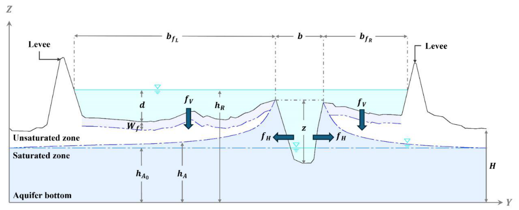
Figure 2.
Inflow (), outflow (), on the left axis, and horizontal (), vertical (), and total () infiltrated volumetric flow rate hydrographs, integrated over the length, on the right axis, within 50-km river reach, for scenario (a) SCN25, (b) SCN26, and (c) SCN27. is the time at the onset of overbank flooding, the time of peak overbank flow, and the end of overbank flood. Across all scenarios, is initiated early in the simulation within the saturated riverbed layer. In contrast, begins only once river water overtops the banks (namely at ), allowing floodwater to percolate vertically through the initially unsaturated floodplain soil. A distinct peak appears at the onset of overbank flooding, driven by the steep hydraulic gradient toward the dry vadose zone. As this zone becomes saturated, vertical infiltration rates progressively decline. The duration of unsaturated infiltration decreases with increasing hydraulic conductivity, reflecting the more rapid saturation of highly permeable soils. After the flood recedes and overbank flow ceases, vertical infiltration terminates, and directed toward the river develops, caused by the reversal of the hydraulic gradient between the aquifer and the river channel.
Figure 2.
Inflow (), outflow (), on the left axis, and horizontal (), vertical (), and total () infiltrated volumetric flow rate hydrographs, integrated over the length, on the right axis, within 50-km river reach, for scenario (a) SCN25, (b) SCN26, and (c) SCN27. is the time at the onset of overbank flooding, the time of peak overbank flow, and the end of overbank flood. Across all scenarios, is initiated early in the simulation within the saturated riverbed layer. In contrast, begins only once river water overtops the banks (namely at ), allowing floodwater to percolate vertically through the initially unsaturated floodplain soil. A distinct peak appears at the onset of overbank flooding, driven by the steep hydraulic gradient toward the dry vadose zone. As this zone becomes saturated, vertical infiltration rates progressively decline. The duration of unsaturated infiltration decreases with increasing hydraulic conductivity, reflecting the more rapid saturation of highly permeable soils. After the flood recedes and overbank flow ceases, vertical infiltration terminates, and directed toward the river develops, caused by the reversal of the hydraulic gradient between the aquifer and the river channel.
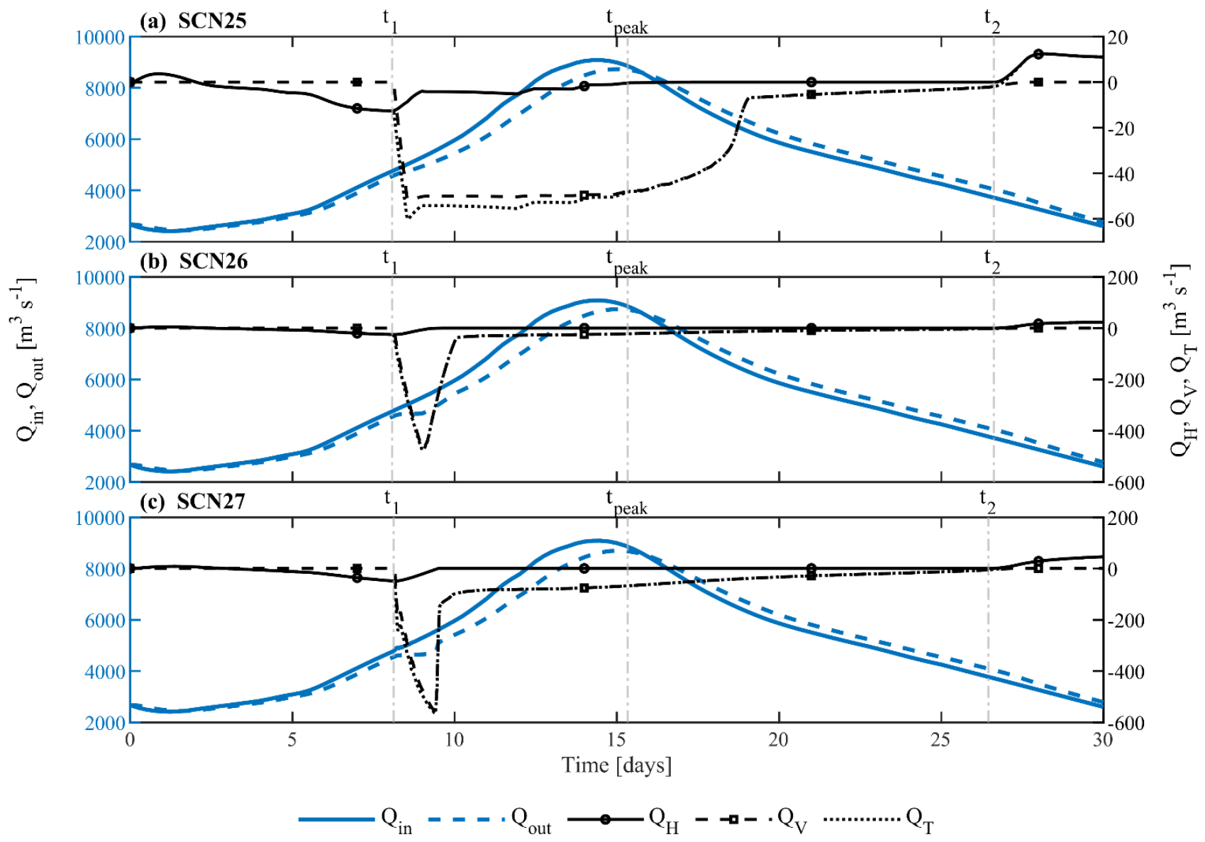
Figure 3.
Temporal evolution of river head (), groundwater head (), and wetting front head (), at two representative lateral distances from the river channel: 50 m (near the river bank) and 900 m (at the levee position), for scenarios (a) SCN25, (b) SCN26, and (c) SCN27. All plots correspond to the outflow cross section, located 50 km from the inflow boundary condition. The comparative analysis of scenarios SCN25–SCN27 highlights the controlling role of hydraulic conductivity in governing river–aquifer interactions during overbank flooding. In the low-conductivity case (SCN25), infiltration through the unsaturated zone progresses slowly, producing delayed and attenuated groundwater responses, especially at greater distances from the channel, indicating limited hydraulic connectivity and greater resistance to flow. As conductivity increases (SCN26), groundwater responses become faster and more pronounced, reflecting more efficient hydraulic transmission and earlier saturation of the vadose zone. In the highest-conductivity scenario (SCN27), saturation occurs rapidly after the onset of overbank flooding, and groundwater heads rise nearly in phase with the river stage throughout the floodplain. Although a brief period of unsaturated infiltration still occurs, it is quickly overtaken by saturated flow as the soil column becomes fully saturated. The near-synchronous head rise and substantial groundwater response observed even at 900 m from the river demonstrate strong hydraulic connectivity and minimal resistance to lateral flow within the aquifer.
Figure 3.
Temporal evolution of river head (), groundwater head (), and wetting front head (), at two representative lateral distances from the river channel: 50 m (near the river bank) and 900 m (at the levee position), for scenarios (a) SCN25, (b) SCN26, and (c) SCN27. All plots correspond to the outflow cross section, located 50 km from the inflow boundary condition. The comparative analysis of scenarios SCN25–SCN27 highlights the controlling role of hydraulic conductivity in governing river–aquifer interactions during overbank flooding. In the low-conductivity case (SCN25), infiltration through the unsaturated zone progresses slowly, producing delayed and attenuated groundwater responses, especially at greater distances from the channel, indicating limited hydraulic connectivity and greater resistance to flow. As conductivity increases (SCN26), groundwater responses become faster and more pronounced, reflecting more efficient hydraulic transmission and earlier saturation of the vadose zone. In the highest-conductivity scenario (SCN27), saturation occurs rapidly after the onset of overbank flooding, and groundwater heads rise nearly in phase with the river stage throughout the floodplain. Although a brief period of unsaturated infiltration still occurs, it is quickly overtaken by saturated flow as the soil column becomes fully saturated. The near-synchronous head rise and substantial groundwater response observed even at 900 m from the river demonstrate strong hydraulic connectivity and minimal resistance to lateral flow within the aquifer.
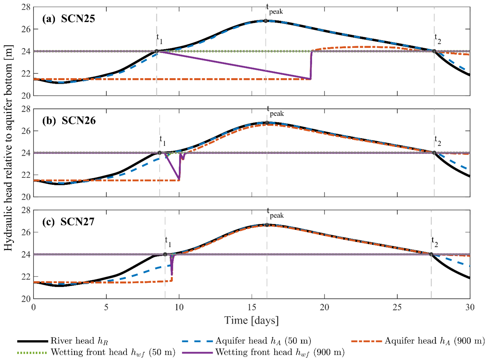

Table 1.
Hydraulic parameters and their values used in the model, for the Danube River between the municipalities of Dunaújváros and Mohács.
Table 1.
Hydraulic parameters and their values used in the model, for the Danube River between the municipalities of Dunaújváros and Mohács.
| Parameter | Value | Unit |
|---|---|---|
| 475 | m | |
| 9 | m | |
| cm km-1 | ||
| 0.033 | s m-1/3 | |
| 0.1 | s m-1/3 | |
| 1800 | m | |
| 0.15 | d-1 | |
| 0.21 | - | |
| m-1 | ||
| SCN25: 5 SCN26: 50 SCN27: 500 |
m d-1 | |
| SCN25: 0.5643 SCN26: 0.3020 SCN27: 0.1598 |
m | |
| 0.21 | - | |
| SCN25: 0.15 SCN26: 1.5 SCN27: 15 |
d-1 | |
| (2013) | 9080 | m3 s-1 |
| (2013) | 16.0 | d |
| 4575 | m3 s-1 |
Table 2.
Vertical and horizontal components of the specific infiltration flux from the river into the aquifer (, , ), averaged over the duration of the flood simulation. The corresponding maximum bank-storage volumes (, , ), for all scenarios. All the variables are averaged over a 50 km river length.
Table 2.
Vertical and horizontal components of the specific infiltration flux from the river into the aquifer (, , ), averaged over the duration of the flood simulation. The corresponding maximum bank-storage volumes (, , ), for all scenarios. All the variables are averaged over a 50 km river length.
| Scenario | [d-1] | [m/d] | Mean [m3/s/km] | Mean [m3/s/km] | Mean [m3/s/km] | Max [103 m3/km] | Max [103 m3/km] | Max [103 m3/km] |
|---|---|---|---|---|---|---|---|---|
| SCN25 | 0.15 | 5 | 0.56 | 0.09 | 0.65 | 910 | 106 | 1016 |
| (86%) | (14%) | (90%) | (10%) | |||||
| SCN26 | 1.5 | 50 | 0.82 | 0.12 | 0.94 | 1310 | 121 | 1431 |
| (87%) | (13%) | (92%) | (8%) | |||||
| SCN27 | 15 | 500 | 1.50 | 0.23 | 1.73 | 2348 | 227 | 2575 |
| (87%) | (13%) | (91%) | (9%) |
Disclaimer/Publisher’s Note: The statements, opinions and data contained in all publications are solely those of the individual author(s) and contributor(s) and not of MDPI and/or the editor(s). MDPI and/or the editor(s) disclaim responsibility for any injury to people or property resulting from any ideas, methods, instructions or products referred to in the content. |
© 2026 by the authors. Licensee MDPI, Basel, Switzerland. This article is an open access article distributed under the terms and conditions of the Creative Commons Attribution (CC BY) license (http://creativecommons.org/licenses/by/4.0/).
Copyright: This open access article is published under a Creative Commons CC BY 4.0 license, which permit the free download, distribution, and reuse, provided that the author and preprint are cited in any reuse.


