

Submitted:
06 July 2026
Posted:
07 July 2026
You are already at the latest version
Abstract
Handheld Mobile Laser Scanning (HMLS) is increasingly used for high resolution 3D mapping in construction, mining and natural environments. This study evaluates the strengths and limitations of HMLS for vegetation assessment in diverse tropical eco-systems across north Queensland, Australia, including rangelands, grasslands, man-groves and estuarine wetland forests. We assessed the accuracy of HMLS-derived point clouds against ground-truth measurements and compared performance with UAV SfM–MVS surveying. HMLS achieved centimeter-level accuracy for vegetation metrics, with mean absolute errors of 8.5 cm for Diameter at Breast Height (DBH) in rangeland forests and 6.7 cm for tussock height. The system consistently produced high-density point clouds, enabling detailed characterization of vertical structure, particularly understory vegetation often obscured in aerial surveys. HMLS proved operationally flexible across closed-canopy wetlands, mangroves, rangeland forests and open grasslands. Key limi-tations included restricted horizontal point cloud penetration in dense vegetation, compounded by access constraints and environmental conditions, and point cloud drift in areas with few geometric features, such as grasslands, which introduced uncertainty in vegetation metrics. High computational demands further constrained workflow effi-ciency. Overall, HMLS demonstrates strong potential as an accurate and versatile tool for vegetation mapping and structural analysis in complex tropical ecosystems.
Keywords:
handheld mobile laser scanner (HMLS)
; mobile LiDAR
; vegetation structure
; biomass estimation
; mangroves
; wetlands
; rangelands
; point cloud
1. Introduction
Tropical regions, encompassing mangroves, wetlands, and rangelands, play crucial roles in climate regulation, biodiversity, ecological services, and carbon sequestration. Tropical ecosystems contain approximately 25% of global terrestrial carbon and account for 34% of Earth’s gross primary production [1]. Mangrove forests, for example, store three to four times more carbon when compared to terrestrial forests, by trapping carbon rich particles in their above and below ground biomass [2,3,4]. Coastal wetlands cover approximately 9% of Earth’s surface, and are among the planet’s most valuable ecosystems, providing essential services including biodiversity services, water quality improvement, flood abatement, carbon sequestration, nutrient processing, and coastal protection, with an estimated annual economic value of $20.4 trillion per year, highlighting their significant contribution to environmental and societal well-being [5,6]. Rangelands, while often overlooked in carbon accounting, due to lower carbon storage density despite covering about half of Earth’s surface, still store greater than 10% of terrestrial carbon, and up to 30% of global soil organic carbon [7,8,9]. Furthermore, rangelands play major roles in supporting animal production, providing about 70% of forage for domestic livestock, which support livelihoods of approximately one billion people in tropical developing countries with 180 million people in Africa alone [10,11,12].
Vegetation biomass refers to the total amount of plant material within an ecosystem and is a critical indicator of ecosystem health, linking climate regulation with carbon storage. Biomass is categorised into above-ground biomass (AGB) and below-ground biomass (BGB). AGB refers to the total mass of living plant matter above the soil surface, typically including stems, leaves, branches, flowers, fruits, whereas BGB refers to the total mass of living plant matter beneath the soil surface, primarily roots. Each play distinct roles in carbon sequestration; for instance, AGB typically constitutes the largest carbon pool in African tropical rainforests, while BGB can represent over 40% of total carbon stocks in Brazilian tropical wet grasslands [13,14,15,16,17]. Accurate measurements of biomass are essential for translating biomass data into carbon stock estimates, minimising errors in carbon cycle assessments, and informing effective policy and greenhouse gas management [18,19]. Furthermore, effective management and monitoring of biomass are crucial for climate change mitigation and for supporting ecosystem productivity, biodiversity conservation, carbon sequestration, and ecological resilience [20,21,22,23]. Australian ecosystems face unique challenges in accurately modelling biomass specifically due to ecosystem high heterogeneity, sensor limitations, and a lack of standardised methods [24]. Addressing these challenges when collecting vegetation data is essential for effectively monitoring and managing biomass, which supports carbon accounting, conservation efforts, and sustainable land management practices [20,21,22,23].
AGB estimations can be calculated from measured structural vegetation proxies: DBH, height, and volume [25,26,27]. Various methods for collecting structural proxies, including traditional field measurements, airborne platforms, and satellite-based remote sensing, have contributed to ecological research on vegetation structure, biomass, species composition, and ecosystem dynamics, although their strengths and limitations affect their context-specific suitability [28,29,30]. Traditional methods such as direct field measurements and yield harvesting are accurate forms of ground-truth data but are labour intensive and impractical for large-scale studies [28,29]. For example, using diameter at breast height (DBH) as a primary measure provides reliable biomass estimates, and incorporating tree height and wood density measurements, increases precision by only 1.3% while increasing costs [31]. Thus, focusing on collecting precise DBH measurements can optimise accuracy-cost trade-offs and reduce resource demands [32,33]. In contrast, satellite remote sensing offers extensive spatial coverage and enables large-scale above-ground biomass (AGB) estimates with minimal labour; however, it faces challenges like limited spatial resolution and reliance on potentially biased ground samples, leaving many regions unmeasured [29,34,35]. Moreover, saturation effects in satellite data, particularly beyond medium biomass levels (approximately 150 ton/ha), as well as variations in forest structure and terrain, reduce accuracy [36,37].
UAV photogrammetry, particularly Structure-from-Motion Multi-View Stereo (SfM-MVS), has become a widely adopted approach for vegetation mapping due to its relatively low cost, operational flexibility, and ability to generate high-resolution three-dimensional point clouds. UAV-based surveys have been successfully applied for vegetation structure assessment, canopy characterization, and biomass-related studies across a range of ecosystems. However, limited canopy penetration can restrict the ability of photogrammetric point clouds to characterize understory vegetation and vertical forest structure, particularly in densely vegetated environments. As a result, comparisons between UAV photogrammetry and emerging LiDAR-based approaches may provide valuable insights into their complementary strengths and limitations for vegetation assessment.
The introduction of light detection and ranging (LiDAR), a laser-based remote sensing technology, has advanced biomass estimation independently, and by integrating co-located field measurements, it has demonstrated a high AGB accuracy for stem, branch, and total biomass components [38,39,40,41]. LiDAR effectively addresses saturation issues found in optical sensors by providing three-dimensional structural data for enhanced biomass estimation across various scales [39,42], yet it is limited by lower accuracy in estimating foliage biomass [39,43]. Cost considerations also pose challenges; while LiDAR systems (airborne, terrestrial, and mobile) vary in price and application, these high costs can limit access, particularly in developing countries [44]. Overall, all remote sensing methods encounter issues related to expense, time, and scalability, especially in heterogeneous landscapes, where the integration of multiple systems complicate timelines and increase costs while impacting resolution and accuracy [29,39,43,45,46].
Handheld Mobile Laser Scanning (HMLS) systems are distinguished by their flexible, 3D scanning, integrations with personal devices, reducing costs whilst increasing accessibility, as well as real-time processing capabilities which actively generate point clouds whilst providing immediate feedback during surveys [47,48,49]. HMLS centimetre-level accuracy allows it to have been successfully implemented into surveying, construction, and archaeology [50,51,52,53], with emerging technologies pointing to new applications in cultural heritage conservation and environmental monitoring [47,54,55]. Research has demonstrated promising capabilities for forestry tree inventory, with ~7cm accuracy for DBH estimates, and strong correlations (R = 0.79) for height related vegetation metrics when mapping grassland biomass [56,57]. However, key challenges include poor performance in complex environments and across different terrain types, thus further research is required to standardise methodologies and improve accuracy across diverse environmental contexts [58,59].
Despite the increasing use of handheld mobile laser scanning systems for forestry inventory and environmental mapping, their performance has rarely been evaluated across contrasting tropical ecosystems. In particular, little is known about how vegetation density, canopy structure, accessibility, and terrain complexity influence HMLS-derived vegetation metrics in mangroves, wetlands, grasslands, and rangeland forests. This knowledge gap limits the broader adoption of HMLS for ecosystem monitoring, biomass assessment, and carbon accounting applications. Furthermore, comparisons between HMLS and UAV-based photogrammetric approaches remain limited, particularly in tropical environments where dense vegetation and complex canopy structures can influence data quality and vegetation metric extraction.
This study investigates the application of HMLS for improving vegetation mapping and its capacity to support vegetation structural proxies commonly used in biomass estimation in three different environments: mangroves forests, estuarine wetlands, and rangelands of North Queensland, Australia. The selected ecosystems represent a gradient of vegetation complexity ranging from open grasslands to dense wetland forests, allowing assessment of HMLS performance under markedly different structural and operational conditions. This environmental gradient provides an opportunity to evaluate the robustness, accuracy, and practical applicability of HMLS across a range of vegetation structures, accessibility constraints, and survey conditions commonly encountered in tropical ecosystem monitoring. The two core objectives are: 1. To assess the accuracy of HMLS in estimating vegetation structural proxies (DBH, height, weight), and 2. To evaluate the strengths and limitations associated with methodological considerations and specific environmental applications.
2. Materials and Methods
2.1. Study Sites
To evaluate the performance of HMLS across a broad range of environmental conditions, four specific study sites were selected that collectively represent the diversity of landscapes relevant to north Queensland carbon and land-management projects. These sites span open grasslands, to dense woody vegetation, areas varying in surveying difficulty, with challenging accessibility, and both flat and variable topography. These sites encompass environments where accurate biomass estimation is critical, such as mangroves and wetlands associated with blue-carbon initiatives, rangelands targeted for green-carbon accounting, and grasslands used for improved grazing-land management. This range ensures that the HMLS is tested under realistic field conditions across environments where efforts are currently being made to support carbon assessment, and monitoring efforts. Collectively, these sites represent a gradient of vegetation complexity, canopy density, accessibility, and terrain conditions, (Table 1) providing a robust test of HMLS performance across environments commonly targeted for vegetation monitoring, biomass assessment, and carbon accounting programs. Although all study sites are located in North Queensland, they represent ecosystem types widely distributed across tropical and subtropical regions globally, including rangelands, grasslands, mangrove forests, and coastal wetlands.
2.1.1. Rangelands Forest
The rangelands forest study site is located within the Einasleigh Uplands bioregion, specifically west of Mingela, Queensland [60]. The environment is considered a Eucalypt woodlands to open forests (Figure 1) [61]. The primary vegetation consists of Eucalyptus platyphylla (poplar gum) and/or E. leptophleba (Molloy red box), with other common trees including Corymbia clarksoniana (grey bloodwood), E. drepanophylla (grey ironbark) and occasionally E. chlorophylla, over a ground layer of grasses and forbs, as well as gully erosion throughout the site’s centre [66]. Land use is predominantly grazing and agriculture. Average annual rainfall is 633.4 mm (from 2020-2024) [62].
2.1.2. Grassland
The grasslands study site is located within the Mitchell Grass Downs bioregion (Figure 2), specifically in a grazing paddock south of Richmond, North Queensland [63]. The environment is an open tussock grassland [61]. The primary vegetation consists of Astrebla pectinata (Barley Mitchell grass), Astrebla elymoides (Hoop Mitchell grass) with scattered Astrebla squarrosa (Bull Mitchell) and Aristida latifolia (Feathertop Wiregrass) with no trees and shrubs. Land use is predominantly grazing and agriculture. Average annual rainfall is ~480.8 mm (from 1893-2024) [64].
2.1.3. Mangrove Forest
This mangrove site is in the Central Queensland Coast bioregion within Cape Palmerston National Park (Figure 3) [65]. The primary vegetation consists of Rhizophora stylosa (Red Mangrove) and Avicennia marina (Grey Mangrove) [66]. Land use is predominantly focused on conservation, with low-impact tourism. Average annual rainfall is ~1,511 mm (from a 2020-2024) indicating contrasting climatic conditions that influence vegetation productivity and structural complexity [67].
2.1.4. Estuarine Wetland Site
This estuarine wetland site is located in the Central Queensland Coast bioregion which spans ~15,000 km2, within Cape Palmerston National Park (Figure 4) [65]. This area was selected because of its dense vegetation thereby providing a challenging environment to test the device’s performance. The primary vegetation is Melaleuca spp. and/or Eucalyptus tereticornis and/or Corymbia tessellaris woodland to open forest (estuarine wetland), with a ground stratum of salt-tolerant grasses and sedges [68]. Land use is predominantly focused on conservation, with low-impact tourism. The site was selected because its dense vegetation structure, complex root systems, and restricted accessibility provide a challenging environment for evaluating HMLS performance under high canopy complexity conditions.
2.2. Method
2.2.1. HMLS Survey
HMLS surveys were conducted using an FJD Trion P1 LiDAR system (specifications in Table A1 in appendix), equipped with an external insta360 x3 model camera for high-density colored point cloud acquisition, primarily focusing on vegetation structure. An external Realtime Kinematic (RTK) GPS system was integrated to enhance coordinate accuracy, connected to the closest NTRIP national base station through the GNSS Network for all sites except grasslands due to no cellular reception. For the rangeland forest surveys, an additional Xgrids Lixel L2 Pro LiDAR system was used to complement data collection and support cross-system comparison for DBH estimation (specifications in Table A2 in appendix). Both systems had a 100% fixed position to the closest GNSS Network for all surveys. A consistent walking speed of approximately 3 km/hour was maintained to mitigate motion blur and point cloud density; however, looping’ paths (Figure 5) as often as possible were incorporated where possible to minimize point cloud drift [69]. Point cloud drift refers to the progressive accumulation of positional errors resulting from simultaneous localisation and mapping (SLAM) processes and is particularly problematic in environments with limited geometric features. Walking trajectories were adapted in the field to maximise site coverage while maintaining loop closures and visitation of all ground control points. Ground Control points (GCPs) were also surveyed to enable post-processing kinematic correction, further assisting in model stitching and drift mitigation. Specific survey designs, including site areas, number of surveys, and detailed GCP strategies, varied depending on the target application and site characteristics (Table 2).
2.2.2. UAV Surveying and RTK
High-resolution aerial optical data for all sites were acquired using a DJI Mavic 3 Enterprise drone. A dedicated DJI RTK Base station was deployed adjacent to the primary ground-based RTK GPS base station to provide real-time kinematic corrections. The precise coordinates of the DJI RTK Base Station were established through a 900 second survey using a CHC NAV rover, fixed to the established CHC NAV base station. Flight paths were programmed to achieve 80% image overall. Two perpendicular flight missions were conducted at 50 meters Above Ground Level (AGL. To mitigate shadow effects from variable cloud cover, data acquisition was scheduled between approximately 11:00 AEST and 15:00 AEST. UAV SfM-MVS was selected as a comparison method because it is one of the most widely used approaches for generating high-resolution three-dimensional vegetation models and is increasingly applied in biomass and ecosystem monitoring studies.
2.2.3. Ground-Based RTK GPS Survey
To survey GCPs an independent RTK GPS was used for consistency across all sites. We established benchmarks for each site, to make surveys comparable. The position of GCPS were dispersed across the site (Figure 6), to allow GCP overlap across HMLS surveys for survey stitching. The GCPS were also placed in open areas visible to the UAV surveys.
2.2.4. Validation Data Collection
Diameter breast widths (DBH) were measured for approximately 100 randomly selected trees within the rangelands forest site. The sampled trees represented a range of diameters and canopy conditions typical of the site. Measurements were taken at 1.5 meters above ground level using a tape measure, rather than the conventional 1.3 m. Although DBH is conventionally measured at 1.3 m above ground level, measurements at 1.5 m were adopted to align with the automated extraction settings of the HMLS processing workflow. The same reference height was consistently applied to both field and HMLS measurements, ensuring direct comparability. The precise coordinates of each measured tree were recorded using an RTK GNSS device operating from the established base station.
To collect pasture vegetation parameters, a total of 30 quadrats were established across the site positioned along each transect, spaced 5 meters apart. However, 10 of these 30 quadrats were selected for height and weight measurements (Figure 7). Tussock height assessment involved ground truthing photographs, taken approximately 0.4 m AGL and 1.5 m from the quadrat center, bearing north for 10 selected quadrats. The heights for these quadrats were evaluated by three volunteers who independently estimated tussock heights from these photographs. Care was taken to ensure that grass tussocks between the quadrat and the camera did not obstruct the view of tussocks within the quadrats, and that the camera was in focus. Each volunteer was given the same instructions and time of 10 seconds in a photo, to reduce bias. The three estimated heights for each quadrat were subsequently averaged.
Tussock weights were recorded for 10 selected quadrats across the plot (Figure 7). For these measurements, tussocks were cut approximately 15 cm from the ground and weighed using a portable digital hanging scale with a zeroed bucket. Pasture assessment was only conducted at the grassland site.
2.2.5. Data Processing Methods
HMLS data for both systems underwent pre-processing using FJD Trion Model and Cloud Compare software. The workflow for each individual survey included point cloud generation, colored point cloud importation, RTK registration, noise filtering and coordinate transformation using the surveyed GCP data. Processing specifications and approximate times outlined in Table A3.
Drone imagery from both flights was pre-processed using Agisoft Metashape software. The processing pipeline involved initial photo alignment, followed by tie-point cleaning using gradual selection (filtering by reconstruction uncertainty, projection accuracy, and reprojection error), and subsequent optimization of camera alignment, and building dense point cloud. The resulting data were then kinematically (PPK) georeferenced using GCP data surveyed with the GNSS system, applying the appropriate coordinate system. Both flights were pre-processed with Agisoft Metashape software. Processing specifications and approximate times outlined in Table A4.
2.2.6. Forestry Workflow and Parameter Extraction
A specialized workflow was developed for forestry data processing (Figure 8), encompassing 3D point cloud model generation and subsequent extraction of forestry parameters. Software tools and parameter settings used in FJD Trion Model for tree segmentation, diameter at breast height calculation, and property calculation are outlined in Table A3.
2.2.7. Pasture Parameter Extraction
Individual pasture quadrats were first isolated within the point cloud models using corrected coordinates from the RTK GNSS and ground truthing photos. Each clipped quadrat underwent SQR noise filtering in Cloud Compare (see Table A4 in appendices) before being re-imported into FJD Trion Model Software. Voxel space models (cubic volumes) were then generated at 0.001 m and 0.01 m resolution to estimate tussock biomass volumes. Voxel resolution of 0.01 m was selected to effectively reflect the spatial resolution and typical return spacing of the HMLS, providing sufficient returns per cell for more stable occupancy-based volume estimates. The smaller scale voxel dimension of 0.001 m3 was selected as it enhances sensitivity to capture fine tussock architecture (i.e., tussock shoots). These models involved interpolating space beneath the identified tussocks and ground points. A key assumption of this method was that all space below the digitized tussock point clouds represented occupied volume. This assumption is consistent with previous voxel-based approaches for estimating vegetation volume where internal vegetation structure cannot be fully resolved. No further data filtering or smoothing was applied to the resulting voxels. Tussock volumes were then exported into excel, and correlation assessments between HMLS-derived tussock volumes and field measured tussock weights were completed. Specifications for all tools used in Cloud Compare and FJD Trion Model are outlined in Table A3.
The performance of the volume determination methods was evaluated by comparing point cloud voxel-based volume estimates against harvested tussock weight biomass. Tussock height determination performance was evaluated by comparing point cloud voxel max heights against photo-derived tussock max heights.
2.2.8. Statistical Analysis
The accuracy of HMLS-derived vegetation metrics was evaluated through comparison with independent field measurements. For the rangeland forest site, HMLS-derived diameter measurements were compared against field-measured diameter at breast height (DBH) values. For the grassland site, HMLS-derived tussock heights and voxel-based volume estimates were compared against photo-derived tussock heights and harvested biomass weights, respectively. Linear regression analysis was used to assess the strength of relationships between HMLS-derived and field-measured variables. Model performance was evaluated using the coefficient of determination (R2), mean absolute error (MAE), root mean square error (RMSE), and mean bias error (MBE). MAE was used to quantify the average magnitude of errors, RMSE was used to assess the overall accuracy while giving greater weight to larger errors, and MBE was used to identify systematic overestimation or underestimation of vegetation metrics.
3. Results
3.1. Point Cloud Structure Assessment
The HMLS point cloud for rangelands forest reveals individual trees as distinct entities, along with visible ground features between them (Figure 9). The lighter blue/white colorization on the forest canopy indicated areas where lasers emitted from the device reached, but the camera line of sight was obstructed (Figure 10). Black regions or ‘holes’ throughout the model indicated areas lacking 3D point cloud data (Figure 10). The point clouds showed HMLS vertical resolution, depicting tree trunks, branches, and understory vegetation, and the multilayered structure of the forest (Figure 9). The UAV SfM-MVS point cloud reveals entities and visible ground features between them, with no lack of point cloud colorization or holes throughout the model (Figure 10). However, the angled view showed UAV SfM-MVS capturing the uppermost vegetative layers with limited capture of vertical resolution beneath forest canopies (Figure 9).
For the grassland’s ecosystem, the HMLS point cloud effectively captured fine-scale ground features, including individual grass tussocks and variations in the terrain (Figure 9). The high point density allows for detailed differentiation of ground vegetation. However, point cloud drift occurred randomly across the model, with observed stretching, warping, and duplication of grass tussocks. Black regions and holes are limited to the outer regions of the site, with no decolorization being present (Figure 10). The UAV SfM-MVS survey presents the grasslands as a more uniform, textured surface (Figure 10). Due to no canopy and line-of-sight blockage, individual tussocks are distinct, and the angled view shows tussock shape (Figure 9).
In the mangrove forest site, HMLS demonstrated its ability to capture complex, structured environments. The point clouds from both views showed significant penetration beneath the canopy, revealing interwoven branches, prop roots, and the intricate internal structure of the mangroves (Figure 9 and Figure 10). However, point cloud colorization appeared scattered on the sand floor (Figure 10). Black regions or ‘holes’ of varying size appeared in the top right corner of the model, indicating areas not surveyed by the operator (Figure 10). The UAV SfM-MVS point cloud primarily delineated the textured surface of the mangrove forest canopy. The angled view showed limited vertical penetration, with details only being captured for the top of the canopy (Figure 9). Point cloud colorization is detailed from above; however, minimal projected shadows south-west were observed.
The HMLS data for the estuarine wetland site revealed highly detailed vertical 3D representation in a vegetatively dense environment with deep canopy penetrations, capturing the varied vertical stratification of the vegetation and other features such as foliage (Figure 9). However, horizontal penetration was limited. Very high colour point cloud occlusion was present 35 in the upper forest canopy (Figure 10). No black regions or ‘holes’ throughout the model were found but instead were observed on the boundary of the survey.
3.2. Forestry Vegetation Assessment
3.2.1. Tree Entity Extraction
Regarding the identification of tree entities, HMLS resulted in a higher count in forested environments (Figure 11). In the rangeland forest, HMLS identified 1367 individual tree entities, whereas UAV SfM-MVS identified only 49. Similarly, in the estuarine wetland forest, HMLS point cloud allowed the detected 717 tree entities compared to just 9 from UAV SfM-MVS point cloud. For the mangrove forest site, both methods identified a low and equal number of tree entities (4 each). In the grasslands, tree entities were not applicable for either method, as they are treeless. HMLS consistently identified substantially more tree entities than UAV SfM-MVS in forested environments, reflecting its superior ability to capture stem-level information and vegetation structure beneath the canopy.
3.2.2. Forestry Vegetation Assessment Error
The FJD Trion P1 system produced DBH estimates that were generally consistent with field measurements, with relatively small average errors. However, the linear relationship between measured and estimated DBH was weaker than expected. Visual inspection of the scatterplots indicated that the limited range of stem diameters present at the site, together with occasional segmentation and stem-fitting errors, contributed to the reduced coefficient of determination. On average, it slightly overestimated DBH, showing a mean error (bias) of -0.06 m compared to the field measurements. The mean absolute error (MAE) for DBH estimation was 0.084 m, equivalent to ~53% of the mean field measured by DBH. The root mean square error (RMSE) was 0.145 m, corresponding to ~90% of the mean DBH, and the standard deviation of the error was relatively low at 0.133 m (~83% of the mean DBH), showing substantial per-tree variability in estimation error.
The Xgrids Lixel L2 system produced slightly less accurate DHH estimations with modest average error magnitudes but likewise showed only weak linear agreement. On average, it slightly over-estimated DBH, with a mean error (bias) of -0.06 m, relative to the field measurements. The mean absolute error (MAE) for DBH estimation was higher at 0.102 m, equivalent to 64% of the mean field-measured DBH. The root mean square of 0.174 m, corresponding to 109% of the mean DBH, and the standard deviation of the error was 0.162m (102% of the mean DBH), indicating substantial per-tree variability.
However, despite these low average error magnitudes, the Pearson correlation coefficient between the individual field-measured DBH and the FJD Trion P1 system derived DBH was notably weak (r = 0.13). This low correlation was observed between the two sets of measurements for individual trees.
Generally, weak to negligible linear relationships were found between specific parameters. A weak positive correlation (r = 0.29) was observed between the field-measured DBH size and the associated DBH error. The actual size of the tree measured in the field did not strongly correlate with the magnitude of error in DBH estimation by the FJD Trion P1 point cloud. The Pearson correlation coefficient between the field-measured DBH and the HMLS derived DBH was very low (r = 0.13), and the substantial dispersion of points around the regression line in, reflects a poor linear agreement between the two measurement methods for individual tree DBH error in this environment. Although HMLS-derived DBH estimates exhibited relatively low error magnitudes, the coefficient of determination was comparatively weak. This likely reflects the relatively narrow range of tree diameters present within the study site, which limits the ability of regression-based metrics to capture variability despite generally accurate measurements.
The density of points for individual trees within the HMLS point cloud and number of neighboring trees within a 5 m radius both showed no linear correlation with the DBH error (r = -0.02 for both parameters). The variation in point cloud density for individual trees or local tree crowding did not have a significant correlation with the variability in DBH estimation errors for the FJD Trion P1 system in the rangelands forest site. Several outlier observations were associated with irregular stem geometries and partial occlusion within the point cloud, which reduced overall correlation despite generally small measurement errors. The FJD Trion P1 system produced
The Euclidean positional error between trees located in the FJD Trion P1 point cloud and their RTK GPS positions in the rangelands forest site averaged 0.33 m, with a median error of 0.29 m. The maximum observed error was 1.18 m, showing that a small number of trees were displaced by more than 1 m in HMLS point cloud. The standard deviation of 0.20 m showed variability in the positional accuracy across the sampled trees.
For the Xgrids Lixel L2 system the Euclidean positional error between trees located in the HMLS point cloud and their RTK GPS positions in the rangelands forest site averaged 0.65 m, with a median error of 0.21 m. The maximum observed error was substantially higher at 23.47 m, indicating the presence of a small number of trees with very large positional displacements in the Xgrids Lixel L2 point cloud. The standard deviation of 2.27 m reflected high variability in positional accuracy across the sampled trees, driven by these pronounced outliers.
3.3. Grassland Tussock Vegetation Assessment
3.3.1. HMLS Accuracy for Tussock Height
The mean tussock height observed was 0.606 m. HMLS exhibited a slight tendency to underestimate tussock height, with a mean error (bias) of -0.067 m. Disregarding over- or underestimation, the mean absolute error (MAE) was 0.067 m, equivalent to ~11% of the mean field-measured DBH, indicating underestimation was the dominant error direction. The RMSE for tussock height was 0.088 m (~15% of the mean), showing that some individual estimates deviated more substantially from the reference. The standard deviation was 0.058 m (~10% of the mean), indicating a moderate spread around the bias for height estimation.
3.3.2. HMLS Accuracy for Tussock Height
The HMLS-derived tussock volume and field-measured tussock weight relationship showed very weak and negative correlation coefficients for both voxel sizes (r = -0.113 and -0.165 for both 0.001 m3 and 0.1 m3 respectively). In both cases, each scatterplot shows that points are widely scattered with only a very weak negative trend. The corresponding coefficients of determination (r2) were extremely low (0.013 and 0.03, respectively). Furthermore, the rRMSE were exceptionally high (2.89 and 3.038). HMLS-derived volume, in its current form, was not found to correlate reliably for tussock weight in this grassland’s environment.
A very weak positive correlation between HMLS-derived tussock height and field-measured tussock height, was observed for both voxel sizes (r = 0.179) and is reinforced by the scatterplot’s large dispersion of points around the regression line. The coefficient of determination (r2) was 0.032. The rRMSE for height correlation was 0.31 across both voxel sizes, despite the overall low average absolute errors observed in the previous analysis.
The choice of quadrat voxel size (0.001 m3 vs. 0.1 m3) had a marginal, negative impact on the correlation between volume and weight, slightly decreasing the correlation strength. However, it showed no discernible effect on the correlation between HMLS-derived and field-measured tussocks heights, with identical coefficients for both voxel sizes. Figure 12 presents an example of the grids volume calculated at the two different voxel resolutions.
3.4. Comparative HMLS and UAV Point Cloud Assessment
Across all surveyed sites, HMLS consistently generated significantly higher point densities than UAV SfM-MVS (Table 3). For HMLS surveys, point cloud density is more concentrated around the survey trajectory, whereas for UAV SfM-MVS the point cloud density is equally dispersed across the plot. In the rangelands forest, HMLS produced over 4,702.93 points/m2, compared to approximately 2,256.41 points/m2 from UAV SfM-MVS. This disparity was even more pronounced in the grasslands (5,812.5 points/m2 for HMLS vs. 500 points/m2 for UAV SfM-MVS) and estuarine wetland sites (18,800 points/m2 for HMLS vs. 647.06 points/m2 for UAV SfM-MVS), where HMLS generated 12 to 17 times more points, respectively, despite having comparable or slightly smaller site areas. In the mangrove forest site, HMLS yielded about four times more points than UAV SfM-MVS (13,000 points/m2 vs 2,333 points/m2).
3.5. Georeferencing Error of Ground Control Points
Georeferencing accuracy differed between HMLS and UAV SfM-MVS point cloud models and varied among environments (Table 4). Total georeferencing error for HMLS models ranged from 0.068 to 0.53 m, with most of the errors associated with the x (longitude) coordinate and the least errors associated with the z (elevation) coordinate. Total error was lower at 0.068 m and 0.075 m for both the estuarine wetland and grasslands sites respectively, with increased errors for the rangelands forest and mangrove forest sites at 0.353 m and 0.53 m respectively. Total georeferencing error was low for all drone models, excluding the mangrove forest site, with errors ranging from 0.017 to 1.73 m (0.812 to 3.35 pixels), and with most of the error associated with the x (longitude) coordinate.
3.6. Time and Resource Requirements
UAV surveys required less time than HMLS across all vegetation types (Table 5). Field data capture for UAV SfM-MVS were generally ≤ 1 h (0.3-1 h) compared with 1-2.5 h for HMLS, with the largest reduction in grasslands and estuarine wetlands (0.3 vs. 1 h and 0.5 vs. 1.5 h, respectively). Processing times showed the same trend with HMLS requiring 10-20 h per site versus 5-8 h for UAV, with the greatest demands in the rangelands forest and mangrove forest sites (20 h vs. 8 and 5 h, respectively). Post-processing was also slightly lower for UAV compared to HMLS, being 4-5 h vs. 3-4 h respectively. Total time per site ranged from 15-27.5 h for HMLS and 8.6-15.5 h for UAV. Rangelands forest showed UAV to show the largest survey time savings (27.5 vs. 15.5 h), with estuarine wetland and mangrove forests UAV workflows more than halving total time. Grassland UAV surveys save the least amount of time compared to HMLS surveys (9.3 h vs. 15 h, respectively). UAV SfM-MVS produced 3D vegetation and structural products; however, it showed less detail beneath the forest canopy.
4. Discussion
This study found HMLS to have centimeter-level accuracy for vegetation estimation, with a mean absolute error of 8.5 cm for DBH estimation in rangelands forest, and a mean absolute error of 6.7 cm for tussock heights. However, weak correlations between HMLS-derived proxies (DBH estimation r = 0.13, tussock height r = 0.179, tussock volume and field-measured weight r = -0.113 and -0.165) suggest it’s more suited for plot- or stand-level structural assessment, rather than individual-plant biomass estimation. The Xgrids Lixel L2 system showed comparable average DBH error magnitudes but similarly weak agreement with field measurements and higher relative variability, reinforcing that these limitations are not unique to a single HMLS platform. The discrepancy between low MAE values and moderate R2 values highlights the importance of considering multiple accuracy metrics when evaluating HMLS performance. While regression statistics suggested only moderate agreement, absolute errors remained relatively small and within a range suitable for many vegetation inventory applications. Similar behaviour has been reported in previous mobile LiDAR studies where narrow DBH distributions reduced the sensitivity of correlation-based performance measures. In the present study, the relatively limited range of stem diameters observed within the rangeland forest may have contributed to the reduced coefficient of determination despite generally accurate DBH estimates. Strengths and limitations, as well as methodological considerations for HMLS vegetation surveying in tropical rangelands, grasslands, mangroves, and estuarine wetlands are summarized in Table 5.
4.1. Strengths
4.1.1. Resolution and Accuracy
HMLS systems demonstrate remarkable resolution and details, which proved valuable in fine-scale vegetation assessment. With accurate centimeter-level, HMLS is well suited for detailed tree inventories, as evidenced by its demonstrated capability in this study to achieve a mean absolute error ~8.4 cm accuracy for DBH estimates in range-lands forestry applications (see Table 2). By comparison, the Xgrids Lixel L2 platform achieved a slightly higher MAE (10.2 cm) and larger RMSE for DBH, indicating that while it retained centimeter-level average accuracy, its errors were proportionally larger relative to mean tree size and more variable at the per-tree scale. in rangelands forestry applications (Table 2). This level of error is likely acceptable for many stand-level inventory and biomass assessments, however, may be restrictive for applications requiring very precise individual-tree monitoring. These results aligns with a recent study, where HMLS obtained ~7 cm accuracy for DBH estimation in Wytham Woods, Oxford, however, another study has been able to achieve a far higher mean absolute error of 2.0 cm across 29 Swiss national forest inventory sites [70]. These differences may reflect contrasting forest structure proxies (tree size, vegetation density, terrain, homogeneity), plot designs, sensor specifications, and processing workflows, which can all influence the achievable DBH estimation accuracy.
For tussock height assessment in grasslands, HMLS demonstrated relatively low average absolute errors (MAE of 0.067 m and RMSE of 0.088 m) and a slight tendency to underestimate max height (bias of -0.067 m), indicating a good level of average accuracy for capturing the vertical dimension of individual tussocks. However, the weak linear relationships for tussock volume and weight, as well as height, suggest HMLS is more suitable for plot- or stand level assessments, rather than estimating individual plant structural proxies (DBH, height, volume) in heterogenous tropical environments. Although this study and previous work [71], reveal inconsistencies in HMLS for linear prediction of tussock heights and correlations between tussock volume and weight, it consistently captured structural patterns and offers a strong baseline for improvement. While further research is needed investigating an improved repeatable method for HMLS surveying in these complex environments [57,72,73], our results suggest HMLS potential to deliver very detailed structural information for vegetation biomass, reinforcing its strength for plot- and stand-level structure assessments rather than precise individual-plant quantification.
4.1.2. High-Resolution 3D Point Clouds
A significant advantage of HMLS is its ability to generate exceptionally high-density 3D point clouds, which are crucial for detailed digital structural analysis of vegetation [47,48,49]. Across all surveyed sites, HMLS consistently produced higher point densities compared to UAV SfM-MVS derived point clouds. For example, in the rangelands forest, HMLS generated over 203 million points within an area of 0.043 km2, substantially more than 88 million points from UAV SfM-MVS for a slightly smaller area.
Although higher point densities from HMLS are expected—given that LiDAR systems can directly sample three-dimensional space, unlike optical methods such as drone photogrammetry curated point clouds—this does not diminish the significance of the observed densities. Rather, this superior point density enables HMLS to effectively capture complex vertical structures particularly beneath dense canopies, including understory vegetation and ground surface features, which are often obscured in aerial remote sensing systems by occlusion or shade (Figure 10) [74,75,76,77]. In mangrove and estuarine wetlands forests, HMLS successfully captured a highly detailed 3D representation of complex vegetation including interwoven branches, prop roots, and densely populated trees. The capacity for deep penetration and detailed capture of structural characteristics makes HMLS a powerful tool for capturing understanding vegetation structure in challenging environments where other methods may be less suited.
4.1.3. Diverse Environmental Application
HMLS systems are characterised by their flexibility and “on-the-go” 3D scanning capabilities, making them adaptable for diverse environmental applications [56]. In this study, HMLS performed robustly in heterogeneous environments—including rangelands, mangroves, estuarine wetlands, and grasslands—as well as uneven terrain, and areas with variable canopy cover, with only minimal adjustments to survey design required. Unlike optical systems, HMLS is less dependent on ambient lighting conditions and can acquire data under overcast conditions, variable shade, and across different times of day. This combination of operational and environmental flexibility makes HMLS suited to challenging tropical ecosystems in Queensland, where weather, illumination, and canopy conditions can change rapidly over short spatial and temporal scales.
4.1.4. Positional Accuracy of HMLS-derived Tree Locations
This study has round relatively low georeferenced error values were achieved across the four study sites. In rangelands, for example, the average tree positional error was 33 cm, indicating that HMLS can reliably locate individual trunks at sub-metre accuracy. For the Xgrids Lixel L2 system, mean Euclidean positional error in the rangelands was approximately 0.65 m, with a small number of trees exhibiting extreme offsets (>20m), resulting in a much larger maximum error and standard deviation than the FJD Trion P1. Although another study in a Slovakia forest, using two devices of similar specification, reported lower average tree positional errors (17.33 and 17.91 cm) [73], such differences likely reflect contrasting site conditions, survey designs, and GNSS configuration. Overall, these findings support the view that integrating HMLS with RTK GNSS can deliver high planimetric and vertical accuracy, making HMLS-derived products suitable for a wide range of quantitative spatial analyses, including tree mapping, stand delineation, and spatial pattern assessment [78,79]. The presence of occasional large outliers in the Xgrids Lixel L2 dataset also highlights the importance of systematic quality control and outlier screening when HMLS point clouds are used for precise spatial applications.
4.2. Limitations
4.2.1. Vegetation Density
While HMLS demonstrates strong canopy penetration capabilities, dense vegetation still poses significant limitations, particularly regarding effective horizontal coverage and complete data acquisition [80,81,82]. In this study, estuarine wetland forests’ dense vegetation prohibited horizontal penetration, reducing the line-of-sight distance for emitted lasers, compared to less vegetation dense environments. This limitation was likely caused by the operator being unable to enter or survey further into these densely vegetated areas. Rangelands forests, despite the high point cloud density, observed high colored point cloud occlusion in the upper forest canopy where the external camera’s line-of-sight was blocked, leading to areas lacking colour. Even in structurally complex environments like mangroves, where HMLS offered higher point cloud density, the inherent difficulty in delineating individual tree entities suggests that complex canopy structures can still challenge full tree identification. Additionally, the black regions or holes within the point cloud were potentially exacerbated by specific environmental conditions such as water on the sand, scattering emitted lasers. This study also revealed a weak correlation (r = -0.020) between DBH error and point cloud density, or the number of neighboring trees, suggesting these factors had no effect on the mean DBH error. These findings align with previous research, indicating that simply increasing point density does not consistently improve DBH estimation accuracy in dense or complex vegetation [83].
4.2.2. Methodological Uncertainties
Despite its strengths, HMLS is susceptible to point cloud drift, particularly in environments with limited or highly complex geometric features, and especially when “looping” trajectories are not implemented [69,81,84]. For all sites, the HMLS generated point clouds contained stretching, warping, and duplication of features, and this is evident in inaccuracies of vegetation estimation. Specifically, in the grassland ecosystem, the lack of distinct geometric features resulted in noticeable cloud drift, demonstrated by distortion of individual grass tussocks, which compromised spatial accuracy of tussocks height estimations. This limitation highlights the necessity for robust trajectory correction methods whilst surveying, to minimize point cloud drift, and reduce it as a source of error. However, in feature-poor environments trajectory correction alone would likely be insufficient, as HMLS relies on distinctive geometric features for reliable scan registration. Investigating the strategic placement of small artificial props (varying shape and sizes) within plots may help provide the additional constraints needed to reduce drift. While our study found low georeferencing error values, in other contexts or under different field conditions, georeferencing error could be a larger source of overall error in HMLS point clouds.
The accuracy of biomass estimation metrics derived from the HMLS data presented significant methodological uncertainties. For DBH estimation in the rangelands forest site, HMLS showed a weak linear agreement with field measurements (Pearson correlation coefficient of 0.13), indicating that while average errors were low, the system did not consistently represent individual tree DBH variations. The scatterplot of this relationship visually reinforces this, with wide vertical spread at any HMLS-derived DBH, indicating the system did not reliably track true variation among individual trees. The weak linear agreement is likely driven by the size of bias relative to tree size—a mean error of -0.06 m is approximately 40% of the mean DBH (0.15 m)—a proportional error large enough to mask true inter-tree DBH differences and limit the utility of HMLS for individual tree-biomass estimation. In addition, distribution of error is broad (SD = 0.133 m), which may also suggest that a subset of comparatively higher DBH estimation errors (outliers) had a more pronounced influence on the overall error magnitude. This coincides with other research, suggesting HMLS is not always a reliable predictor for individual tree metrics, especially in challenging terrains, despite its high resolution [59]. Furthermore, factors explored in this study, such as point cloud density or local tree crowding, showed very limited influence on the magnitude or direction of the observed HMLS DBH errors. The combination of low mean absolute error and weak correlation highlights an important distinction between HMLS center-metre level average accuracy and low predictive consistency. While HMLS provided unbiased estimated of mean DBH across the plot, it unreliably tracked variation among individual trees. This suggests that HMLS-derived DBH estimations are more suited for plot- or stand-level structural assessment, and not currently suitable for individual-tree inventory in heterogenous rangelands forests.
Similarly, for grassland tussock biomass, HMLS-derived volume showed very weak and negative correlations with harvested tussock weight, with extremely low R2 values (0.013-0.03) and high rRMSE (2.89-3.038). The scatterplot visually confirms a very weak negative correlation, with scattered point being pattern-less. This confirms changing voxel size did not materially improve the strength of the relationship between HMLS-derived volume and harvested biomass, and highlights HMLS limited ability to consistently predict individual tussock weights from HMLS-derived volume. These low correlations likely reflect limitations of the volume interpolation method, which assumes that space beneath each measured point and the ground is occupied by tussock biomass and therefore can easily overestimate volume for less dense or porous tussocks. Additionally, the estimation of tussock heights also suffered from a very weak positive linear relationship (r = 0.179, R2 = 0.032), and the scatterplot large dispersion of points, further indicated HMLS inability to predict individual tussock heights. Both low correlations could be accredited to prominent point cloud drift in the grassland surveys, which produced structurally inaccurate tussocks, which would likely further degrade height, and volume estimates. Additionally, the small sample size of 10 quadrats for volume and height analysis reduced statistical power and may have hindered the detection of a true relationship between HMLS-derived volume and harvested weights. Tussock heterogeneity and their varying densities and weights would have further implications for linking relationships between HMLS-derived volumes to weights. These findings suggest that HMLS capacity—in its current form—to consistently and linearly predict individual tussock heights or to estimate tussock weight from voxel-based volume is insufficient in representing tussock biomass across grassland ecosystems. Future research should address these limitations by assessing alternative volume-estimation methods, increasing sample size, reducing spatial coverage, implementing stronger point cloud drift protocols, and developing species-specific allometries to achieve a stronger link between HMLS-derived volumes to harvested biomass.
The HMLS-derived point clouds yielded 1,357 trees in the rangelands and 717 in the wetland, but only 4 in the mangrove, whereas the UAV SfM-MVS products identified far fewer trees overall (49 in rangeland, 4 in mangrove, and 4 in wetland). The substantially lower number of trees detected in the UAV point cloud compared with the HMLS point cloud was expected, as the segmentation model was developed and optimized specifically for the FJD Trion P1 LiDAR Scanner, rather than for UAV SfM-MVS point clouds. However, the differences in identified number of trees between the two methods, may also be partly explained by the very low counts from UAV SfM-MVS, which result from poor point coverage beneath the canopy in all environments. Photogrammetric-derived point clouds frequently lack understory returns, as crowns block the line-of-sight to the stem. Additionally, the difference in HMLS performance across environments likely reflects that the FJD Trion single-tree segmentation model performs well on simple, regularly shaped crowns (typical of rangeland and wetland trees) but is unsuccessful for structurally complex mangrove trees (overlapping crowns, and prop-root architecture), leading to under-segmentation or missed stems or trunks. These indicate a classification or segmentation limitation of the FJD Trion single-tree segmentation model in complex canopy forms and a data-coverage limitation of UAV SfM-MVS in rangeland, mangrove and estuarine wetlands. Future work could test whether segmentation approaches tuned to alternative HMLS platforms, such as Xgrids Lixel systems, improve tree detection in complex canopies, or whether structural complexity rather than hardware choice is the dominant constraint.
Such methodological uncertainties for planning, replication, and sources of error, point to a need for a more robust understanding of methodologies that are tailored to specific vegetation types. Additionally, the need for relatively high technical expertise for survey design, instrument operation, and data processing also poses a barrier, potentially limiting operation by non-specialist users.
4.2.3. Computational Demands
HMLS systems impose substantial computational demands for data processing and analysis. The generation and processing of high-resolution 3D point clouds required significant processing times and considerable computational resources, including RAM and storage capacity. For example, in the rangelands forest site, HMLS data required approximately 2.5 hours for data collection, 20 hours for processing and an additional 5 hours for post-processing, totaling 27.5 hours, and additional totals of 15, 19.5, and 25 hours for grasslands, mangroves and estuarine wetlands, respectively. This is longer than UAV SfM-MVS, which took totals of 15.5, 9.3, 8.6 and 8.6 hours for the rangelands forest, grassland, mangrove, and estuarine wetland forests sites. However, with the increased use of HMLS, multiple studies are significantly improving processing performance [85,86,87]. The higher hardware and software costs associated with HMLS, alongside the requirement for capable workstations (e.g., FJD Trion P1 system and software totaling ~$18,575 AUD), can be prohibitive for specific study budgets or users with limited access to high-performance computing. These computational demands can restrict the scalability and widespread adoption of HMLS for extensive projects.
5. Conclusions
Handheld Mobile Laser Scanning (HMLS) is becoming increasingly recognized as a powerful tool for acquiring on-the-go high resolution 3D data across various construction sites and built-up areas, however, has had no previous testing in rangelands forest, tussock grasslands, estuarine wetland forests, and mangrove forests. This study evaluated the performance of Handheld Mobile Laser Scanning (HMLS) for vegetation assessment across four contrasting tropical ecosystems in North Queensland, Australia, including grasslands, rangeland forests, mangrove forests, and estuarine wetland forests. The results demonstrated that HMLS can provide accurate measurements of vegetation structural attributes and generate high-density three-dimensional point clouds capable of capturing vegetation complexity across a wide range of environmental conditions. The performance of HMLS varied according to ecosystem characteristics. In forested environments, including rangelands, mangroves, and wetlands, HMLS effectively captured vertical vegetation structure, understory vegetation, and individual tree characteristics that were difficult to resolve using UAV SfM-MVS photogrammetry alone. In contrast, open grassland environments highlighted limitations associated with SLAM-based positioning, where a lack of distinct geometric features increased susceptibility to point cloud drift. Dense wetland and mangrove environments also revealed challenges related to horizontal point cloud penetration and operational accessibility.
The comparison between HMLS and UAV-derived point clouds demonstrated that the two technologies provide complementary rather than competing capabilities. UAV photogrammetry offers efficient landscape-scale mapping and canopy surface representation, whereas HMLS provides superior characterization of vegetation structure beneath the canopy and within complex vegetation communities. Integrating both approaches may therefore provide the most comprehensive solution for vegetation monitoring and structural assessment. Overall, HMLS represents a promising tool for vegetation inventory, ecosystem monitoring, biomass-related assessments, and carbon accounting applications in tropical environments. Future research should investigate the integration of HMLS with UAV and airborne remote sensing platforms, as well as advances in automated feature extraction and artificial intelligence-based point cloud analysis, to further improve operational vegetation monitoring workflows.
Author Contributions
Conceptualization, B.J. and E.V.; methodology, B.J. and E.V.; software, E.V.; validation, E.V., B.J., and J.K.; formal analysis, E.V.; investigation, E.V. and B.J.; resources, B.J., J.K. and N.W.; data curation, E.V.; writing—original draft preparation, E.V.; writing—review and editing, B.J., J.K. and N.W.; visualization, E.V.; supervision, B.J.; project administration, B.J.; funding acquisition, B.J., J.K. and N.W. All authors have read and agreed to the published version of the manuscript.
Funding
This project is supported by the TNQ Drought Hub, through funding from the Australian government’s future drought fund.
Data Availability Statement
The data supporting the findings of this study are available from the corresponding author upon reasonable request. Due to the large size of the raw LiDAR point clouds and UAV datasets, only processed datasets and derived vegetation metrics are available for sharing.
Acknowledgments
I gratefully acknowledge the TNQ Drought Hub for the Honours Scholarship. I also thank the research volunteers (Sofio Boggio Sella, Lily Lewis, Keliesha Moore, Leo Pilkington, Joel Hong Swee Huang, and Hongrui Ng) and colleagues (Amare Sisay Tefera and Michelle Martinez) for their assistance with UAV and RTK GNSS data collection. Finally, I am deeply grateful to Caroline and Matthew Venn for their unwavering support and for encouraging my scientific thinking throughout this project.
Conflicts of Interest
The authors declare no conflicts of interest.
Abbreviations
The following abbreviations are used in this manuscript:
| HMLS | Handheld Mobile Laser Scanner |
| 3D | Three-Dimensional |
| AGB | Above-Ground Biomass |
| AGL | Above Ground Level |
| AEST | Australian Eastern Standard Time |
| BGB | Below-Ground Biomass |
| DBH | Diameter at Breast Height |
| GCP | Ground Control Point |
| GNSS | Global Navigation Satellite System |
| LiDAR | Light Detection and Ranging |
| MAE | Mean Absolute Error |
| PPK | Post-Processed Kinematic |
| RMSE | Root Mean Square Error |
| RTK | Real-Time Kinematic |
| SfM-MVS | Structure from Motion—Multi-View Stereo |
| UAV | Unmanned Aerial Vehicle |
Appendix A

Table A1.
Technical specifications of the FJD Trion P1 Lidar Scanner used in this study. Relative accuracy values correspond to manufacturer-reported performance under experimental conditions.
Table A1.
Technical specifications of the FJD Trion P1 Lidar Scanner used in this study. Relative accuracy values correspond to manufacturer-reported performance under experimental conditions.
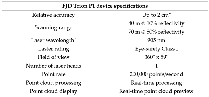 |
Table A2.
Technical specifications of the Xgrids Lixel L2 Pro Lidar Scanner used in this study. Relative accuracy values correspond to manufacturer-reported performance under experimental conditions.
Table A2.
Technical specifications of the Xgrids Lixel L2 Pro Lidar Scanner used in this study. Relative accuracy values correspond to manufacturer-reported performance under experimental conditions.
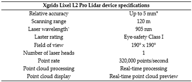 |
Table A3.
FJD Trion Model and cloud compare forestry processing parameters and approximate times for HMLS datasets. Specifically, forestry parameter extractions: tree segmentation, diameter at breast height (DBH) calculation, and crown area deviation; Settings for point cloud cleaning in Cloud Compare: SQR filter and Noise Filter; FJD Trion Model settings for individual quadrat pasture vegetation data extraction in FJD Model Trion: clipping box, and grids volume.
Table A3.
FJD Trion Model and cloud compare forestry processing parameters and approximate times for HMLS datasets. Specifically, forestry parameter extractions: tree segmentation, diameter at breast height (DBH) calculation, and crown area deviation; Settings for point cloud cleaning in Cloud Compare: SQR filter and Noise Filter; FJD Trion Model settings for individual quadrat pasture vegetation data extraction in FJD Model Trion: clipping box, and grids volume.
| FJD Trion Model - point cloud mapping | Rangelands forest | Grassland | Mangrove forest | Wetland forest |
|---|---|---|---|---|
| Device model | P1 | P1 | P1 | P1 |
| Scan scene | Outdoor | Outdoor | Outdoor | Outdoor |
| Mapping range (m) | 1.00m – 90.00m | 1.00m – 90.00m | 1.00m – 90.00m | 1.00m – 90.00m |
| RTK fusion | On | On | On | On |
| Optimise with control point | Off | Off | Off | Off |
| Point cloud colourisation | On | On | On | On |
| Back to starting point | Enable | Enable | Enable | Enable |
| Moving object removal | Enable | Enable | Enable | Enable |
| Image filtering | Enable | Enable | Enable | Enable |
| RTK receiver offsets (deviation x, y, z) | 0, 0, 0 | 0, 0, 0 | 0, 0, 0 | 0, 0, 0 |
| Colouring range | 15m | 15m | 15m | 15m |
| Colouring frequency | Low | Low | Low | Low |
| Object removal | Motion blur optimisation | Motion blur optimisation | Motion blur optimisation | Motion blur optimisation |
| Time (h) | 5 | 3 | 4 | 5 |
| FJD Trion Model - coordinate transform | ||||
| Transform type | Unknown matrix | Unknown matrix | Unknown matrix | Unknown matrix |
| Point order correction | Enable | Enable | Enable | Enable |
| Alignment point | Click | Click | Click | Click |
| Time (h) | 3 | 2 | 2 | 3 |
| Cloud Compare cleaning – SQR filter | ||||
| No. points for mean distance estimation | 6 | 6 | 6 | 6 |
| Standard deviation multiplier threshold (sigma) | 1.00 | 1.00 | 1.00 | 1.00 |
| Time (h) | 0.05 | 0.05 | 0.05 | 0.05 |
| Cloud Compare cleaning - noise filter | ||||
| Neighbours | Radius (sphere) | Radius (sphere) | Radius (sphere) | Radius (sphere) |
| Max errors | Relative (1.0) | Relative (1.0) | Relative (1.0) | Relative (1.0) |
| Time (h) | 0.05 | 0.05 | 0.05 | 0.05 |
| FJD Trion Model - ground point extraction | ||||
| Grid Size (m) | 0.5 | N/A | 0.5 | 0.5 |
| Ground Thickness (m) | 0.5 | N/A | 0.5 | 0.5 |
| Density Sampling Parameters | 2.0 | N/A | 2.0 | 2.0 |
| Time (h) | 0.1 | N/A | 0.1 | 0.1 |
| FJD Trion Model - segment by tree | ||||
| Minimum number of points (pts) | 5000 | N/A | 2000 | 5000 |
| Minimum Grid Edge Length | 0.10 | N/A | 0.10 | 0.10 |
| Time (h) | 0.2 | N/A | 0.2 | 0.2 |
| FJD Trion Model - crown analysis | ||||
| Accuracy | High | High | High | High |
| Time (h) | 0 | 0 | 0 | 0 |
| FJD Trion Model - property Calculation | ||||
| Breast Location (m) | 1.5 | N/A | 1.5 | 1.5 |
| Ground Diameter Location (m) | 0.1 | N/A | 0.1 | 0.1 |
| Min. DBH (m) | 0.1 | N/A | 0.1 | 0.1 |
| Max. DBH (m) | 10 | N/A | 10 | 10 |
| Crown Width | On | N/A | On | On |
| Crown Volume | On | N/A | On | On |
| Crown Projection Area | On | N/A | On | On |
| Stem Length | On | N/A | On | On |
| Time (h) | 0.05 | N/A | 0.05 | 0.05 |
| FJD Trion Model - grids volume | ||||
| Define Reference Plane | N/A | z | N/A | N/A |
| Plane Position | N/A | Default | N/A | N/A |
| Calculation Method | N/A | Interpolate | N/A | N/A |
| Step | N/A | 0.001, 0.1 | N/A | N/A |
| Cell Height | N/A | Maximum height | N/A | N/A |
| Time (h) | N/A | 5 | N/A | N/A |
| Total processing time (h) | 8.45 | 10.1 | 6.45 | 8.45 |
10 Due to the use of various tools across multiple computers, accurately measuring individual processing times is challenging. The recorded times reflect only the duration of each process, and not include time spent problem solving, and thus times should be considered as approximate values.
Table A4.
Metashape processing parameters and settings tools used in creating point clouds for UAV SfM-MVS data.
Table A4.
Metashape processing parameters and settings tools used in creating point clouds for UAV SfM-MVS data.
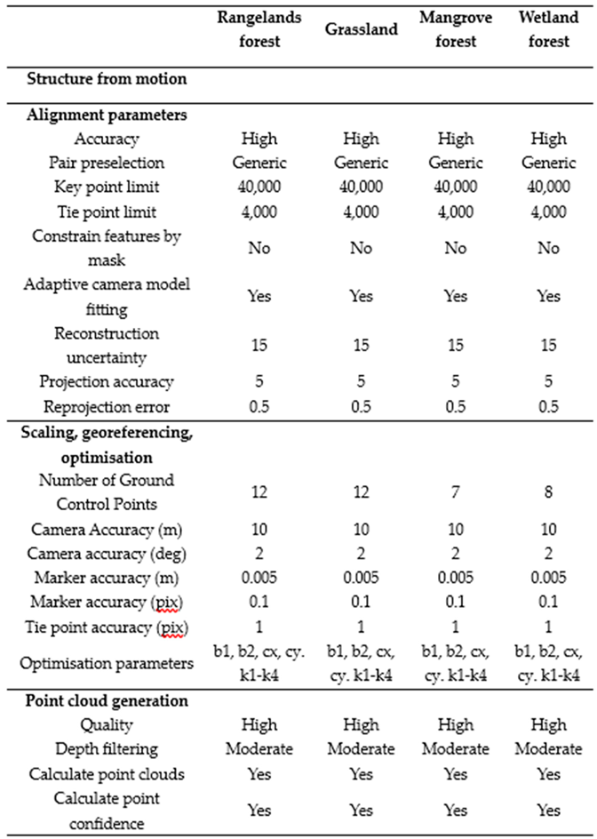 |
Table A5.
Summary of approximate hardware and software costs for HMLS and UAV SfM-MVS systems used in this study, and their respective outcome averages for: processing times, georeferenced position error, DBH and tussock height estimation error.
Table A5.
Summary of approximate hardware and software costs for HMLS and UAV SfM-MVS systems used in this study, and their respective outcome averages for: processing times, georeferenced position error, DBH and tussock height estimation error.
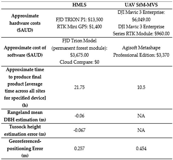 |
Table A6.
LiDAR Virtual Machine hardware specifications used to process all HMLS datasets in this study.
Table A6.
LiDAR Virtual Machine hardware specifications used to process all HMLS datasets in this study.
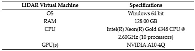 |
Table A7.
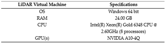
Metashape Virtual Machine hardware specifications used to process all UAV SfM-MVS datasets in this study.
Table A7.
Metashape Virtual Machine hardware specifications used to process all UAV SfM-MVS datasets in this study.
 |
References
- Chambers, J.; et al. Research Priorities for Tropical Ecosystems Under Climate Change:: Workshop Report; Office of Biological and Environmental Research, 2012. [Google Scholar]
- Cuenca-Ocay, G. Mangrove ecosystems’ role in climate change mitigation. Davao Res. J. 2019, 12(2), 72–75. [Google Scholar] [CrossRef]
- Melati, D. MANGROVE ECOSYSTEM AND CLIMATE CHANGE MITIGATION: A LITERATURE REVIEW. J. Sains Dan Teknol. Mitigasi Bencana 2021, 16, 1–8. [Google Scholar] [CrossRef]
- Mubaraq, A.; et al. Carbon and Nitrogen Management in Mangrove Ecosystems in Reducing Greenhouse Gas Emissions: Ecological and Islamic Perspective; 2024. [Google Scholar]
- Zedler, J.B.; Kercher, S.M. Wetland resources: Status, trends, ecosystem services, and restorability. Annu. Rev. Environ. Resour. 2005, 30, 39–74. [Google Scholar] [CrossRef]
- Davidson, N.C.; et al. Worth of wetlands: revised global monetary values of coastal and inland wetland ecosystem services. Marine and Freshwater Research 2019. [Google Scholar] [CrossRef]
- Spangler, L.; et al. Rangeland sequestration potential assessment; Montana State Univ.: Bozeman, MT (United States), 2012. [Google Scholar]
- Tennigkeit, T.; Wilkes, A. An assessment of the potential for carbon finance in rangelands. 2008. [Google Scholar] [CrossRef]
- Bailey, R.G. Ecosystem geography: from ecoregions to sites; Springer Science & Business Media, 2009. [Google Scholar]
- Boval, M.; Dixon, R. The importance of grasslands for animal production and other functions: a review on management and methodological progress in the tropics. Anim. An. Int. J. Anim. Biosci. 2012. 6 5, 748–62. [Google Scholar] [CrossRef]
- Brown, J.R.; Thorpe, J. Climate Change and Rangelands: Responding Rationally to Uncertainty; 2008. [Google Scholar]
- Boone, R.B.; et al. Climate change impacts on selected global rangeland ecosystem services. Glob. Change Biol. 2018, 24, 1382–1393. [Google Scholar]
- Mohd Zaki, N.A.; Abd Latif, Z. Carbon sinks and tropical forest biomass estimation: a review on role of remote sensing in aboveground-biomass modelling. Geocarto Int. 2017, 32, 701–716. [Google Scholar]
- Fidelis, A.; Lyra, M.S.; Pivello, V.R. Above- and below-ground biomass and carbon dynamics in Brazilian Cerrado wet grasslands. J. Veg. Sci. 2013, 24, 356–364. [Google Scholar] [CrossRef]
- Twilley, R.R.; Chen, R.H.; Hargis, T. Carbon sinks in mangroves and their implications to carbon budget of tropical coastal ecosystems. Water, Air, and Soil Pollution 1992, 64, 265–288. [Google Scholar] [CrossRef]
- Pugh, T.A.; et al. Important role of forest disturbances in the global biomass turnover and carbon sinks. Nat. Geosci. 2019, 12(9), 730–735. [Google Scholar] [CrossRef] [PubMed]
- Myneni, R.B.; et al. A large carbon sink in the woody biomass of Northern forests. Proc. Natl. Acad. Sci. 2001, 98(26), 14784–14789. [Google Scholar] [CrossRef] [PubMed]
- Yu, Y. Global Distribution of Carbon Stock in Live Woody Vegetation; 2013. [Google Scholar]
- Friess, D.A.; et al. Blue carbon science, management and policy across a tropical urban landscape. Landsc. Urban Plan. 2023, 230, 104610. [Google Scholar] [CrossRef]
- Pham, T.D.; et al. Remote Sensing Approaches for Monitoring Mangrove Species, Structure, and Biomass: Opportunities and Challenges. Remote Sens. 2019, 11. [Google Scholar] [CrossRef]
- Suwethaasri, D.; et al. A critical review of exploring the recent trends and technological advancements in forest biomass estimation. Plant Sci. Today 2025. [Google Scholar] [CrossRef]
- Denboba, M.A. Grazing management and carbon sequestration in the Dry Lowland Rangelands of Southern Ethiopia. Sustain. Environ. 2022, 8(1), 2046959. [Google Scholar] [CrossRef]
- Pasut, C.; et al. Aboveground biomass relationship with canopy cover and vegetation to improve carbon change monitoring in rangelands. Ecosphere 2025, 16(4), e70231. [Google Scholar] [CrossRef]
- Lu, D. The potential and challenge of remote sensing-based biomass estimation. Int. J. Remote Sens. 2006, 27(7), 1297–1328. [Google Scholar] [CrossRef]
- Krause, P.; et al. Using terrestrial laser scanning to evaluate non-destructive aboveground biomass allometries in diverse Northern California forests. In Frontiers in Remote Sensing; 2023. [Google Scholar]
- Fan, G.; et al. AdQSM: A New Method for Estimating Above-Ground Biomass from TLS Point Clouds. Remote Sens. 2020, 12, 3089. [Google Scholar] [CrossRef]
- Toraño Caicoya, A.; et al. Forest Above-Ground Biomass Estimation From Vertical Reflectivity Profiles at L-Band. IEEE Geosci. Remote Sens. Lett. 2015, 12, 1–5. [Google Scholar] [CrossRef]
- Lu, D.; et al. A survey of remote sensing-based aboveground biomass estimation methods in forest ecosystems. Int. J. Digit. Earth 2016, 9(1), 63–105. [Google Scholar]
- Kumar, L.; et al. Review of the use of remote sensing for biomass estimation to support renewable energy generation. J. Appl. Remote Sens. 2015, 9, 097696. [Google Scholar] [CrossRef]
- Gonçalves, J.A.; et al. Three-dimensional data collection for coastal management – efficiency and applicability of terrestrial and airborne methods. Int. J. Remote Sens. 2018, 39(24), 9380–9399. [Google Scholar] [CrossRef]
- Kuyah, S.; Rosenstock, T.S. Optimal measurement strategies for aboveground tree biomass in agricultural landscapes. Agrofor. Syst. 2015, 89(1), 125–133. [Google Scholar]
- Gard, S.; Neal, M.; Minnee, E. Pasture performance tools: current and future state. J. N. Z. Grassl. 2024, 273–279. [Google Scholar] [CrossRef]
- Kallenbach, R.L. Describing the dynamic: Measuring and assessing the value of plants in the pasture. Crop Sci. 2015, 55(6), 2531–2539. [Google Scholar] [CrossRef]
- HAO, Q.; HUANG, C. A review of forest aboveground biomass estimation based on remote sensing data. Chin. J. Plant Ecol. 2023, 47(10), 1356. [Google Scholar] [CrossRef]
- Goetz, S.J.; et al. Mapping and monitoring carbon stocks with satellite observations: a comparison of methods. Carbon Balance Manag. 2009, 4(1), 2. [Google Scholar] [CrossRef] [PubMed]
- Anderson, G.; Rawlings, M.; Ogle, G. Mitigation of saturation in satellite pasture measurement via incorporation of a statistical pasture growth model. J. N. Z. Grassl. 2020, 191–198. [Google Scholar] [CrossRef]
- Quinones, M.J.; Hoekman, D.H. Exploration of factors limiting biomass estimation by polarimetric radar in tropical forests. IEEE Trans. Geosci. Remote Sens. 2004, 42, 86–104. [Google Scholar] [CrossRef]
- Baccini, A.; et al. Reply to Comment on ‘A first map of tropical Africa’s above-ground biomass derived fromsatellite imagery’. Environ. Res. Lett. 2011, 6(4), 049002. [Google Scholar] [CrossRef]
- He, Q.; et al. Above-Ground Biomass and Biomass Components Estimation Using LiDAR Data in a Coniferous Forest. Forests 2013, 4(4), 984–1002. [Google Scholar] [CrossRef]
- Ma, J.; et al. Total and component forest aboveground biomass inversion via LiDAR-derived features and machine learning algorithms. In Frontiers in Plant Science; 2023; pp. 14–2023. [Google Scholar]
- Georgopoulos, N.; et al. Estimation of Individual Tree Stem Biomass in an Uneven-Aged Structured Coniferous Forest Using Multispectral LiDAR Data. Remote Sens. 2021, 13(23), 4827. [Google Scholar] [CrossRef]
- Lu, D.; et al. Aboveground forest biomass estimation with Landsat and LiDAR data and uncertainty analysis of the estimates. Int. J. For. Res. 2012, 2012(1), 436537. [Google Scholar] [CrossRef]
- Lu, D.; et al. A survey of remote sensing-based aboveground biomass estimation methods in forest ecosystems. Int. J. Digit. Earth 2016, 9(1), 63–105. [Google Scholar]
- Pereira Mendes, C.; Lim, N.T.-L. EcoLiDAR: An economical LiDAR scanner for ecological research. PLoS ONE 2024, 19(6), e0298712. [Google Scholar] [CrossRef] [PubMed]
- Hill, T.C.; et al. Are inventory based and remotely sensed above-ground biomass estimates consistent? PLoS ONE 2013, 8(9), e74170. [Google Scholar] [CrossRef] [PubMed]
- Fowler, A.; Kadatskiy, V. Accuracy and error assessment of terrestrial, mobile and airborne lidar. Proceedings of American Society of Photogrammetry and Remote Sensing Conference (ASPRP 2011), 2011. [Google Scholar]
- Jurado, D.; et al. Portable LiDAR Scanners: Precision Mapping at Your Fingertips. 2024; pp. 1–3. [Google Scholar]
- Vogt, J.; Ilic, M.; Bogenberger, K. A mobile mapping solution for VRU Infrastructure monitoring via low-cost LiDAR-sensors. J. Locat. Based Serv. 2023, 17, 1–23. [Google Scholar] [CrossRef]
- Zeybek, M. Indoor mapping and positioning applications of hand-held LiDAR Simultaneous localization and mapping (SLAM) systems. Turk. Lidar J. 2021. [Google Scholar] [CrossRef]
- Sepasgozar, S.; Lim, S.; Shirowzhan, S. Implementation of Rapid As-built Building Information Modeling Using Mobile LiDAR. 2014, 2014. [Google Scholar]
- Westling, F.; et al. Applications of LiDAR for Productivity Improvement on Construction Projects: Case Studies from Active Sites; 2020. [Google Scholar]
- Chase, A.F.; et al. Geospatial revolution and remote sensing LiDAR in Mesoamerican archaeology. Proc. Natl. Acad. Sci. 2012, 109(32), 12916–12921. [Google Scholar] [CrossRef] [PubMed]
- Vinci, G.; et al. LiDAR Applications in Archaeology: A Systematic Review. Archaeol. Prospect. 2024, 1–21. [Google Scholar]
- Rodríguez-Gonzálvez, P.; et al. Mobile LiDAR System: New Possibilities for the Documentation and Dissemination of Large Cultural Heritage Sites. Remote Sens. 2017, 9, 189. [Google Scholar] [CrossRef]
- Gallagher, J.; Josephs, R. Using LiDAR to Detect Cultural Resources in a Forested Environment: an Example from Isle Royale National Park, Michigan, USA. Archaeol. Prospect. 2008, 15, 187–206. [Google Scholar] [CrossRef]
- Proudman, A.; et al. Towards real-time forest inventory using handheld LiDAR. Robot. Auton. Syst. 2022, 157, 104240. [Google Scholar] [CrossRef]
- de Nobel, J.S.; et al. Towards Prediction and Mapping of Grassland Aboveground Biomass Using Handheld LiDAR. Remote Sens. 2023, 15, 1754. [Google Scholar] [CrossRef]
- Marshall, A.; et al. Handheld lidar as a tool for characterizing wood-rich river corridors. River Res. Appl. 2024, 40. [Google Scholar]
- Zeybek, M.; Vatandaşlar, C. An Automated Approach for Extracting Forest Inventory Data from Individual Trees Using a Handheld Mobile Laser Scanner. Croat. J. For. Eng. 2021, 42. [Google Scholar]
- Department of Climate Change, E. the Environment and Water, Einasleigh Uplands bioregion; Canberra, ACT, 2008. [Google Scholar]
- Neldner, V.J.N.; Wilson, Rosemary E.; McDonald, Bruce A.; Ford, Wendy J. F.; Accad, Andrew J.; Albert. The Vegetation of Queensland: Descriptions of Broad Vegetation Groups; 2023. [Google Scholar]
- WillyWeather. Mingela Rain Statitics. 2025 23/12/2025. Available online: https://rainfall.willyweather.com.au/qld/northern/mingela.html.
- Department of Climate Change, E. the Environment and Water, Mitchell Grass Downs bioregion. 2008. [Google Scholar] [CrossRef] [PubMed]
- Bureau of Meterology. Summary statisitcs Richmond Post Office. 2025 23/12/2025. Available online: https://www.bom.gov.au/climate/averages/tables/cw_030045.shtml.
- Gardens, M.R.B. Central Queensland Coast Bioregion Review. n.d. Available online: https://www.mackayregionalbotanicgardens.com.au/Education/review/central_queensland_coast_bioregion.
- Walham, N.G.A.; Jarihani, B. Cape Palmerston modelling tidal water ingress and vegetation survey; Centre for Tropical Water & Aquatic Ecosystem Research (TropWATER), James Cook University: Townsville, Australia, 2025; p. 56. [Google Scholar]
- WillyWeather. Cape Palmeston Rainfall Statistics. 2025 23/12/2025. Available online: https://rainfall.willyweather.com.au/qld/mackay/cape-palmerston.html.
- Science, D.o.E.a., Cape Palmerston National Park Managment Plan. 2013.
- de Nobel, J.S.; et al. Towards Prediction and Mapping of Grassland Aboveground Biomass Using Handheld LiDAR. Remote Sens. 2023, 15(7), 1754. [Google Scholar] [CrossRef]
- Kükenbrink, D.; et al. Evaluating the potential of handheld mobile laser scanning for an operational inclusion in a national forest inventory – A Swiss case study. Remote Sens. Environ. 2025, 321, 114685. [Google Scholar] [CrossRef]
- Safari, H.; et al. Comparing mobile and static assessment of biomass in heterogeneous grassland with a multi-sensor system. J. Sens. Sens. Syst. 2016, 5, 301–312. [Google Scholar] [CrossRef]
- Sofia, S.; et al. View of Comparing efficiency, timing and costs of different walking paths in HMLS LIDAR survey. Ann. For. Res. 2024, 67, 87–107. [Google Scholar] [CrossRef]
- Chudá, J.; et al. Prompt Mapping Tree Positions with Handheld Mobile Scanners Based on SLAM Technology. Land 2024, 13, 93. [Google Scholar] [CrossRef]
- Ferrara, C.; et al. Mapping Understory Vegetation Density in Mediterranean Forests: Insights from Airborne and Terrestrial Laser Scanning Integration. Sensors 2023, 23, 511. [Google Scholar] [CrossRef] [PubMed]
- Lin, Y.; et al. Validation of Mobile Laser Scanning for Understory Tree Characterization in Urban Forest. Sel. Top. Appl. Earth Obs. Remote Sens. IEEE J. 2014, 7, 3167–3173. [Google Scholar] [CrossRef]
- Hamraz, H.; Contreras, M.; Zhang, J. Forest understory trees can be segmented accurately within sufficiently dense airborne laser scanning point clouds. Scientific Reports, 2017, 7.
- Donager, J.J.; Sánchez Meador, A.J.; Blackburn, R.C. Adjudicating Perspectives on Forest Structure: How Do Airborne, Terrestrial, and Mobile Lidar-Derived Estimates Compare? Remote Sens. 2021, 13, 2297. [Google Scholar] [CrossRef]
- Paijitprapaporn, C.; Thongtan, T.; Satirapod, C. Accuracy assessment of integrated GNSS measurements with LIDAR mobile mapping data in urban environments. Meas. Sens. 2021, 18, 100078. [Google Scholar] [CrossRef]
- Famiglietti, N.A.; et al. A Test on the Potential of a Low Cost Unmanned Aerial Vehicle RTK/PPK Solution for Precision Positioning. Sensors 2021, 21, 3882. [Google Scholar] [CrossRef] [PubMed]
- Jones, C.E.; et al. Use of Mobile Laser Scanning (MLS) to Monitor Vegetation Recovery on Linear Disturbances. Forests 2022, 13, 1743. [Google Scholar] [CrossRef]
- Qi, Y.; et al. Comparing tree attributes derived from quantitative structure models based on drone and mobile laser scanning point clouds across varying canopy cover conditions. ISPRS J. Photogramm. Remote Sens. 2022, 192, 49–65. [Google Scholar] [CrossRef]
- Coveney, S.; Fotheringham, A. Terrestrial laser scan error in the presence of dense ground vegetation. Photogramm. Rec. 2011, 26, 307–324. [Google Scholar] [CrossRef]
- Watt, M.S.; et al. Use of a Consumer-Grade UAV Laser Scanner to Identify Trees and Estimate Key Tree Attributes across a Point Density Range. Forests 2024, 15, 899. [Google Scholar] [CrossRef]
- Xiangbing, C.; et al. Correcting drifting error of mobile laser scanner using model-based loop closure detection. Proc.SPIE., 2024. [Google Scholar]
- Anand, B.; et al. Comparative Run Time Analysis of LiDAR Point Cloud Processing with GPU and CPU. 2020, 650–654. [Google Scholar] [CrossRef]
- Muñoz, F.; et al. CPU and GPU oriented optimizations for LiDAR data processing. J. Comput. Sci. 2024, 79, 102317. [Google Scholar] [CrossRef]
- Venugopalan, V.; Kannan, S. Accelerating real-time LiDAR data processing using GPUs. 2013, 1168–1171. [Google Scholar]
Figure 1.
(a) Map showing the broader region of the rangelands forest. Background map is a UAV ortho-photo mosaic of the region. (b) Close up of UAV ortho-photo mosaic of the specific site. (c) Ground image of the typical rangelands forest vegetation for the study site. This included different vegetation and grass, varying topography, and the presence of gully erosion. This site was selected to represent low vegetation complexity.
Figure 1.
(a) Map showing the broader region of the rangelands forest. Background map is a UAV ortho-photo mosaic of the region. (b) Close up of UAV ortho-photo mosaic of the specific site. (c) Ground image of the typical rangelands forest vegetation for the study site. This included different vegetation and grass, varying topography, and the presence of gully erosion. This site was selected to represent low vegetation complexity.
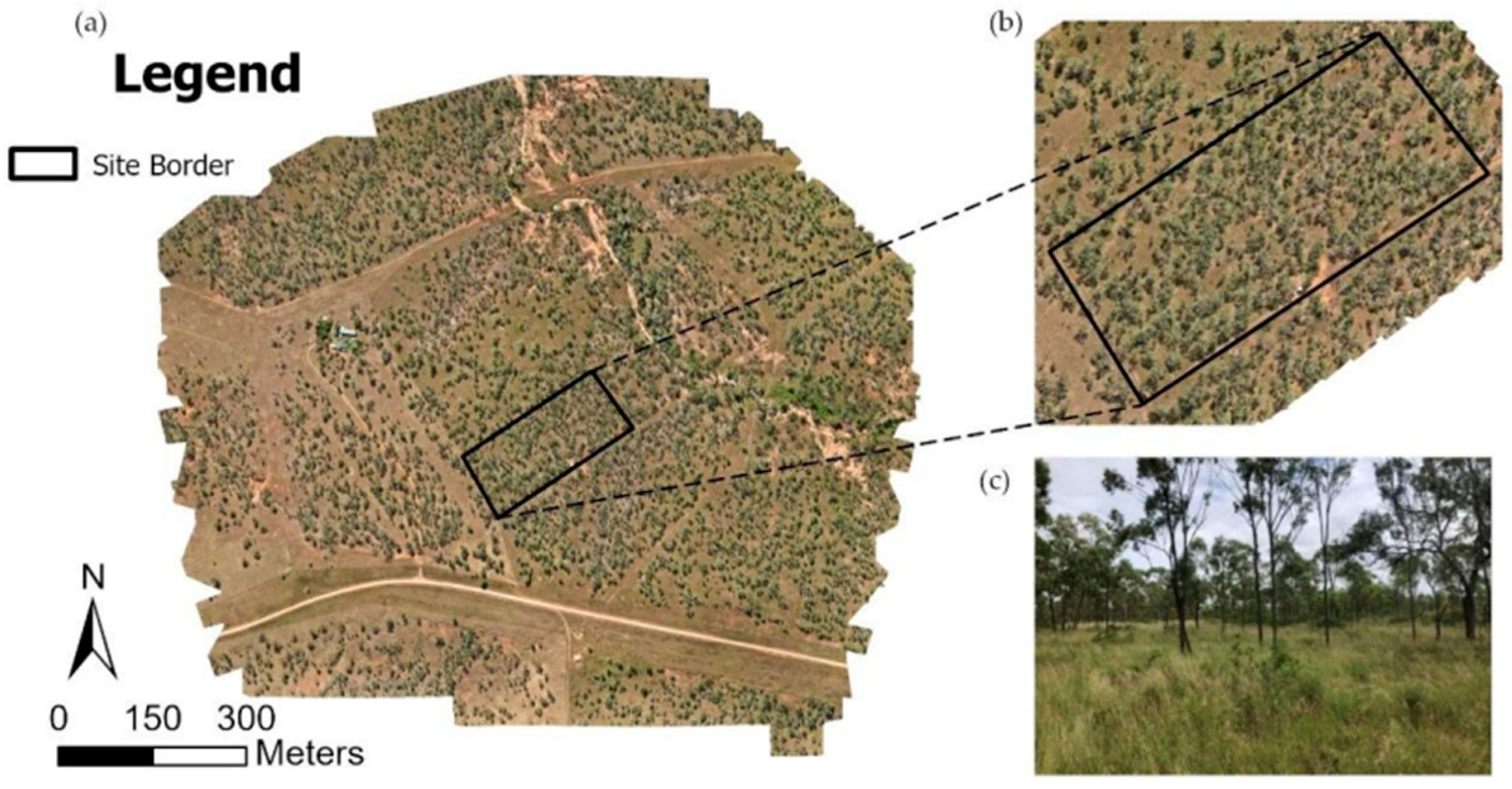
Figure 2.
(a) Map showing the broader region of the grasslands site. Background map is a UAV ortho-photo mosaic of the region. (b) Close up of UAV ortho-photo mosaic of the specific site. (c) Ground image of the typical grasslands vegetation for the study site. This site was selected to represent moderate vegetation complexity.
Figure 2.
(a) Map showing the broader region of the grasslands site. Background map is a UAV ortho-photo mosaic of the region. (b) Close up of UAV ortho-photo mosaic of the specific site. (c) Ground image of the typical grasslands vegetation for the study site. This site was selected to represent moderate vegetation complexity.
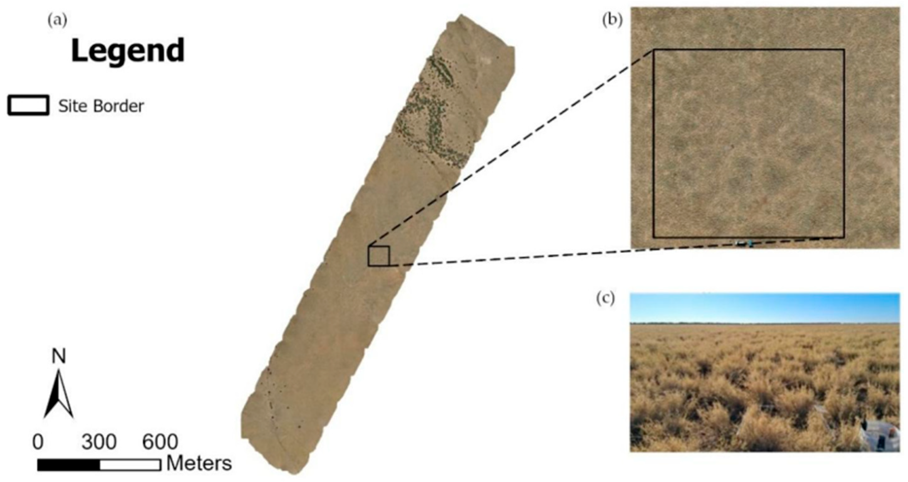
Figure 3.
(a) Map showing the broader region of the mangrove at Cape Palmerston. Background map is a UAV ortho-photo mosaic of Cape Palmerston. (b) Close up of UAV ortho-photo mosaic of the specific mangrove forest study site. (c) Ground image of the mangrove vegetation for the study site. This site is selected to represent high vegetation complexity.
Figure 3.
(a) Map showing the broader region of the mangrove at Cape Palmerston. Background map is a UAV ortho-photo mosaic of Cape Palmerston. (b) Close up of UAV ortho-photo mosaic of the specific mangrove forest study site. (c) Ground image of the mangrove vegetation for the study site. This site is selected to represent high vegetation complexity.
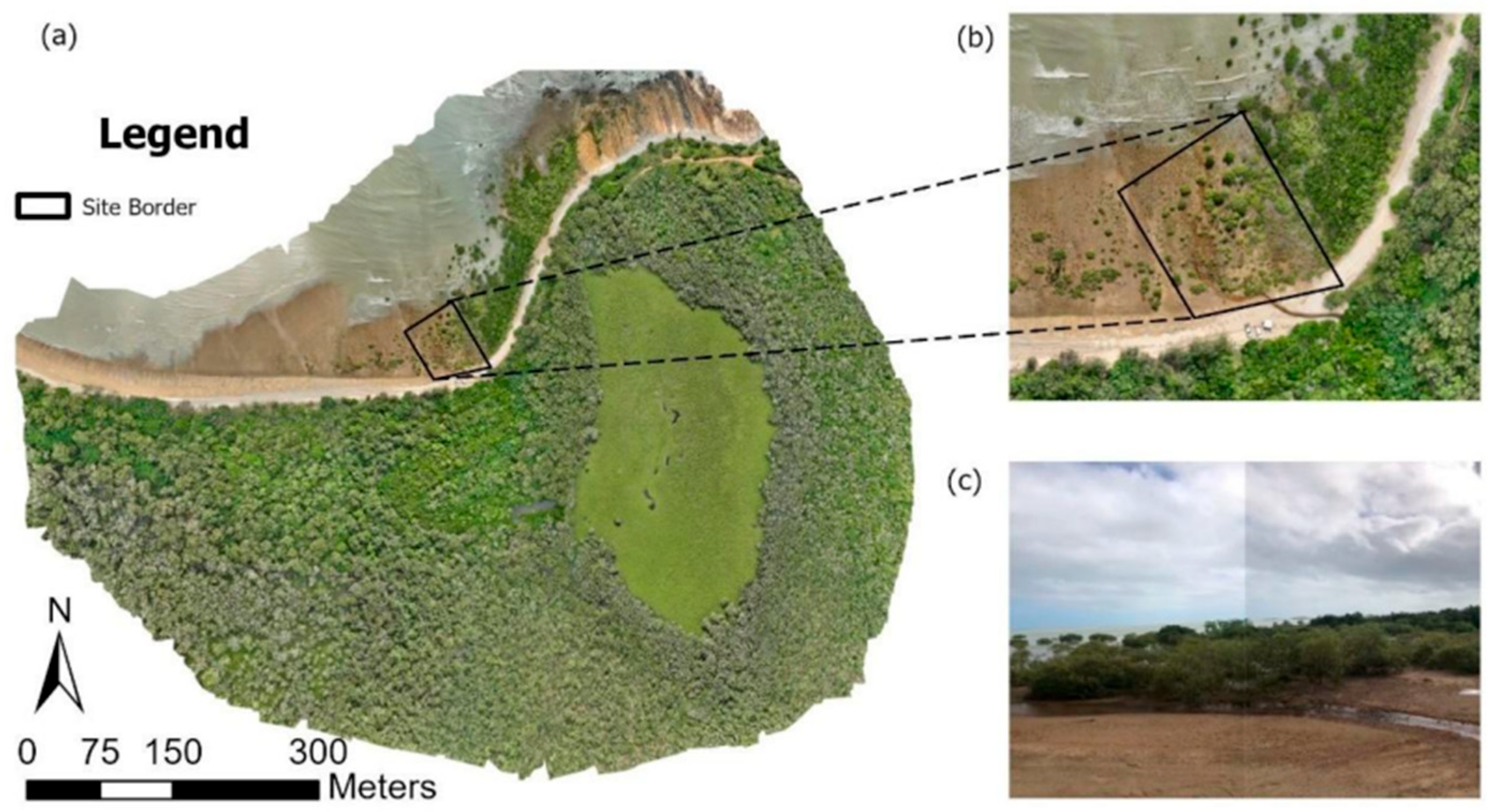
Figure 4.
(a) Map showing the broader region of the estuarine wetland at Cape Palmerston. Background map is a UAV ortho-photo mosaic of Cape Palmerston. (b) Close up of UAV ortho-photo mosaic of the specific study site. (c) Ground image of typical estuarine wetland vegetation for the study site.
Figure 4.
(a) Map showing the broader region of the estuarine wetland at Cape Palmerston. Background map is a UAV ortho-photo mosaic of Cape Palmerston. (b) Close up of UAV ortho-photo mosaic of the specific study site. (c) Ground image of typical estuarine wetland vegetation for the study site.
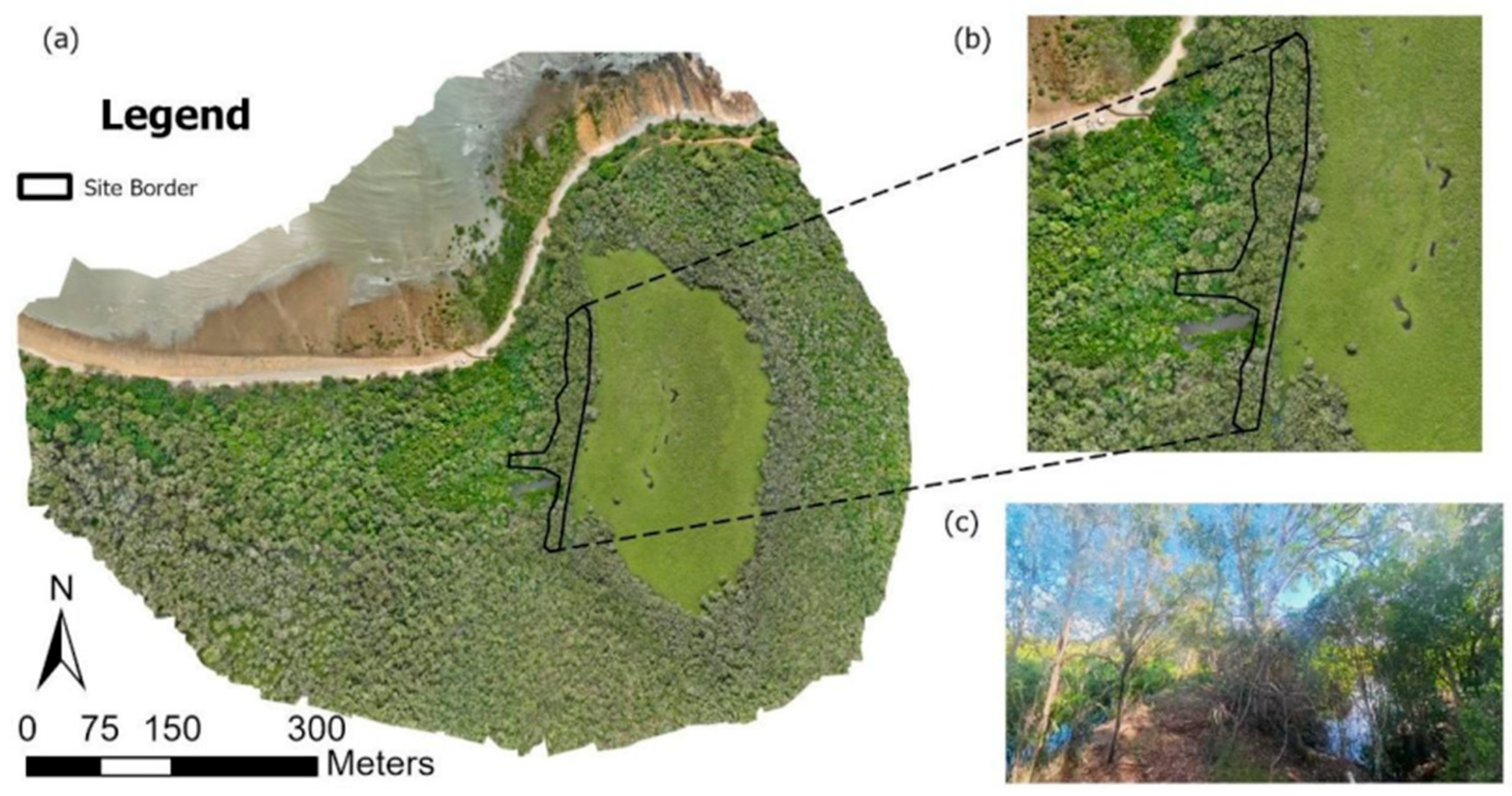
Figure 5.
HMLS looped trajectory survey configuration. Four to eight GCPs were used depending on site size across each site, with one GCP serving as the start/finish position (yellow). Walking trajectories (arrowed lines) followed by randomized looping patterns with site boundary (dashed line), visiting all GCP’s, to mitigate point cloud drift around individual trees.
Figure 5.
HMLS looped trajectory survey configuration. Four to eight GCPs were used depending on site size across each site, with one GCP serving as the start/finish position (yellow). Walking trajectories (arrowed lines) followed by randomized looping patterns with site boundary (dashed line), visiting all GCP’s, to mitigate point cloud drift around individual trees.
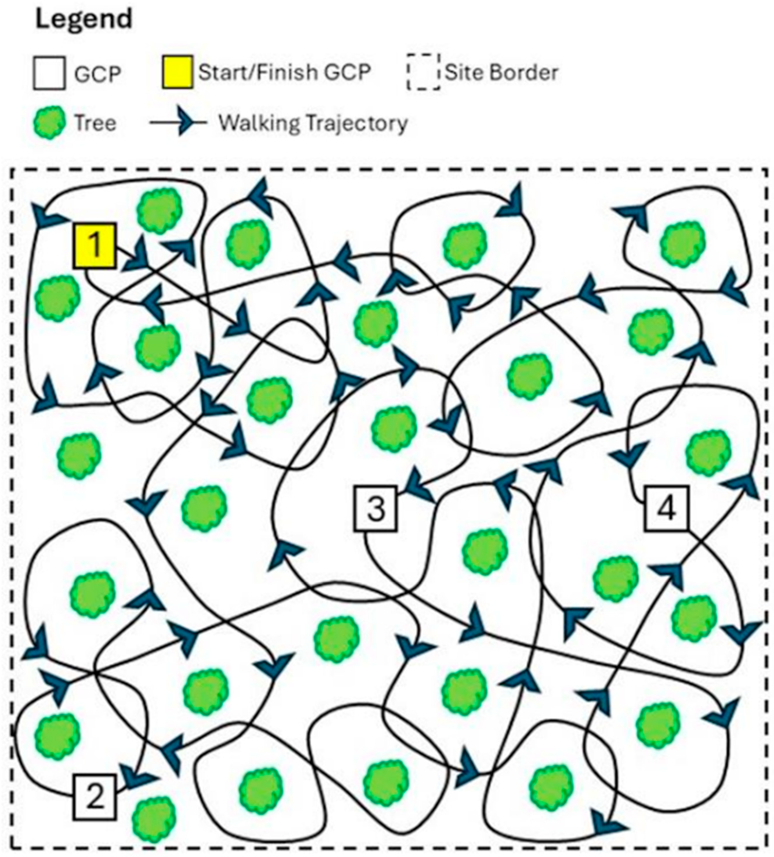
Figure 6.
Site-specific distribution of ground control points (GCPs) used for HMLS and UAV SfM-MVS surveys at the four study sites: (a) grassland; (b) rangeland forest; (c) estuarine wetland forest; and (d) mangrove forest.
Figure 6.
Site-specific distribution of ground control points (GCPs) used for HMLS and UAV SfM-MVS surveys at the four study sites: (a) grassland; (b) rangeland forest; (c) estuarine wetland forest; and (d) mangrove forest.
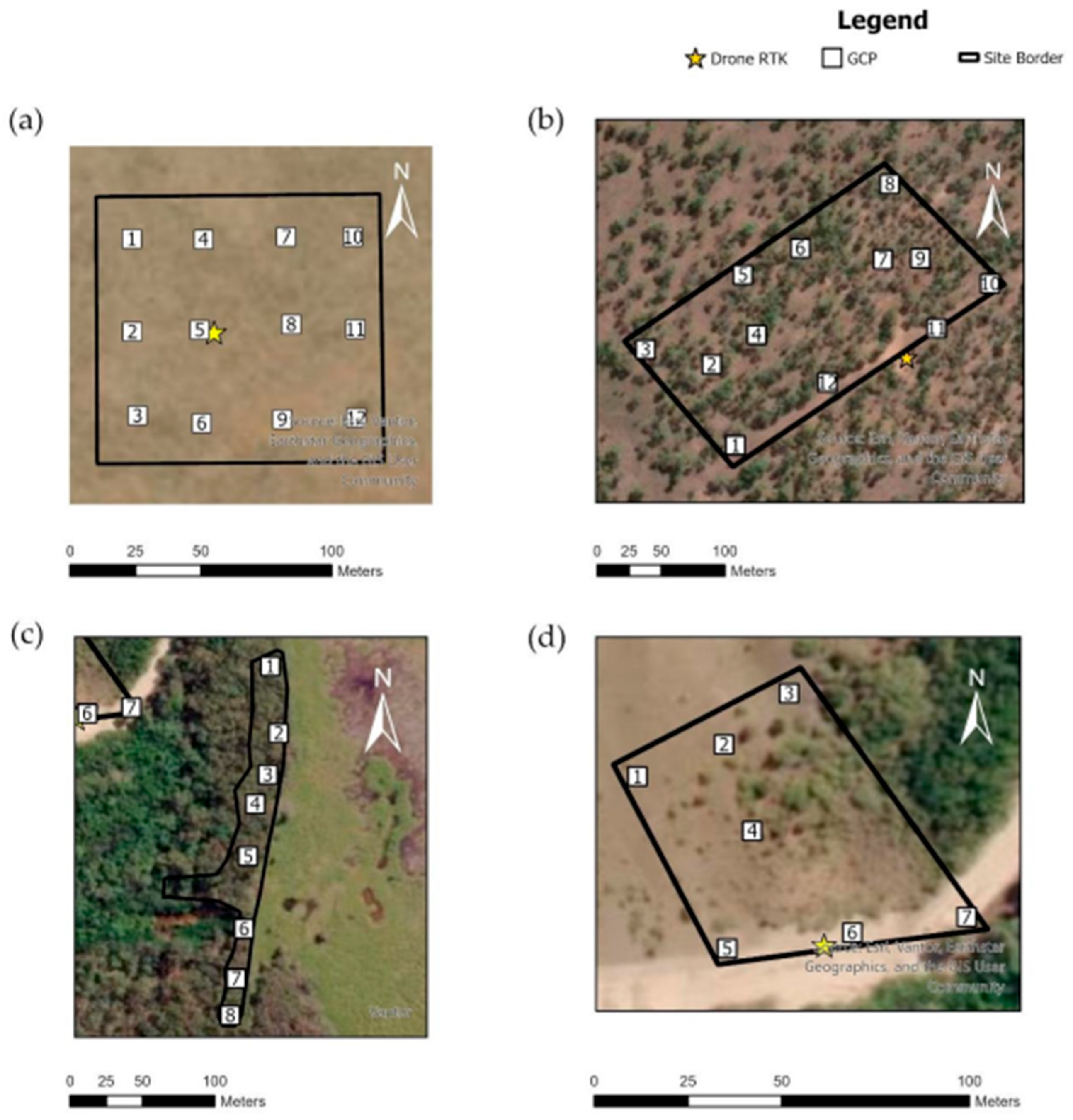
Figure 7.
Layout of the grasslands study site, showing spatial arrangement of 1 x 1 m quadrats used to measure tussock height and weights along three transects within the grassland site.
Figure 7.
Layout of the grasslands study site, showing spatial arrangement of 1 x 1 m quadrats used to measure tussock height and weights along three transects within the grassland site.
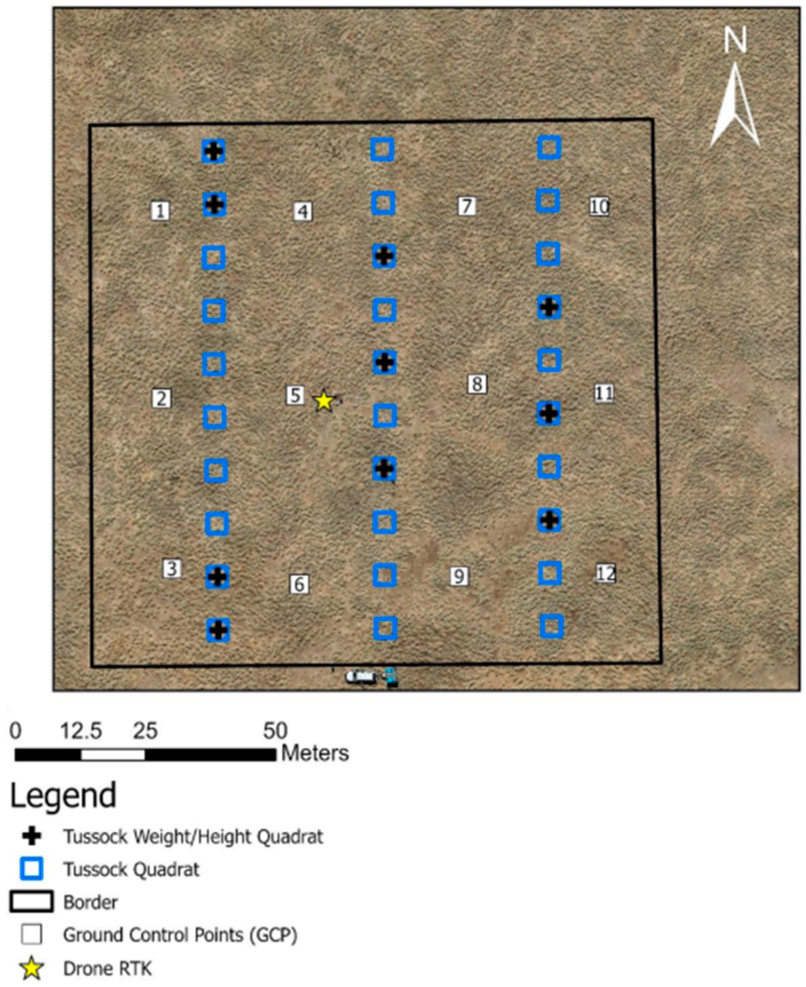
Figure 8.
All HMLS forestry data post-processing workflow, showing (1) point cloud pre-processing; (2) tree model generation; (3) calculation and analysis. (2) Tree model generation is completed by a specialized forestry module designed for automated single-tree segmentation built within FJD Trion Model. (3) Calculation and analysis are completed by automated tree parameter calculation, from identified single trees in FJD Trion Model.
Figure 8.
All HMLS forestry data post-processing workflow, showing (1) point cloud pre-processing; (2) tree model generation; (3) calculation and analysis. (2) Tree model generation is completed by a specialized forestry module designed for automated single-tree segmentation built within FJD Trion Model. (3) Calculation and analysis are completed by automated tree parameter calculation, from identified single trees in FJD Trion Model.
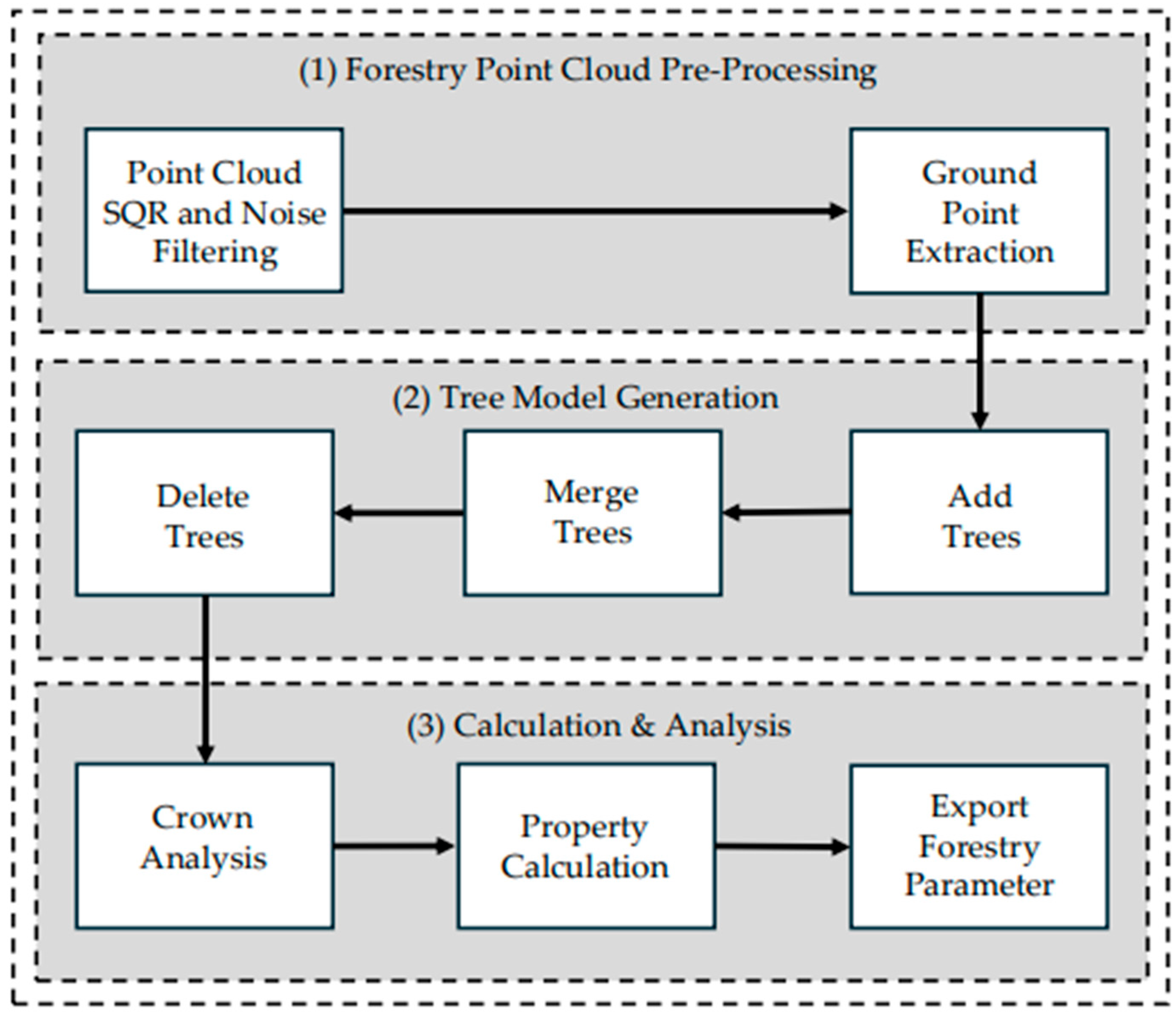
Figure 9.
Angled-down view of colored point clouds produced by FJD Trion P1 system. The left column displays point clouds generated using the HMLS, while the right column shows point clouds derived from the UAV SfM-MVS. Each row represents a different study site: rangelands forest, grasslands, mangrove forest, and estuarine wetland forest. This angled perspective shows three-dimensional structure and vertical complexity of vegetation captured by each method across diverse ecosystems.
Figure 9.
Angled-down view of colored point clouds produced by FJD Trion P1 system. The left column displays point clouds generated using the HMLS, while the right column shows point clouds derived from the UAV SfM-MVS. Each row represents a different study site: rangelands forest, grasslands, mangrove forest, and estuarine wetland forest. This angled perspective shows three-dimensional structure and vertical complexity of vegetation captured by each method across diverse ecosystems.
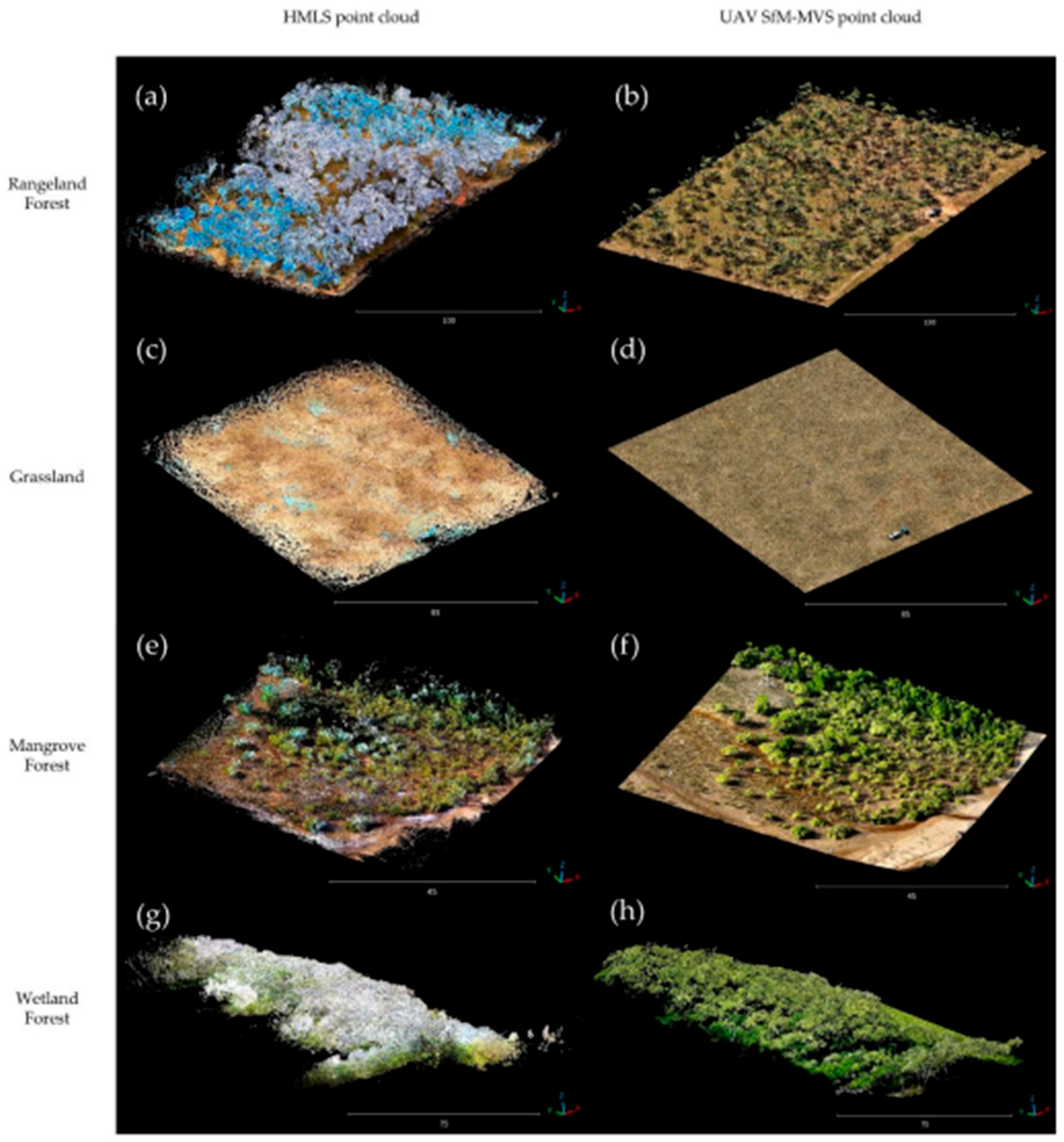
Figure 10.
Top-down view of colored point clouds produced by FJD Trion P1 system. The left column displays point clouds generated using the HMLS, while the right column shows point clouds derived from the UAV SfM-MVS. Each row represents a different study site: rangeland forest, grassland, mangrove forest, and estuarine wetland forest. This perspective shows overall planimetric coverage and general structural characteristics by each method across diverse environments.
Figure 10.
Top-down view of colored point clouds produced by FJD Trion P1 system. The left column displays point clouds generated using the HMLS, while the right column shows point clouds derived from the UAV SfM-MVS. Each row represents a different study site: rangeland forest, grassland, mangrove forest, and estuarine wetland forest. This perspective shows overall planimetric coverage and general structural characteristics by each method across diverse environments.
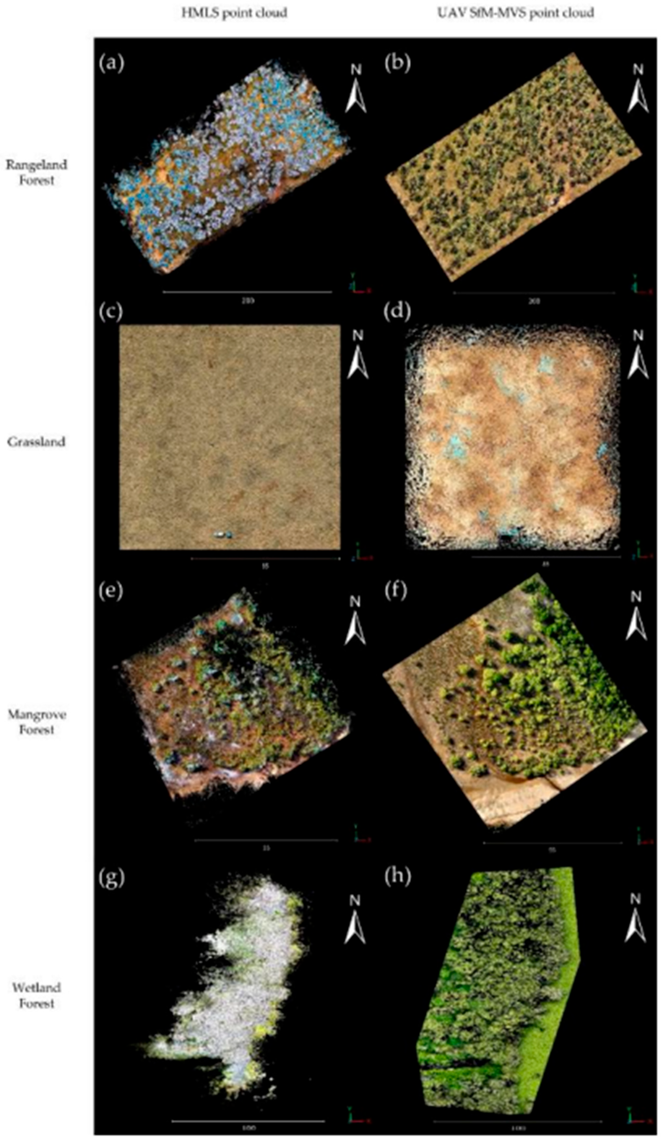
Figure 11.
Comparison of extracted tree entities from HMLS (FJD Trion P1 system) and UAV SFM-MVS point clouds. The left column displays individual tree entities identified from HMLS data, and the right column shows tree entities identified from UAV SfM-MVS data. Each row represents data for a different study site: rangelands forest, mangrove forest, and estuarine wetland forest. Distinct colors represent individual tree entities, while white coloring indicates unclassified points within the respective point clouds, illustrating the efficacy for each method and environment in FJD Trion Model tree segmentation.
Figure 11.
Comparison of extracted tree entities from HMLS (FJD Trion P1 system) and UAV SFM-MVS point clouds. The left column displays individual tree entities identified from HMLS data, and the right column shows tree entities identified from UAV SfM-MVS data. Each row represents data for a different study site: rangelands forest, mangrove forest, and estuarine wetland forest. Distinct colors represent individual tree entities, while white coloring indicates unclassified points within the respective point clouds, illustrating the efficacy for each method and environment in FJD Trion Model tree segmentation.
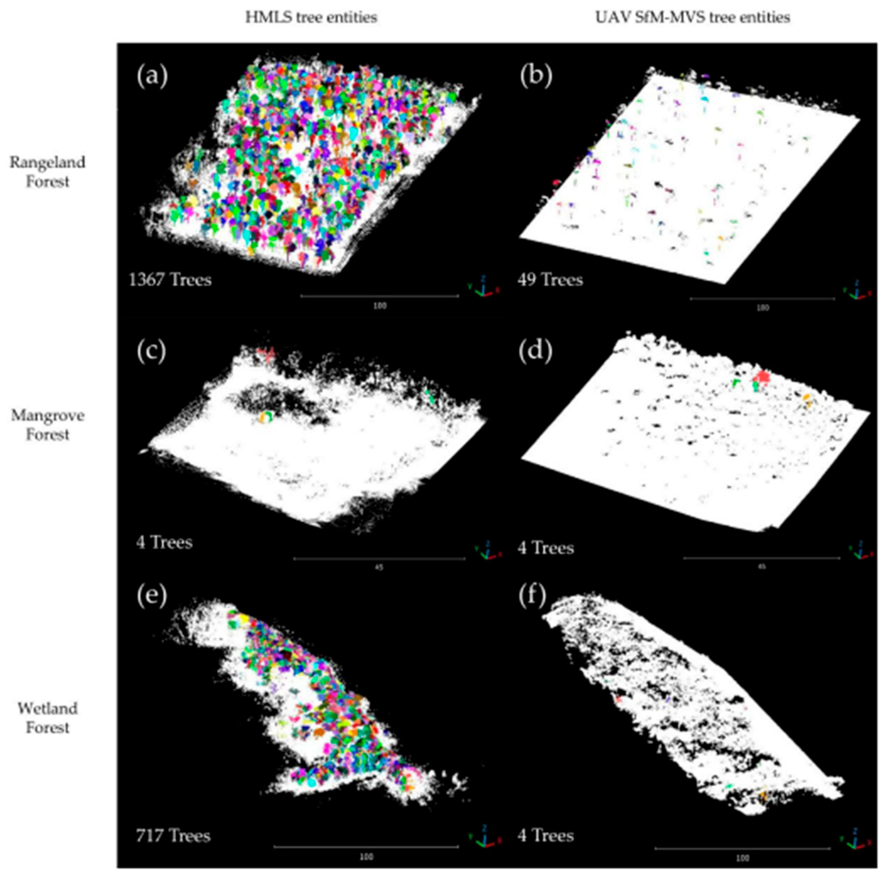
Figure 12.
Example of HMLS-derived (FJD Trion P1) grids volume for a tussock quadrat: (a) raw point cloud; (b) grids volume calculated at 0.001 m3 voxel resolution; (c) grids volume calculated at 0.1m3.
Figure 12.
Example of HMLS-derived (FJD Trion P1) grids volume for a tussock quadrat: (a) raw point cloud; (b) grids volume calculated at 0.001 m3 voxel resolution; (c) grids volume calculated at 0.1m3.
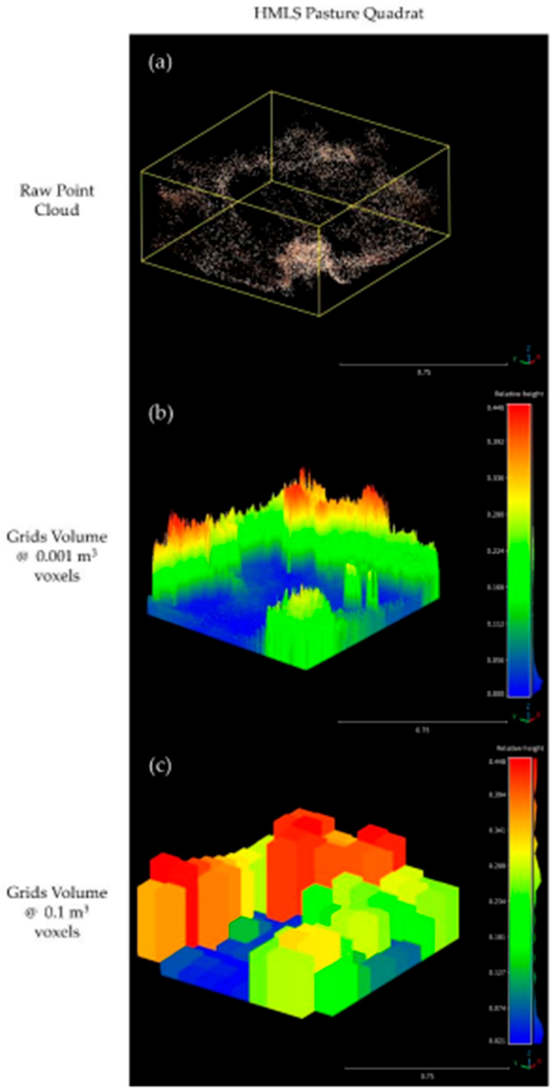
Table 1.
summarises the key characteristics of the four study sites and the primary environmental and operational challenges expected to influence HMLS performance.
Table 1.
summarises the key characteristics of the four study sites and the primary environmental and operational challenges expected to influence HMLS performance.
| Site | Ecosystem | Vegetation Density | Canopy Complexity | Accessibility | Primary Validation Metric |
|---|---|---|---|---|---|
| Grassland | Open tussock grassland | Low | Low | Easy | Height, biomass |
| Rangeland forest | Eucalypt woodland | Moderate | Moderate | Moderate | DBH |
| Mangrove | Mangrove forest | High | High | Difficult | Structural assessment |
| Wetland forest | Estuarine wetland forest | Very high | Very high | Difficult | Structural assessment |
Table 2.
Summary of HMLS survey designs for different environments, showing survey area, number of surveys, and ground control point (GCP) configuration used in this study. HMLS, Handheld Mobile Laser Scanner; GCP, ground control point. Survey areas are in km2. Number of surveys and GCPs refer to separate HMLS acquisitions and RTK-surveyed control per site.
Table 2.
Summary of HMLS survey designs for different environments, showing survey area, number of surveys, and ground control point (GCP) configuration used in this study. HMLS, Handheld Mobile Laser Scanner; GCP, ground control point. Survey areas are in km2. Number of surveys and GCPs refer to separate HMLS acquisitions and RTK-surveyed control per site.
| Environment | Area (hectares) | No. of Surveys | No. of GCPs | Minimum GCPs per Survey |
|---|---|---|---|---|
| Rangeland forest | 3.0 | 8 | 12 | 4 |
| Mangrove forest | 0.5 | 3 | 8 | 3 |
| Estuarine wetland forest | 1.0 | 4 | 8 | 3 |
| Grassland | 1.0 | 3 | 12 | 6 |
Table 3.
Summary of point clouds metrics generated from HMLS (FJD Trion P1) and UAV SfM-MVS for across the different study sites: rangelands forest, grasslands, mangroves forest, and estuarine wetland forest. Point cloud metrics include total points and points/m2. HMLS, Handheld Mobile Laser Scanner; UAV, unmanned aerial vehicle; SfM-MVS, Structure from Motion-Multi-View Stereo. Point densities are reported as points per square meter. Due to the use of various tools across multiple computers, accurately measuring individual processing times is challenging. The recorded times reflect only the approximate estimates of time spent on problem-solving, and processing tools, and thus times should be considered as approximate values.
Table 3.
Summary of point clouds metrics generated from HMLS (FJD Trion P1) and UAV SfM-MVS for across the different study sites: rangelands forest, grasslands, mangroves forest, and estuarine wetland forest. Point cloud metrics include total points and points/m2. HMLS, Handheld Mobile Laser Scanner; UAV, unmanned aerial vehicle; SfM-MVS, Structure from Motion-Multi-View Stereo. Point densities are reported as points per square meter. Due to the use of various tools across multiple computers, accurately measuring individual processing times is challenging. The recorded times reflect only the approximate estimates of time spent on problem-solving, and processing tools, and thus times should be considered as approximate values.
| Metric | Rangeland Forest (HMLS) | Rangeland Forest (UAV SfM-MVS) | Grassland (HMLS) | Grassland (UAV SfM-MVS) | Estuarine Wetland Forest (HMLS) | Estuarine Wetland Forest (UAV SfM-MVS) | Mangrove Forest (HMLS) | Mangrove Forest (UAV SfM-MVS) |
|---|---|---|---|---|---|---|---|---|
| Area (km2) | 0.043 | 0.039 | 0.016 | 0.016 | 0.010 | 0.017 | 0.004 | 0.006 |
| Points (million) | 203 | 88 | 93 | 8 | 188 | 11 | 52 | 14 |
| Point Density (points/m2) | 4,720.9 | 2,256.4 | 5,812.5 | 500.0 | 18,800.0 | 647.1 | 13,000.0 | 2,333.3 |
Table 4.
Georeferencing error of GCPs for HMLS (FJD Trion P1) and UAV SfM-MVS surveys. Error (m) is calculated as the root means square error between the real position of the GCPs (derived from RTK measurement), and the digital position of the GCPs (derived from the HMLS point cloud and UAV SfM-MVS model). Pixel error is calculated as the root mean square reprojection error for the GCPs calculated across photos where the GCPs are visible. Pixel error was only applicable for UAV SfM-MVS datasets, as HMLS is not produced by photos. Error (m) is the root mean square difference between RTK-measured GCP coordinates and their position in the point cloud or photogrammetric model. Pixel error refers to the RMS reprojection error of GCPs in the UAV SfM-MVS image set.
Table 4.
Georeferencing error of GCPs for HMLS (FJD Trion P1) and UAV SfM-MVS surveys. Error (m) is calculated as the root means square error between the real position of the GCPs (derived from RTK measurement), and the digital position of the GCPs (derived from the HMLS point cloud and UAV SfM-MVS model). Pixel error is calculated as the root mean square reprojection error for the GCPs calculated across photos where the GCPs are visible. Pixel error was only applicable for UAV SfM-MVS datasets, as HMLS is not produced by photos. Error (m) is the root mean square difference between RTK-measured GCP coordinates and their position in the point cloud or photogrammetric model. Pixel error refers to the RMS reprojection error of GCPs in the UAV SfM-MVS image set.
| Coordinate Error | Rangeland Forest (HMLS) | Rangeland Forest (UAV SfM-MVS) | Grassland (HMLS) | Grassland (UAV SfM-MVS) | Estuarine Wetland Forest (HMLS) | Estuarine Wetland Forest (UAV SfM-MVS) | Mangrove Forest (HMLS) | Mangrove Forest (UAV SfM-MVS) |
|---|---|---|---|---|---|---|---|---|
| X Error (m) | 0.070 | 0.016 | 0.074 | 0.008 | 0.350 | 0.023 | 0.480 | 1.600 |
| Y Error (m) | 0.111 | 0.013 | 0.025 | 0.005 | 0.010 | 0.013 | 0.220 | 0.650 |
| Z Error (m) | 0.104 | 0.0214 | 0.020 | 0.014 | 0.057 | 0.030 | 0.020 | 0.068 |
| Total Error (m) | 0.353 | 0.0298 | 0.075 | 0.017 | 0.068 | 0.040 | 0.530 | 1.730 |
| Total Error (pixels) | N/A | 0.812 | N/A | 0.827 | N/A | 0.024 | N/A | 3.350 |
Table 5.
Comparison of the strengths and limitations of HMLS, practical implications and recommended use for research. Times are approximate and depend on hardware, software versions, and operator experience. “Field data capture” includes on-site setup and acquisition; “Processing time” includes point cloud or photogrammetric reconstruction; “Post-processing” includes georeferencing, cleaning, and metric extraction.
Table 5.
Comparison of the strengths and limitations of HMLS, practical implications and recommended use for research. Times are approximate and depend on hardware, software versions, and operator experience. “Field data capture” includes on-site setup and acquisition; “Processing time” includes point cloud or photogrammetric reconstruction; “Post-processing” includes georeferencing, cleaning, and metric extraction.
| Aspect | Strengths of HMLS | Key limitations observed | Practical implications & recommended use |
|---|---|---|---|
| 3D structural resolution | Generated high density point cloud (~5.5 – 29x UAV SfM-MVS), enabling detailed capture of vegetation. | High data redundancy increases processing times, storage and processing requirements. | Suitable for fine-scale structural analysis (e.g., tree architecture, understory complexity), rather than large-scale mapping. |
| Canopy & understory point penetration | Consistently captured understory structure (i.e., trunks, understory, prop roots) and vertical stratification across heterogenous environment, where UAV SfM-MVS struggled. | Horizontal point penetration is limited amongst dense vegetation and inaccessible terrain (i.e., rough terrain, steep gullies, water bodies). | Highly effective in complex closed canopies, where aerial methods are occluded, however limited by operators’ accessibility. |
| Accuracy of structural metrics | Low DBH mean absolute errors (~8.4 cm), and tussock height (~6.7 cm), indicating centre-metre level detail. | Weak linear relationships with field measurements for DBH and tussock heights (r = 0.13 and 0.179), suggesting inconsistent estimations for individual plants. | Best suited for plot- or stand- level assessments, not reliable for individual-plant biomass estimation without methodological refinement. |
| Spatial accuracy & positioning | RTK integration achieved low average positional error (~0.33 m for trees), enabling spatially explicit analyses. | Point cloud drift prominent in feature-poor environments (grasslands), caused stretching, distortion and duplication. | Requires robust survey design (loop closures, GCP density, suitable survey area size), and is less reliable in open, featureless landscapes. |
| Cross-ecosystem flexibility | Applicable across rangeland forest, grassland, mangrove, and estuarine wetland environments with minimal hardware or survey design changes. | Varying ecosystem vegetation density can inhibit sensors efficiency, and operator accessibility. | Well suited to multi-ecosystem studies, but most effective in moderately dense, suturally complex ecosystems. |
| Operational flexibility | Generated point cloud is not affected by lighting conditions nor shadows, unlike optical UAV surveys. | Survey extent limited by operator fatigue, and accessibility. | Advantageous for small, accessible, difficult-to-fly-sites; inefficient for large homogenous areas. |
| Computational Demands | Produces exceptionally detailed datasets, suitable for advanced structural modelling. | High processing times (15.5–27.5 per site) and requires substantial hardware demands (RAM/storage/CPU) to use software’s. Requirements remain higher than UAV SfM-MVS. | Limits scalability: best applied where data detail outweighs processing times and hardware demands. |
| Cost effectiveness | Lower entry costs than airborne and terrestrial LiDAR systems, whilst still capable to produce forestry-grade structural detail at small scales. | Costs for software, and workstation requirements remain higher than UAV SfM-MVS. | Cost-effective for high-value small-area studies; capturing sub-canopy detail. However, not suitable for broad monitoring programs. |
Disclaimer/Publisher’s Note: The statements, opinions and data contained in all publications are solely those of the individual author(s) and contributor(s) and not of MDPI and/or the editor(s). MDPI and/or the editor(s) disclaim responsibility for any injury to people or property resulting from any ideas, methods, instructions or products referred to in the content. |
© 2026 by the authors. Licensee MDPI, Basel, Switzerland. This article is an open access article distributed under the terms and conditions of the Creative Commons Attribution (CC BY) license (http://creativecommons.org/licenses/by/4.0/).
Copyright: This open access article is published under a Creative Commons CC BY 4.0 license, which permit the free download, distribution, and reuse, provided that the author and preprint are cited in any reuse.


