

Submitted:
04 July 2026
Posted:
06 July 2026
You are already at the latest version
Abstract
Logics of Statements in Context (LoSiCs) have been proposed as a general framework to describe and relate, in a uniform and unifying way, a broad spectrum of logics and specification formalisms which also comprise \emph{open formulas}. Especially, it has been shown that we can define first-order logics in arbitrary categories. In the paper we demonstrate that traditional unsorted first-order logic can also be converted into a Logic of Statements in Context. We show that traditional first-order deduction can be described only relying on the LoSiC-concepts "context", "sketch" and "sketch implication". We analyze and formalize three different deduction calculi for traditional first-order logic - a Hilbert System H, a Gentzen System LJ and a corresponding Natural Deduction System ND. We elucidate the structural essence of reasoning in each of the systems and, thus, the crucial conceptual differences as well as their commonalities. Especially, we are able to formally and precisely grasp the different meanings of the turnstile symbol and the inference line, respectively. We reckon that the highlight of the paper, from the perspective of traditional first-order logic, is that the LoSiC-approach leads to the invention of "open sketch implications". This innovation enables us to syntactically represent the outcome of hypothetical proofs in Natural Deduction Calculi in a precise formal way and independent of the concrete hypothetical proof! Complementary, we demonstrate that open sketch implications give us "deduction rules in waiting position locally bound to a context" at hand. We show how those "locally bound deduction rules" can be employed in a semantical sound way. In summary, we somehow finally license hypothetical reasoning in traditional first-order logic as such.
Keywords:
first-order logic
; open formula
; Gentzen system LJ
; Natural Deduction
; hypothetical reasoning
; logic of statements in context
; sketch
; sketch implication
; open injectivity
1. Introduction
Logics of Statements in Context (LoSiCs) have been introduced in [1] as a general framework enabling us to describe, analyze and relate a variety of diverse concepts, results and constructions from a broad spectrum of logics and other formalisms including First-Order Logic [2,3,4], Universal Algebra [5], Algebraic Specifications [6,7,8], Ehresmann Sketches [9], Generalized Sketches [10,11,12], Description Logic [13], Graph Transformations [14] and Software Modeling [15,16], for example.
When it comes to open formulas, we are faced with the strange situation that deduction in traditional first-order logic is, in fact, deduction of open formulas while open formulas have no "official meaning"! Nevertheless, the deduction calculi turn out to be sound and complete for closed formulas. Logics of Statements in Contexts propose a uniform way to define logics also comprising open formulas and to potentially resolve this paradoxical phenomenon in a precise formal way. As a first step, it has been shown in [1] that we can define arbitrary first-order open formulas and their semantics in arbitrary categories.
The crucial idea behind the concept of context is to establish an additional conceptual layer between syntax (signatures, constant symbols, variables, terms, formulas) and semantics (structures and their carriers). Especially, we want to offer a home for those entities, being around in logic, that neither properly belong to syntax nor to semantics.
Examples of contexts, we do have in mind, are sets of generators in Group Theory, sets of literals in PROLOG, sets of individual names (nominals, objects) in Description Logic, sets of Henkin constants, underlying graphs of Ehresmann sketches, underlying graph structures of Software Models and so on. Contexts can also accommodate Skolem constants as we will exemplify in Section 7 and Section 8.
An associated vision is, that contexts establish the "technological spaces" where deduction takes place, can be formalized and analyzed. Sets of (names for) elements in carriers, for example, can also take the role of contexts as outlined in the discussion of elementary diagrams in Section 5.1.
From the qualified perspective of traditional first-order logic the concept of LoSiCs boils down to the following principles and proposals:
- 1.
- Instead of implicitly relying on sets of free variables syntactically appearing in open formulas, we propose to rather work with explicit declarations of sets of available free variables. This principle enables us to define arbitrary first-order open formulas in arbitrary categories and is especially relevant for many-sorted first-oder logic [17]!
- 2.
-
Treat open formulas as first-class citizens! This principle has, at least, three facets:
- (a)
- Any syntactic entity and, especially, any term and any open formula should have a semantics in any first-order structure. A term syntactically represents a derived operation build up from the basic operations, i.e., the semantics of the operation symbols (in a signature ) fixed by the given -structure . Correspondingly, an open formula syntactically represents a derived predicate assembled, with help of the derived operations, from the basic predicates in .
- (b)
- Introducing contexts implicates that the informal concept open formula splits into two formal concepts, namely expression and statement in context. Open formulas as such, i.e., only relying on free variables, are formalized as expressions. An expressions together with an embedding (binding) of its free variables into a context is called a statement in context.
- (c)
- The principle facilitates a shift of perspective: The actual subjects of first-order logic are not first-order structures as such but single (!) interpretations of contexts in structures. A closed formula simply is a statement in the empty context, i.e., a statement about the only interpretation of the empty context in a first-order structure, and thus a statement about the structure as a whole!
- 3.
- The elements of contexts are, in principal, neither constant symbols nor variables nor elements of carrier sets. Or, to put it the other way around: Of course we can use one and the same entity in different roles, but we should always announce the corresponding role as well as changes of roles!
Ehresmann Sketches [9] and Generalized Sketches in the sense of Makkai [10] or Diskin [11,12] are two of the main historical roots of LoSiCs and provide paradigmatic examples (comprising, however, only atomic statements in context). Therefore, we decided to reuse in LoSiCs the term sketch to denote a pair consisting of a context and a set of arbitrary first-order statements in this context. In [1] we also adapted Makkai’s concept of sketch implication [10]. In LoSiCs a sketch implication is given by two sketches and a morphism between the two underlying contexts. In this paper we demonstrate, for the first time, how sketch implications also can be employed as rules to deduce new sketch implications from given ones in a sound way.
In view of LoSiCs, traditional notations in first-order logic are lazy in the sense that there are neither explicit variable declarations nor are contexts explicitly considered. Accordingly, there are no explicit bindings or context morphisms either. The only morphisms, implicitly present in traditional first-order logic, are inclusion maps.
By introducing explicit variable and context declarations as well as explicit inclusion maps, we are fortunately able to recast the traditional lazy approach to first-order logic in a LoSiC-compatible way based on a special kind of sketches, called Σ-specifications, and a special kind of sketch implications, called Σ-specification implications. The price, we have to pay to achieve this, is compliance with Barendregt’s variable convention [18].
After this has been settled, we are able to accomplish the main objective of the paper, namely to certify the LoSiC-approach, once more, by demonstrating that we can formalize and re-validate traditional first-order deduction only relying on the novel concepts context, Σ-specifications and Σ-specification implication. We analyze and formalize three different deduction calculi for traditional first-order logic - a Hilbert System , a Gentzen’s system and a corresponding Natural Deduction System . We elucidate the structural essence of reasoning in each of the systems and, thus, the crucial conceptual differences as well as their commonalities. Especially, we are able to formally grasp the different meanings of the turnstile symbol ⊢ and the inference line, respectively.
We reckon that the highlight of the paper, from the perspective of traditional first-order logic, is that the LoSiC-approach leads to the invention of open Σ-specification implications. This innovation enables us to syntactically represent the outcome of hypothetical proofs in Natural Deduction Calculi in a precise formal way and independent of the concrete hypothetical proof! Complementary, we demonstrate that open Σ-specification implications give us "deduction rules in waiting position locally bound to a context" at hand. We show how those locally bound deduction rules can be employed in a semantical sound way. In summary, we somehow finally license hypothetical reasoning as such.
Triggered by an intensive and inspiring discussion with Nicolas Behr and his group in spring 2025, we decided to be this time, in contrast to [1] and [17], more rigorous and to fully back up our exposition by a hom-set based formalization of the semantics of quantification as elaborated in the Appendix A of the paper.
The paper is organized as follows. Section 2 recapitulates necessary concepts and constructions from category theory and fixes corresponding notational conventions.
Relying on hom-sets as categorical products, instead of Cartesian products, Section 3 gives a rigorous and novel description of basic concepts in unsorted first-order logic and their semantics – signatures, terms and expressions.
Section 4 demonstrates how to construct for any unsorted first-order signature a corresponding institution of -statements in context not only comprising closed formulas, as it is traditionally the case [19,20], but also open formulas! In addition, we study syntax and semantics of substitutions and establish a corresponding satisfaction condition.
In Section 5 we introduce for any institution corresponding -sketches and sketch arrows given by two sketches , and a map between the two underlying contexts. Sketch arrows are subject of two different, but dual, semantical conditions. First, any institution gives us a corresponding concept of presentation morphism at hand [19,20]. We discuss the corresponding morphism condition and, as a terminological sleight of hand, we use the term sketch morphism to indicate that a sketch arrow is subject of the morphism condition. The implication condition is the second semantical condition for sketch arrows and is addressed in [10]. We use the term sketch implication to indicate that a sketch arrow is subject of the implication condition. As a new result, we show in SubSection 5.3 that sketch implications can be applied, via sketch morphisms as matches, to deduce new sketch implications and we prove that this kind of deduction is sound.
Section 6 shows that traditional first-order logic can be equivalently described by restricting the institutions to inclusion maps. As a suitable special kind of sketches we introduce Σ-specifications and also Σ-specification implications as a corresponding special kind of sketch implications. In Section 6.4 we prove that we can deduce -specifications, in a sound way, by applying -specification implications as rules via substitutions as matches.
In Section 7 we analyze and exhaustively re-validate a Hilbert System and a Gentzen’s system relying on the concepts context, Σ-specifications and Σ-specification implication. In Section 8 we do the same for a corresponding Natural Deduction System and introduce the novel concept of open Σ-specification implication enabling us to finally license hypothetical reasoning in traditional first-order logic.
We conclude the paper with Section 9.
2. Notations and Preliminaries
The paper assumes some knowledge on category theory. We summarize in this section the basic concepts, constructions and results from category theory, utilized in the paper, and our corresponding notational conventions. We recommend [9] as an introduction into category theory for logicians and computer scientists.
Categories and Functors: denotes the collection of objects of a category and the collection of morphisms of , respectively. is the collection of all morphisms from object A to object B in . If the category is clear from the context, we will often use the more compact notation instead of . We use the diagrammatic notation for the composition of morphisms and in .
denotes the category of all sets and all (total) maps. For any inclusion of sets there is a corresponding inclusion map with for all . The cardinality of a finite set A is denoted by .
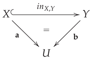
An object in a category is called initial if there exist for any object A in exactly one morphism from into A often denoted by and called initial morphism for A. The empty set ∅ is the initial object in while for any set A the corresponding initial morphism for A is simply the inclusion map .
A category is small if the collection , and thus also the collection , is a set. is the category of all small categories. and are not small! A category is locally small if is a set for all objects A and B in . and are locally small! is the category with all small categories and categories like and as objects.
For a category we denote by the underlying reflexive graph, i.e., in we simply forget that there is a composition operation in . Obviously, each functor comprises a corresponding reflexive graph homomorphism between the underlying reflexive graphs. Not every reflexive graph homomorphism establishes, however, also a functor because a reflexive graph homomorphism is not required to be compatible with composition.
We consider also reflexive graph homomorphisms from reflexive graphs H into the underlying reflexive graph of categories and denote them by (compare the concept of a model of a graph in a category in [9]). The traditional definition of natural transformations between functors can be reused to define natural transformations between those reflexive graph homomorphisms .
Natural Transformations:
If and are natural transformations, the vertical composition of and is denoted such that for each , .
Also, if , , are functors and is a natural transfomation, the horizontal compositions of with , and with are represented as and such that for each , , whereas .
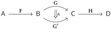
The traditional definition of natural transformations between functors can be reused to define natural transformations for all (!) reflexive graph homomorphisms between the underlying reflexive graphs of categories (compare [9]).
Institutions: The concept of Institution introduced by Goguen and Burstall [19] formally captures the notion of logical systems. A similar proposal of an abstract concept of a logic had been given already by Barwise [21]. The following definition can be found in [19,20]: An institution is given by a category of (abstract) signatures, a functor , a functor and a -indexed family of satisfaction relations such that for each morphism in , the Satisfaction Condition
holds for each (abstract) model and (abstract) sentence.
Name spaces: It is under-communicated that the definition of morphisms between concrete institutions often relies on the implicit assumption that the syntactic entities of both institutions are build upon the same stocks of symbol identifiers. We restrict ourselves to finitary syntactic entities. Therefore, we assume that all considered first-order institutions are build upon a certain choice of three enumerable and disjoint name spaces:
- A set of names for operation symbols.
- A set of names for predicate symbols.
- A set of names for variables which is equipped with a fixed total order.
We choose to be the totally ordered set .
In the general LoSiC-terminology, introduced in [1], all institutions share the same base category.
3. Basic Concepts and Constructions in First-Order Logic
Relying on hom-sets, instead of Cartesian products, we recast in this section the definitions of the basic syntactic and semantic concepts of unsorted first-order logic.
3.1. Signatures and Structures
In this paper about first-order logic we use the traditional term signature instead of the neologism footprint coined for the general setting in [1]. Since we will neither misuse constant symbols to encode variables nor to encode elements of carriers of first-order structures, we can restrict ourselves to finite signatures only.
To achieve category-independent definitions, we require in [1] that the arities of predicate and operation symbols are defined by means of "variable declarations". In LoSiC-terminology all share the same category of "variable declarations". For unsorted first-order logic we simply define to be the set of all finite subsets of (considered as a discrete subcategory of ). We will simply use the term set of variables, instead of "variable declaration", for those finite subsets .
Definition 1
(Signature). Asignature is given by
- a finite set of predicate (relation) symbols,
- a finite set of operation (function) symbols, and
- arity functions , , where is a singleton for all . We assume that and are disjoint for all (compare [22]).
We intend to be as precise as possible concerning notations. Therefore, we include in the paper many remarks devoted to bridge the notational gap between the category-independent notations in [1] and the traditional notations in first-order logic. We tried our best, but still the notations may become too heavy at some places and we apologize for this. Another essential part of the many remarks is devoted to explain the new or modified concepts and to discuss their relationships to traditional concepts.
Remark 1
(Representation and Syntactification of Sets of Variables). Any set X of variables inherits a total order from . This allows us to represent X as an n-tuple of variables with thecardinalityof X and denoting the i-th variable in the totally ordered set X for all .
In such a way, we also can syntactically encode the set X of variables by the string of symbols . We use the delimiter signs … to indicate that the expression between the delimiters is a string of symbols. So, the delimiter signs are not constituents of syntatctic entities and we may just drop them if convenient.
Example 1
(Signature). We define a signature to describe and reason about structures with an irreflexive order relation, constants zero and one as well as binary operations addition and multiplication as follows:
- with arity ; and
- with input arities , and output arities .
In unsorted first-order logic we traditionally assume that all structures do have a non-empty carrier set! This is a crucial prerequisite to achieve soundness of the traditional lazy approach to first-order deduction that avoids, as much as possible, to explicitly handle (sets of) variables! So, in LoSiC-terminology all institutions share the same category of potential carriers of structures. After we this is clarified, we are going to define the category of structures for a given signature .
Definition 2
(Structure). For a signature a-Structure is given by
- a set U, called thecarrierof ,
- a family ofpredicates, i.e., subsets ofvalid assignmentsfor the predicate symbol in , and
- a family ofoperations (functions) in .
Remark 2
(Notation of Structures). We draw attention to a notational subtlety: We denote a structure and its underlying carrier set with the same letter but in different fonts. For the Σ-structure we use the calligraphic font and for the carrier set we are using the normal font U. Note, that the superscripts for the predicates and operations are therefore also calligraphic!
Remark 3
(Hom-set vs. Cartesian Product). Attention! We don’t follow the traditionally way to use Cartesian products to define predicates and operations. We use hom-sets instead!
The category is small thus the hom-set is a set and can be treated, in a "self-referential way", as an object in ! Besides many other specialties of , we do have that (X,U) can be considered to "be the same" as the set of all maps from X to U, which is, in turn, anexponential objectin . The exponential object is, however, also a (categorical) product in . Especially, it is isomorphic to the Cartesian product with !
For nearly any other category the equivalence between the concepts hom-set, exponential object, and (categorical) product vanishes! It took us a while to realize the disappearance of this "self-evident equivalence" in other categories and to find out, that only the hom-set perspective allows us to generalize first-order logic to arbitrary categories in the way it is outlined in [1].
Remark 4
(Representation of Variable Assignments). We consider a set X of variables with . For a given set U, a map will be also called(variable) assignment of X in U.
There is a bijection between the set of all assignments of X in U and the Cartesian product . That is, anyassignment can equivalently be represented as an n-tuple with for all where the are defined as in Remark 1.
We utilize both notations and synonymously. Note, that in case of the empty set the only element in is represented by theempty tuple.
Due to the hom-set perspective the translation of variable assignments along homomorphisms can be expressed by simple composition thus the homomorphism conditions appear in an unconventional but quite adequate form.
Definition 3
(Homomorphism). A-homomorphism between two Σ-structures and is given by a map such that
- 1.
- implies for all and all assignments , i.e., the post-composition map , with for all , restricts to a map .
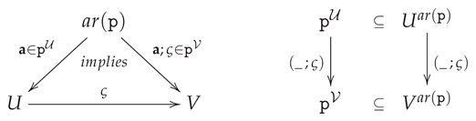
- 2.
- for all and all input assignments , i.e., .
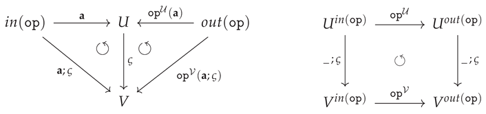
Remark 5
(Notation of homomorphisms). The convention to denote a Σ-structure and its carrier set by the same letter but in differents fonts, allows us to distinguish as well between different kinds of morphisms: When we write , we mean a map. When we write, however, , we mean a Σ-homomorphism. In such a way, the notation carries the implicit information/assumption that ς is not only a map but satisfies, in addition, the homomorphism conditions.
Example 2
(Structures and Homomorphisms). For the sample signature in Example 1 with , we consider three Σ-structures:
- 1.
-
with the set of all natural numbers as carrier.
- is the usual irreflexive order on : iff .
- is the natural number zero: for the only element . is the natural number one: .
- is addition of natural numbers, i.e., for all we do have . is multiplication of natural numbers: for all .
- 2.
-
with the set of all rational numbers as carrier.
- is the usual irreflexive order on : iff .
- is the rational number zero: for the only element . is the rational number one: .
- is addition of rational numbers, i.e., for all we do have . is multiplication of rational numbers: for all .
- 3.
-
with the power set as carrier.
- is the irreflexive inclusion order: iff .
- is the empty set: for the only element . is the set : .
- is union of sets, i.e., for all we do have . is intersection of sets: for all .
The inclusion map obviously defines a Σ-homomorphism , while the embedding map assigning to each natural number the singleton does not provide a Σ-homomorphism from to .
For any -structure the identity map obviously establishes a -homomorphism . Moreover, it can easily be shown that for any -homomorphisms , the composition of the underlying maps becomes also a -homomorphism . Identity and associativity law for composition are inherited from the category , thus we obtain the category of all -structures and all -homomorphisms denoted by .
3.2. Terms and First-Order Expressions: Syntax
We consider terms and first-order expressions as syntactic entities and define them as finite strings of symbols. To distinguish terms from meta-level expressions, such as , we will use angle bracket symbols , instead of parenthesis , to build terms. As discussed in Remark 1, we will use delimiter signs … to indicate that the expression between the delimiters is a string of symbols.
The following is a traditional inductive definition of terms similar to [5,6,7] and relies on the notational conventions in Remark 4:
Definition 4
(Terms: Syntax). The set of all-termsover a set X of variables is the smallest set of strings of symbols such that
- Variables:
- for all ;
- Constants:
- for all with ;
- Operations:
- for all with and all assignments in .
Note that the assignments , assigning to each element in X the string constituted exactly of this single symbol, define an injective map : .
Note further, that each operation symbol with is reborn as the -term with the as in Remark 4.
Examples of terms can be found in Example 3 (Expressions: Syntax).
Remark 6
(Terms: Inclusions). We do have whenever . For a set X of variables not every Σ-term in "syntactically contains" all the variables in X. The set of all variables in X, "syntactically appearing" in a Σ-term , is the smallest subset such that . Inductively, we can define as follows: , and .
Remark 7
(Syntactification of Substitutions). A variable assignment of the form will be also called a-substitution (declaration). Due to Remark 4, we can uniquely represent any Σ-substitution by an n-tuple of terms where .
What we implicitly did in Definition 4, is to introduce the correspondingsyntactic encoding of the substitution as a string of symbols.
For the injective map : we get with variables due to Remark 1. In case of the empty set the only element in is represented by theempty tuple thus we have .
We introduce first-order expressions as the basic syntactic entities in our formalization of the informal concept of an "open formula". As syntactic entities we define them as strings of symbols relying on the notational conventions in Remark 1 concerning the syntactic representation of finite sets of variables and in Remark 7 concerning the syntactic representation of substitution declarations.
Definition 5
(Expressions: Syntax). For a signature , we define inductively and in parallel a family of sets of(first-order) -expressions on X, in symbols, where X varies over all sets of variables, i.e., all elements in :
- 1.
-
Atomic expressions:
- (a)
- Equation: for any Σ-terms .
- (b)
- Relational Atom: for any and any .
- 2.
- Everything: for any set X of variables.
- 3.
- Void: for any set X of variables.
- 4.
- Conjunction: for any expressions and .
- 5.
- Disjunction: for any expressions and .
- 6.
- Implication: for any expressions and .
- 7.
- Negation: for any expression .
- 8.
- Quantification: and for any expression and any proper inclusion .
Remark 8
(Expressions: Indexed vs Fibred Syntax). We construct in Definition 5 a -indexed family of sets, i.e., a map . The elements of are expressions on X. Obviously, there are for any expression infinite many different sets X of variables such that ! The notation simply encodes the "meta-level statement" and serves, at the same time, as a notational means to describe the disjoint union of all the sets as the set .
So, the syntax of expressions is described in two equivalent versions - theindexed version and thefibred versiongiven by and the projection with for all . We will utilize both versions in parallel!
Remark 9
(Syntax of expressions). Every predicate symbol is reborn as the Σ-expression since with according to Remark 7.
There are three changes/corrections compared to the category-independent Definition 8 of expressions in [1] where quantification is defined by means of morphisms since morphisms are the only ingredients we do have available in arbitrary categories.
First, we do not use arbitrary maps between sets of variables but only proper inclusion maps in quantifications. Second, these inclusion maps are not considered to be morphisms in the category of "variable declarations" for the institutions of statements defined in Section 4.1. (This is a correction!) Third, we adapt the traditional notation for quantification, i.e., we represent the proper inclusion maps by the complements in . Be aware, that the sets X, are disjoint and that Y can be reconstructed as their union .
Remark 10
(Free and Bound Variables). Relying on Definition 4 and 5, we can inductively define for any expression the set of allfree variables"syntactically appearing" in and the set of allbound variablesin . The basic case "Atomic expressions" is given by Remark 6 for free variables and the fact that terms do not have bound variables. Induction passes trivially through the con nectives. The essential deduction step is "Quantification".
Attention, the definition of quantification in Definition 5 ignores the free variables in . So, it may happen that none of the variables in actually appears as a free variable in !
We witness here a kind of "methodological accident" in the sense that the instantiation of our category independent approach to quantification in [1] reinvents, in the special case of traditional first-order logic, a well-known principle.
Our approach, to explicitly declare first all the variables , which are available, before actually constructing expressions using only the variables in X, together with our requirement for quantification has a subtle but important consequence. If then all the free variables in are contained in X, i.e., , and none of the variables in X appears as a "bound variable" in , i.e., . Other variables than the ones in X can appear, however, multiple times as bound variables in but only in non-overlapping "sub-expressions". These restrictions correspond toBarendregt’s variable conventionfor the λ-calculus (see [18], p. 26):
- bound variables are distinct from free variables, i.e., , and
- all binders bind variables not already in scope, i.e., in case of quantification with and .
To say it the other way around: Any traditional "well-formed formula", in the sense of [4] for example, complying with Barendregt’s variable convention corresponds to an expression in the sense of Definition 5 since the convention ensures that we can unambiguously construct the proper inclusions we need to define the case Quantification in Definition 5 (see also Remark (9)).
Compliance with Barendregt’s variable convention ensures that we can characterize as the smallest set Z of variables such that .
Lemma 1
(Reducing Variable Declarations). For any set X of variables and any Σ- expression , i.e., , we also have , i.e., , for all sets Z of variables with .
Proof.
By induction on expressions according to Definition 5. For atomic expressions the claim is obvious since for any if , due to Remark 6. Induction passes trivially through the connectives.
In case of quantification with let Z be arbitrary with . Due to Definition 5 and the definition of free variables in (1), we get with and thus . By Induction Hypothesis, and thus due to Definition 5. □
Remark 11
(Everything and Void). We consider ⊤ and ⊥ not aslogical constantsbut asbuilt-in nullary predicate symbols, i.e., . Therefore, we are not using traditional constant symbols likeTorF, for example. Built-in, means, especially, that ⊤ and ⊥ do have a fixed semantics for any Σ-structure , namely and . Be aware, that the string in and encodes the initial morphism . Analogously, the equation symbol "=" represents a binary built-in predicate symbol with arity and a fixed semantics in any Σ-structure. Finally, built-in means that none of the symbols appears in any of the sets , or .
Remark 12
(Closed expressions: Syntax). Σ-expressions of the form will be calledclosed -expressions. They represent nullary derived predicates that can be either valid or not valid in a given Σ-structure (compare Remark 11 and Remark 16).
Example 3
(Expressions: Syntax). We discuss some Σ-expressions for our sample signature with , in Example 1.
The following closed Σ-expression, which we identify by the "auxiliary name" ,
claims that the order relation is strict monoton w.r.t. addition. We can also express De Morgan laws
Our main methodological point is, however, to consider expressions as syntactic representations ofderived predicates,enabling us to denote properties in an anonymous way (analogously to "anonymous functions" in functional programming).
We may, for example, define the property "even" by the following Σ-expression
,
which we consider as a derived predicate with arity and "auxiliary name" . We may be also interested to define the property "minimum"
and the property "local minimum"
.
Or, we want to have the concept "immediate successor" at hand
.
We may be even interested to talk about "prime numbers"
.
We may also introduce a tertiary predicate "sum" representing the graph of the addition operation
.
Remark 13
(Role of Auxiliary Names). The auxiliary names , , , , , , in Example 3 are not auxiliary predicate symbols! They are shorthands for Σ-expressions and live on the "meta-level". They are something likemacrosin assembly programming. The auxiliary names bring us closer to the praxis of "working mathematicians":
- We define new properties/concepts and give them a name to be able to formulate our statements in a more natural language style, like "the sum of two even numbers is also even" for example.
- To formally prove those statements, we have to unfold our definitions. In assembly programming they use the termmacro expansionfor this kind of unfolding.
- On the other hand, we need a mechanism to "fold" our proofs into those natural language like statements.
A first variant of such a "folding of proofs" is discussed in Section 8.2.
3.3. Terms and First-Order Expressions: Semantics
As mentioned in Section 1, the semantics of a -term in a given -structure should be a derived operation. To define those operations, we consider the evaluation of -terms in -structures: Let a -structure be given. Based on Definition 4 and employing the fixed semantics of all operation symbols in F, we can inductively extend any assignment of a set X of variables in the carrier U to a map such that

This allows us to define the semantics of a -term in a -structure as the map defined by for all . We call the derived operation in represented by t. Each variable represents a projection. We can go even further: Any -substitution defines a derived operation in (in the opposite direction!) with
Since is a singleton, the inclusion map represents a constant operation . Moreover, the canonical injective map : represents the identity map on :
Following a popular and convenient tradition in logic (see [3], p. 66) we define a satisfaction relation between assignments of a set X of variables in a -structure and -expressions on X. We say that " is a valid assignments for " or " is valid for ".
Given an inclusion , we say that an assignment is an extension of an assignment to Y if, and only if, .
Definition 6
(Satisfaction Relation: Assignments and Expressions). For a signature , we define inductively and in parallel for an arbitrary, but fixed, a Σ-structure asatisfaction relation between assignments of a set X of variables in and Σ-expressions on X. X varies over all sets of variables, i.e., all elements in .
- 1.
-
Atomic expressions:
- (a)
- Equation: iff for .
- (b)
- Relational Atom: iff for .
- 2.
- Everything: for all
- 3.
- Void: for none
- 4.
- Conjunction: iff and
- 5.
- Disjunction: iff or
- 6.
- Implication: iff implies
- 7.
- Negation: iff not
- 8.
-
Existential quantification: iff there exists an extension of to Y such thatUniversal quantification: iff for all extensionsof to Y we have
We follow the "methodological imperative" that every syntactic entity should have a semantics in any structure. The semantics of a set X of variables in a -structure is simply the set of all assignments of X in U.
We consider first-order -expressions as syntactic representations of derived predicates, i.e., the semantics of a -expression in should be a subset of . The satisfaction relation defined in Definition 6 can be equivalently represented by those subsets. For all sets X of variables, all -structures and all -expressions we set
We can, however, also define the hom-set predicates independent of Definition 6, in a more compact and structured way, relying on the partial orders , the respective Boolean algebras and the monotone shift, existential and universal operators introduced and elaborated in Appendix A.
Definition 7
(Expressions: Semantics). The semantics of Σ-expressions in an arbitrary, but fixed, Σ-structure is defined inductively:
- 1.
-
Atomic expressions:
- (a)
- Equation: for is nothing but the equalizer of the derived operations .
- (b)
- Relational Atom: for .
- 2.
- Everything:
- 3.
- Void:
- 4.
- Conjunction:
- 5.
- Disjunction:
- 6.
- Implication:
- 7.
- Negation:
- 8.
-
Existential quantification:Universal quantification: .
Remark 14
(Expressions: Indexed vs Fibred Semantics). In view of Remark 8, we construct in Definition 7 an -indexed family of "natural transformations". For each Σ-structure we define a -indexed family of maps which establishes a "natural transformation" between the map and the map assigning to each set X of variables the power set
An equivalent, more fibred view is that the assignments define for each Σ-structure a map from into with where is the projection from into . Keep in mind that all the hom-sets in a category are assumed to be disjoint!
Remark 15
(Expressions: Semantics). As mentioned in Remark 9, every predicate symbol is reborn as the Σ-expression with . Definition 6 or 7 and Equation (5) ensure that also their semantics coincides .
The universal quantification is trivially valid for if there is no extension of to Y at all, while the existential quantification is not valid, in this case.
Two expressions and aresemantical equivalent, in symbols, if, and only if, for all Σ-structures . Definition 7 ensures that we do have the usual semantic equivalences available. In particular, conjunction and disjunction are associative; thus we can drop, for convenience, the corresponding parenthesis.
Remark 16
(Closed expressions: Semantics). We consider a closed expression (see Remark 12). is a singleton with the initial morphism as the only element. In such a way, we have either , i.e., , or , i.e., .
Example 4
(Expressions: Semantics). For the sample signature in Example 1 with , we consider the three Σ-structures , and in Example 2 and the derived predicates in Example 3.
For the closed Σ-expression we do have , and , i.e., addition is strict monoton in and but not in .
Conversly, we have for that , and , i.e., addition distributes over multiplication only in .
For we do have , and , . So in and all elements are "even".
For and we do have , and .
For we do have , and .
Moreover, we have , and .
4. First-Order Logics of Statements in Context
We are not addressing signature morphisms in this paper thus we do not recapitulate the corresponding parts from [17]. To make the paper sufficiently self-contained and accessible, we adapt and revise, however, in this section those parts from Section 5 and 6 in [17] to the case of traditional unsorted first-order logic which are relevant for the analysis of deduction calculi. Compared to [1,17], we elaborate, moreover, in addition and in more detail the hom-set predicate perspective on definitions, constructions and results, as we already started it with Definition 6 versus Definition 7 (see Appendix A).
4.1. Institutions of Statements
In this subsection we construct for each signature an institution of statements . Compared to the general case in [1], we consider only the variant with the full spectrum of first-order expressions and with the whole category of -structures as semantics . Therefore, we only need a simplified version of the construction of institution of statements as visualized in Figure 1.
Contexts are the (abstract) signatures in an institutions of statements. In the case of unsorted first-order logic all share the same base category and the same category of contexts which simply are the category of sets: . As common category of variable declarations we choose the set of all finite subsets of (considered as a discrete subcategory of ).
The soundness of deduction calculi for traditional unsorted first-order logic relies on the assumption that all -structure do have a non-empty carrier. Therefore, all institutions share the same category of potential carriers of structures.
Note, that the proper inclusions reflect the intended role of contexts to establish a bridge between syntax and semantics.
Remark 17
(Contexts in the Wild). Contexts are meant to establish a bridge between meta-level syntax (signatures, constant symbols, variables, terms, expressions) and semantics (structures and their carriers). In addition, we want to offer a home for those entities, being around in logic, which neither properly belong to meta-level syntax nor to semantics.
Demonstrating the bridge feature, we will utilize in the Section 7 and Section 8 sets of variables in the role of contexts. On the other hand, sets of (names for) elements in carriers can also take the role of contexts as outlined in the discussion ofelementary diagramsin Section 5.1.
Other examples of contexts, we do have in mind, are sets G ofgeneratorsin Group Theory, sets O ofliteralsin PROLOG, sets ofindividual names (nominals, objects)in Description Logic [13], sets ofHenkin constantsand so on. Contexts can also accommodateSkolem constants.
4.1.1. Institutions of Statements: Sentence and Model Functor
Statements in context are the (abstract) sentences in an institutions of statements.
Definition 8
(Statement). A-statement in a context is given by a set X of variables, a Σ-expression and abinding map. is calledatomicif is an atomic expression, i.e., an Equation or a Relational Atom.
By , we denote the set of all Σ-statements in K and by the obvious projection map. is the set of all Σ-statements in K for an arbitrary, but fixed, set X of variables.
Remark 18
(General statements and closed formulas). For any closed Σ-expression (see Remarks 12 and 16) there is a unique initial morphism ; thus, we have for any context K and all Σ-expressions . We call ageneral statement in K.
From all the general statements sharing the same closed expression , only the general statement in the empty context ∅ is the proper formal counterpart of traditionalclosed formulasin institutions of statements!
Example 5
(Context and Statement). For the sample signature Σ in Example 1, we define the contexts and . We can consider the elements in G as "number literals" in the sense of PROLOG or simply as elements of the carrier of the Σ-structure .
We adapt the encoding of assignments from Remark 4 and use for Σ-statements the shorthand notation . Instead of expressions , we will also use auxiliary names for expressions, as introduced in Example 3. If is a “reborn predicate symbol” (see Remark 9), we may use the traditional notation instead of .
and are Σ-statements in K with relational atoms. Σ-statements in K with equations are , , , and Σ-statements in K with auxiliary names are, for example, , , , .
Attention!We are not substituting variables by elements of contexts! Therefore, we can not write, for example, instead of .
Remark 19
(Statements in the Wild). We continue Remark 17. In Group Theory a statement in context G is called adefining relationbetween the generators in G and is, in fact, an equation bound to G. In Logic Programming a statement in context O is an atomic relational statement and usually called afactabout the atoms in O. In Description Logics they use the termrole assertionfor statements in context.
The "binding trick" starts to pay off. It allows us to encapsulate the relatively intricate construction of first-order expressions in the sense that we don’t need "substitutions" to define the translation of statements.
Any morphism in induces a map defined by simple post-composition for all statements in K:
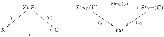
We do have and thus, equivalently said, that restricts to a map for every set X of variables.
Associativity of composition in ensures that the assignments and define a functor . This is the sentence functor of the institution .
Example 6
(Translation of Statements). For the contexts and from Example 5, we consider the map given by the assignments .
The statements in K from Example 5 are simply translated by means of the map to the following statements in context G. translates to and to .
translates to , to and to .
Finally, the Σ-statements in context K, , and with auxiliary names, are translated to , , and , respectively.
Interpretations of contexts are the (abstract) models in an institution of statements.
Definition 9
(Context interpretations). A-interpretation of a context is given by a Σ-structure in and a map .
A morphism between Σ-interpretations of K is given by a Σ-homomorphism such that for the underlying map .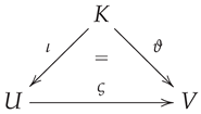
For any context K in , we denote by the category of all Σ-interpretations of K and all morphisms between them and by the obvious projection functor.
Note, that is an isomorphism and compare the later Remark 20. Any morphism in induces a functor defined by simple pre-composition for all -interpretations of G:

For any morphism between two -interpretations of G the same underlying map establishes a morphism between the corresponding two -interpretations of K, thus we have
Equivalently said, the functor restricts to a functor with the pre-composition map as the underlying map on objects.
Associativity of composition in ensures that the assignments and define a functor . This is the model functor of the institution .
4.1.2. Institutions of Statements: Satisfaction Relation and Satisfaction Condition
The last two steps, in establishing an institution, are the definition of a satisfaction relation for interpretations and statements and the proof of the so-called satisfaction condition. The satisfaction relation is simply provided by the satisfaction relation for assignments and expressions, as defined in Definition 6.
Definition 10
(Satisfaction Relation: Interpretations and Statements). For any context K, any Σ-statement in K and any Σ-interpretation of context K we define:
If , we say that ι is avalid interpretationfor in or that is valid for the interpretation ι in .
Analogously to (6), the satisfaction relation in Definition 10 allows us to define the semantics of statements in -structures. For all sets X of variables, all -structures and all -statements in a context K we set
Definition 10 implicitly relies on pre-composition maps thus we can define for all -structures the semantics of -statements in a context K independent of Definition 10 by
utilizing the shift operator according to Appendix A.2.
Remark 20
(Validity of General Statements). If , we do have for any Σ-structure exactly one interpretation thus for any "closed formula" (see Remark 18) means nothing but that the closed formula isvalid in in the traditional sense.
Moreover, the validity of general statements issemantically context independentin the following sense: For any context K, any Σ-structure , any Σ-interpretation of K in and any closed expressions , we have due to the uniqueness if intitial morphisms:
Example 7
(Interpretation and Satisfaction). The reader may check with help of Example 4, that the map in Example 6 is defined in such away that all the Σ-statements in context from Example 6 are valid for the interpretation of the context K in the Σ-structure from Example 2!
In contrast, only the Σ-statements , and in K are valid for the interpretation in where assigns to each natural number the singleton . Note, that the Satisfaction Condition in Corollary 1 allows us to show this claim by checking that the translated statements , , in context G are valid for the interpretation of G in .
After we developed everything in a systematic modular way, we obtain the satisfaction condition "for free", namely by associativity of composition in .
Corollary 1
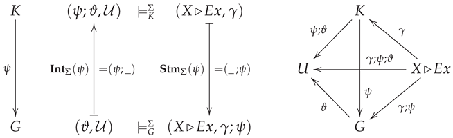
(Satisfaction Condition). For any morphism in , any Σ-statement in context K and any interpretation of context G in a Σ-structure , we have:
Proof.
Due to the definition of the functors and , we obtain the commutative diagram, above on the right, thus the satisfaction condition follows immediately from Definition 10 (Satisfaction Relation: Interpretations and Statements) and associativity of composition. in □
We can also independently prove the satisfaction condition on the level of hom-sets. Exemplifying a general result about an equivalent characterizations of the satisfaction condition for institutions (see the concept institution frame in [23,24]) and due to the properties of the maps and concerning restrictions (see (7)), the satisfaction condition in (13) is equivalent to the requirement that for any context morphism , any -structure and any set X of variables the diagram below on the right commutes.

For any -statement we get indeed
Summarizing all definitions and results, we obtain for each signature the Institution of -Statements in Context not only comprising "closed formulas", as it is traditionally the case [19,20], but also "open formulas"!
Since we only consider, in the remaining part of the paper, one single arbitrary but fixed signature we may drop the superscript in whenever it is convenient.
4.2. Substitutions
Substitutions are not relevant for utilizing a logic as a specification formalism. As also mentioned in [20], substitutions are, however, an important logical device for deduction. In this section we investigate substitutions and develop corresponding extensions of constructions and results necessary and sufficient for deduction.
4.2.1. Categories of Substitutions
The simple natural idea is to extend the family of sets of variables by substitutions. For any signature the small category is defined as follows:
- Objects:
- are all sets X of variables, i.e., ;
- Morphisms:
- in are given by -substitutions ;
- Identities:
- on sets X are given by the canonical maps : ; and the
- Composition:
- of two morphisms , in is given by the -substitution where is the inductive extension of such that
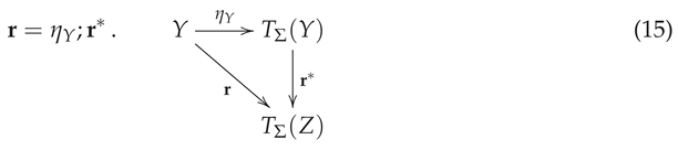
Note, that describes nothing but the application of the -substitution to all -terms over Y! We can inductively prove that
thus the composition of substitutions is associative, and we get indeed a category.
Remark 21
(Lawvere Theories). The tentative reader may have realized that the categories are nothing but so-calledsyntactic Lawvere theories[25,26,27]. We will, however, not walk further into the realm of "Categorical Algebra" and "Functorial Semantics". We will neither utilize the fact that the categories are finite product categories nor reconstruct (Σ) as a subcategory of the functor category in case of signatures Σ without predicate symbols!
Remark 22
(Kleisli Morphisms). It is a common practice to describe substitutions as morphisms of the Kleisli category of a "term algebra adjunction". In such a way, we would get the extension of assignments in (3) and the application of substitutions in (15) as well as their compatibility "for free". See the discussion of "internalization of terms" and of substitution calculi in [22].
To stay closer to traditional presentations of logics, we rely instead in this paper on explicit inductive definitions (located on the meta-level). Another reason is, that in the many-sorted case some of the necessary constructions and results, as the translation of terms along signature morphisms and the composition of term translations for example, can anyway not be obtained by means of term algebra adjunctions (see [17])!
4.2.2. Substitution Application for Expressions
Analogously to terms, we would also like to extend the map , constructed in Definition 5, to a functor . We can indeed define for all -substitutions a map describing the application of the substitution to -expressions on X. Due to the presence of quantification, the assignments will be, however, not functorial on the nose as we will discuss below.
There seems to be no way out! As long as we do not utilize something like de Bruijn indices [28] to avoid named bound variables, we have to deal, in one or another way, with the problem that substitution application may cause an unintended interaction between free and bound variables. One approach to avoid such an unintended interaction is to inductively define a binary meta-level predicate stating when a substitution is legal for a certain expression as it is done, for example, in [4]. We will, however, not adapt this approach, since we would end up with partial substitution maps .
Another approach is to use α-conversion, i.e., renaming of bound variables, in such a way, that we obtain total substitution maps. We will define the application of a substitution to expressions, according to the inductive definition of expressions in Definition 5, thereby establishing a stepwise inductive variant of an implicit -conversion.
To meet the proper inclusion condition for Quantification in Definition 5, we must use non-symmetric sums when defining substitution application in case of Quantification. That is, for any two sets of variables we must choose a set which is a sum in such that the left injection is an inclusion .
General Assumption: If and are disjoint, we simply choose .
Definition 11
(Substitution Application for Expressions). For any signature Σ the family of maps with a Σ-substitution is defined inductively and in parallel by the following assignments:
- 1.
-
Atomic expressions:
- (a)
- Equation: for any with given by (15).
- (b)
- Relational Atom: for any and any substitution with given by (15).
- 2.
- Everything:
- 3.
- Void:
- 4.
- Conjunction:
- 5.
- Disjunction:
- 6.
- Implication:
- 7.
- Negation:
- 8.
- Quantification: and for any expression and any proper inclusion where and thus . The extended substitution is constructed as a cotuple (by case distinction). Remind Remark 6 and that Y is the sum of X and in since .
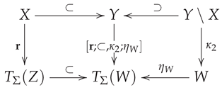
There seems to be no choice of non-symmetric sums in such that the assignments and define a functor from into since for any -substitutions , the maps and coincide, in general, only for -expressions without quantifications. For a -expression on containing quantifications, the two -expressions and may be syntactically different. They are, however, "the same up to -conversion". Especially, it can be shown that they are semantically equivalent.
Lemma 2
(Semantic Equivalence). For Σ-substitutions , the maps and are semantically equivalent in the sense that
We will define and investigate -conversion in Section 6.3. To describe deduction in first-order logic we will need -conversion anyway, independent of the fact if the assignments and define a functor from into or not. So, let us formally grasp what we have at hand besides Lemma 2.
4.2.3. Substitution Application vs Derived Operations
According to (3) and (4), any -substitution represents for any -structure a derived operation in the opposite direction with for all assignments . For any -substitution and any assignment it can also inductively shown that

This entails
That is, composition in syntactically represents the composition of derived operations! The equations (18) and (5) ensure that for any -structure the assignments and define a contra-variant functor as the semantic counterpart of the reflexive graph homomorphisms .
and are not fully matching the "original institution pattern". Nevertheless, we do have a corresponding satisfaction condition: For any -substitution , any -expression , any -structure and any assignment it holds that
This is our reconstruction of the statement in Proposition 5.8 in [20].
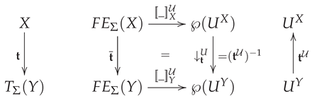
Once more, we can independently describe the traditional satisfaction condition in (19) by means of hom-sets. We extended the map in Remark 8 to a reflexive graph homomorphism . Correspondingly, we can extend for each -structure the map in Remark 14 to a functor obtained by composing the contravariant functor with the contravariant powerset functor that relies on the formation of pre-images.
The satisfaction condition in (19) is then equivalent to the requirement that for any -structure the -indexed family of maps establishes a natural transformation : For any -substitution and , any -expression and any -structure it holds that
5. Sketches and Arrows between Sketches
Any institution gives us a corresponding category of presentations and an extension of the model functor of the institution to the category of presentations at hand [19,20]. We outline, adapt and extend this construction for Institutions of Statements.
5.1. Sketches and Diagrams
In the area of Algebraic Specifications those presentations are, for example, pairs of an algebraic signature and a set of (conditional) equations and are called specifications. [6,7,8]. In the different institutions of algebraic specifications and in the traditional institution of first-order logic [19,20] the "models" are whole structures.
In contrast, LoSiCs shift the perspective from whole structures to single interpretations of contexts in structures. Note, however, that this is not only a shift but also an enhancement of perspective since the "whole structure perspective" can be reconstructed by the restriction to empty contexts only (see Remark 20). Incarnations of this enhanced perspective are, for example, Ehresmann Sketches [9] and Generalized Sketches in the sense of Makkai [10] or in the sense of Diskin [11,12]. Generalized Sketches in the sense of Diskin have been shown to be an appropriate conceptual tool to formalize software models and to pave a way for a theoretical foundation of Model Driven Software Engineering [15,16]. To underline this enhanced perspective and the "historical roots" of LoSiCs, we use the term sketch, instead of presentation or specification.
Definition 12
(Sketch). For any signature a- sketch is given by a context and a set of Σ-statements in context K. is calledatomicif all the Σ-statements in are atomic meaning that is an atomic expression, i.e., an equation or a relational atom according to Definition 5.
Remark 23
(Sketches in the Wild). We continue Remark 19. In Group Theory we meet sketches as pairs of a set G of generators and a set R of defining relations between the generators in G. A sketch in Logic Programming is given by a set O of atoms and a set F of facts about the atoms in O. Sometimes one may also meet the termlogical database.
Finally, we find sketches in Description Logics as pairs with a set of individual names (nominals, objects) and a so-calledABoxof assertional axioms.
Definition 13
(Interpretations of Sketches). An interpretation of context K in a Σ-structure isa valid interpretationof the sketch in , in symbols, if, and only if, , due to (10), for all Σ-statements in . Be aware that the Σ-statements in may have different sets X of variables!
Analogously to the semantics of statements in (11), we can define the semantics of a -sketch in a -structure as the set of all valid interpretations of in :
For later references it is convenient to lift up the characterization of the satisfaction condition in (14) to arbitrary subsets of statements and, thus, to fully exemplify the concept of institution frame in [23,24]. For any context morphism and any -structure the diagram below commutes.
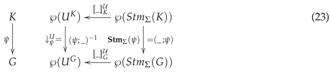
For any set of -statements in context K we get indeed
(Elementary) diagrams play an essential role in completeness proofs. We will not address completeness proofs in this paper. We want, however, shortly outline and discuss this additional motivation for introducing contexts.
We became familiar with diagrams not via Model Theory [2,3,20] but as a technique used in the construction of free algebras [6,7,29]. From this perspective diagrams arise as syntactic representations of structures. To obtain such a representation, we need, first, a mechanism to syntactically represent the elements of a given structure.
A widely used mechanism is to add for a given -structure "copies" of all the elements in the carrier U of as new auxiliary constant symbols to the signature (thus blowing up to an infinite entity in most cases) [2,6,20]. In contrast, Logics of Statements in Context generalize the approach in [7,29] which adapts the idea of generators and defining relations from Group Theory.
The elements of contexts are for us, in principal, neither constant symbols nor variables nor elements of carrier sets. Or, to put it the other way around: Of course we can use one and the same entity in different roles, but we should always be aware of the different roles and changes of roles! Contexts establish a bridge between syntax (constant symbols, variables) and semantics (elements of carrier sets), and we use them to define diagrams.
The first step in transforming a -structure into a -sketch is to transform the carrier U of into a context by introducing a syntactic duplicate for each element in U or by simply declaring that "we consider U in the role of a context".
In the literature we essentially find two variants of diagrams - an atomic variant [3,20] and a full variant [2]. Obviously, we can define two corresponding variants of sketch encodings of a -structure . The atomic variant is given by the -sketch
for the canonical interpretation of context the U in the -structure .
The full variant of the -sketch encoding of is obtained by droping the restriction "atomic". The interest reader may have a look at [1] for more concepts and results around sketch encodings. Especially, we discuss there a universal property of the canonical interpretation which is strongly related to Proposition 4.10 in [20].
5.2. Arrows between Sketches
In this subsection we revisit, revise, adapt and extend the discussions, definitions and results of the Subsections 5.2.3, 5.2.4 and 5.2.5 in [1]. Each -sketch has his own local context declaration thus arrows between sketches are established by context morphisms.
Definition 14
(Sketch Arrow). A-sketch arrowbetween two Σ-sketches and is given by a context morphism and denoted by . isatomicif all the Σ-statements in and are atomic. The category of all Σ-sketches and all Σ-sketch arrows is denoted by .
A Σ-sketch arrow is calledstrict, in symbols, if, and only if, with the statement translation defined in (7). is a functor thus the strict Σ-sketch arrows constitute a subcategory of .
In case and , we simply write and , respectively.
5.2.1. Sketch Morphisms
Sketch arrows are subject of two different, but dual, semantical conditions. First, any institution gives us a corresponding concept of presentation morphism at hand [19,20]. We discuss the corresponding morphism condition and, as a terminological sleight of hand, we will use the term sketch morphism and the notation to indicate that a sketch arrow is subject of the morphism condition.
Definition 15
(Satisfaction of Morphism Condition). A Σ-sketch arrow satisfies themorphism conditionfor a Σ-structure , in symbols, if the "forgetful map" in (14) restricts to a map , i.e., if or, equivalently due to Corollary A4, if .
Identity -sketch arrows trivially satisfy the morphism condition and satisfaction of the morphism condition for a -structure is, due to (A23) and the monotonicity of the operators , closed under composition in thus all -sketch arrows satisfying the morphism condition for a -structure constitute a subcategory of .
The syntactic strictness condition ensures the satisfaction of the morphism condition.
Corollary 2
(Morphism Condition by Strictness). We have for any Σ-structure , i.e., for any strict Σ-sketch arrow it holds that .
Proof.
For any strict -sketch arrow and any -structure we get indeed
□
5.2.2. Sketch Implications
The implication condition is the second semantical condition for sketch arrows. To motivate and elucidate this second condition we informally discuss the paradigmatic specification framework of conditional equations. An analogous discussion applies to the specification framework of Horn clauses (PROLOG).
The first crucial methodological observation is that conditional equations are not, and never have been, a lazy notation for closed formulas ! Conditional equations have been introduced and utilized as a conceptual tool of its own independent of first-order logic! One of the many motivations to coin the concept of LoSiCs was to develop a conceptual framework enabling us to precisely grasp the particular nature of conditional equations. In LoSiC-terminology conditional equations are a special kind of atomic sketch arrows
A conditional equation is satisfied in a -structure if, and only if, each solution of the premise in also is a solution of the conclusion .
The second observation is that we do have, at least, three well distinguished (!) syntactic entities that one could call "equation".
- Expression:
- First, we do have atomic expressions with their individual semantics in any -structure . This semantics is the set of all variable assignments solving the equation .
- Statements in Context:
- Second, there are for each atomic expression infinite many single statements in contexts where the semantics of in a -structure is the set of all interpretations such that solves the equation .
- Unconditional Assertion:
- Third, we do have for each atomic expression a sketch arrow which is valid in a -structure if, and only if, each solution of the "empty premise" , i.e., all variable assignments , solve the equation or, in other words, if t and r represent the same derived opperation in .
This conceptional triad "expression - statements in context - unconditional assertion" we do have in LoSiCs for any expression at hand!
Analogous to the morphism condition, we will use the term sketch implication and the notation to indicate that a sketch arrow is subject of the implication condition.
Definition 16
(Satisfaction of Implication Condition). A Σ-sketch arrow satisfies theimplication conditionfor a Σ-structure , in symbols, if, and only if, for all interpretations of P in it holds that implies the existence of an interpretation of context C in with such that .
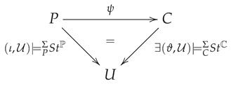
Obviously, we trivially have if there is no interpretation of context P in -structure at all. As discussed before, this may be the case in many-sorted logics due to the potential presence of empty sorts. In case and , we have if, and only if, each valid interpretation of the premise is also a valid interpretation of the conclusion .
By means of the existential operators from Appendix A.2, we can equivalently define the satisfaction of the implication condition as follows:
So, the morphism condition in Definition 15 and the implication condition are indeed dual semantical conditions! Analogously to the morphism condition, the characterization (25) ensures that all the -sketch arrows satisfying the implication condition for a -structure constitute a subcategory of .
We use the notation if both conditions are satisfied.
Due to Corollary 2, the equality in (26) especially holds for all strict -sketch implication!
Sketch implications enable us to specify and/or describe properties of -structures. The implication condition is the essential specification tool in specification frameworks of conditional equations [7,29], in specification frameworks of Horn clauses as well as in Makkai’s General Sketch framework [10]. In case of first-order logic, however, sketch implications do not add any "specification power" since the satisfaction of a -sketch implication in -structures can obviously be simulated by the satisfaction of a corresponding closed formula as long as and are finite (compare Section 5.2.4 in [1]).
5.2.3. Sketch Arrows and Injectivity
Besides specifying and/or describing properties of -structures, sketch arrows can be also utilized to specify and/or describe the structure of -sketches.
Definition 17
(Injectivity). A Σ-sketch isstrictly injective w.r.t. a -sketch arrow if, and only if, there exists for each strict Σ-sketch arrow a strict Σ-sketch arrow such that .
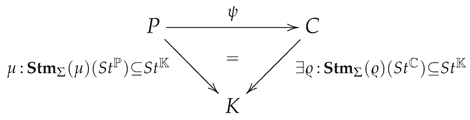
In Definition 23 in [1] we used, instead of "strictly injective", the attribute "closed" based on the intuition that is closed w.r.t. the application of as a deduction rule (compare the next subsection and [29]). Afterwards, we became more acquainted with the abstract concept of injectivity [30,31] and adapted therefore Diaconescu’s idea to indicate the restriction of the all-quantification in the definition of injectivity to a certain class of arrows by adding an adverb - "simply" on page 17 in [20] for the restriction to monic arrows. Since we only consider one type of injectivity in this paper, we simply drop the adverb "strictly" in most cases.
The satisfaction condition in ensures that the satisfaction of the implication condition in structures can equivalently be expressed by the strictly injectivity of sketch encodings of structures (24).
Proposition 1
(Implication Condition ≅ Injectivity). For any Σ-sketch arrow and any Σ-structure the following two statements are equivalent:
- 1.
- , i.e., satisfies the implication condition for .
- 2.
- The Σ-sketch encoding of is strictly injective w.r.t. .
Results, analogously to Proposition 1, are the corner stone for completeness proofs in specification frameworks of conditional equations [7,29]. In Makkai’s Generalized Sketch framework [10] there is no distinction between structures and sketch encodings and injectivity w.r.t. sketch arrows is the only conceptual tool for specification and/or description. Moreover, sketch arrows are the only tool for deduction thus results, analogously to Proposition 1, also are the corner stone for completeness results in [10]. Probably, related results also play a crucial role in completeness proofs in traditional first-order logic!?
5.3. Deducing Sketch Implications
There are, at least, three semantically sound mechanisms to deduce sketch implications from given sketch implications. First, we can simply obtain new (strict) sketch implications from given (strict) sketch implications by means of composition in . This procedure is sound since we have and thus also .
Second, we can apply a given sketch implication as a rule via sketch morphisms to deduce sketch implications. We discuss and validate this mechanism in this subsection. Third, we can apply a given sketch implication as a rule via substitutions to deduce sketchs implication. Rule application via substitutions is, however, only feasible for sketches where all bindings are identities. We postpone the discussion of this mechanism to Section 6.4.
We consider an arbitrary, but fixed, -sketch arrow . For any given -sketch and any -sketch arrow , called a match, we can construct a pushout of the underlying context morphisms , in .

As usual, the interpretation of a "syntactic pushout" in a chosen "universe" provides a "semantic pullback". In our case, we get for any carrier set U a pullback of hom-sets and pre-composition maps, as visualized in the middle square above, since for any interpretations , with there exist a unique interpretation such that and due to the "syntactic pushout" in the left hand square above. Note, that this is nothing but model amalgamation in the sense of the theory of institutions [20]. Compare also the amalgamation of algebras in [6].
We extend, in a minimal way, the pushout of context morphisms to a commutative square of -sketch arrows by defining with .
By definition, we obtain a strict -sketch arrow which always satisfies, according to Corollary 2, the morphism condition.
Corollary 3
(Morphism Condition for Instances 1). For any Σ-structure it holds that , i.e., we have .
In light of sketch implications, we construct for a given sketch implication and any sketch morphism a corresponding sketch implication which we may call the result of applying the rule ψ to via the match μ. We show the soundness of this procedure.
Proposition 2
(Rule via Sketch Morphism). For any Σ-structure with , i.e., , and , i.e., , it holds that , i.e., .
Proof.
If , the inclusion trivially holds. If , we consider an arbitrary . By assumption , we get thus there exists a with due to assumption . For the unique with and the fact and the satisfaction condition (23) for ensure with and thus , as required. □
It is maybe worth to mention, that Proposition 2 is related, in a certain sense, to the so-called "Extension Lemma" on page 223 in [6].
The semantic condition is not really feasible. However, Corollary 2 allows us to work, instead, with the stronger but pure syntactic condition "strict".
Corollary 4
(Rule via Sketch Morphism). For any Σ-structure with , i.e., , and any strict Σ-sketch arrow , i.e., , it holds that , i.e., .
In case , we may call the instance of with respect to the context morphism (!) .
In practice, we may be interested to also deduce strict sketch implications. For the strict variant with of the resulting -sketch, we also get for any -structure . To prove this, we need only to extend the last sentence in the proof of Proposition 2 as follows: For the unique with and the satisfaction condition (23) for ensures while the satisfaction condition for ensures . In such a way, we have with and thus , as required. By Corollary 2 we get, in such a way, a variant of Corollary 4 for the strict case.
Corollary 5
(Rule via Sketch Morphism - Strict). For any Σ-structure with , i.e., , and any strict Σ-sketch arrow , i.e., , it holds that , i.e., .
6. Licensing Laziness
In view of LoSiCs, notations in traditional first-order logic are "lazy" in the sense that there are neither explicit variable declarations nor are contexts explicitly considered. In this subsection we discuss how and under what conditions the traditional lazy notations can be recasted in a LoSiC-compatible way. In first-order deduction calculi we only deal with finite sets of finite formulas thus we will only need finite sets of variables in as variable declarations and as contexts for our analysis.
Let be a finite set of "well-formed formulas" in the traditional sense, as in [4] for example. The expressions in LoSiCs are well-formed formulas satisfying some syntactic restrictions. First, LoSiCs require that each well-formed formula has its own local declaration of free variables establishing its "interface" with the outside world. We could say that the traditional approach implicitly provides this "interface" in form of the set of all free variables syntactically appearing in B. Due to the "methodological accident", discussed in Remark 10, expressions in LoSiCs must comply with Barendregt’s variable convention thus we will, in general, not have , i.e., , in the sense of Definition 5. By a renaming of bound variables we can, however, transform any well-formed formula B into an equivalent expression with and .
In logic textbooks, as in [4] for example, they say that deduction calculi for first-order logic can inherit axiom schemata and rules from deduction calculi for Propositional Logic. There is, however, no formal explanation in what sense an open formula represents a proposition. In LoSiCs we try to repair this flaw by introducing statements in context which are statements about single (!) interpretations of contexts in a given structure and, thus, propositions in the sense of Propositional Logic.
Due to the lack of explicit variable declarations and explicit declarations of contexts, there also are no explicit bindings and context morphisms in traditional first-order logic. The only implicitly present morphisms are inclusion maps. We may consider as the implicit context of thus we could transform into a sketch with context X and the set of statements in context X. In alignment with traditional first-order logic, we can, however, in LoSiCs only combine expressions by Boolean operators but not statements in context! That is, we cannot represent an implication, like "" in traditional notation with , by a phrase like "" but only by a statement in context like with . Due to Barendregt’s variable convention this statement is only syntactically correct if the sets Y and are disjoint!
To be able to mimic the traditional free Boolean combination of well-formed formulas, we decide, therefore, to utilize a specific class of -sketches in our analysis of traditional first-order deduction calculi. We use only sets X of variables as contexts. We only consider finite -sketches with simple statements, i.e., statements of the form . In such a way, we adapt a strict separation of free and bound variables in the sense that we require . So, compared to the traditional approach, which simply works with arbitrary finite sets of arbitrary well-formed formulas, we propose three changes:
- 1.
- We declare an explicit context X with .
- 2.
- We require and adapt, in such a way, Barendregt’s variable convention.
- 3.
- We require, moreover, , i.e., a strict separation of free and bound variables.
We call a pair of a set X of variables and a finite set of well-formed formulas LoSiC-compatible or, synonymously, a -specification if it satisfies the conditions above, i.e., if can be seen as a representation of the simple -sketch with statements . The semantics of a -specification is defined by
for any -structure . The syntactic requirements 2. and 3. above are only of technical nature and cause no loss of generality! We have to ensure, however, that all constructions, relevant for deduction, preserve LoSiC-compatibility!
6.1. Reduction of Contexts
A first simple construction is the reduction of contexts. Given a -specification and a set Z of variables with , the pair is expected to also be a -specification and both pairs should represent the same semantic information.
Lemma 1 ensures that is a -specification too. That both -specifications and represent the same semantic information is ensured by Lemmma 3 below formally grasping the observation that the semantics of an open formula only depends on the free variables (compare Lemma 9.7 in [4] for example).
To prepare the proof of Lemma 3, we fix a crucial observation (that, unfortunately, vanishes in the many-sorted case). According to (A25), we do have for any carrier U that the projection map for any inclusion map between contexts is surjective thus we also have by (A24)
for the operators , and defined and elaborated in Appendix A.2.
Lemma 3
(Inclusion of Contexts). For any Σ-expression B and any sets Z, X of variables with and , the following two equivalent conditions for the inclusion map hold for all Σ-structures
Proof.
According to Corollary A3, the right condition always implies the left condition while the implication in the other direction is ensured by (29).
We prove the claim by induction on expressions according to the inductive definition of syntax of expressions in Definition 5 and of semantics of expressions in Definition 7.
For the case Relational Atom, we consider the substitution . The map , due to (15), is nothing but the inclusion claimed in Remark 6. The definition of derived operations by (3) and (4) entails for all and thus .
for means that there is a unique with and thus . Due to (17) and (18), this ensures that . In such a way, we get by Definition 7 and (A36). and, therefore, as required .
The case Equation can be shown in the same way since the equation symbol "=" can be seen to represent a built-in predicate with arity , as discussed in Remark 11, and a fixed semantics in any -structure .
Case Void is trivial since the preimage of the empty set is always the empty set and case Everything simply reflects that is a total (!) map.
The cases Conjunction, Disjunction, Implication and Negation are ensured since shift operators distribute over intersections as well as over unions and since they also are compatible with complements (see Appendix A.1 and (A13)).
We show case Quantification by means of the right condition in the lemma. For with let Z be arbitrary with . In such a way, we do have two chains of inclusions and with and thus due to (A23).
By Induction Hypothesis, , thus we get, due to Definition 7, for the inclusion chains and and therefore as required. □
We can straightforwardly generalize Lemma 3 to arbitrary -specifications.
Corollary 6
(Inclusion of Contexts). For any set Γ of Σ-expressions and any sets Z, X of variables with such that and are Σ-specifications the following two equivalent conditions for the inclusion map hold for all Σ-structures
6.2. Extension of Contexts
A second simple construction are context extensions. Let be a -specification and be the corresponding simple -sketch with . We consider a set Y of variables with .
The simplest idea is, obviously, to consider as the results of transforming along the inclusion map . However, to make this idea work we must, at least, require that is LoSiC-compatible. By assumption, we have thus the first condition of LoSiC-compatibility is trivially satisfied.
trivially implies . By assumption we also do have , thus the third condition of LoSiC-compatibility will be satisfied if, and only if, in addition to also holds. To say it with other words: Each variable in is required to be a notorious fresh variable in the traditional sense! That the "strong fresh variable condition" even entails the crucial LoSiC-compatibility condition , is ensured by the next lemma that is a complement to Lemma 1.
Lemma 4
(Extending Variable Declarations). For any set X of variables and any Σ- expression , i.e., , we also have , i.e., , for all sets V of variables with and .
Proof.
By induction on expressions. For atomic expressions the claim is obvious since if . Induction passes trivially through the connectives.
In case of Quantification with let V be arbitrary with and . By Definition 5, we have and thus due to Remark 10. By the second assumption and (2), we get and thus and . and imply . Therefore, we obtain for besides . This ensures . This gives us since as shown before.
Induction Hypothesis for and provides . Due to , this means, according to Definition 5, that as required. □
This was the syntactic side of the story. Let us now discuss the semantic side. The translation of statements along context morphisms in (7) has been chosen to guaranty the satisfaction condition which is the essential prerequisite to achieve a smooth and correct interplay of syntactic manipulations and semantic constructions within a formalism.
The binding morphism in a statement in context declares for what part of the context we impose restrictions concerning the interpretations of the whole context in structures. The translation of statements, defined in (7), preserves this information. In the lazy approach we must identify conditions ensuring such a preservation of "local restrictions" too.
Translating the -sketch along the inclusion map results in the -sketch with which only imposes restrictions on the part X of Y. Above we learned that the strong fresh variable condition entails the LoSiC-compatibility condition ensuring, in such a way, that is a -specification representing the simple -sketch with .
Fortunately, implies, in parallel, that the interpretation of in a structure is independent of the interpretation of X, i.e., the semantic equivalence of the statements and . Due to the semantics of statements in (12) and Lemma 3 we do have for any and any -structure
and, in such a way, the following semantic equivalences of -sketches and -specifications by means of (22), (23) and (28)
So, the idea to consider the -specification as the translation of the -specification along the inclusion map can be licensed if all variables in are fresh variables in the strong sense, i.e., .
In summary: If the pair of a set X of variables and a finite set of -expressions is LoSiC-compatible (see page Section 6), can unambiguously utelized as a shorthand representation of the -sketch with . We coined the concept Σ-specification to denote LoSiC-compatible pairs while the semantics of a -specification is given by (28).
For any proper extension the strong fresh variable convention, to also require , in addition to , ensures that becomes a -specification as well and that the corresponding simple -sketch is semantically equivalent to the non-simple -sketch which we obtain, according to the LoSiC-methodology, by translating the statements in along the inclusion map , i.e., .
This suggests to introduce the following concept of Σ-specification implication as an adequate tool to describe and analyze traditional first-order deduction calculi.
Definition 18
(Specification Implication). A-specification implication is given by two Σ-specifications and such that and . is calledstrict, in symbols, if, and only if, .
issatisfiedin a Σ-structure , in symbols, if for the inclusion map .
Note, that the condition ensures that we can simply transform a -specification implication into a corresponding strict -specification implication ! On the other side, the condition entails for any strict -specification implication the semantic equivalence of the -sketches and thus the concept "strict -specification implication" represents a special case of the concept "strict -sketch implication"! In such a way, we get by Corollary 2
As in the case of -sketches, (A23) ensures that the composition of two -specification implications and is also satisfied in a -structure if both and are satiesfied in . Obviously, composition also preserves strictness!
6.3. -Conversion
To come up, in analogy to Section 5.3, with a reasonable concept of "strict match" for the application of -specification implications as deduction rules we must explicitly deal with -conversion, i.e., semantic preserving renaming of bound variables. We borrow the term α-equal from [32] to state that two well-formed formulas or -expressions, respectively, are equal up to semantic preserving renaming of bound variables.
In the literature we found two approaches to achieve capture-avoiding substitution application. The "legal substitution approach" formally characterizes capture-avoiding substitutions and allows only the application of those legal substitutions [4]. The "concurrence class approach" doesn’t work with single formulas but classes of -equal formulas. The fact that for a given substitution there is in any equivalence class a formula for which the application of the given substitution is capture avoiding, allows us to define the application of any substitution to any equivalence class by choosing the right representative (see [32]).
The "methodological accident" that the LoSiC-approach inforces compliance with Barendregt’s variable convention as well as a strict separation of free and bound variables leads us, however, to a third possibility to achieve capture-avoiding substitution application. We elaborate this third possibility in this subsection.
In Definition 11 we assumed an arbitrary, but fixed, choice of non-symmetric sums of sets of variables to be able to define substitution application for all (!) -expressions in a uniform way. To preserve compliance with Barendregt’s variable convention we have been enforced, therefore, to inductively define, in parallel with substitution application, a renaming of bound variables implicitly determined by the chosen overall non-symmetric sums. In the realm of deduction it is, however, more advantageous to individually adjust renaming of bound variables to single expressions. Fortunately, compliance with Barendregt’s variable convention and the strict separation of free and bound variables exactly enables such an individual adjustment of renaming. In addition to the declaration of a substitution for the free variables in an expression, we can also declare a renaming for the bound variables, and then recursively apply substitutions and the renamings in parallel.
Due to the induction scheme in Definition 5, the syntatctic structure of a -expressions can be described by a binary tree where the proper nodes are either "Boolean nodes" or "quantifier nodes" while the leaves are either "everything/void nodes" or "atomic nodes". Each quantifier node is labeled with the set of variables that have been bound by the corresponding quantification. Two -expressions can only be -equal if both trees do have the same structure and if for any pair of corresponding quantifier nodes the respective two sets of bound variables do have the same cardinality.
For each path in the tree from the root to a leaf there is a sequence of quantifier nodes where the corresponding sets of bound variables are all disjoint, i.e., no variable is quantified twice in the sequence. To ensure that renaming preserves compliance with Barendregt’s variable convention, a renaming should not identify any variables in the same sequences. Since quantifications in disjoint subtrees are semantically independent, two variables appearing in two of those independent quantifications can be, however, identified by a renaming! The discussion is summarized by the following definition.
Definition 19
(Renaming Substitution). Arenaming substitution for a Σ-expression is given by a substitution and a map satisfying the following requirements: and for any path in the structure tree of from the root to a leaf the restriction of to the set of all variables, bound in the quantifier nodes along the path, is injective. If and is a renaming substitution for , we call alegal renaming (of bound variables)for .
If and the renaming substitution condition reduces to , and we may call a legal substitution for .
The result of applying a renaming substitution to is defined by adapting Definition 11 and reusing it as a recursion scheme. The basic cases 1-3 can be reused as they are. In the Boolean cases 4-6, we replace the two "recursion calls" on the right hand sides by , with the restrictions of . In case 7, we simply replace the "recursion call" by .
In case 8, i.e., with and , we define
with and . We construct the recursion call as follows: The simple idea is to move the assignments with from the "renaming side" to the "substitution side". Fortunately, we can reconstruct from the given information the original set Y as the union . The injectivity requirement in Definition 19 for ensures that the restriction of becomes bijective. The condition entails thus we obtain besides and . This allows us to define the extended substitution by case distinction
Since and , we have thus the restriction of with is well-defined since injective ensures . is indeed a renaming substitution in the sense of Definition 19 since entails by definition of W and while inherits the satisfaction of the injectivity condition from .
Renaming of bound variables doesn’t change the semantics of -expressions! For any isomorphism between sets of variables and any carrier U the pre-composition map is also an isomorphism with the inverse . This ensures for any renaming substitution , , for a -expression and any legal renaming for that
with and obtained according to Definition 11 for a certain fixed choice of non-symmetric sums for sets of variables..
As already discussed, the same variable can appear in different quantifications located in disjoint subtrees of the structure tree of a -expression. The pattern of this "horizontal reuse" of bound variables may not match the corresponding pattern in another -equal expressions. Therefore, we must use spans of legal renamings to fully describe -equality for all -expressions, i.e., for all well-formed formulas, in the traditional sense, complying with Barendregt’s variable convention.
In terms of the concurrence class approach to capture-avoiding substitutions [32], we can fortunately represent classes of -equal -expressions by -expressions in a certain normal form: We call a -expression quantification unique if, and only if, each variable in appears in exactly one quantification in . In other words: The quantification unique -expressions are exactly those -expressions, we can build by means of Definition 5 with the additional requirement in the cases Conjunction, Disjunction and Implication. Utilizing quantification unique -expressions, we can give the following complete characterization of -equality for -expressions: Two -expressions and are -equal if, and only if, there exist a quantification unique -expresssion and legal renamings , for such that and .
6.4. Deducing Specification Implications
In Section 5.3 we investigated the deduction of new sketch implications by applying given sketch implications as deduction rules via sketch morphisms. We unexpectedly found out that rule application via substitutions can not be defined for arbitrary -sketches but only for simple -sketches, since we utilize only simple maps and not arbitrary substitutions to bind expressions to contexts. We introduced -specifications as a representation of simple -sketches , to become better aligned with the traditional notations in first-order logic. Maps between sets of variables can be encoded by substitutions thus it suffices to consider rule application via substitutions!
We will investigate how to apply a -specification implication , as a rule, to deduce for a given -specification a strict -specification implication thereby ensuring soundness analogously to Corollary 5. We use the constructions and results in Section 5.3 as a blueprint for this subsection. Renaming substitutions, defined in Section 6.3, are the appropriate tool to define matches for rule application in analogy to the strict -sketch arrow in Corollary 5.
Definition 20
(Match). Amatch of a Σ-specification in a Σ-specification , in symbols, is given by a substitution and a Π-indexed family of renaming substitutions , with such that for all .
Note, that the -expressions in should preferably be quantification unique to ensure that our concept of match completely comprises -equality!
Definition (28) and the equations (33), (20) ensure that one can prove, analogously to Corollary 2, the following proposition.
Proposition 3
(Semantics of Matches). For any match and any Σ-structure it holds that and, equivalently due to Corollary A6, .
Let be given a -specification implication , a -specification and a match . We use the abbreviation for the corresponding inclusion map. To ensure the strong fresh variable condition for the -implication, we are going to construct, we choose for an isomorphic set of variables together with an isomorphism such that . We set and get an inclusion map . Since , this allows us to extend the substitution to a substitution :
To characterize our construction by means of a commutative square, we can not rely on the composition of maps since substitutions are involved! We have to consider, instead, composition of substitutions, i.e., composition in the category as defined in Section 4.2.1. The inclusion map gives rise to the substitution while gives us the substitution . Our constructions provide, in such a way, the left commutative diagram below in the category .
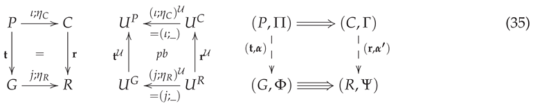
Any substitution represents a derived operation in a -structure as defined in (4). As discussed in Section 4.2.3, composition of substitutions in the category represents the composition of corresponding derived operations for any -structure , thus the commutative square of substitutions on the left in (35) transforms for any into the commutative square of derived operations in the middle of (35). Note, that the derived operations and are simple projections! We show that this commutative diagram of derived operations is, in analogy to (27), also a pullback in .
We have to prove that there is for any pair , of interpretations with a unique interpretation with and . The two uniqueness conditions enforce the following definition of
where the case is entailed by the definition of in (34) and the definition of derived operations in (4): That is, we have where is the unique extension of with thus for all the condition forces and, thus equivalently, for all .
It remains to show that for all . Due to the definition of in (36), we have thus the diagram below is commutative with an inclusion map and according to (17). In such a way, we get for any due to the assumption that .
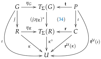
Analogously to Section 5.3, we extend the context to a -specification with constructed out of the -expressions in and . To achieve strictness of the resulting -specification implication, we simply declare . Keep in mind that the condition ensures for all according to Lemma 4.
To include the -expressions from , we have first to extend the substitution to a -indexed family of renaming substitutions. If , we can simply set since . Due to the definition of in (34), we get in this case. If , we can freely choose a set of fresh bound variables, i.e., with , thus there exists an isomorphism . Using the shorthand , we can summarize our definitions by .
Our definitions ensure, that the pair complies with the condition of a strict separation of free and bound variables, i.e., is indeed a -specification. We also get a strict -specification implication (see the right square in (35)). Moreover, the pair defines, by construction, a match thus Proposition 3 entails
In full analogy to Corollary 5, we can prove that the application of a -specification implication as a deduction rule via substitutions is semantically sound.
Proposition 4
(Specification Implications as Rules: Soundness). For any Σ-structure with , i.e., for , and any match it holds that , i.e., for .
Proof.
The strict -specification implication gives rise to the trivial renaming substitution , with for all thus the inclusion "⊆" is ensured by Proposition 3. It remains to show "⊇".
If , the inclusion trivially holds. If , we consider an arbitrary . Since is a match, we get , due to Proposition 3, thus there exists a with due to assumption .
In analogy to Section 5.3, we can also define a non-strict variant of rule application by simply defining instead of . A corresponding slight variation of the proof of Proposition 4 provides the following Corollary.
Corollary 7
(Non-strict Variant of Rule Application: Soundness). For any Σ-structure with , i.e., for , and any match it holds that , i.e., for .
Remark 24
(Non-proper Substitutions). In case that is anon-proper substitution, i.e., can be described as the composition of maps and , the definition in (34) of with entails that is also a non-proper substitution, i.e., can be factorized into with maps and . So, in this case, our construction of boils down to the construction of a pushout in of the span of maps representing the commutative diagram in the category depicted left in (35). In other words: There is no need to adapt Section 5.3 to Σ-specification implications since this adaptation simply is a special case of the constructions we presented in this subsection!
Remark 25
(Extension of Premises). What we will mainly need for our analysis of traditional deduction calculi is the extension of the premise of a given specification implication by new free variables and/or new expressions. To perform this simple task, we have to apply the given specification implication as a rule and, in some cases, it may be necessary to take additional measurements to enable rule application.
For a Σ-specification implication let be given an inclusion map and a Σ-specification . If the set is empty, no renaming of bound variables is necessary! is a legal Σ-specification and establishes a match in the sense of Definition 20, according to Remark 24.
In case , we chose a set V of fresh variables with together with a bijective map , and define a Π-indexed family of bijective renaming substitutions , with for all and if and if .
First, this ensures that is a match in the sense of Definition 20. Second, we can apply the rule , in a strict and non-strict way, via the match and it is ensured that we obtain legal Σ-specification implications and with , a bijection and .
Finally, entails and for any Σ-structure according to Corollary 7 and Proposition 4, respectively.
If , it still may happen that , thus the only simplification is that and that .
In contrast to the extension of contexts, the reduction of contexts doesn’t require any additional efforts. Be aware that this only works in the unsorted variant of first-order logic!
Corollary 8
(Reduction of Contexts). For any Σ-specification implication and any sets P, C of variables with , , we get a legal Σ-specification implication and for all Σ-structure
Proof.
The assumption , i.e., , implies . First, we have due to Corollary 6. Second, we obtain by (A23) and Corollary 6: , and thus , i.e., . □
We hopefully provided enough evidence that we can transform, by renaming of bound variables, any set of traditional first-order formulas into an equivalent -specification given by a set X of variables with and a set of -expressions on X, i.e., of traditional well-formed first-order formulas complying with Barendregt’s variable convention. Moreover, we can transform any pair of sets of traditional first-order formulas into a -specification implication , in the sense of Definition 18, with , , complying with the strong fresh variable condition .
After this is settled, we will assume in our analysis of traditional deduction calculi in the following two sections that those necessary transformations are tacitly done in the background. Moreover, we assume that the necessary renamings of bound variables for extensions of premises, as described in Remark 25, are also tacitly done.
7. Deduction in Traditional First-Order Logic
We investigate three different deduction calculi for traditional first-order logic - in this section a Hilbert System and a Gentzen’s system and, then, a Natural Deduction System in Section 8.
We are interested to analyze, understand and formalize, by means of the novel concepts context and specification implication, the structural essence of reasoning in each of the systems and, thus, the crucial conceptual differences as well as their commonalities. Especially, we are interested to formally grasp the different meanings and semantics of the turnstile symbol ⊢ and the inference line.
7.1. Hilbert System
We study the proof system for first-order logic presented in [4]. We learned from [33] that this system can still be seen as one of the very many Hilbert Systems and will, therefore, use the name instead of the name used in [4]. According to [4], the proof system is devised to define a relation with the set of all well-formed first-order formulas for a signature . It consists of
Axioms : Ā0: , for all ;
A1: ;
A2: ;
A3: ;
A4: if is legal ;
Rules :: MP: ;
∃I: if At first glance, it may look like that the elements in can be encoded as -specification implications. The relation is meant, however, to reflect the semantic entailment relation ⊩ between sets of formulas and single formulas. Note, that we use the symbol ⊩ for semantic entailment instead of the symbol ⊧, as it is quite common in the literature. We prefer to exclusively reserve the symbol ⊧ to denote the validity (satisfaction) relation between structures and formulas (of different kind).
means that implies for all -structures , where (or ) is valid for a -structure if (or A) becomes true for all (!) variable assignments in . The so-called universal closure (compare [4], p. 232 and [33], p. 372) transforms an open formula A into a closed formula and a set of open formulas into a set of closed formulas, respectively. We have (or ) if, and only if, (or ) thus can be equivalently expressed by the condition that implies for all -structures .
At the beginning of Section 5.2.2 we exemplified that -sketch implications (and thus also -specification implications) offer the novel device of unconditional -assertions to formally grasp the traditional definition of the satisfaction relation ⊧ (also applicable for formalisms lacking a universal quantification operator!). We can utilize the satisfaction of -specification implications in -structures, due to Definition 18, and reformulate that if, and only if, implies for all -structures . Remind, that means nothing but . So, in view of LoSiCs the turnstile symbol represents implications between -specification implications of the form with and -specification implications of the form with . For convenience, we will mostly write instead of . We provide evidence that this fresh and novel view on system is consistent with the traditional view by re-validating the soundness of system in terms of specification implications.
7.1.0.1. Axiom A0
This is the only axiom schemata or rule where is relevant! For any -structure we assume with . By definition, we have and thus . Since the composition of -specification implications preserves satisfaction, we can conclude and thus also , due to Corollary 8.
Obviously, the -specification implication is the essence of this axiom. It will re-emerge as an axiom in the Gentzen System .
7.1.0.2. Axioms A1 - A3
All three axiom schemata are independent of ! One can argue that these axiom schemata can be directly inherited from propositional logic. As already discussed at the beginning of Section 6 this argumentation may be not convincing for everyone since it is not clear in what sense open formulas in the traditional approach represent propositions.
As alternative, we can validate these axiom schemata by Boolean Algebra reasoning. We exemplify this for Axiom A1. With we obtain, due to Definition 7:
and thus as required.
7.1.0.3. Axiom A4
To turn "" into a legal -specification, we require and, instead of " is legal", that . This can be achieved by an appropriate renaming of bound variables. To allow , we rename , in addition, the bound variable x in by a fresh variable z with . That is, we replace by . Also this axiom schemata is independent of . For all -structures we show that with where due to (1) and due to (33).
We don’t work with substitutions of a single variable by a single term but only with maps from sets of variables into sets of -terms. To grasp the situation in Axiom A4, we also consider the set of variables. We define a substitution with and for all . We obtain , according to Definition 11, and for the inclusion map .
We must show for any , i.e., that implies . According to (3), the substitution defines a derived operation with . We have if, and only if, , due to (20), and we get and thus by the semantics of existential quantification in Definition 7.
7.1.0.4. Rule MP
Rules in System introduce a third level of implications since inference lines in System establish implications between implications relating -specification implications. Such a kind of twofold nesting of implications looks indeed a bit "unnatural".
Rule MP is, however, independent of thus the validation of the rule means to show for any -structure that and implies where . This can be easily done.
and means and thus we also get , i.e., . Relying on the semantics of implications in Definition 7, we can easily show by Boolean Algebra reasoning:
Since composition of -specification implications preserves satisfaction, we can finally conclude as desired.
The -specification implication is the essence of this rule and will re-emerge as a rule in the Natural Deduction System .
7.1.0.5. Rule ∃I
Also this rule is independent of thus it suffices to show for any -structure that implies with , and thus since .
We consider the inclusion map and turn the soundness proof by contraposition for Rule ∃I in [4], p. 261 into a direct proof of the following lemma.
Lemma 5
(Rule ∃I: Sem.). for all Σ-structures if .
Proof.
Due to the definition of universal operators in (A21), we have to show for any that for all with . entails thus we get by assumption . Due to Lemma 3, this implies thus we have shown , as required. □
Finally, we assume , i.e., . By Lemma 5, Corollary 6 and equation (29) we obtain , i.e., , thus Rule ∃I is indeed validated.
7.2. Gentzen’s System
There are many variants of System around. At the end, we decided against the variants presenting Sequent Calculi by a set of rules cleanly devided in left rules and right rules [34]. We decided to rather rely on [32] instead, since the strong relation between System and Natural Deduction is coherently addressed and explained in [32]. After a Natural Deduction calculus is presented and discussed in [32], the authors write:
This is the classical formulation of the calculus of natural deduction. To prepare the things we want to do later (and to get around the somewhat un-licensed extension by hypothetical reasoning in the calculus), we will reformulate the calculus by lifting it to the “judgements level”. Instead of postulating rules that make statements about the validity of propositions, we postulate rules that make statements about derivability. This move allows us to make the respective local hypotheses in Natural Deduction derivations into syntactic parts of the objects (we call them “sequents”) manipulated by the inference rules.
We like this didactical approach very much, but will, nevertheless, first discuss System and only afterwards Natural Deduction. Our didactical reason is that we want to emphasize the stepwise reduction of "nesting levels" of implications. The second, more practical, reason is, that we must develop another chunk of theory to formally grasp and finally license hypothetical reasoning. We will only introduce and elaborate the necessary novel concept of open specification implications in Section 8.
Moving from System to System , we get rid of one level of nesting of implications! Sequents in System are nothing but -specification implications of the form with thus the inference lines in System represent implications between a finite set of -specification implications of this form and a single -specification implication of this form. We present first the propositional rules of System according to [32] where we use the symbols "→", "⊥" instead of the symbols "⇒", "F" in [32]. To safe space, we will also simply write ⊢ instead of .
*6ex Axiom weaken TND
For the remaining part of this subsection let be an arbitrary -structure. We discuss the first two rules. The rule Axiom corresponds to Axiom A0 in System and that with has been already shown in Section 7.1. Analogously, we can argue that with , i.e., , entails , i.e., , thus also rule weaken is validated.
Relying on Remark 25 and the fact that the validity of -specification implications is closed under composition, each propositional rule, where all involved sequents share the same antecedent, can be validated by proving that a certain single underlying essential Σ-specification implication is valid in any -structure . These essential -specification implications appear later as rules in the Natural Deduction System ! We list all those rules together with the corresponding essential -specification implication.
We validate rule TND. We do have for the essential implication, due to the semantics of disjunction, and thus for by Remark 25. trivially holds since thus we obtain by composition of -specification implications.
Rule corresponds to rule MP in System . In Section 7.1 we have already shown for the essential implication thus we have also for by Remark 25. and trivially imply , i.e., , thus we finally obtain by composition of -specification implications.
All the other essential -specification implications in the above listing are valid in any -structure according to the semantics of Boolean connectives, thus the corresponding rules can easily be validated analogously to the rules we explicitly validated.
It remains to validate the three rules where the involved sequents don’t share the same antecedent. For rule we set . means thus we obtain and, equivalently, , i.e., .
For rule we set . The assumption , i.e., , implies and thus since by assumption , i.e., , and , i.e., . This proves .
To validate rule we need to prove the following semantic deduction theorem for specification implications with .
Lemma 6.
iff
Proof.
"⇒": , i.e., entails, according to the semantics of the connective →, , i.e., .
"⇐": , i.e., , implies , i.e., . □
After the propositional rules we now examine the four quantifier rules of System .
*2ex is legal is legal
c a new Skolem constant
We postpone the validation of rule to Section 8. In contrast to rule , the two rules and can be validated by proving the soundness of a corresponding underlying essential -specification implication which re-emerges later as a rule in the Natural Deduction System .
Rule is the sequent variant of Axiom A4 in System . We adapt the argumentation in paragraph Axiom A4 on page 39: To turn the sequent into a legal -specification implication with , we require and , instead of " is legal". This can be achieved by an appropriate renaming of bound variables.
To allow , we rename , in addition, the bound variable x in by a fresh variable z with and . That is, we replace by . where , due to (1), and with for any -structure , due to (33).
We show that implies for any -structure . has been proven in Section 7.1, thus we obtain, by Lemma 6, for the essential -specification implication underlying rule . is ensured by Remark 25, thus we finally get , as desired, since validity of -specification implications is preserved by composition.
Rule can be validated analogously to rule . To turn the sequent into a legal -specification implication with , we impose the same restrictions as for rule "", and we correspondingly replace by to allow where and with for any -structure .
We want to show that implies for any -structure . This can be done by proving for the essential -specification implication underlying rule . Analogously to the case of Axiom A4 on page 39, we consider the set of variables and define a substitution with and for all , thus we have and for the inclusion map . Applying the derived operation to any , we get given by , due to (3), and thus . This entails due to the semantics of universal quantification. According to (20), means, however, nothing but , as required.
implies , due to Remark 25, thus is indeed entailed by since composition of -specification implications preserves validity.
In case of rule , we choose and turn the sequents and into -specification implications and , respectively.
For , we have for any -structure since , due to Definition 7, for the proper inclusion map . That is, this implication simply represents the semantics of existential quantification.
"c a new Skolem constant" means, especially, and thus we can utilize c to describe the pushout of the span of inclusion maps and the corresponding extension of the context I of the -specification via the inclusion map (compare Section 6.4 and, especially, Remarks 24 and 25).

Corollary 7 ensures thus entails by composition of -specification implications. So, for each there exists an such that and therefore, due to Corollary 6, also as well as . In such a way, we get . So, if , we also have by composition of -specification implications. It remains to get rid of the "new Skolem constant c".
We use the same trick as in the validation of Rule ∃I in System . is a legal -specification and we can factorize into . if, and only if, . By Corollary 6 and equation (29), we obtain and thus . If desired, we can even conclude , due to Corollary 8.
Remark 26
(Gentzen’s System ). Gentzen’s System [34] and its variant System in [4] work with sequents where both Γ and Δ are finite sets of formulas. Those sequents correspond to implications of the form .
Until now, we considered only "conjunctive Σ-specifications" with a semantics given by intersection for any Σ-structure . To treat sequents within the LoSiC-approach, we must, however, also introduce "disjunctive Σ-specifications" with semantics given by union . Then, we can formalize sequents as Σ-specification implications with if, and only if, for the inclusion map . Note, that since distributes over arbitrary unions!
We are convinced that deduction systems like and can be validated by means of Boolean Algebra reasoning analogously to System . Due to limited time, space as well as motivation on our side, we postpone a detailed exploration of those systems to another occasion.
8. Natural Deduction and Open Specification Implications
Moving from System to the Natural Deduction System , we finally reduce the level of nesting of implications to one for all rules where we have been able to identify an essential underlying -specification implication. In System these essential implications are simply represented as rules, i.e., the horizontal implication arrows "⟹" are transformed into vertical interference lines. In other words, we simply delete the "same antecedent" in the corresponding rules in System to obtain a rule in System . The reader may forgive us for not repeating those rules in their corresponding -shape.
Attention, in case of rule we also delete both , but the condition "" transforms into the somehow puzzling condition "A does not depend on any hypothesis in which x is free" in (49).
In the remaining four rules we also drop in all the antecedents thus the conclusions of the four rules become plain -expressions. The premises of the rules remain, however, with a kind of implicational residue. The problem is to describe this implicational residue in a, more or less, precise way! The three propositional rules , , in System are presented in [32] as follows:

As the rules may be nested, both the rules and the corresponding assumptions are decorated with a marker (here the number 1). We will discuss one nested proof in Section 8.4.
The semi-formal notation "" is usually read as "there is a proof showing that B holds under the additional hypothesis that A holds". Turning upside down the argumentation in [32], cited at the beginning of Section 7.2, we pose the question if it is possible to describe the result of such a hypothetical proof "" in a precise formal way and independent of the concrete proof. The answer is that we can indeed do this by introducing the concept of open specification implication. We will define, elaborate and apply this novel concept in the remaining part of this section.
8.1. Open Specification Implications
We combine two lines of observations and insights. First, we observe that assertions of the form "we can prove B under the additional hypothesis that A holds" are widely used as so-called universal properties to define concepts and to formalize findings in Category Theory. Second, the LoSiC-approach is based on the insight that the difference between closed formulas and open formulas essentially boils down to the difference between empty contexts and non-empty contexts, respectively. Statements in context are statements about single interpretations of contexts in a -structure . For the empty context there is, however, only exactly one interpretation in a -structure , thus a statement in the empty contexts turns into a statement about the -structure as a whole!
According to Definition 18, specification implications can serve as another tool to formulate assertions about -structures as a whole and correspond, in this sense, to closed formulas. In analogy to -expressions, we simply propose to equip specification implications with a potentially non-empty interfaces.
Definition 21
(Open Specification Implication: Syntax). Anopen -specification implication is given by a Σ-specification implication , in the sense of Definition 18, and aninterface.
In analogy to -expressions, we can also define a semantics for open specification implications in any structure.
Definition 22
(Open Specification Implication: Semantics). For a Σ-structure the semantics of an open Σ-specification implication in is defined as follows: For all it holds that if, and only if, for the inclusion maps and , i.e., if, and only if, for all extensions of along satisfying Π there exists an extension along satisfying Δ.
We can also equivalently reformulate Definition 22 in a more compact way
In case , i.e., , we do have only one assignment . Since , we indeed reconstruct the validity condition for -specification implications in Definition 18 (compare also (25)):
In case , we immediately obtain the following corollary.
Corollary 9
(Open Specification Implication: Semantics). For all Σ-structures it holds that
- 1.
- and thus
- 2.
- and
- 3.
- .
In addition to Corollary 9.3, we can also prove a semantic deduction theorem for open specification implications by slightly adapting the proof of Lemma 6.
Lemma 7.
The declaration "" for open -specification implications has the same purpose as the declaration "" for -expressions. It declares the set of variables that are considered to be the potentially available free variables in . The set of free variables, actually appearing in , is the set while the set of all bound variables is . Note, that, due to Definition 22, the variables in are implicitly universal quantified while the variables in are implicitly existential quantified!
We propose to formalize assertions of the form "" as open -specification implications thus the premises in the rules , , in (40) become -specifications enriched by open -specification implications as a new kind of statements in context.
In the traditional lazy approach all bindings are implicitly given by inclusion maps. So, if is an element of for an enriched -specification , we must have and, analogously to definition of the semantics of -expressions in (12), we define for a -structure the semantics of the open -specification implications in context G by
for the inclusion map . The semantics of an enriched -specification is defined analogously to (28) thus we also obtain a corresponding variant of Corollary 6 for enriched -specifications.
To approve our proposal two things should be at place. First, we must clarify what role open -specification implications in enriched -specifications play in deduction. Second, it is necessary to demonstrate that open -specification implications enable us indeed to formally grasp the results of hypothetical reasoning.
What is our view on a single process of deduction? We start with a set of hypotheses given by an ordinary -specification . Than we successively extend this initial -specification by applying the available deduction rules in a strict way. Following our proposal, we will also generate enriched -specifications. In such a way, each stage of an actual deduction process gives rise to a strict -specification implication from the initial ordinary -specification to the present enriched -specification . Note, that especially contains all the "hypotheses in which x is free" mentioned in the condition for the -version of rule in (49)!
An open -specification implication in an enriched -specification is nothing but a deduction rule in waiting position locally bound to the context G by the inclusion map . Once we are able to extend the binding to a match for a map with , we can apply the -specification implication as a strict deduction rule as described in Section 6.4 (compare especially Remark 24).
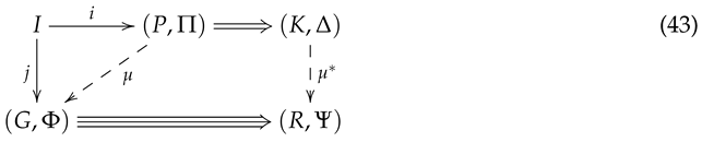
We shortly discuss the soundness of such a deduction step. For any -structure we do have since is an element of . Due to Proposition 3 and Definition 22, this ensures for any . Slightly varying the proof of Proposition 4, we can show, in such a way, that .
8.2. Licensing Hypothetical Reasoning
We evidence that open -specification implications are indeed an appropriate tool to formally describe and finally license hypothetical reasoning. Especially, we demonstrate that the effect of hypothetical reasoning can be described by adding locally bound open -specification implications to the present enriched -specification representing the actual status of all the things that have been deduced and/or introduced during a concrete deduction process.
How to transform a semi-formal notation like "" into an open -specification implication ? "A" is transformed into and "B" into . The appropriate choice of the sets I, P, K of variables depends on the concrete situation but, at least, we should have the following inclusions , , in addition to the inclusions . The inclusion map describes to what part of G the open -specification implication will be bound. The result of a sound hypothetical reasoning step can be only grasp by adding to if for all -structures the following soundness condition is satisfied:
What means the step from "A" to "", i.e., the introduction of A as a fresh hypothesis? In LoSiC-terms it means to apply, in a strict manner, the -specification implication via the trivial match as described in Section 6.4 (see the right diagram in (45)). In other words, we add the hypothesis to ! Keep in mind, that and that the underlying pushout of maps in the left diagram in (45) replaces the variables in by entirely fresh variables in , referred to as new Skolem constants in [32], via a bijective map .

In some texts like [35], using the Fitch style to present proofs by natural deduction, the step from "A" to "" is accompanied by writing a note like "want B". Correspondingly, we may mimic this step by also drawing the arrow "" in (45).
In the next modus "", we extend by successively applying, in a strict manner, sound general deduction rules or locally bound deduction rules in waiting position from . In such a way, we have at any stage of extension. The objective is to finally deduce an enriched -specification such that there exists a match with for the underlying maps. Note, that such a match provides for all the implicitly existentially quantified variables in corresponding witnesses in H!
In case of success, we reach the stage "" and the "auxiliary deduction" (called "subproof" in [35]) has served its purpose. What is called discharging the assumptions of that subproof in [35], p. 108, can be formalized by adding to and replacing the right diagram in (45) by the strict -specification implication
This final step of discharging is semantically sound if, and only if, the condition in (44) is satisfied. The following proposition shows that this is indeed the case.
Proposition 5
(Hypothetical Reasoning: Soundness). Let the Σ-specification implication in (45) be strict and valid in the Σ-structure , i.e., we assume . Then we do have for any match , with for the underlying maps, that , i.e., for all .
Proof.
We assume . If , we trivially have, due to Definition 22, that . If , let be arbitrary thus we especially have . Due to the pushout in (45), there is a unique with and . The assumptions , entail , and thus .
Since , there exists a with and while the assumption ensures . This finally proves , as required by Definition 22, since . □
8.3. Validating Hypothetical Reasoning Rules
Backed up by Proposition 5, each of the rules , , in (40) can be transformed into a semantically equivalent implication from an enriched -specification into an ordinary -specification given by a single -expression. In such a way, the validation of the three rules can be done by validating these corresponding enriched essential implications.
For rule the diagrams in (45) specialize with to

thus the rule transforms into the implication . By Corollary 9.3 we do have for all -structures . This proves the soundness of the rule!
For rule we need two independent auxiliary deductions as in (47), that can be performed in any order (or maybe even in parallel), resulting in an enriched -specification with and .
In such a way, the rule transforms into the implication . Due to Corollary 9.1 and the semantics of negation we obtain by some Boolean Algebra reasoning for all -structures thus the rule is validated.
By two independent auxiliary deductions as in (47) rule transforms into the implication with where . Due to Corollary 9.1, we obtain by some Boolean Algebra reasoning for any -structure
and thus as required.
Next we analyze the quantifier rule in System as presented in [32]
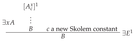
In this case, we get a non-trivial instance of (45). We set , and . As already seen in (39), the new Skolem constant c can be utilized to construct the necessary pushout of inclusion maps, i.e., we can set and .

A corresponding auxiliary deduction transforms the rule into the implication with . We show , i.e., , for any -structure . Let be . We have thus implies that there exists a with and, in such a way, also . On the other hand, means, according to Definition 22, that . Therefore, there exists a with . This finally proves as required.
Attention! Due to the commutativity requirement , the match translates the variable x into the Skolem constant c! We do not know if it is a flaw of the LoSiC-approach, that we actually require "", or if this is simply overseen in [32]? In [35], p. 119, it is explicitly required that "the constant c must not appear in , in B, or in any undischarged assumption". So, at least compared to [35], the LoSiC-approach to hypothetical reasoning seems to be a bit more flexible since we allow that c appears in B. Keep in mind, that we can replace by the semantically equivalent formula as we did it for the validation of Axiom A4 in System , for example.
To deliver on our promise from Section 7.2, we finally validate rule .

* means that A does not depend on any hypothesis in which x is free.
The informal version Intuition of rule indicates how we can validate rule by means of Proposition 5. For the -version of the rule we set and . Condition ensures that as well as are -specifications where we have , due to Corollary 6, for the inclusion map and any -structure . We show that implies .
Let us assume , i.e., . This gives rise to the following instance of (45) with ,

Proposition 5 entails thus we get for any also and, in such a way, . According to Definition 22 this is equivalent to . This gives us the inclusion .
Applying to both sides of the inclusion as well as utilizing (29) and the semantics of universal quantification we arrive at . This finally entails , as required, due to Corollary A4 and Lemma 3.
The -version of rule can be analogously validated by simply replacing by . While is supposed to only contain -expressions (formulas), we allow that also contains open specification implications and that those locally bound deduction rules in waiting position can be applied, in the spirit of (43), to arrive at !
8.4. Nested Hypothetical Reasoning
To illustrate the LoSiC-approach to deduction, we discuss the deduction of the -specification implication with (compare axiom A1 in Section 7.1). We will go step by step through the corresponding proof in System visualized by a proof tree and in Fetch notation as follows:
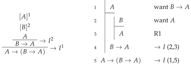
First, we introduce the two hypotheses and reach in System the stage

Also representing the two want-phrases, we obtain in the LoSiC-approach the diagram
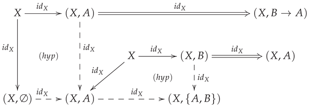
In the next stage
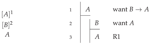
we realize that we do have the "wanted A" available and get the diagram
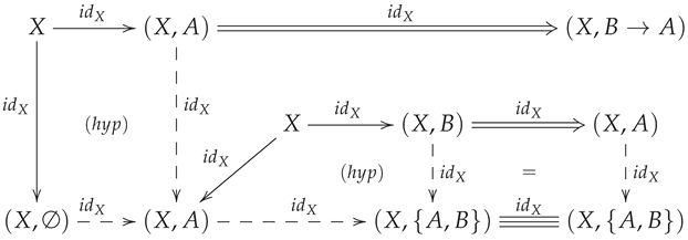
Closing the subproof and discharging the assumption gives us in System
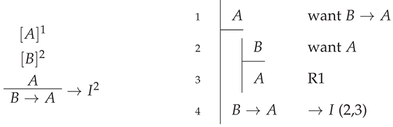
In the LoSiC-approach, we close the subproof and discharge the assumption by turning into the enriched -specification . Due to Proposition 5, we proved, in such a way, the enriched -specification implication . Fortunately, Corollary 9 allows us to use instead the equivalent pure -specification implication .
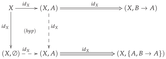
Finally, we do have the "wanted ". We can close the whole proof and also discharge the assumption . In view of LoSiCs, we deduce the enriched -specification under the assumption , thus we have finally proved the pure -specification implication according to Proposition 5 and Corollary 9.
9. Conclusions and Further Work
We accomplished the first of the projects envisaged in the concluding section of [17]. We developed a conservative extension of the traditional institution of unsorted first-order logic to an unsorted first-order Logic of Statements in Context, comprising not only "closed" but also "open formulas". A crucial novelty, compared to [17], is that we in detail worked out an appropriate variant of a hom-set based semantic calculus of quantification and consequently used this calculus in our analysis of deduction in first-order logic.
We showed that the traditional presentation of first-order logic, where neither variable declarations nor contexts are explicitly considered, is equivalent to a first-order Logic of Statements in Context where all bindings of formulas to contexts and all morphisms between contexts are restricted to (implicit) inclusion maps.
By a kind of "methodological accident" this equivalence reinvents, however, Barendregt’s variable convention [18]. So, from a more technical point of view, we had to find out how to integrate Barendregt’s variable convention into traditional first-order logic in a syntactic and semantical correct way. It is maybe worth to mention that Barendregt’s variable convention allowed us to introduce renaming substitutions executing substitutions of free variables by terms and renamings of bound variables in parallel.
Relying on this preparatory efforts, we succeeded in exhaustively analyzing, formalizing and validating three of the basic kinds of deduction calculi for traditional first-order logic by means of the LoSiC-concepts context and specification implication, namely a Hilbert System and a Gentzen’s system and a Natural Deduction System .
The crucial innovation of the paper is the introduction of open specification implications and the related idea of deduction rules in waiting position. This innovation enabled us to syntactically represent the outcome of hypothetical proofs in a precise formal way and independent of the concrete hypothetical proof. In such a way, we have been able to finally license hypothetical reasoning in a proper syntactic and a semantical sound way.
To extend, consolidate and further develop the open framework of Logics of Statements in Context, we propose four projects:
- Open Injectivity
-
Following [30,31], we decided to replace the term "Horn Logics", used in [17], by open injectivity. Open specification implications, introduced in this paper, are a first example of open injectivity. Obviously one could iterate the definition of open specification implications. We are, however, not sure that there really is a reason and/or need to do this at the moment. On the other side, nested open injectivity can only unfold its full potential in the presence of explicit variable declarations and contexts. This full potential is needed to describe and formalize reasoning in Category Theory, for example.Since Category Theory relies on universal properties, there is no need for first-order formulas. Instead, one can use nested open sketch implications based on relational atoms to formalize Category Theory (compare [10]). Therefore, we decided to elaborate in the next paper a full account of this kind of nested open injectivity for arbitrary Logics of Statements in Context with Category Theory as running example. Note, that the habit of "want phrases" in the Fitch notation for Natural Deduction is strongly related to the heuristics of "diagram chasing" in Category Theory!
- LoSiC-Deduction in the Unsorted Case
- Writing this paper, we finally realized that our initial idea to simply borrow deduction calculi from traditional first-order logic was by far too naive. We also learned that substitutions should be used as morphisms between contexts. To also have in this case Institutions of Statements in Context at hand, we have, however, also to allow substitutions as bindings! What has to be done is to upgrade the Institutions of Statements in Context in the present paper to institutions with substitutions as bindings as well as context morphisms. Based on this, the necessary bigger effort should be spend to adapt, at least, one of the traditional deduction calculi to the corresponding upgraded first-order Logics of Statements in Context. We are convinced that Gentzen’s system and its twin Natural Deduction are reasonable candidates to get this job done.
- Traditional Deduction in the Many-Sorted Case
- Another bigger project would be to extend the ideas, constructions and findings of the present paper to traditional many-sorted first-order logic. The remarks concerning the many-sorted case, scattered over the paper, together with [17] should establish a reasonable starting point to attack such a project. In a nutshell, the crucial problem with many-sortedness is that we can not get rid of variables in for a -specification by simply deleting them! That is, assertions as in (29) and Corollary 8, for example, vanish in the many-sorted case. The only chance to get rid of a variable , in a sound way, is to find a -term t over (compare rule "Concretion" in [36]). Note, that the concept of context enables us to address and potentially deal with this issue without utilizing the crutch of universal quantification as it is done in [36].
- Gentzen’s System
We will retire in autumn 2026 but will continue with our research. Everyone is invited to work on the last three projects - alone or in cooperation with us.
Funding
This research received no external funding.
Acknowledgments
This paper would not have seen the light of day without the intense and creative exchange of ideas with Nicolas Behr in Spring 2025. I am also very thankful to my colleague Michał Walicki and Phd-student James Hobson for all the inspiring and supporting discussions during a seminar on this topic at the University of Bergen in autumn 2025.
Conflicts of Interest
The author declares no conflicts of interest.
Appendix A. Operators on Predicates
More than two decades ago we learned from [37] that the semantic effects of existential and universal quantification can be characterized as left and right adjoints, respectively, of projection maps. That time, we ignored this insight as too abstract for our own research.
During an intense discussion with Nicolas Behr in spring 2025 we learned, however, that this insight is quite relevant for understanding, presenting and validating LoSiCs. Therefore, we present here the basic definitions, constructions and results concerning hom-set predicates for the special case of the category and in the specificity, we utilize them in this paper. That one can define hom-set predicates and a corresponding calculus in arbitrary categories is quite obvious as the interested reader may check [38,39].
Appendix A.1. Shift, Existential and Universal Operators for Maps
For any set A the powerset construction gives us a partial order and a respective Boolean Algebra at hand, where is the compliment of . It is quite common to call a subset a "property" of elements in A or a "predicate" for A. Keep in mind that any partial order can equivalently be seen as a partial order category, i.e., a category with at most one morphism between two objects and with identities the only isomorphisms.
For any map the formation of pre-images
defines a monotone function (a functor) from into
For historical reasons [38,39,40] we call this function the shift operator given by f. The reader may think about a "shift of perspective" from B to A by returning to A along .
Dually, the formation of images defines for any map a monotone function (a functor) from into defined for all by
As one can observe, the formation of images is related to existential quantification in the sense that contains exactly all those elements from B for which there exists a pre-image w.r.t. f ( a "witness/antecedent") in M. Therefore, we call this function the existential operator given by f and adapt from [38,39] the notation
The first crucial observation is that the operators and establish a monotone Galois Connection (an adjunction) between the partial orders (categories) and .
Corollary A1
(Existential Galois Connection 1). For any and we have
- unit:
- counit:
- adjunction:
- iff
Note, that is called "left" adjoint to (and, correspondingly, "right" adjoint to ), in symbols, since appears in the adjunction statement on left of the "arrow" ⊆ while appears on the right!
For all we do have . is surjective if, and only if, thus surjective implies for all . The other way around, if there exists only a map if also thus we have which is trivially surjective. If , the condition implies for all singletons that , thus we get the following characterization of surjectivity:
Obviously, is injective if, and only if, is either a singleton or empty for all . means that . This is the case for all if is injective thus we have the following implication:
The second, more striking observation is that universal quantification is dual to existential quantification in a rigorous categorical sense. Universal quantification turns out to be nothing but the right adjoint to the shift operator.
For any map we can define a monotone function (a functor)
called the the universal operator given by f and defined for all by
formalizes universal quantification in the sense that contains exactly all those elements from B for which all (!) pre-images w.r.t. f are in M. Be aware, that we always have since for all .
We get indeed a monotone Galois Connection (an adjunction) between the partial orders (categories) and .
Corollary A2
(Universal Galois Connection 1). For any and we have
- unit:
- counit:
- adjunction:
- iff
The interplay of the Universal and the Existential Galois Connection gives us a simple, but useful, Corollary at hand.
Corollary A3
(Shift vs Existential and Universal). For any map and all , it holds that and implies .
For all we do have thus surjective, i.e., , implies for all . The other way around, the condition for implies . In such a way, we get another characterization of surjectivity in terms of universal operators and, thus, an overlapping of existential and universal quantification due to (A5):
For all we do have iff iff . This means that we do have another overlapping of existential and universal quantification:
thus injective also implies according to (A6).
Due to Corollary A2, the monotone function (the functor) is left adjoint to the monotone function (the functor) , in symbols. We can summarize the basic findings of this section by the following diagram.

Fortunately, the construction of shift, existential and universal operators is compatible with composition. For any maps and we do have
The first two equations are ensured by the fact that both constructions - the formation of pre-images and the formation of images - define functors from into , namely a contravariant and a covariant powerset functor, respectively. The third equation can also be shown straightforwardly.
We should mention that and as right adjoints distributes over arbitrary products, i.e., intersections, while and as left adjoints distribute over arbitrary sums, i.e. unions! Moreover, is compatible with respect to complements, i.e., for any map we have
since distributes over arbitrary unions, preserves disjointness and we consider only total maps.
Attention! As usual, the direction of "arrows" is a matter of tradition, taste, ideology and/or methodology. We work here with inclusions in accordance with the direction of the corresponding inclusion maps . In [38,39] they also use inclusions ⊆ but denote them by ⊧ even if the direction of logic entailment would rather indicate ⊇! Note, that the sequence of adjunctions matches the well-known sequence of adjunctions characterizing the four basic constructions sum-copy-product-exponent in mathematics and category theory.
Appendix A.2. Shift, Existential and Universal Operators for Pre-composition Maps
This special kind of maps for arbitrary categories is addressed in [38,39]. Here we consider this special kind of maps for the category .
To ease accessibility of the paper, we instantiate definitions, constructions and results in Appendix A.1 for hom-sets and pre-composition maps induced by maps and defined for any set U, by
In LoSiCs, U varies over all potential carriers of structures, i.e., we assume U to be a non-empty set since in this paper!
As exponents we use sets of variables or contexts while . Elements in are also called (variable) assignments and elements in interpretations. In our analysis of traditional first-order induction calculi, we mainly meet inclusion maps while is usually callled a projection. Nevertheless, we consider in this section arbitrary maps .
In contrast to [38,39], we focus in LoSiCs on "syntactically represented" (hom-set) predicates. Any syntactic entity, like a -expression, a -statement in context or a finite -sketch represents for each (!) -structure a corresponding predicate in . Different -structures can, however, share the same carrier! So, in case we have to define (hom-set) predicates over K in the spirit of [38,39], we could consider -indexed families of subsets instead of -indexed families.
We adapt the notation in Appendix A.1 to the special case of pre-composition maps. First, we don’t use the identifiers of pre-composition maps but the identifiers of the underlying maps as subscripts for operators. Be aware that this reverses the direction of maps and thus the order of composition: For any maps , and any carrier U we have the pre-composition maps , where
Second, we use identifiers U of carriers as superscripts for operators.
For any map and any carrier U the formation of pre-images for the corresponding pre-composition map
defines a monotone function (a functor)
which we call the shift operator for U induced by ψ. In case of an inclusion of sets of variables, is exactly the set of all extensions of the variable assignment to Y.
Dually, the formation of images defines a monotone function (a functor)
called the existential operator for U induced by ψ and defined for all by
We instantiate the adjunction from Corollary A1 for pre-composition maps.
Corollary A4
(Existential Galois Connection 2). For any and
- unit:
- counit:
- adjunction:
- iff
Note, that is called "left" adjoint to (and, correspondingly, "right" adjoint to ), in symbols, since appears in the adjunction statement on left of the "arrow" ⊆ while appears on the right!
For any map and any carrier U we obtain a monotone function (a functor)
called the the universal operator for U induced by ψ and defined for all by
Be aware, that we always have since for all .
We instantiate the adjunction from Corollary A2 for pre-composition maps.
Corollary A5
(Universal Galois Connection 2). For any and
- unit:
- counit:
- adjunction:
- iff
Due to Corollary A5, the monotone function (the functor) is left adjoint to the monotone function (the functor) , in symbols. We can summarize the basic statements of this section by the following diagram with U an arbitrary non-empty set.

For pre-composition maps the compositionality statements in (A12) are transformed as follows. Keep in mind (A15). For any maps , and any carrier U we do have the following equations:
We round this section with a systematic analysis of surjectivity and injectivity of pre-composition maps. Since we only allow non-empty carriers U, all the hom-sets are non-empty for arbitrary K! By (A9), we do have for any map and any carrier U:
For we have and is surjective for the only injective map since for all .
For the pre-composition map is surjective for any carrier U if is injective, since all (!) injective maps with are split monomorphisms (sections) in , i.e., there exists a map such that . For any we obtain for thus is indeed surjective. Note, that we actually argue , i.e., is a split epimorphism (retraction) in for any carrier U.
In this paper we have thus we can choose . The split monic requirement "there exists a map such that " is equivalent to the requirement that is non-empty which is ensured if is surjective. In such a way we get the following equivalence completing (A24).
Deduction calculi in traditional unsorted first-order logic utilize inclusion maps and rely heavily on the equivalences in (A24) and (A25)!
surjective entails that is injective for all carriers U since surjective maps are exactly the epimorphisms in . In such a way, we obtain from (A6) and (A26) for all carriers U:
Remark A1
(Many-sortedness: Operators). There are two related reasons that the "lazy approach" to deduction in unsorted first-order logic does not work for many-sorted first-order logic.
Let S be a set of sort symbols with cardinality . First, for any S-sets , the condition , with the initial object in the category of S-sets and S-maps, doesn’t ensure that the set of all S-maps from K into U is non-empty. becomes empty if there is an with but !
Second, the condition doesn’t ensure that every injective S-map is split monic. is not split monic if there is an with but !
We can repair the equivalence in (A25) by replacing "injective" by "split monic", but we have to overcome our laziness anyway and must work with explicit variable declarations since the projections for are not anymore surjective by default!
Appendix A.3. Shift, Existential and Universal Operators for Substitutions
As shown in Section 3.3 any -substitution (declaration) defines a derived operation in every -structure (in the opposite direction).
To ease accessibility of the paper, we instantiate definitions, constructions and results in Appendix A.1 for the special hom-sets , i.e., sets of variable assignments, and derived operation represented by -substitutions . Note, that there is a certain small overlap with Appendix A.2 since every map can be equivalently represented by the -substitution .
We adapt the notation in Appendix A.1 to the special case of derived operations analogously to the adaptations in Appendix A.2. First, we use the identifiers of -substitutions as subscripts for operators. Be aware that this again reverses the direction of maps and thus the order of composition. Second, we must use identifiers of -structures, instead of identifiers U of carriers as in Appendix A.2, as superscripts for operators.
In Section 4.2.1 we discussed that any -substitution (declaration) can be extended to a map with where describes the application of the -substitution to all -terms over X! This enabled us to define the composition of two -substitutions , as the -substitution . Moreover, (18) shows that this composition of -substitutions reflects the composition of the corresponding derived operations ,
For any -substitution and any -structure the formation of pre-images for the corresponding derived operation
defines a functor, called the shift operator for induced by ,
Dually, the formation of images defines a functor
called the existential operator for induced by and defined for all by
We instantiate the adjunction from Corollary A1 for derived operations.
Corollary A6
(Existential Galois Connection 3). For any and
- unit:
- counit:
- adjunction:
- iff
By Corollary A6 the functor is left adjoint to , in symbols. For any -substitution and any -structure we obtain a functor
called the the universal operator for induced by and defined for all by
We instantiate the adjunction from Corollary A2 for derived operations.
Corollary A7
(Universal Galois Connection 3). For any and
- unit:
- counit:
- adjunction:
- iff
Due to Corollary A7, the functor is left adjoint to the monotone function (the functor) , in symbols. We can summarize the basic statements of this section by the following diagram with an arbitrary -structure .

For -substitutions the compositionality statements in (A12) are transformed as follows. Keep in mind (A28). For any -substitutions , and any -structure we do have the following equations:
Properties of derived operations can heardly be traced back to properties of the -substitution since the properties of heavily depend on the special properties of the operations in . Therefore, the findings concerning surjectivity and injectivity in Appendix A.1 for arbitrary maps can not be refined for derived operations.
References
- Wolter, U. Logics of Statements in Context - Category Independent Basics. Mathematics 2022, 10. [Google Scholar] [CrossRef]
- Chang, C.C.; Keisler, H.J. Model Theory; Studies in Logic and the Foundations of Mathematics; Elsevier Science, 1990. [Google Scholar]
- van Dalen, D. Logic and Structure. In Universitext, 5 ed.; Springer, 2013. [Google Scholar] [CrossRef]
- Walicki, M. Introduction to Mathematical Logic, extended ed.; World Scientific, 2017. [Google Scholar]
- Wechler, Wolfgang. Universal Algebra for Computer Scientists. In Proceedings of the Monographs in Theoretical Computer Science. An EATCS Series.; Springer-Verlag, Berlin Heidelberg, 1992; Vol. 25, p. 339. [Google Scholar] [CrossRef]
- Ehrig, H.; Mahr, B. Fundamentals of Algebraic Specification 1: Equations and Initial Semantics. In EATCS Monographs on Theoretical Computer Science; Springer, 1985; p. 6. [Google Scholar]
- Reichel, H. Initial Computability, Algebraic Specifications, and Partial Algebras; Oxford University Press, 1987. [Google Scholar]
- Loeckx, J.; Ehrich, H.D.; Wolf, M. Specification of Abstract Data Types; Teubner: Leipzig, 1996. [Google Scholar]
- Barr, M.; Wells, C. Category Theory for Computing Science. In Series in Computer Science; Republished in Reprints in Theory and Applications of Categories, No. 22 (2012); Prentice Hall International: London, 1995. [Google Scholar]
- Makkai, M. Generalized Sketches as a Framework for Completeness Theorems. J. Pure Appl. Algebra 1997, 115, 49–79, 179–212, 214–274. [Google Scholar] [CrossRef]
- Cadish, B.; Diskin, Z. Heterogeneous View Integration via Sketches and Equations. In Proceedings of the ISMIS, Heidelberg, 1996; Springer; Vol. 1079, pp. 603–612. [Google Scholar]
- Diskin, Z. Technical Report 9602; Databases as Diagram Algebras: Specifying Queries and Views Via the Graph-Based Logic of Sketches. Frame Inform Systems: Riga, Latvia, 1996.
- Baader, F.; Horrocks, I.; Sattler, U. Handbook of Knowledge Representation chapter 3 Description Logics; Elsevier, 2007. [Google Scholar]
- Ehrig, H.; Ehrig, K.; Prange, U.; Taentzer, G. Fundamentals of Algebraic Graph Transformation. In Monographs in Theoretical Computer Science. An EATCS Series; Springer, 2006. [Google Scholar]
- Rutle, A. Diagram Predicate Framework: A Formal Approach to MDE. PhD thesis, University of Bergen, 2010. [Google Scholar]
- Rutle, A.; Rossini, A.; Lamo, Y.; Wolter, U. A formal approach to the specification and transformation of constraints in MDE. Proc. J. Log. Algebr. Program. 2012, Vol. 81, 422––457. [Google Scholar] [CrossRef]
- Wolter, U. Logics of Statements in Context - First-Order Logic Files. Logics 2025, 3. [Google Scholar] [CrossRef]
- Barendregt, H.P. The Lambda Calculus: Its Syntax and Semantics; North Holland, 1984. [Google Scholar]
- Goguen, J.A.; Burstall, R.M. Institutions: Abstract Model Theory for Specification and Programming. J. ACM 1992, 39, 95–146. [Google Scholar] [CrossRef]
- Diaconescu, R. Institution-Independent Model Theory, 2nd ed.; Birkhäuser Basel, 2025. [Google Scholar] [CrossRef]
- Barwise, K.J. Axioms for Abstract Model Theory. Ann. Math. Log. 1974, 7, 221–265. [Google Scholar] [CrossRef]
- Wolter, U.; Truong, T.T. Graph Algebras and Derived Graph Operations. Logics 2023, 1, 182–239. [Google Scholar] [CrossRef]
- Wolter, U. Institutional frames. In Recent Trends in Data Type Specification, 10th Workshop on Specification of Abstract Data Types joint with the 5th COMPASS Workshop, S. Margherita Italy, May/June 1994, Selected papers; Lecture Notes in Computer Science; Astesiano, E., Reggio, G., Tarlecki, A., Eds.; Springer, 1995; Vol. 906, pp. 469–482. [Google Scholar] [CrossRef]
- Wolter, U.; Martini, A.; Haeusler, E.H. Towards a uniform presentation of logical systems by indexed categories and adjoint situations. J. Log. Comput. Oxf. Univ. Press Advance Access article. 2015, 25, 57–93. [Google Scholar] [CrossRef]
- Lawvere, F.W. Functorial Semantics of Algebraic Theories. In Proceedings of the Proc. National Academy of Science, U.S.A.; Columbia University, 1963; Volume 50, pp. 869–872. [Google Scholar]
- Lawvere, F.W. Functorial Semantics of Algebraic Theories and Some Algebraic Problems in the context of Functorial Semantics of Algebraic Theories. Reprints in Theory and Applications of Categories, Originally published as Ph.D. thesis, Columbia University, 1963 and in Reports of the Midwest Category Seminar II. © Springer-Verlag, 2004; p. 1 – 121 41-61. [Google Scholar]
- Poigné, A. Algebra categorically. In Category Theory and Computer Programming: Tutorial and Workshop, Guildford, U.K. September 16–20, 1985 Proceedings; Pitt, D., Abramsky, S., Poigné, A., Rydeheard, D., Eds.; Springer Berlin Heidelberg: Berlin, Heidelberg, 1986; pp. 76–102. [Google Scholar] [CrossRef] [PubMed]
- de Bruijn, N.G. Lambda Calculus Notation with Nameless Dummies: A Tool for Automatic Formula Manipulation, with Application to the Church-Rosser Theorem. Indag. Math. 1972, 34, 381–392. [Google Scholar] [CrossRef]
- Wolter, U. An Algebraic Approach to Deduction in Equational Partial Horn Theories. J. Inf. Process. Cybern. EIK 1990, 27, 85–128. [Google Scholar]
- Adamek, J.; Herrlich, H.; Strecker, G. Abstract and Concrete Categories; John Wiley, 1990. [Google Scholar]
- Adamek, J.; Hebert, M.; Sousa, L. A Logic of Injectivity. J. Homotopy Relat. Struct. 2007. [Google Scholar] [CrossRef]
- Kohlhase, M.; Rabe, F. Knowledge Representationfor Science, Technology, Engineering, and Mathematics Summer Semester 2020– Lecture Notes –. 2021. Available online: https://kwarc.info/teaching/KRMT/notes-SS21.pdf (accessed on March 2026).
- Wasilewska, A. Logics for Computer Science. In Computer Science; Springer Cham: Cham, Switzerland, 2018. [Google Scholar] [CrossRef]
- Sequent Calculus. Available online: https://en.wikipedia.org/wiki/Sequent_calculus (accessed on 17 February 2026).
- Magnus, P.D. forall x - An Introduction to Formal Logic Open Education Resource (OER); Creative Commons license, 2017; Available online: https://www.fecundity.com/logic/.
- Goguen, J.A.; Meseguer, J. Completeness of Many-Sorted Equational Logic. Houst. J. Math. 1985, 11, 307–334. [Google Scholar]
- Jacobs, B. Categorical Logic and Type Theory. In Studies in Logic and the Foundations ofMathematics, 1 ed.; Elsevier Science, 2001; Vol. 141. [Google Scholar]
- Behr, N. Instantiation Calculus. Keynote Talk at 18th International Conference on Graph Transformation (ICGT 2025), 2025. [Google Scholar]
- Behr, N.; Hirschowitz, T.; Lafont, A.; Moreau, V. A Hyperdoctrinal Reconstruction of Conditional Calculus. Technical report;In Preparation. 2025. [Google Scholar]
- Bruggink, H.J.S.; Cauderlier, R.; Hülsbusch, M.; König, B. Conditional Reactive Systems. In Proceedings of the IARCS Annual Conference on Foundations of Software Technology and Theoretical Computer Science (FSTTCS 2011), 2011. [Google Scholar] [CrossRef]
Figure 1.
Stepwise construction of an Institution of First-Order Statements.
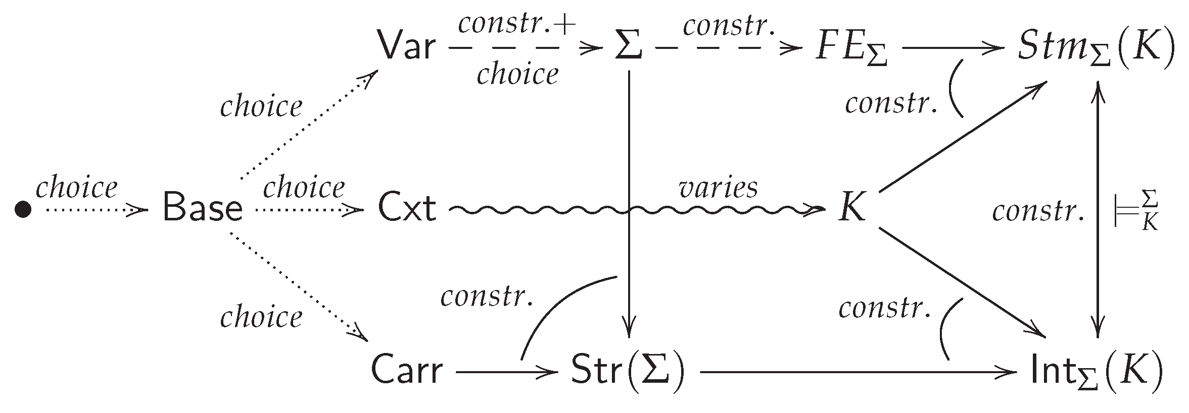
Disclaimer/Publisher’s Note: The statements, opinions and data contained in all publications are solely those of the individual author(s) and contributor(s) and not of MDPI and/or the editor(s). MDPI and/or the editor(s) disclaim responsibility for any injury to people or property resulting from any ideas, methods, instructions or products referred to in the content. |
© 2026 by the authors. Licensee MDPI, Basel, Switzerland. This article is an open access article distributed under the terms and conditions of the Creative Commons Attribution (CC BY) license (http://creativecommons.org/licenses/by/4.0/).
Copyright: This open access article is published under a Creative Commons CC BY 4.0 license, which permit the free download, distribution, and reuse, provided that the author and preprint are cited in any reuse.


