

Submitted:
03 July 2026
Posted:
03 July 2026
You are already at the latest version
Abstract
This study presents a mathematical modeling framework to analyze the impact of integrating sterilizing treatment into tuberculosis (TB) control strategies, particularly in resource-limited settings. Our findings highlight that while sterilizing treatment alone is highly effective in reducing TB incidence and mortality, its widespread implementation requires significant financial investment. The optimal control approach demonstrates that a mixed strategy, combining sterilizing and non-sterilizing treatments, can achieve comparable public health benefits at a lower cost, especially in the medium-term planning. From a long-term perspective, however, our results suggest that exclusively sterilizing treatment ultimately leads to greater reductions in TB incidence, prevalence, and mortality, justifying its higher initial cost. This is primarily due to the ability of sterilizing drugs to eliminate latent TB infections, prevent future active infections and disease-induced deaths, and avoid a considerable number of treatments. Additionally, under scenarios where the cost of sterilizing drugs decreases over time, a swift transition to a solely sterilizing treatment could result in both epidemiological and economic advantages for healthcare systems.
Keywords:
tuberculosis transmission model
; non-sterilizing and sterilizing treatment
; optimal control
; budget constraint
; epidemiological assessments
1. Introduction
Tuberculosis has been a significant public health concern for centuries, and it remains a burden in many middle- and low-income countries. Tuberculosis (TB) is a bacterial infectious disease caused by Mycobacterium tuberculosis (Mtb), a rod-shaped (bacillus) bacterium also known as Koch’s bacilli. It primarily affects the lungs (pulmonary TB) but can also spread to other organs (extrapulmonary TB). TB is transmitted through airborne droplets when an infected person coughs, sneezes, or speaks, releasing tubercle bacilli into the air.
Notably, TB infections can be latent or active. Latent TB infection leaves the bacilli dormant in the body without causing symptoms, but they can reactivate, mainly due to malnutrition, comorbidities, or immunosuppressive treatment. Latently infected individuals are not infectious; they do not transmit the bacilli to others. People with active bacilli that multiply in their bodies are said to undergo active TB infection. They are contagious and usually show symptoms, such as persistent cough, weight loss, fever, and night sweats. A simple X-ray test may confirm the presence of active bacilli at an earlier non-symptomatic disease stage. However, health insurance will only cover such an X-ray test if a person exhibits some alarming symptoms. Thus, only symptomatic patient may receive treatment in many middle- and low-income countries. If untreated, TB can be fatal.
Understanding the distinction between sterilizing and non-sterilizing activities of antituberculous drugs is crucial in treating active TB infections. Sterilizing activity refers to a drug’s ability to eliminate all persistent bacilli (both active and dormant) that can cause relapse if not eradicated. On the other hand, non-sterilizing (or bactericidal) activity targets actively replicating bacteria, reducing the bacterial load but not necessarily eliminating all dormant forms [1,2,3]. It is also important to underline that there is no long-lasting immunity to TB after recovering from an active disease.
In simpler terms, sterilizing treatment leaves the patients bacilli-free by eradicating all active and dormant bacilli. In contrast, after the completion of non-sterilizing treatment and the disappearance of all the disease symptoms, some dormant bacilli may remain in the patient’s body and become active when the patient’s immune system is weakened. In other words, patients who received non-sterilizing treatment turn latently infected after completing the treatment.
The standard strict-scheme course of sterilizing TB treatment approved by the World Health Organization [4], is based on a combination of rifampicin (replaceable by rifapentine or rifabutin) and pyrazinamide, both featuring a strong sterilizing effect, and twp bactericidal drugs (usually isoniazid and ethambutol). Among these drugs, rifampicin and its analogs are the most expensive, and healthcare entities in middle- and low-income countries may not have sufficient funds for their acquisition. As a result, many patients in such countries receive non-sterilizing TB treatment with cheaper bactericidal drugs only. In many middle- and low-income countries, there are no programs aimed at detection of latent TB infections, and such infections may only be occasionally discovered, e.g., before an immunosuppressive treatment for some comorbidities is to be assigned. In general, latent TB is not considered “sickness” because of no symptoms it brings forward for justifying the medical test to run. Thus, we actually have no estimation of how many latent TB infections there are, and the outcomes of non-sterilizing treatment may also leads to the accumulation of latently infected people who may become actively infected later in life, especially when their immune status changes.
Several studies (see [5,6] and references therein) highlight that COVID-19 provoked active TB infections in latently infected individuals through immune suppression, lung damage, immunosuppressive treatments, and socioeconomic stressors during the pandemic attributed to the limited access to healthcare facilities, lack of medical personnel and laboratory space, as well as poverty increase due to economic problems caused by quarantine. This effect was more visible in high-TB burden regions composed of middle- and low-income countries, where latent TB is common. As a result, TB morbidity notably increased in such regions [4]. Therefore, reduction of the latent TB infections is crucial for global TB control and eventual eradication, and healthcare entities should try to provide sterilizing treatment to actively TB-infected patients whenever possible.
This paper addresses the challenges related to the introduction of sterilizing treatment from a mathematical standpoint while also considering the limited funds available for TB treatment in middle- and low-income countries. Our goal is to showcase the future benefits of not only switching entirely to sterilizing therapy (which is an ideal case) but also to assess the effect of implementing a variable (non-constant in time) distribution between the two treatment types within the limits of an assigned budget. Such a distribution has been designed using the optimal control approach.
The paper is organized as follows. Section 2 presents the new TB transmission model featuring two classes of treated individuals, where a constant share defines the distribution between the two treatment types. In Section 3, we conduct the local analysis of the introduced model, including the computation of its basic reproductive number and possible equilibria, and analyze the long-term behavior of the model with a constant share of new patients to undergo each type of treatment.
In Section 4, we introduce a time-variable share that defines the distribution between the two treatment types and formulate an optimal control problem of finding an optimal share that minimizes the total number of new latent and active TB infections under a budget constraint. We also justify the existence of the optimal solution to the underlying optimal control problem and anticipate its structure.
The main practical results are gathered in Section 5. In SubSection 5.1, we estimate and compare the outcomes of both treatment types (solely non-sterilizing and solely sterilizing) from the short-, medium-, and long-term perspectives. Such estimations are then contrasted with those obtained for the optimal time-dependent distributions between the two types of treatment, which are designed based on the optimal control approach. The latter is performed in SubSection 5.2, where we showcase and discuss the numerical solutions to the optimal control problem under budget constraints while assuming the relative costs of sterilizing drugs are either constant or decreasing in time. A practical outlook of the numerical results is given in SubSection 5.3.
Finally, the key outcomes of the present work are outlined in Section 6.
2. The TB Transmission Model with Two Treatment Types
Taking as the basis a simple model developed in [7] that only features non-sterilizing treatment, we now propose its extension that helps model the introduction of sterilizing treatment while still accounting for patients undergoing the habitual non-sterilizing treatment. Our model includes five time-dependent variables or classes of human individuals, each describing a particular group of people detailed below:
- – the number of susceptible people (free of bacilli).
- – the number of latently infected people (non-infectious carriers of inactive bacilli) with no disease symptoms.
- – the number of infected people (infectious carriers of active bacilli) who have disease symptoms but are not being treated yet.
- – the number of individuals receiving non-sterilizing treatment.
- – the number of individuals receiving sterilizing treatment.
It is worth pointing out that during the initial phase of treatment (either sterilizing or not), patients may still be infectious, but as the treatment progresses, their infectiousness decreases. Therefore, we may assume that people from the classes and exhibit reduced infectivity, i.e., they are partially infectious.
We also suppose that all five classes are well-mixed and that the disease is transmitted only through encounters between infectious and non-infectious individuals. The total human population is denoted by
for all . The dynamic interflow between five disjoint classes and is expressed through by the dynamical system
with nonnegative initial conditions
The last initial condition in (3) implies that no patients are undergoing sterilizing treatment at the moment , and this type of treatment is just being introduced at .
Figure 1 displays the flow diagram of the TB transmission model (2), and the detailed descriptions of the model’s parameters are given in Table 1.
Let us briefly explain the model (2), paying attention to its novelty compared to the one developed in [7]. First, in the model (2), we have a share of infectious people who are assigned to undergo the sterilizing treatment (per unit time), while the rest of contagious individuals, , will be sent for habitual non-sterilizing treatment (see Eqs. (2d) and (2e) above). Thus, when , we have for all , and the system (2) is reduced to the one thoroughly studied in [7].
Second, we also assume that the rates of treatment completion and abandonment are different for the patients from class undergoing non-sterilizing treatment () and those from class assigned for sterilizing treatment (). It should also be noted that, after completing the treatment, people from the class become non-infectious but still latently infected (see Eqs. (2d) and (2b)) while people from the class become bacillus-free (see Eqs. (2e) and (2a)). However, by abandoning either treatment type, the patients become actively infected (see Eqs. (2c)-(2e)).
Third, as indicated in [8], patients may remain contagious for some time under both types of treatment, but their infectiousness gradually decreases as the treatment progresses. Let us also recall that non-sterilizing treatment makes the bacilli dormant or inactive while sterilizing treatment kills them. Therefore, it is fair to assume that the infectiousness of people undergoing treatment and belonging to the classes and is reduced, respectively, by factors and satisfying the relationship
which stays in line with experimental observations [3,9] and is reflected by Eqs. (2a)-(2c), where the mass-action incidence models the disease transmission through the term with denoting, as in [7], the “per capita rate of effective respiratory contacts with infectious people”. Thus, using this definition of introduced in [7] we have
Since there is no evidence of vertical TB transmission [10], we assume that all newborns, recruited at the constant rate , are bacillus-free. Here, we assume all individuals have the same natural mortality rate denoted by , while individuals from class I additionally exhibit the disease-induced mortality rate denoted by .
After inhaling active bacilli, a susceptible person from the class S, may either enter the I-class of contagious people with a probability by acquiring an active TB form or pass to the L-class with a probability by getting a latent TB infection. Here, the probability p of becoming actively infected and infectious depends on the immune response of the person receiving active bacilli. If a person’s immune system is weakened by comorbidities, malnutrition, or immunosuppressive treatments (for HIV, cancer, or transplants), this person has a higher risk of developing an active TB form [11,12].
People belonging to the class L of latently infected may develop an active TB infection if their immune status gets altered. In such a case, they will progress to the infectious class I at a rate (see Eqs. (2b)-(2c)). In other words, latently TB infected individuals may remain non-infectious during the time before developing an active TB infection.
Contagious people (class I) are then assigned for either sterilizing or non-sterilizing treatment at a rate . Thus, a share q of them passes to the class , and a share passes to the class (see Eqs. (2c)-(2e)). It is worth noting that people carrying active TB bacilli may remain untreated for a time during which medical test are run to confirm the disease and the treatment is assigned.
The well-posedness of the model (2) is guaranteed by the following statement.
Proposition 1.
Solution to the dynamical system (2), corresponding to any set of nonnegative initial conditions (3), is unique, nonnegative, and bounded for all .
The proof of Proposition 1 is almost identical to the one presented in [7] and therefore is left to the readers. Furthermore, Proposition 1 also entails the existence of a biologically meaningful region
which is positively invariant and constitutes the absorbing set of the system (2) because it contains all possible solutions of (2) engendered by the initial conditions satisfying the inequality . Therefore, must contain all possible equilibria of the system (2).
3. Local Analysis of the Model
The steady states or equilibria of the dynamical system (2) are its constant solutions and can be obtained by solving the following algebraic system:
In this section, we will identify the steady states of the dynamical system (2) as nonnegative solutions of the nonlinear system (Section 3) belonging to the absorbing set , which was defined by (4) in the previous section.
3.1. Disease-free equilibrium and basic reproductive number
For the system (2), the disease-free equilibrium (DFE), denoted by , can be obtained by setting the coordinates of all infective classes to zero, that is, by substituting in (Section 3). As a result, we have
which is nonnegative and belongs to the absorbing set .
One of the fundamental concepts in the epidemiology of infectious diseases is the basic reproductive number, , which quantifies the transmission potential of an infectious disease within a susceptible population. This metric represents the average number of secondary infections generated by a single infected individual in a completely susceptible population [13]. From a mathematical standpoint, the basic reproductive number is usually calculated as the spectral radius of the next-generation matrix at the DFE [14]. According to this approach, we should first define a sub-vector containing the human compartments that carry the infection
Next, we extract four differential equations from the dynamical system (2) that correspond to the components of and write them in the form
where
It is worth noting that stands for the rate of appearance of new infections (i.e., the disease transmission) and accounts for the disease transition rate. Both indicated inequalities are understood in the “component-by-component” sense.
According to [14], the next-generation matrix is defined by where and are the Jacobian matrices of and evaluated at the disease-free equilibrium , that is,
To simplify our calculations, we introduce the following notations for the four positive elements located on the main diagonal of
so the determinant of becomes
The above form of will be used in Section 3.3 to simplify some computations in the sequel. However, one can also obtain an equivalent form of (7) that reveals that , and, therefore, is helpful for further analysis. Indeed,
Thus, let us introduce the following notation
where admits either the form (7) or
as derived above. To write the next-generation matrix in a more compact form, let us introduce the following auxiliary quantities:
Then, we can write the next-generation matrix as
The characteristic polynomial corresponding to is
and using the left-hand relationship in (10), we have
According to the structure of , three eigenvalues of are zero, and the positive one is precisely equal to the spectral radius of , that is
Thus, we arrive at the basic reproductive number, for the TB transmission model (2) that expresses a mean number of secondary TB infections produced by one infectious individual when introduced into a totally susceptible population:
3.2. Existence of the Endemic Equilibrium
To obtain another feasible solution of the nonlinear system (Section 3), we start from the equations (5a), (5d), and (5e) and express
Then, by substituting (13a) and (13b) into (5b) we can also express
Now, we substitute the quantities , , and given by (13a), (13b), and (13d) into equation (5c) and get
An obvious solution of the above equation leads us to the disease-free equilibrium , while its other possible solution(s) must satisfy the equality
Note that the above equation is linear with respect to . Using the definitions of and E given in (12) and (8), respectively, we can express its independent term as
and its leading coefficient as
Thus, (14) can be written in the following form:
meaning that a unique solution of the linear equation (14) is
Notably, when , we have that . Comparing the expression for given by (15) with the one in formula (13c), we can write
Rearranging some terms in the last expression and substituting and from (13a) and (13b), we then obtain
Again, using the definitions of and E given in (12) and (8), we arrive at
from where the coordinate is finally expressed as
To establish the sign of the denominator in (16), we recall that and . Hence,
because the parameters are nonnegative. Furthermore, using the definition of E given by (8) we have
Thus, it holds that
meaning that defined by formula (16) is positive only if
From the preceding rationale and to culminate this section, we formulate the following statement concerned with the existence of equilibria of the TB transmission system given by (2).
Proposition 2.
If , the system (2) has only the disease-free equilibrium . If , the system (2) has two equilibria: the disease-free equilibrium and the endemic (strictly positive) equilibrium whose coordinates are defined by
A formal proof of Proposition 2 is provided in Appendix A.
3.3. Long-Term Behavior of the TB Transmission Dynamics
According to Proposition 2, the TB transmission system may possess either one or two equilibria, whose existence is determined by the threshold value of basic reproductive number defined by (12), which also plays a crucial role in the long-term behavior of the solutions of the system (2).
It is worth recalling that if , then each contagious individual induces less than one new infection, on average, during their infectious period, meaning that the disease will disappear sooner or later regardless of its current state. From the mathematical perspective, it can be expected that the trajectories of the system (2) would eventually converge to when as is the only equilibrium that exists when .
On the other hand, if , then each contagious individual induces more than one new infection, on average, during their infectious period, meaning that the disease will persist because new infections will consequently arise. In other words, the trajectories of (2) will converge to the endemic equilibrium with strictly positive coordinates defined by (2), thus diverging from the DFE, .
To formalize this intuitive rationale, we formulate the following result.
Theorem 1.
The long-term evolution of the system (2) depends on the threshold value of the basic reproductive number defined by (12) in the following sense:
- (i)
- When , the disease-free equilibrium is globally asymptotically stable (or GAS) on the absorbing set given by (4).
- (ii)
-
When , the disease-free equilibrium is unstable, and the endemic equilibrium with strictly positive coordinates defined by (2) is GAS on the open subset defined bybelonging to the absorbing set Ω.
A formal proof of Theorem 1 is provided in Appendix A.
From the common-sense standpoint, allowing for any equilibrium in which the disease will always persist is undesirable. Therefore, instead of paying too much attention to the stability properties of , we would like to focus more on achieving the disease-free state by adequately changing the parameter that mimics the assignment of actively infected people for sterilizing treatment.
In the next section, we propose employing the optimal control framework to obtain an optimal dynamic assignment for sterilizing treatment. We seek to minimize active and latent human TB infections while keeping the total costs of both treatment types (non-sterilizing and sterilizing) within a determined budget.
4. Optimal Control Approach
The share of infectious patients assigned for sterilizing treatment was assumed constant in the previous sections. However, this share can also be modeled by a piecewise continuous real function dependent on time . Thus, we introduce a control function that mimics the dynamic (time-variable) share of infectious patients who will further undergo the sterilizing treatment. In contrast, will model the time-variable share of infectious patients who will further undergo non-sterilizing treatment. As both and are piecewise continuous and bounded to the range , replacement of q by in the dynamical system (2) will not alter the existence and uniqueness of its solution, and will remain being the absorbing set of the controlled system
for all admissible piecewise continuous real functions defined for
The choice of the control function can pursue one or more desirable (but also realistic) goals that will benefit public health. In particular, the costs of sterilizing and non-sterilizing treatment may be essential in choosing . In this context, it is worth noting that sterilizing TB treatment is usually more expensive than non-sterilizing treatment, even though the total duration of both treatment types is basically the same [15,16].
To model the introduction of sterilizing TB treatment, we assume that the observation period starts at and ends at where T is fixed. We also suppose that before the observation period , all actively infected people have been receiving only non-sterilizing treatment. This leads us to assign the following initial conditions to the controlled system (Section 4)
such that
Here, it is essential to point out that all people undergoing treatment at should continue receiving non-sterilizing drugs, meaning that they may either become latently infected (L-class) after completing the treatment or become actively infected (I-class) in the case of treatment abandonment.
In this section, we propose modeling the introduction of sterilizing TB treatment, while assuming that the additional costs related to the use of sterilizing drugs must be covered by the budget allocated for the habitual use of non-sterilizing drugs (budget constraints). This approach appears more realistic and practical in application, even though it requires solving an optimal control problem with a budget constraint.
Let denote a piecewise continuous control function and be a fixed observation interval. The purpose of control consists in minimizing the number of actively and latently infected people during the observation period, expressed by the objective functional:
where defines the priority of minimizing the current number of actively infected individuals over the latently infected ones because the former ones do transmit the disease while the latter ones do not.
To introduce the budget constraints, we have to model the costs related to each treatment type. Here, we propose using relative costs and thus avoid dealing with absolute values of non-sterilizing and sterilizing drugs that differ from country to country.
First, we note that the treatment cost depends on the dynamic compartments , which contain all people undergoing treatment. Suppose we have the time interval as a planning horizon and, for simplicity, assume that the cost (per individual) related to the non-sterilizing treatment of one patient entering the class is normalized to unity. If only non-sterilizing treatment is assigned to all identified infectious individuals (meaning that and for all ), then instantaneous cost is equal to , and the cumulative cost related solely to non-sterilizing treatment can be assessed by the integral
which will serve as the “baseline cumulative cost”. Notably, in (22) is the solution to the system (Section 4) with .
As sterilizing drugs are more expensive compared to non-sterilizing ones [15], we may also assume that the cost (per unit time) related to the sterilizing treatment is -times more expensive with compared to non-sterilizing treatment. For example, implies that sterilizing drugs are twice as expensive as non-sterilizing drugs.
On the other hand, a recent WHO report [4] highlights the ongoing efforts to reduce the cost of sterilizing TB drugs, emphasizing partnerships like the Global Drug Facility to negotiate lower prices and improve affordability in low- and middle-income countries. Currently, the key sterilizing TB drugs (such as pyrazinamide and rifampicin) remain rather expensive, primarily due to the patent protections and limited generic production. However, advocacy campaigns are pressuring manufacturers to reduce prices and increase the accessibility of sterilizing TB drugs by increasing their generic production [17]. All these actions raise hope that the prices of sterilizing TB drugs may gradually go down in the future. To model such a situation, we can define the relative cost (per unit time) of sterilizing treatment using a decreasing function depending on time (see Figure 2), that is,
This function can be used to define two scenarios related to the relative cost of sterilizing treatment, namely:
- Constant cost.
- In this case, we assume and , meaning that the relative (per unit time) cost of sterilizing treatment remains constant during the entire observation period .
- Decreasing cost.
- In this case, we assume and in (23), meaning that the relative (per unit time) cost of sterilizing treatment is a monotone decreasing function of time .
At the beginning of this section, we introduced a piecewise continuous control function that mimics the dynamic (time-variable) share of infectious patients who will further undergo the sterilizing treatment, while models the time-variable share of infectious patients who will further undergo non-sterilizing treatment. Therefore, the instantaneous cost related to both types of treatment is
To assess the cumulative total cost related to both treatments for a given , we employ the following integral
where is the solution to the system (Section 4)-(Section 4) for a given , while is defined by (23). Here, we also recall that the cost (per individual) related to the non-sterilizing treatment is normalized to unity.
Using the baseline cumulative cost B defined by (22), we can now formulate the budget constraint expressing that the additional expenses related to the use of sterilizing drugs must come from the budget calculated for the habitual use of non-sterilizing drugs
where the constant can be either zero or positive and thus be adjusted to either constant or decreasing costs described above. The integral constraint defined by (25) (known as an isoperimetric constraint in the optimal control theory) must be satisfied alongside the dynamics of the controlled system (Section 4)-(Section 4). Notably, the constraint (25), when added to the optimal control problem, will narrow down the class of admissible piecewise continuous control functions and their corresponding states , which are solutions to the dynamical system (Section 4)-(Section 4). However, this constraint is feasible in the sense that there exists at least one control function (namely, for all ) that fulfills it (cf. relationship (22)).
Taking into account the constraint (25), the underlying optimal control problem can be formulated as follows. For each , find an optimal share of individuals from the class to undergo a sterilizing TB treatment to minimize the objective functional (21) subject to the dynamical system (Section 4)-(Section 4) together with the constraint (25).
Dealing with the budget constraint (25) is challenging. However, as stipulated in [18], an inequality-type constraint can be “merged” into the objective using a Lagrange multiplier thus forming the “augmented objective” (or Lagrangian functional), that is,
where the constant term is of no concern for minimization. The multiplier is chosen to satisfy the complementary slackness condition
at the optimal control . If the budget is inactive at the optimum (meaning the inequality (25) is strict in ), then and the problem reduces to the unconstrained minimization. However, if the budget is active, then is chosen so that the budget inequality (25) holds as equality at .
Remark 1.
Remark 2.
To account for the budget constraint (25), we formulate the optimal control problem in a slightly different form. For each , find an optimal share of the actively infected and symptomatic individuals from the class to undergo a sterilizing TB treatment to minimize the augmented objective functional (26) with satisfying the complementary slackness condition (27), on the solutions to the ODE system (Section 4) with initial conditions (Section 4).
This problem can be formally solved by applying the Pontryagin minimum principle (see, e.g., [18,19] or other similar textbooks). However, one has to recall [18] that the necessary condition for the solvability of the optimal control problem (Section 4)-(21) is the solvability of the initial value problem (Section 4)-(Section 4) for any piecewise continuous control function together with the boundedness of all its possible trajectories . To validate this necessary condition, we formulate the following result.
Proposition 3.
Proof.
The initial value problem (Section 4)-(Section 4) can be written as
where is the vector function of the right-hand sides of the controlled dynamical system (Section 4). This vector field is locally Lipschitz in and for any measurable defined for , and the Carathéodory existence and uniqueness theorem applies [20,21]. Therefore, a unique solution exists for any initial condition and for all measurable . Furthermore, in light of Proposition 1 and the property (20b), all the solutions of the form are bounded and belong to the closed set defined by (4). □
After establishing the solvability of the controlled dynamical system (Section 4)-(Section 4) for all measurable defined for , including piecewise continuous functions, we formulate the following statement to ensure the existence of an optimal control that minimizes the augmented objective functional (26) subject to the dynamical system (Section 4)-(Section 4).
Proposition 4.
Proof.
The existence of an optimal control belonging to the class of measurable (that is, integrable) functions, can be proven by applying the standard result [22,23], according to which the fulfillment of certain conditions will be sufficient for the existence of an optimal control. In our case, the validity of the following conditions will suffice to guarantee the existence of an optimal control:
- (i)
- (ii)
- Compactness and convexity of the control set. Since , the control set is bounded and convex.
- (iii)
- (iv)
- (v)
- Lower semicontinuity of the objective functional. The value of is bounded by from below.
Finally, the absorbing set defined by (4) is convex for any and for all , and the existence result from [22] (see Theorem 9.3.i) is applicable. The latter, together with the validity of conditions (i)-(v) ensures the existence of that minimizes the augmented functional (26) over any finite time interval subject to the dynamical system (Section 4) with initial conditions (Section 4).
It is also important to point out that the formulated optimal control problem with budget constraint is feasible in the sense that there is at least one control function () that satisfies the budget constraint (25). □
Once the existence of optimal control is proved by Proposition 4, we proceed to formulate the necessary condition of optimality in the form of the Pontryagin minimum principle (see, e.g., [18,19] or similar textbooks). Here, the Hamiltonian corresponding to the optimal control problem (Section 4)-(21) is
where stands for scalar product, is the vector field of the system (Section 4), and denotes the vector of co-states (or adjoint variables) corresponding to the state variables . In the above expression, the co-state vector function is absolutely continuous and satisfies the adjoint system with transversality condition
Note that the detailed form of (29) is provided in Appendix B.
The optimal control whose existence was proved by Proposition 4 must satisfy the Pontryagin minimum principle, which is a necessary condition of optimality. Therefore, almost at each along the optimal path , the Hamiltonian (28) must fulfill the condition
Here, it is worth noting that Hamiltonian is linear in u, and its partial derivative
is independent of u, meaning that attains its minimum with respect to u at the extreme points of the closed interval . From this rationale, it stems that
where
denotes the switching function that represents the right-hand side of the relationship (30) evaluated at each From the expression (32), we can see that the sign of the switching function is defined by the relationship between the extra cost, weighted by , and the adjoint functions and corresponding to both types of treatment.
Let us recall the meaning of the adjoint functions and associated with the state variables and . In general terms, adjoint variables encode how changes in the final state () propagate backward in time to influence the optimal control trajectory and the value of the objective functional. As the adjoint variables are determined by backward integration (see Eq. (29) above), their values reflect how the future goals (e.g., minimizing the cumulative number of all active and latent TB infections and the compliance with the budget, both expressed via in (26)) influence the present-day decisions. Here, the decision is to distribute all infectious TB patients to undergo either sterilizing or non-sterilizing treatment. Thus, and quantify how increasing the number of individuals assigned for non-sterilizing and sterilizing treatment ( and , respectively, at each ) will affect the cumulative number of infections while complying with the assigned budget.
Furthermore, each adjoint variable can be interpreted as a shadow price representing the opportunity value of increasing the corresponding state variable at a given time t by one unit (ceteris paribus). From this angle, the quantities and express the opportunity values of adding one individual to the class and on the overall objective. Revising the formulas (31) and (32), one may easily guess that, for each single , the relationship will lead to employing the non-sterilizing treatment, while will motivate for the sterilizing treatment. Here, the multiplier also acts like a shadow price per unit of extra sterilizing-treatment cost, because it may shift the switching threshold.
Thus, the optimal control expressed by (31) is piecewise constant and switches between two regimes: (only sterilizing treatment) and (only non-sterilizing treatment). The number of switchings is defined by the number of roots of the switching function (32) and depends on the relative magnitude of and at each . This type of optimal control is referred to as “bang-bang” with the switchings occurring at the isolated points when , or equivalently when . The latter implies that both treatment types render the same opportunity value at while these values change at for arbitrary small .
Remark 3.
From the theoretical standpoint, there may exist an interval with where it holds for all (meaning that vanish within ). In such a case, the optimal control may admit interior values when , that is, , meaning that it is optimal to assign both types of TB treatment during the period . Situations like this are less probable than the straightforward bang-bang control, especially in our case, because of the form of the switching function (32) that explicitly includes the non-increasing cost function and the constant multiplier η. Still, they may eventually take place and are known in the literature as singular arcs (see more details in [24] and similar textbooks).
Given the nonlinearity of the optimal control problem (Section 4)-(26) and the complexity of the adjoint system (29) (see its detailed form in Appendix B), the optimal control and corresponding optimal states can only be found numerically. Nonetheless, the general structure of formalized by (31) and predicted by the Pontryagin minimum principle will serve as a reference to validate its numerical solution, which will be provided in the next section.
5. Numerical Solutions and Discussion
Let us recall that, according to [4], a combination of four drugs (rifampicin, pyrazinamide, isoniazid, and ethambutol) is necessary for the standard strict-scheme course of sterilizing treatment. If one or more drugs become (temporarily or permanently) unavailable to a patient, the treatment may lose its sterilizing effect and become non-sterilizing. This is precisely what is observed in many low- and middle-income countries due to the deficit of rifampicin, the most powerful first-line anti-TB sterilizing drug. Its intermittent presence or absence in the proper treatment scheme usually leads to non-sterilizing treatment based on three other drugs (isoniazid, pyrazinamide, and ethambutol) that are more accessible and cheap.
From this rationale, we can safely assume that both treatment types (sterilizing and non-sterilizing) have about the same duration, usually about 6 months [4], and the treatment escape rate can also be assumed the same for both treatments as the patients usually are not aware of the treatment type they receive. These two assumptions will remain valid for all numerical simulations presented in this section, along with the values of the parameters of the dynamical systems (2) and (Section 4), which are displayed in Table 2.
In [8], it was shown that both treatment types reduce the infectiousness of patients with active TB forms with solely sterilizing treatment contributing a bit more to such reduction [3], we focus on the “pessimistic” scenario and assume in numerical simulations. We also suppose that treatment is assigned immediately after clinical tests confirm the presence of active bacilli, so the time between the beginning of the infectiousness and the commencement of therapy, , is around two months.
Numerous studies have revealed that tuberculosis tends to have a notably higher incidence in bigger cities (1 million inhabitants or more), featuring social disparities. Using the values of and given in Table 2, we can model the total human population of about million inhabitants. Thus, we take
and close to million inhabitants. At the same time, the TB transmission rate, , is chosen to fit the annual TB incidence rate of around 200 cases per inhabitants. We have also assumed that initial conditions (Section 4) assigned to the ODE system (Section 4) are close to the endemic equilibrium (2) of the system (2) with , namely:
In the sequel, we provide numerical simulations when the share of actively TB-infected patients to undergo the sterilizing treatment is either constant, or variable in time, .
5.1. Useful Insights from ODE System (2) with Constant
To show off the expected effect of sterilizing TB treatment, we present the evolution of the basic reproductive number as a function of the parameter (the share of actively infected TB patients assigned for the sterilizing treatment), that is, using the formula (12). Here, we employed the values of parameters of the model (2) defined in Table 2. The function is displayed in Figure 3, where meaning that if only the non-sterilizing treatment () is given to all actively-infected TB patients, the disease will persist. However, if or more () of such patients will undergo the sterilizing treatment, there is a perspective to eradicate the disease ().
Notably, is a decreasing function of (see Figure 3). Therefore, the greater the share of actively TB-infected patients assigned for the sterilizing treatment, the sooner the disease eradication can be achieved. The latter highlights the benefits of sterilizing TB treatment.
To quantify the effect of variations in model parameters on disease transmission potential, we conducted a sensitivity analysis of using the parameter ranges listed in Table 2. The method described in [33,34] was applied to estimate the first-order and total-order sensitivity indices of the basic reproduction number. The analysis was based on simulations, accounting for the variability of all model parameters. The first-order indices represent the direct contribution of each parameter to the variance of , excluding interaction effects with other parameters. The results presented on the left-hand chart of Figure 4 reveal that only a few parameters exert a substantial direct influence on , as summarized below:
- (recruitment rate of individuals): (95% CI: –) exerts the strongest direct influence on .
- (transmission rate): (95% CI: –) plays a significant role in determining the transmission dynamics.
- q (fraction of patients receiving sterilizing treatment): (95% CI: –) has a notable effect, although with considerable uncertainty.
- (rate of screening/recruitment for treatment): (95% CI: –) shows a moderate but non-negligible impact.
- (rate of slow infection progression): (95% CI: –) contributes weakly, with higher uncertainty.
- Other parameters (, , , p, , , , , , ) exhibit negligible direct contributions.
The total-order indices reflect the contribution of each parameter, including its interactions with all other parameters. Unlike the first-order indices, which measure the effect of varying one parameter at a time while keeping the others fixed, the total-order indices capture the combined influence that emerges when all parameters vary simultaneously. This provides a more realistic assessment of parameter importance under joint uncertainty. As shown in Figure 4 (right chart), the parameters with the highest total-order sensitivity indices are detailed below:
- q (fraction of patients receiving sterilizing treatment): 0.40 (95% CI: 0.32 – 0.48) indicates that, beyond its direct effect, it also interacts significantly with other parameters.
- : 0.37 (95% CI: 0.25 – 0.46) keeps its robust effect.
- : 0.26 (95% CI: 0.16 – 0.36) maintains its key role in the sensitivity of .
- : 0.12 (95% CI: 0.05 – 0.20) gains importance when interactions are considered.
- The remaining parameters (, , , , , , , , ,, p) show values close to zero in their total indices, indicating a marginal influence.
To summarize, the basic reproduction number exhibits the highest sensitivity to the fraction q of infectious individuals assigned to sterilizing treatment when all the model’s parameters vary within their respective ranges. Namely, by increasing q, the value of will decrease even if other parameters of the model are perturbed, and the situation shown in Figure 3 is expected. It implies that, from an epidemiological perspective, interventions aimed at increasing the sterilizing treatment coverage will have a significant impact on reducing and mitigating the disease propagation.
It is also relevant to consider two borderline scenarios, namely:
- 1.
- All actively TB-infected patients will undergo the non-sterilizing treatment ( in system (2)).
- 2.
- All actively TB-infected patients will undergo the sterilizing treatment ( in system (2)).
These two borderline scenarios may give us the worst- and best-expected outcomes regarding disease propagation and persistence in the short-, medium-, and long-term perspectives.
Numerical simulations of the dynamical system (2) with constant (solely non-sterilizing treatment) and (solely sterilizing treatment) are presented in Figure 5, using blue and red curves, respectively. The left- and right-hand charts in Figure 5 correspond to the solutions and of the ODE system (2), respectively. Besides fully agreeing with the expected value of (cf. Figure 3), the graphs in Figure 5 clearly reflect the benefits of sterilizing treatment () compared to a non-sterilizing one (). In effect, the use of solely non-sterilizing treatment leads to the endemic persistence of the disease (see the blue-colored curves in Figure 5), while solely sterilizing treatment is capable of reducing rapidly the current number of latent and active TB infections even in a short-term perspective (cf. the difference between the blue- and red-colored curves in Figure 5 at years, marked by the dashed vertical lines). Moreover, the benefits of solely sterilizing treatment () become more visible in the medium- and long-term perspective if we compare the blue- and red-colored curves in Figure 5 at and .
It is worthwhile to highlight that the numerical outcomes displayed in Figure 5 fully agree with the theoretical results presented in Section 3 and Section 3.3. When , we have (see Figure 3) and the trajectories of the ODE system (2) converge to the endemic equilibrium defined by (2). In contrast, when , we have (see Figure 3) meaning that does not exist (as affirmed in Proposition 2) and the trajectories of the ODE system (2) should converge to , its unique equilibrium, when This conclusion is perfectly consistent with Theorem 1.
There are other important dynamic indicators that help visualize the potential outcomes of both TB treatment types. Among them, we choose for illustration the following:
- Cumulative number of latent TB infections, , arising during the period as a result of contagion or non-sterilizing treatment, is defined bywhere are solutions to the system (2) with either or
- Cumulative active TB incidence, , which sums up all new active TB infections that occur during the period , is defined bywhere are solutions to the system (2) with either or
- Cumulative TB-induced mortality, that sums up all TB-induced death cases that appear during the period is defined bywhere I the component of the solution to the dynamical system (2) with either or .
Figure 6 displays the graphs for and . Even though the reduction of cumulative active TB incidence, , and the disease-induced mortality, , is relatively moderate during the short-term perspective (as marked by the vertical line in all three charts), such a reduction becomes more visible in the medium- and long-term perspectives.
Moreover, the cumulative latent TB incidence, , exhibits a noticeable decrease when (see the left-hand chart in Figure 6). Numerical estimations of the key quantities and that can be contrasted by comparing the end-point at of the blue and red curves in the left and right columns of Figure 6, are provided in Table 3 (three upper rows). Furthermore, using a rule similar to (Section 5.1), we can also assess other important quantities characterizing the sole use of either non-sterilizing or sterilizing treatment for active TB infections. Namely, we can estimate:
- The total number of treatments started during the period is defined by
- The total number of treatment dropouts during the period is defined by
- The total number of treatment completions during the period is defined by
Numerical estimations of the three additional features defined above are also provided in Table 3 (three lower rows) for both treatment types and in the short, medium, and long-term perspectives. Thus, Figure 5, Figure 6, and Table 3 jointly showcase the benefits of the solely sterilizing treatment over the non-sterilizing one, when no extra cost for sterilizing drugs is involved. In other words, if the budget constraint (22) is ignored, meaning that the functional defined by (21) is minimized subject to the ODE system (Section 4), the optimal solution will always be for any length of the observation period ( or 30).
In the following subsection, we provide numerical solutions to the optimal control problem with a budget constraint and discuss how the additional cost of sterilizing drugs may affect the type of treatment assigned to new patients under short-, medium-, and long-term planning.
5.2. Numerical Solutions for Optimal Control
In Section 4, we proposed an optimal control approach for introducing sterilizing TB treatment under the budget constraint (22), which naturally depends on the planning horizon T. Similar to SubSection 5.1, let us focus on short-term ( years), medium-term ( years), and long-term ( years) perspectives and estimate the corresponding values of the budget using the formula (22), that is,
where is the solution to the ODE system (2) with (solely non-sterilizing treatment), while assuming that the cost (per unit time) related to the non-sterilizing treatment of one patient entering the class is normalized to unity. The baseline cumulative costs and defined above are obtained using the parameter values from Table 2 for and , respectively. They are then replaced in the constraint (25) and also in the augmented functional (26) together with the complementary slackness condition (27).
It is worthwhile to point out that we have set in the objective functional (26) for all numerical simulations to emphasize that minimizing active TB infections is 5 times more important than reducing latent TB infections because actively infected patients contribute a lot more to the infection spread compared to latently infected ones.
As a reference, we can also assess the cumulative costs corresponding to solely sterilizing treatment using the formula (24) with . In Section 4, we considered two cases (constant and decreasing costs, see p. Section 4) corresponding to the constant and decreasing relative costs of sterilizing treatment and expressed through the values of coefficients of the cost function defined by (23) (see also Figure 2). In the sequel, we determine the cost function for these two cases.
- Constant cost.
-
In this case, we assume in (23) and , meaning that the relative (per unit time) cost of sterilizing treatment remains is 20% or 50% more expensive compared to non-sterilizing treatment during the entire observation period , and for all the three perspectives: short-term ( years), medium-term ( years), and long-term ( years). Notably, such an increment of the relative cost of sterilizing treatment (20% to 50%) was estimated from a recent study by [16] that has taken into account the costs of two sterilizing drugs (Rifampicin and Pyrazinamide). These drugs are manufactured only in India, China, Europe, and the US, and their supply to other countries is somewhat intermittent. The prices of the four TB medications expressed in US dollars (data borrowed from [16]) are summarized in Table 4 below:Thus, we have two constant cost functions to test,
- Decreasing cost.
-
In this case, it is prudent to assume that the longer the observation period, the cheaper the relative cost of sterilizing treatment will be by the end of the observation period. Thus, for both values we can project that the relative costs of sterilizing and non-sterilizing become equal in years, that is . Under such an assumption, we then define two decreasing cost functions as follows:
Figure 8 displays the cost accumulations under solely non-sterilizing treatment (blue-colored curves) and solely sterilizing treatment with smaller constant and decreasing relative costs on the left (, red and yellow curves, respectively) and the larger ones on the right (, red and yellow curves, respectively). While in the short-term perspective ( years) the spending on sterilizing treatment always exceeds the baseline cost (blue curves in both charts), this tendency changes in the medium-term planning () if a smaller relative cost is assumed (meaning that either or is employed). However, if a larger relative cost is assumed (expressed by the cost functions or ), the spending on sterilizing treatment drops below the baseline cost only in the long-term perspective (). Moreover, in the long-term perspective ( years), the cumulative spending exhibits a notable reduction in all scenarios compared to the habitual practices of non-sterilizing treatment. Table 5 provides the details of cumulative spending given in Figure 8.
From Figure 8 and Table 5 we can easily guess that is the optimal solution in the long-term perspective ( years) and also in the medium-term perspective ( years) if either constant or decreasing relative cost of sterilizing drugs is assumed, that is, if the cost functions or are employed. In such scenarios, the budget constraint (25) becomes inactive, leading to in the complementary slackness condition (27).
Now, we focus on the numerical solving the optimal control problem with budget constraint (25) in the short-term perspective () with the relative costs defined by and and in the medium-term perspective () when the relative costs are higher, meaning that the cost functions and are employed.
All numerical solutions of the optimal control problem of minimizing the functional (26) subject to the dynamical system (Section 4) with initial conditions (Section 5) were obtained using following scheme, consisting of two steps.
In the first step, we apply direct time discretization to obtain a finite-dimensional problem. The solution to this problem provides an initial guess regarding the structure of the solution. Specifically, for our optimal control problem, we obtain a bang-bang control with two arcs. In the second step, we use the arc-parametrization method, as described in [35], to compute a refined optimal solution. Although sufficient conditions for the optimality of the bang-bang control are not formally proven here, such verification can be performed using the NUDOCCCS software developed in [36] and further employed in[37].
For the numerical implementation of both methods, we use the Applied Modeling Programming Language (AMPL), [38] in combination with the IPOPT solver [39]. The key parameters chosen are discretization points and an IPOPT tolerance of .
Table 6 summarizes the types of optimal solutions returned by the AMPL-NUDOCCCS solver. Even though all types of optimal control shown in Table 6 formally comply with the predicted form (31), there are only four scenarios where the optimal control exhibits the verily bang-bang form. Notably, for the two short-term scenarios ( years), the optimal bang-bang controls are almost identical, so the difference between them cannot be visually perceived. Therefore, we only show the graph of optimal control for the decreasing cost function in Figure 9 because for the constant cost function is almost identical. The only difference is the switching point , namely,
Figure 9 exhibits the bang-bang optimal controls (left column) and the corresponding switching functions (right column), obtained numerically using the formula (32).
Let us now discuss the results exhibited in all charts of Figure 9, starting from the upper row. Because the planning horizon is too short to reflect the long-term advantages of the costly sterilizing TB treatment, and the budget is constrained, this treatment is applied only during the first 18 or 22 days to stay within budget limits, while the shorter period corresponds to the constant lower cost and a bit longer period applies to the decreasing lower cost .
However, there is no way to match the budget constraint in the short-term perspective when the relative cost is assumed higher (that is, cost functions or are employed). In such situation, only non-sterilizing treatment has to be assigned to all patients with active TB to stay within the limits of the budget.
Nonetheless, from the outcomes of the short-term scenarios one can deduce that the smaller is the relative cost, the longer can be the period for applying the sterilizing treatment while satisfying the budget constraint. This tendency is also illustrated by the medium-term scenarios ( years), as shown in the middle and lower rows on Figure 9.
Indeed, when the relative cost of sterilizing treatment is higher and expressed by (see the charts (c) and (d) in Figure 9), this better kind of treatment can be assigned to all patients with active TB forms up to the middle of the observation period ( years ), while for a bit lower decreasing cost the application of sterilizing treatment may last far more without violating the budget as shown in the the charts (e) and (f) in Figure 9 where . Moreover, if a lower relative cost expressed by the function or is assumed, the budget constraint (25) becomes inactive leading to in the complementary slackness condition (27) and constant optimal control .
Notably, in the long-term perspective ( years) the optimal control becomes constant, regardless of the function expressing the relative cost of sterilizing treatment, meaning that all infectious patients can receive sterilizing treatment without surpassing the assigned budget. These outcomes plainly agree with two charts presented in Figure 8 that exhibit the cumulative relative costs by blue curves (baseline non-sterilizing treatment), yellow curves (lower-cost sterilizing treatment), and red curves (higher-cost sterilizing treatment) when for all . Since the yellow and red curves are below the blue ones on both charts of Figure 8 at years, the budget constraint is inactive in the case of the long-term planning. However, when years, the yellow curves are already below the blue ones while the red curves are still above them. Therefore, in the case of higher relative cost and medium-term planning (that is, with or and years), the bang-bang optimal controls help match the budget.
Furthermore, when years, the red curves in Figure 8 are well above the blue ones, while the yellow curves are slightly above the blue ones. Thus, in the case of lower relative cost and short-term planning (that is, with or and years), the bang-bang optimal controls also help match the budget.
Table 7 summarizes the core indicators of the four optimal controls exhibiting the bang-bang structure, while similar indicators for (solely non-sterilizing treatment with or and years) and for (solely non-sterilizing treatment with or and years) are presented in Table 3. Note that, in the long-term perspective ( years), these indicators are the same as presented in the fourth column of Table 5 as they do not depend on the cost function .
Keeping in mind a minimal difference between the optimal bang-bang controls corresponding to the lower relative cost functions and , we now compare the values of indicators presented in the second and third columns of Table 7 and observe that the decreasing nature of the cost function has a positive effect on these indicators even in a short-term perspective ( years). By contrasting the values of indicators in the second and third columns of Table 7 with their baseline quantities given in the fifth column of Table 3 corresponding to the solely non-sterilizing treatment, we can observe that the application of sterilizing treatment during only the first 18-22 day (in accordance with the optimal bang-bang controls presented in Figure 9(a)) may improve the epidemiological situation without incurring into extra-costs.
Under the medium-term planning ( years), the benefits of optimal bang-bang controls shown in the charts (c) and (e) of Figure 9 become more evident compared to the baseline case of solely non-sterilizing treatment, while total costs remain unchanged. Such benefits can be perceived by comparing the indicator values in the last two columns of Table 7 with their baseline quantities in the sixth column of Table 3. In other words, bang-bang optimal controls enhance the cost-effectiveness of treatment as they improve the indicators predicted in the baseline case at no extra cost.
Notably, under short-term planning ( years) and under medium-term perspective ( years) with a higher relative cost (bang-bang optimal control), the budget constraint (25) is active, meaning that the total budget is spent. However, if the relative cost of sterilizing treatment is moderate (that is, cost functions or are employed) or if the planning is done for the long-term perspective ( years), the optimal control is and with this control the budget constraint (25) becomes inactive, meaning that there will be surplus compared to the baseline budget. The latter emphasizes even more the cost-effectiveness of sterilizing treatment in the medium- and long-term perspective.
5.3. Practical Outlook
To conclude this section, we summarize the outcomes obtained in the previous subsections and outline general recommendations stemming from our computational experiments.
Using the estimated quantities displayed in Table 3, Table 5, and Table 7, we can assess the potential benefits and extra costs of switching entirely to the sterilizing treatment ( in system (2) or in system (Section 4)) and employing the optimal control strategy while assuming either constant or decreasing relative costs of the sterilizing drugs. Such assessments will be made in comparison to the habitual or “baseline” scenario, which encompasses assigning the non-sterilizing treatment to all new patients with active TB infections. In mathematical terms, this baseline scenario is expressed by setting in the ODE system (2) or taking for all in the system (Section 4).
In the sequel, we consider three key indicators characterizing the benefits of either solely sterilizing treatment ( for all ) or the bang-bang optimal controls displayed in the charts (a), (c), and (e) in Figure 9, compared to the baseline scenario ( for all ), namely:
- The total number of avoided active TB infections is assessed by comparing the cumulative number of new active TB infections under the baseline and other scenarios during the observation period .
- The total number of avoided latent TB infections is assessed by comparing the cumulative number of new latent TB infections under the baseline and other scenarios during the observation period .
- The total number of avoided TB-induced deaths is assessed by comparing the cumulative mortality under the baseline and other scenarios during the observation period .
To assess the extra costs or surpluses, we contrast the data from Table 5 for solely non-sterilizing and solely sterilizing treatments, and recall that the optimal bang-bang control strategies do not incur any extra costs.
First, we address the short-term perspective where the observation period equals 5 years (). The bar diagram in Figure 10 displays the three key indicators defined above and the extra costs, all in the form of percentages relative to the baseline scenario (non-sterilizing treatment only), where the latter corresponds to the horizontal axis (). This diagram clearly shows how solely sterilizing treatment (to a much greater extent) and optimal bang-bang control strategies (just moderately) contribute to avoiding future latent TB infections, even in the short term. It is also visible that solely sterilizing treatment guarantees higher benefits compared to the optimal control strategies with either constant or decreasing relative cost of sterilizing drugs.
Nonetheless, such higher benefits come with a considerable extra cost (see the last column of two bars expressing over budget in Figure 10). Indeed, we can see that an over-budget between and corresponding to the sole use of sterilizing treatment (compared to the optimal control strategies) actually can cover about of extra-avoided active latent TB infections together with about of additionally averted active TB infections and of the TB-induced deaths. Alternatively, bang-bang optimal control strategies do not seem very promising under short-term planning, as their benefits relative to the baseline non-sterilizing treatment are rather moderate.
Let us now examine the same indicators in the medium-term perspective with the observation period of 15 years (). The bar diagram in Figure 11 clearly shows that the outcomes of solely sterilizing treatment and bang-bang optimal control strategies become more aligned. Moreover, when a lower relative cost of sterilizing drugs is assumed (expressed by the cost functions and ), the healthcare system may even save between and of an initially projected budget by assigning only sterilizing treatment to all new patients with active TB infections. Therefore, from a medium-term perspective, the use of more expensive sterilizing drugs at least during the first half of the observation period will eventually pay off by drastically reducing the pool of latently TB-infected individuals and averting more than of active TB infections and TB-induced deaths.
Finally, Figure 12 shows the expected benefits and potential savings for the healthcare system when planning is done at a long-term perspective. Here, we highlight that, through long-term planning and providing solely more expensive sterilizing treatment to all patients, over of active TB infections and TB-related deaths, together with more than of latent TB infections, can be averted at a lower total cost than offering a cheaper non-sterilizing treatment. This outcome has a logical explanation: sterilizing treatment drastically reduces the number of latent TB infections and slows down the disease transition even if the disease transmission and the treatment abandonment rates remain unaltered.
6. Conclusions
In this work, we developed and analyzed a mathematical model for tuberculosis (TB) transmission that incorporates two types of treatments, sterilizing and non-sterilizing, where a fraction of actively TB-infected patients may receive a sterilizing treatment while the rest will undergo a non-sterilizing treatment due to resource-limited settings. Our model extends the prior TB-transmission model presented in [7] by explicitly considering the effects of non-sterilizing therapy, which reduces bacterial load but allows latent infections to persist, in contrast to sterilizing treatment, which eliminates both active and dormant bacilli of Mycobacterium tuberculosis.
We first performed a theoretical analysis of the model, identifying the disease-free and endemic equilibria and deriving the basic reproductive number, , as a function of the proportion of infectious individuals assigned for sterilizing treatment. Our results confirm that TB eradication is only possible when , and the latter is achievable only if a sufficiently high fraction of patients undergo sterilizing treatment. However, in settings where budget constraints limit access to sterilizing drugs, TB may still persist at endemic levels due to the increase of latently TB-infected individuals.
The model’s long-term behavior was further explored through stability analysis, demonstrating that if , the disease-free equilibrium is globally asymptotically stable (GAS), meaning TB will eventually be eradicated. Conversely, if , the system stabilizes at an endemic equilibrium, whose coordinates are influenced by the proportion of patients receiving sterilizing treatment. In other words, by increasing the share of patients who receive sterilizing treatment, the endemic equilibrium may vanish and the epidemiological system may then evolve toward the disease-free equilibrium. This underscores the importance of ensuring adequate access to sterilizing drugs to maximize their epidemiological impact.
To determine an optimal distribution between the two TB treatment types, we employed an optimal control approach where the proportion of infectious individuals receiving sterilizing treatment may vary in time. The results reveal that, in the absence of budget constraints, the immediate and total change to sterilizing treatment for all new patients leads to the fastest and most sustainable decline in TB incidence. However, when a budget constraint is introduced, it is optimal to start immediately with a more expensive sterilizing treatment, at least at the beginning of the observation period, and then continue with a more affordable non-sterilizing treatment to match the budget, not the other way around. The latter was mathematically expressed by the bang-bang optimal controls with only one switch between the two treatment types.
Also, it has been shown that switching time is linked to the planning horizon, which plays an essential role in achieving significant reductions in both active and latent TB cases and in disease-induced mortality. Namely, as the planning horizon becomes longer, more active and latent TB infections and disease-related deaths can be averted under the bang-bang optimal control strategies.
Numerical simulations further demonstrated that bang-bang optimal controls are also sensitive to the relative cost of the sterilizing treatment. In scenarios where the cost decreases over time, an exclusively sterilizing treatment becomes increasingly more affordable in the medium- and long-term perspectives and leads to more visible epidemiological outcomes. If the planning horizon is long enough and even if the cost of sterilizing drugs remains relatively high and non-decreasing over time, the total cost of administering sterilizing drugs to all patients over the entire observation period will stay below the projected baseline budget.
Moreover, in quantitative terms, with a planning horizon of 30 years, the healthcare system may save up to of the baseline budget if only a more expensive sterilizing treatment is provided to all patients with active TB infections. Such an outcome can be intuitively explained by the fact that non-sterilizing treatment increases the pool of latently TB-infected people, while sterilizing treatment reduces it.
From a healthcare policy perspective, our findings highlight the need for long-term planning of the TB treatment programs in low- and middle-income countries. While complete and immediate replacement of non-sterilizing treatment with sterilizing drugs remains the best scenario, a well-planned, a budget-sensitive longer-term planning can still provide substantial epidemiological benefits. Future work may focus on incorporating additional real-world constraints, such as patient motivation for treatment adherence and completion, to enhance decision-making in TB treatment policies.
In conclusion, this study underscores the critical role of longer-term planning and optimizing the distribution between two types of TB treatments, particularly in resource-limited settings. By balancing epidemiological effectiveness with financial constraints, policymakers can design TB control programs that maximize health benefits while remaining economically sustainable.
Author Contributions
Conceptualization, D. C., M.S., and O.V.; methodology, E.B., D.C., C.R, M.S., and O.V.; Software, D.C, and I.D.; validation, D.C., I. D., and O.V.; formal analysis, E.B., D.C., I.D., and O.V; investigation, C.R.; writing—original draft preparation, E.B., O.V., and M.S.; writing—review and editing, O.V. and M.S.; visualization, E.B., D.C., I.D, and C.R.; supervision, O.V. and M.S.; project administration, O.V.; funding acquisition, M.S. and O.V. All authors have read and agreed to the published version of the manuscript.
Funding
The groundwork research preliminary to these results received funding from the Colombian Ministry of Science, Technology, and Innovation – Minciencias (Contract: CT FP 80740-439-2020), in which all the authors had participated during 2020-2024.
Informed Consent Statement
Not applicable.
Data Availability Statement
No new data were created or analyzed in this study. Data sharing is not applicable to this article.
Acknowledgments
E. B., D. C., and O. V. express their gratitude to Ritsumeikan University (Japan) for hosting their research stays that enabled fruitful interaction with M. S., thus leading to the joint accomplishment of the present paper. Special thanks are due to Helmut Maurer for his introduction to AMPL and NUDOCCCS and for his insightful suggestions.
Conflicts of Interest
The authors declare no conflict of interest.
Abbreviations
| AMPL | Applied Modeling Programming Language |
| CI | Confidence interval |
| DFE | Disease-free equilibrium |
| IPOPT | Interior Point OPTimizer |
| HIV | Human immunodeficiency virus |
| MTb | Mycobacterium tuberculosis |
| NUDOCCCS | NUmerical Discretization method for Optimal Control problems with |
| Constraints in Controls and States | |
| ODE | Ordinary Differential Equation(s) |
| TB | Tuberculosis |
| WHO | World Health Organization |
Appendix A Formal proofs
Proof of Proposition 2. Here, we note that the expressions for the coordinates and appearing in the formulas (17a) and (17c) have been already deduced (see formulas (15) and (16) above). The coordinates and can be obtained by substitution of (formula (17c)) into the formulas (13a) and (13b), respectively. To obtain the form (17b) of , the expressions (17a) and (17c) for and should be substituted into the relationship (13d) followed by some algebraic simplifications (they are omitted here). From the expressions (2), it is easily deduced that the coordinates of are all positive.
For proving that , we set and then seek to show that . Let us rewrite the coordinate given by (17a) in the following equivalent form:
Summing up the formulas (A1), (17b)-(17e) and using the notations C and D given in (6), we can write
Let us now simplify the last expression. First, we separate the first two terms inside the square brackets in (A2), denote them by the quantity Q, and perform some algebraic operations as follows
Second, in the numerator of Q, we replace the quantity by its expression given in formula (9) and obtain
Third, turning back to formula (A2) we have
Thus, when and , a strict inequality holds meaning that is an interior equilibrium. However, when and we have , that is is a boundary equilibrium. This completes the proof.
Proof of Theorem 1. Item (i). When , , is the only equilibrium of (2) in (see Proposition 2). To prove its global stability, we apply the theoretic results developed by Castillo-Chavez et al. [40] and write the state vector as where stands for the unique uninfected class while unites the four infected classes or compartments. Thus, the DFE becomes with and the ODE system (2) can be written in the form
equivalent to (2). In the above expression, we used the following notations:
Notably, the system (Appendix A)-(Appendix A) possesses the same set of solutions as the original system (2), hence Proposition 1 applies, and defined by (4) also constitutes its absorbing set.
To guarantee both local and global stability of the following conditions must be fulfilled (see more details in Castillo-Chavez et al. [40]):
- (C.1)
- must be a GAS equilibrium of the system .
- (C.2)
-
The function in (A3b) must admit the formHere, is a square matrix with nonnegative elements except for the main-diagonal ones (or Metzler matrix).
To verify the condition (C.1), we note that, for defined by (A4a), Eq. (A3a) turns into a sole equation
whose unique equilibrium is GAS for all . Hence, condition (C.1) is fulfilled.
To verify the condition (C.2), we calculate the Jacobian of using the formula (A4b) and evaluate it at . Consequently, we obtain the matrix
whose off-diagonal elements are all nonnegative.Thus, is a Metzler matrix. To write in the form (A5), we define as
It is obvious that for all because Thus, the condition (C.2) is also fulfilled, and we conclude that is GAS when
Item (ii). Let us suppose that and analyze the stability properties of the disease-free equilibrium . First, we evaluate the Jacobian matrix of the system (2) at making use of the positive quantities and D introduced by the relationships (6) in Section 3. This leads to
Second, we recall that an equilibrium point is unstable if the Jacobian matrix evaluated in such a point has at least one eigenvalue with a strictly positive real part. Third, we also recall that
with denoting the five eigenvalues of the Jacobian matrix . Hence, to demonstrate that is unstable when , it is sufficient to prove that when showing that has at least one eigenvalue with a strictly positive real part. Now we proceed to calculate using standard procedures such as Laplace expansions by columns and obtain
Comparing the last term in the above expression with formula (7), we observe that
and hence
using the form of given in (11). Finally, we obtain
and the disease-free equilibrium is unstable if . t is also worth noting that must be a saddle point of the system (2) when because all solutions of (2) originated from the initial conditions with will converge to even when .
According to Proposition 2, another equilibrium with strictly positive coordinates given by (2) also exists when . However, the endemic equilibrium can be reachable only if the current state of the system (2) belongs to the set defined by (18). Therefore, stability properties of can only be studied on .
A formal proof of global stability of on can be carried out by applying the Lyapunov-LaSalle principle (see, e.g., Theorem 6.2 in Waltman [21]) and using the classical Lyapunov function of the form initially proposed in Goh [41], that is
where the positive constants are to be chosen. Notably, is radially unbounded on and fulfills the condition . However, showing the non-positivity of the radial derivative for all and is a long and cumbersome task, so we omit the detailed proof here to save the space. Nonetheless, interested readers may refer to the complete proof presented in [7] for the special case of the model (2) where only non-sterilizing treatment is considered, that is, and . Other complete proofs involving Lyapunov functions similar to are also available in the literature (see [11,30,42,43] and references therein).
Appendix B The adjoint system
References
- Beltran, C.; Heunis, T.; Gallant, J.; Venter, R.; Du Plessis, N.; Loxton, A.; Trost, M.; Winter, J.; Malherbe, S.; Kana, B.; et al. Investigating non-sterilizing cure in TB patients at the end of successful anti-TB therapy. Front. Cell. Infect. Microbiol. 2020, 10, 443. [Google Scholar] [PubMed]
- Jindani, A.; Doré, C.; Mitchison, D. Bactericidal and sterilizing activities of antituberculosis drugs during the first 14 days. Am. J. Respir. Crit. Care Med. 2003, 167, 1348–1354. [Google Scholar] [CrossRef] [PubMed]
- Via, L.; England, K.; Weiner, D.; Schimel, D.; Zimmerman, M.; Dayao, E.; Chen, R.; Dodd, L.; Richardson, M.; Robbins, K.; et al. A sterilizing tuberculosis treatment regimen is associated with faster clearance of bacteria in cavitary lesions in marmosets. Antimicrob. Agents Chemother. 2015, 59, 4181–4189. [Google Scholar] [CrossRef] [PubMed]
- WHO. Global tuberculosis report 2024. 2024. Available online: https://www.who.int/teams/global-programme-on-tuberculosis-and-lung-health/tb-reports/global-tuberculosis-report-2024.
- Dormans, T.; Zandijk, E.; Stals, F. Late tuberculosis reactivation after severe COVID-19. Eur. J. Case Rep. Intern. Med. 2024, 11, 004406. [Google Scholar] [CrossRef] [PubMed]
- Nadji, S.; Varahram, M.; Marjani, M.; Sadr, M.; Seyedmehdi, S.; Bayat, S.; Hassani, S. COVID-19 Pandemic and Tuberculosis Control: A Narrative Review. Tanaffos 2022, 21, 408. [Google Scholar] [PubMed]
- Barrios-Rivera, E.; Bastidas-Santacruz, H.; Ramirez-Bernate, C.A.; Vasilieva, O. A synthesized model of tuberculosis transmission featuring treatment abandonment. Math. Biosci. Eng. 2022, 19, 10882–10914. [Google Scholar] [CrossRef] [PubMed]
- Fitzwater, S.; Caviedes, L.; Gilman, R.; Coronel, J.; LaChira, D.; Salazar, C.; Saravia, J.; Reddy, K.; Friedland, J.; Moore, D. Prolonged infectiousness of tuberculosis patients in a directly observed therapy short-course program with standardized therapy. Clin. Infect. Dis. 2010, 51, 371–378. [Google Scholar] [PubMed]
- Calderwood, C.; Wilson, J.; Fielding, K.; Harris, R.; Karat, A.; Mansukhani, R.; Falconer, J.; Bergstrom, M.; Johnson, S.; McCreesh, N.; et al. Dynamics of sputum conversion during effective tuberculosis treatment: A systematic review and meta-analysis. PLoS Med. 2021, 18, e1003566. [Google Scholar] [CrossRef] [PubMed]
- Bates, M.; Ahmed, Y.; Kapata, N.; Maeurer, M.; Mwaba, P.; Zumla, A. Perspectives on tuberculosis in pregnancy. Int. J. Infect. Dis. 2015, 32, 124–127. [Google Scholar] [CrossRef] [PubMed]
- Liu, J.; Zhang, T. Global stability for a tuberculosis model. Math. Comput. Model. 2011, 54, 836–845. [Google Scholar] [CrossRef]
- Trauer, J.; Denholm, J.; McBryde, E. Construction of a mathematical model for tuberculosis transmission in highly endemic regions of the Asia-Pacific. J. Theor. Biol. 2014, 358, 74–84. [Google Scholar] [CrossRef] [PubMed]
- Martcheva, M. An introduction to mathematical epidemiology. In Texts in Applied Mathematics; Springer Science & Business Media: New York, USA, 2015; Vol. 61. [Google Scholar]
- van den Driessche, P.; Watmough, J. Reproduction numbers and sub-threshold endemic equilibria for compartmental models of disease transmission. Math. Biosci. 2002, 180, 29–48. [Google Scholar] [CrossRef] [PubMed]
- Budak, M.; Cicchese, J.; Maiello, P.; Borish, H.; White, A.; Chishti, H.; Tomko, J.; Frye, L.; Fillmore, D.; Kracinovsky, K.; et al. Optimizing tuberculosis treatment efficacy: Comparing the standard regimen with Moxifloxacin-containing regimens. PLoS Comput. Biol. 2023, 19, e1010823. [Google Scholar] [CrossRef] [PubMed]
- Kohler, S.; Achar, J.; Mulder, C.; Sitali, N.; Paul, N. Trends in the availability and prices of quality-assured tuberculosis drugs: a systematic analysis of Global Drug Facility Product Catalogs from 2001 to 2024. Glob. Health 2024, 20, 51. [Google Scholar] [CrossRef]
- Motta, I.; Boeree, M.; Chesov, D.; Dheda, K.; Günther, G.; Horsburgh, C.; Kherabi, Y.; Lange, C.; Lienhardt, C.; McIlleron, H.; et al. Recent advances in the treatment of tuberculosis. Clin. Microbiol. Infect. 2024, 30, 1107–1114. [Google Scholar] [PubMed]
- Bryson, A.; Ho, Y. Applied Optimal Control: Optimization, Estimation and Control; Taylor & Francis: New York, NY, USA, 1975. [Google Scholar]
- Lenhart, S.; Workman, J.T. Optimal control applied to biological models; Chapman & Hall/CRC: Boca Raton, FL, USA, 2007. [Google Scholar]
- Walter, W. Ordinary Differential Equations. In Graduate Texts in Mathematics; Springer-Verlag: New York, NY, USA, 1998; Vol. 182. [Google Scholar]
- Waltman, P. A second course in elementary differential equations; Academic Press, Inc.: Orlando, FL, USA, 1986. [Google Scholar]
- Cesari, L. Optimization theory and applications: problems with ordinary differential equations. In Applications of Mathematics; Springer-Verlag: New York, NY, USA, 1983; Vol. 17. [Google Scholar]
- Fleming, W.; Rishel, R. Deterministic and stochastic optimal control; Springer: New York, NY, USA, 1975. [Google Scholar]
- Harmand, J.; Lobry, C.; Rapaport, A.; Sari, T. Optimal Control in Bioprocesses: Pontryagin’s Maximum Principle in Practice; Wiley: London, UK, 2019. [Google Scholar]
- TheGlobalEconomy.com. Life Expectancy at Birth by Country and Income Group. Accessed. 2023. (accessed on 2025-11-10).
- Gao, D.; Huang, N. Optimal control analysis of a tuberculosis model. Appl. Math. Model. 2018, 58, 47–64. [Google Scholar] [CrossRef] [PubMed]
- Emvudu, Y.; Demasse, R.; Djeudeu, D. Optimal control of the lost to follow up in a tuberculosis model. Article ID 398476; Computational and Mathematical Methods in Medicine 2011. 2011. [Google Scholar]
- Gomes, M.; Rodrigues, P.; Hilker, F.; Mantilla-Beniers, N.; Muehlen, M.; Paulo, A.; Medley, G. Implications of partial immunity on the prospects for tuberculosis control by post-exposure interventions. J. Theor. Biol. 2007, 248, 608–617. [Google Scholar] [CrossRef]
- Moualeu, D.; Yakam, A.; Bowong, S.; Temgoua, A. Analysis of a tuberculosis model with undetected and lost-sight cases. Commun. Nonlinear Sci. Numer. Simul. 2016, 41, 48–63. [Google Scholar] [CrossRef]
- Liu, L.; Wang, Y. A mathematical study of a TB model with treatment interruptions and two latent periods. Article ID 932186; Computational and Mathematical Methods in Medicine. 2014. [Google Scholar]
- Yang, Y.; Tang, S.; Ren, X.; Zhao, H.; Guo, C. Global stability and optimal control for a tuberculosis model with vaccination and treatment. Discret. Contin. Dyn. Syst. — B 2016, 21, 1009–1022. [Google Scholar] [CrossRef]
- Agusto, F.; Cook, J.; Shelton, P.; Wickers, M. Mathematical model of MDR-TB and XDR-TB with isolation and lost to follow-up. Article ID 828461; Abstract and Applied Analysis. 2015. [Google Scholar]
- Saltelli, A. Making best use of model evaluations to compute sensitivity indices. Comput. Phys. Commun. 2002, 145, 280–297. [Google Scholar] [CrossRef]
- Iooss, B.; Da Veiga, S.; Janon, A.; Pujol, G. Sensitivity: Global Sensitivity Analysis of Model Outputs and Importance Measures, 2024. R package version 1.30.1. [CrossRef]
- Maurer, H.; Büskens, C.; Kim, J.H.R.; Kaya, C.Y. Optimization methods for the verification of second order sufficient conditions for bang-bang controls. Optim. Control Appl. Methods 2005, 26, 129–156. [Google Scholar]
- Büskens, C. Optimierungsmethoden und Sensitivitätsanalyse Für Optimale Steuerprozesse mit Steuer- und Zustands-Beschränkungen (Optimization methods and sensitivity analysis for optimal control processes with control and state constraints). in German. Dissertation, Universität Münster, 1998. [Google Scholar]
- Silva, C.; Maurer, H.; Torres, D. Optimal control of a Tuberculosis model with state and control delays. Math. Biosci. Eng. 2017, 14, 321–337. [Google Scholar] [CrossRef] [PubMed]
- Fourer, R.; Gay, D.M.; Kernighan, B.W. AMPL: A Modeling Language for Mathematical Programming, 2 ed.; USA: Duxbury, Thompson, 2003. [Google Scholar]
- Wächter, A.; Biegler, L. On the implementation of an interior-point filter line-search algorithm for large-scale nonlinear programming. Math. Program. 2006, 106, 25–57. [Google Scholar]
- Castillo-Chavez, C.; Feng, Z.; Huang, W. On the computation of R0 and its role on global stability. In Mathematical Approaches for Emerging and Re-Emerging Infection Diseases: An Introduction; Castillo-Chavez, C., Blower, S., van den Driessche, P., Kirschner, D., Yakubu, A., Eds.; Springer-Verlag: New York, NY, USA, The IMA Volumes in Mathematics and Its Applications; 2002; Vol. 125, pp. 229–250. [Google Scholar]
- Goh, B. Management and Analysis of Biological Populations. In Developments in Agricultural and Managed Forest Ecology; Elsevier Science Ltd.: Amsterdam-Oxford-New York, 1980; Vol. 9. [Google Scholar]
- Liu, L.; Wang, Y. Analysis of a TB model with treatment interruptions. J. Nonlinear Sci. Appl. 2016, 9, 1549–1563. [Google Scholar] [CrossRef]
- McCluskey, C. Lyapunov functions for tuberculosis models with fast and slow progression. Math. Biosci. Eng. 2006, 3, 603–614. [Google Scholar] [CrossRef] [PubMed]
Figure 1.
Flow diagram of the TB transmission model (2)
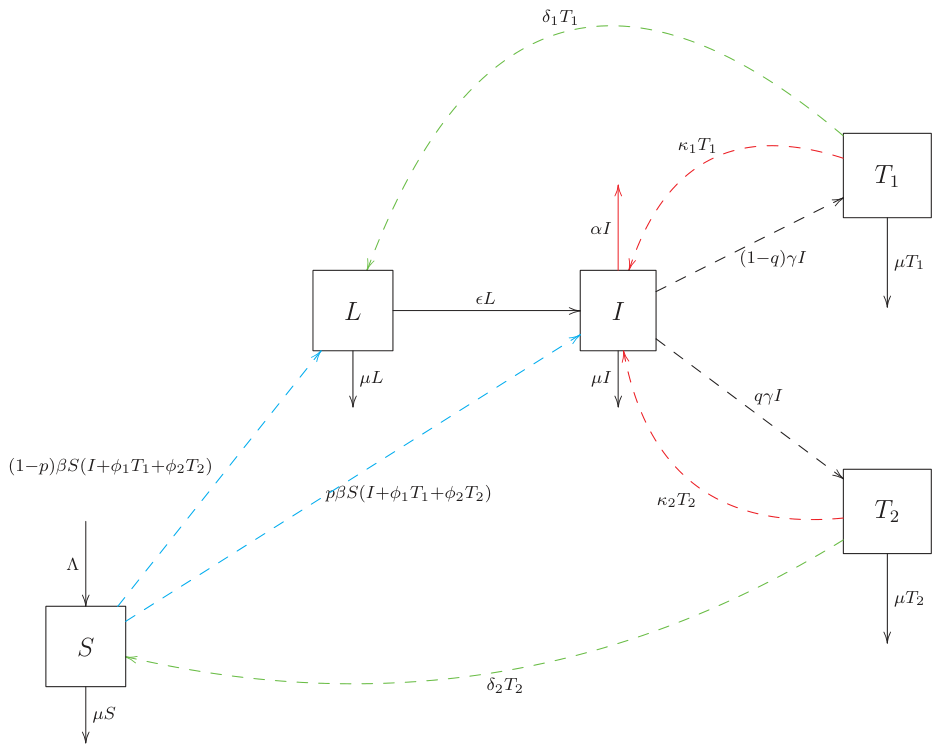
Figure 2.
Time-dependent function of relative cost defined by (23) and related to sterilizing treatment
Figure 2.
Time-dependent function of relative cost defined by (23) and related to sterilizing treatment
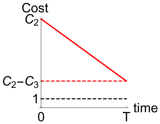
Figure 3.
Basic reproductive number as a function of
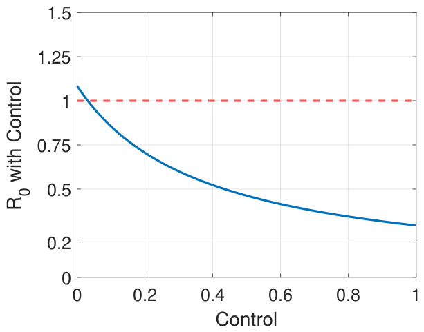
Figure 4.
Sobol2002 sensitivity indexes
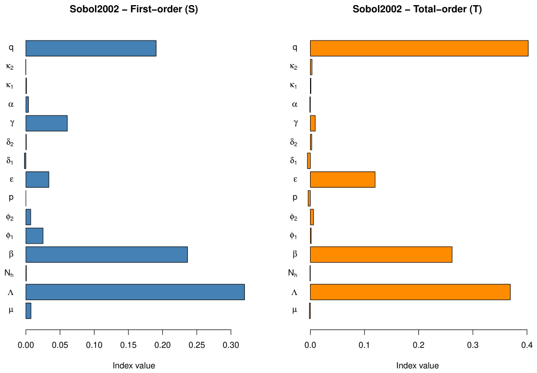
Figure 5.
Time evolution of latent and active TB infections, (left-hand chart) and (right-hand chart) for solely non-sterilizing (, blue-colored curves) and sterilizing (, red-colored curves) treatment.
Figure 5.
Time evolution of latent and active TB infections, (left-hand chart) and (right-hand chart) for solely non-sterilizing (, blue-colored curves) and sterilizing (, red-colored curves) treatment.
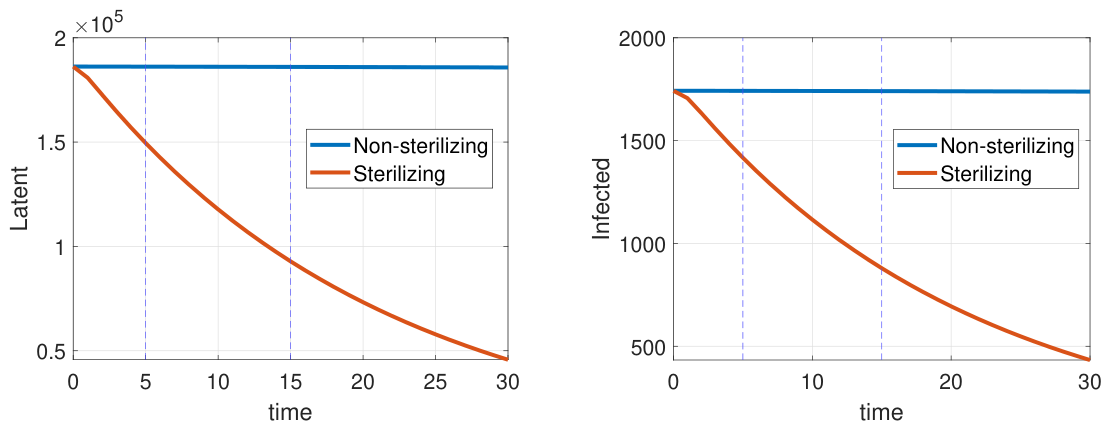
Figure 6.
Cumulative latent TB infections, (upper left chart), cumulative active TB infections, (upper right chart), and cumulative TB-induced mortality, (bottom row) for solely non-sterilizing (, blue-colored curves) and sterilizing (, red-colored curves) treatment.
Figure 6.
Cumulative latent TB infections, (upper left chart), cumulative active TB infections, (upper right chart), and cumulative TB-induced mortality, (bottom row) for solely non-sterilizing (, blue-colored curves) and sterilizing (, red-colored curves) treatment.
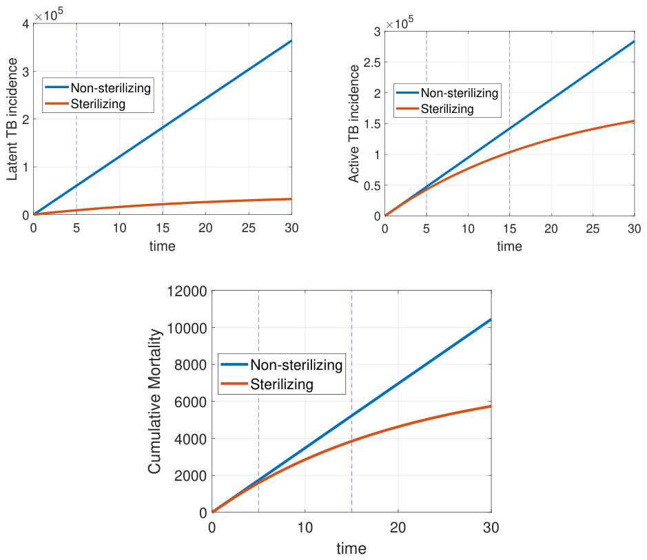
Figure 7.
Illustration of the decreasing cost functions and with (left chart) and (right chart) and with underlying values of for each that are compatible with the formulas (23), (25)
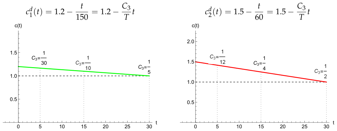
Figure 8.
Cumulative costs related to constant relative cost (, left chart) and decreasing relative cost (, right chart).
Figure 8.
Cumulative costs related to constant relative cost (, left chart) and decreasing relative cost (, right chart).
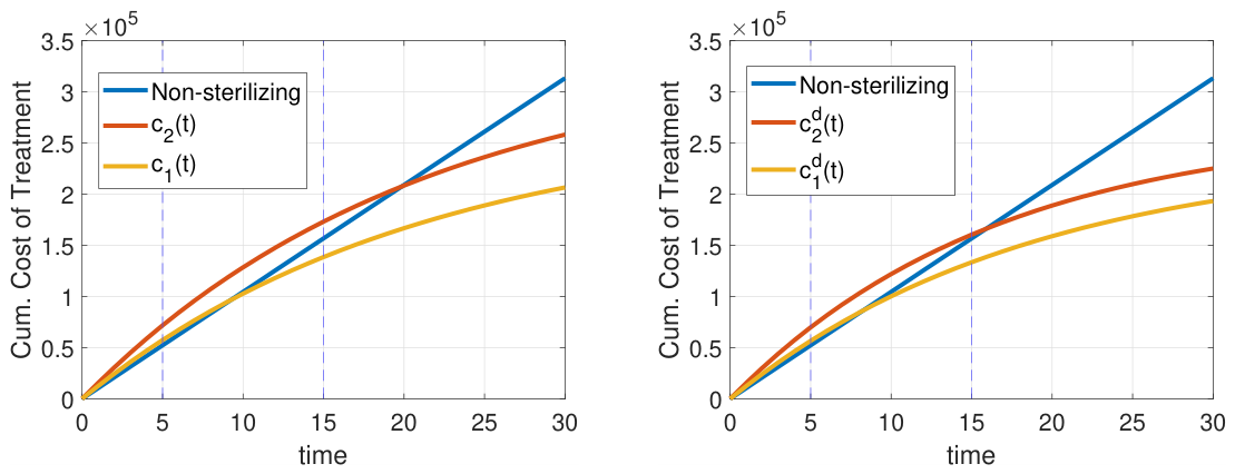
Figure 9.
Optimal bang-bang controls (left column) and the corresponding switching functions (right column).
Figure 9.
Optimal bang-bang controls (left column) and the corresponding switching functions (right column).
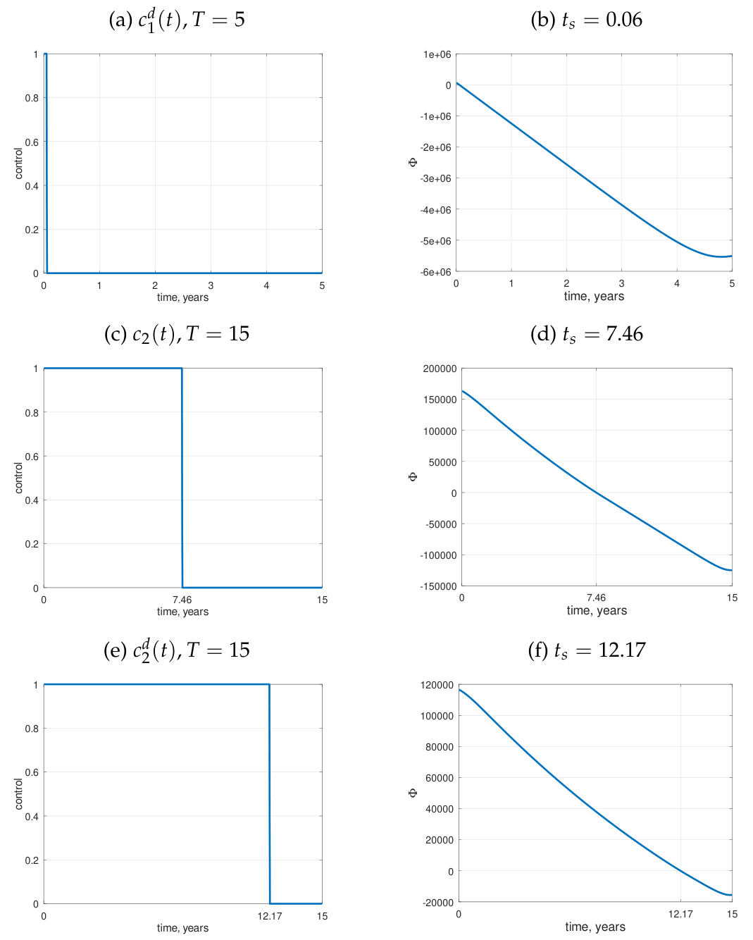
| (a) | (b) | |
| (c) | (d) | |
| (e) | (f) | |
Figure 10.
Estimated benefits and cumulative extra costs corresponding to solely sterilizing treatment and bang-bang optimal control strategies in the short-term perspective, years
Figure 10.
Estimated benefits and cumulative extra costs corresponding to solely sterilizing treatment and bang-bang optimal control strategies in the short-term perspective, years
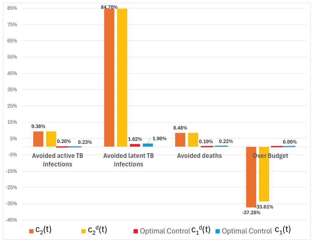
Figure 11.
Estimated benefits and cumulative extra costs corresponding to solely sterilizing treatment and bang-bang optimal control strategies in the medium-term perspective, years
Figure 11.
Estimated benefits and cumulative extra costs corresponding to solely sterilizing treatment and bang-bang optimal control strategies in the medium-term perspective, years
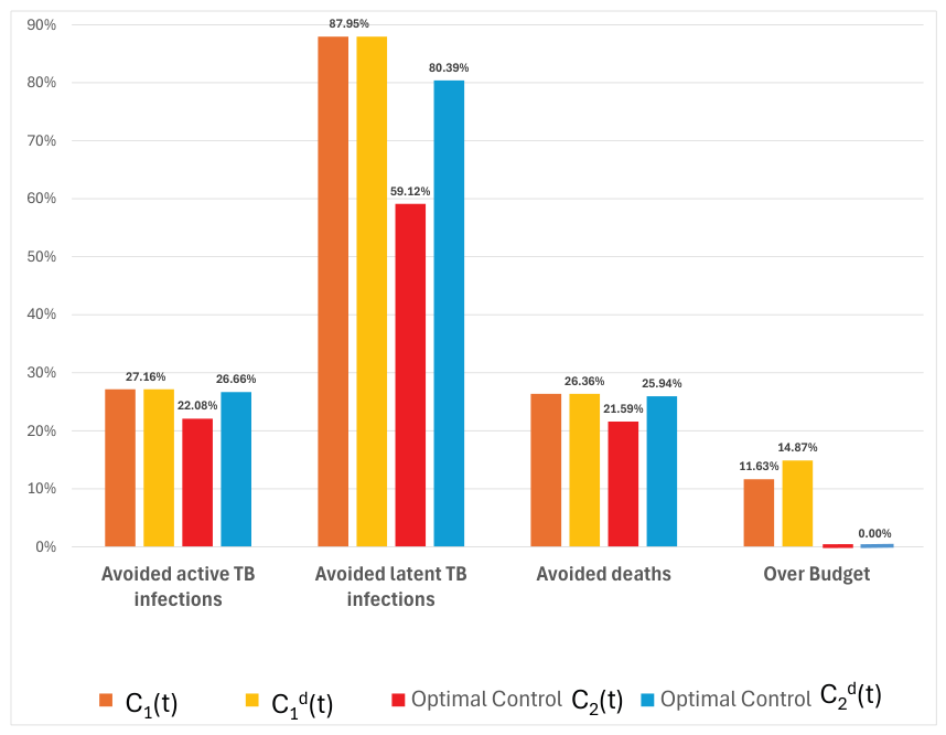
Figure 12.
Estimated benefits and potential savings corresponding to solely sterilizing treatment in the long-term perspective, years.
Figure 12.
Estimated benefits and potential savings corresponding to solely sterilizing treatment in the long-term perspective, years.
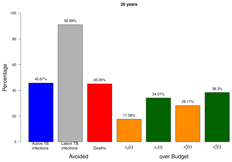

Table 1.
Description of the parameters of the model (2)
| Parameter | Description | Units |
|---|---|---|
| Recruitment of individuals | person × time−1 | |
| Natural mortality rate | time−1 | |
| TB-induced mortality rate | time−1 | |
| TB transmission rate | (person × time)−1 | |
| Reduction of the infectiousness by non-sterilizing | dimensionless | |
| treatment () or sterilizing treatment () | ||
| p | Fraction of direct progression to active infections | dimensionless |
| q | Fraction of patients assigned for sterilizing treatment | dimensionless |
| Rate of development of slow TB infections | time−1 | |
| Completion rate of non-sterilizing and | time−1 | |
| sterilizing treatment | ||
| Treatment recruitment rate | time−1 | |
| Abandonment rate of non-sterilizing and | time−1 | |
| sterilizing treatment |
Table 2.
Numerical values of parameters of the dynamical systems (2), (Section 4); time is measured in years
Table 2.
Numerical values of parameters of the dynamical systems (2), (Section 4); time is measured in years
| Parameter | Value | Range | References/Comments |
|---|---|---|---|
| fitted | |||
| [25] | |||
| fitted | |||
| [3,8,9,26] | |||
| p | [27,28,29] | ||
| [4,30,31] | |||
| 2 | [4,31] | ||
| 6 | [4] | ||
| [27,31] | |||
| [7,30,32] | |||
| varied | — |
Table 3.
Short-, medium-, and long-term performance of sterilizing versus non-sterilizing treatment
| Indicator | Sterilizing treatment, | Non-sterilizing treatment, | ||||
|---|---|---|---|---|---|---|
|
Short |
Medium |
Long |
Short |
Medium |
Long |
|
| Cumulative active infections | 42930 | 103482 | 154288 | 47372 | 142072 | 283975 |
| Cumulative latent infections | 9306 | 21974 | 32846 | 60824 | 182384 | 364471 |
| Cumulative mortality | 1595 | 3848 | 5739 | 1742 | 5225 | 10444 |
| Total No. of treatments started | 47836 | 115441 | 172160 | 52268 | 156758 | 313331 |
| Total No. of treatment dropouts | 6297 | 15241 | 22743 | 6772 | 20311 | 40599 |
| Total No. of treatment completions | 41982 | 101606 | 151620 | 45150 | 135409 | 270660 |
Table 4.
Prices for TB drugs in US dollars borrowed from [16]
Table 4.
Prices for TB drugs in US dollars borrowed from [16]
| Drug | Dose per tablet |
Lower bound (USD) |
Upper bound (USD) |
Average (USD) |
Tablets per daily dose |
Intensive phase (days) |
Continuation phase (days) |
Total cost per treatment |
|---|---|---|---|---|---|---|---|---|
| Isoniazid (H) | 300 mg | 0.02 | 0.19 | 0.105 | 1 (300 mg) | 60 | 120 | 18.90 |
| Rifampicin (R)* | 600 mg | 0.66 | 2.45 | 1.555 | 1 (600 mg) | 60 | 120 | 279.90 |
| Pyrazinamide (Z)* | 500 mg | 0.02 | 0.90 | 0.46 | 4 (2000 mg) | 60 | 0 | 110.40 |
| Ethambutol (E) | 400 mg | 0.04 | 0.31 | 0.175 | 3 (1200 mg) | 60 | 0 | 31.50 |
*Drugs bearing the sterilizing effect.
Table 5.
Cumulative costs for solely non-sterilizing and solely sterilizing treatment
| Treatment type | Short-term, | Medium-term, | Long-term, |
|---|---|---|---|
| years | years | years | |
| Non-sterilizing | 52 268 | 156 758 | 313 331 |
| Sterilizing with constant cost | 57 138 | 138 530 | 206 592 |
| Sterilizing with constant cost | 71 753 | 173 162 | 258 240 |
| Sterilizing with decreasing cost | 56 636 | 133 441 | 193 320 |
| Sterilizing with decreasing cost | 69 836 | 160 631 | 225 095 |
Table 6.
Type of optimal control obtained for different cost functions
| Cost function | Short-term, | Medium-term, | Long-term, |
|---|---|---|---|
| years | years | years | |
| Constant lower cost | bang-bang | ||
| Constant higher cost | bang-bang | ||
| Decreasing lower cost | bang-bang | ||
| Decreasing higher cost | bang-bang |
Table 7.
Short- and medium-term performance of optimal control strategies
| Indicator | Short-term, years | Medium-term, years | ||
|---|---|---|---|---|
| Constant cost | Decreasing cost | Constant cost | Decreasing cost | |
| Cumulative active infections | ||||
| Cumulative latent infections | ||||
| Cumulative mortality | ||||
| Total no. of treatments started | ||||
| Total no. of treatment dropouts | ||||
| Total no. of treatment completions | ||||
Disclaimer/Publisher’s Note: The statements, opinions and data contained in all publications are solely those of the individual author(s) and contributor(s) and not of MDPI and/or the editor(s). MDPI and/or the editor(s) disclaim responsibility for any injury to people or property resulting from any ideas, methods, instructions or products referred to in the content. |
© 2026 by the authors. Licensee MDPI, Basel, Switzerland. This article is an open access article distributed under the terms and conditions of the Creative Commons Attribution (CC BY) license.
Copyright: This open access article is published under a Creative Commons CC BY 4.0 license, which permit the free download, distribution, and reuse, provided that the author and preprint are cited in any reuse.