
Submitted:
02 July 2026
Posted:
03 July 2026
You are already at the latest version
Abstract
Fine-grained and open-set fault diagnosis of analog circuits poses two challenges that generic deep classifiers fail to address. First, under a closed-set assumption, models assign unseen fault types to known classes with unwarranted confidence, lacking any mechanism to reject out-of-distribution inputs. Second, component manufacturing tolerances induce structured intra-class variation that causes the frequency responses of distinct fault modes to overlap, severely degrading fine-grained discrimination. This paper proposes a Tolerance-Aware Contrastive Siamese Network (TCSN), a metric-learning framework that constructs a discriminative embedding space jointly addressing both issues. The core contribution is the Tolerance-Aware Contrastive Loss (TACL), comprising a tolerance term \( (\mathcal{L}_{\mathrm{tol}}) \) that suppresses tolerance-induced intra-class scatter across Monte Carlo realizations, and a fine-grained term \( (\mathcal{L}_{\mathrm{fg}}) \) that enforces separation of near-identical overlapping classes. For open-set rejection, an energy-based scoring mechanism maps prototype distances into in-/out-of-distribution scores, identifying unknown faults without retraining. The framework is validated on a Sallen-Key second-order Butterworth low-pass filter benchmark (10 known and 2 unknown fault classes). It attains an open-set AUROC of 0.9309 and an FPR@95%TPR of 0.2500; for closed-set classification it reaches 90% accuracy (macro-F1: 0.88), and it retains 83.0% accuracy under one-shot conditions (n = 1). Under corrupted inputs it degrades gracefully, outperforming all baselines at 10 dB SNR. Ablations confirm the necessity of each component: removing \( \mathcal{L}_{\mathrm{tol}} \) drops the open-set AUROC by 0.3793, removing \( \mathcal{L}_{\mathrm{fg}} \) reduces fine-grained accuracy by 11 percentage points, and replacing energy scoring with distance thresholding lowers the AUROC by 0.2683.
Keywords:
contrastive learning
; metric learning
; open-set recognition
; few-shot learning
; out-of-distribution detection
; energy score
; Siamese network
; analog circuit fault diagnosis
1. Introduction
Fault diagnosis of analog circuits remains a long-standing problem in reliability engineering, as analog components form the critical interface between the physical world and digital signal processing in virtually every electronic system [1,2]. Unlike digital circuits, whose faults are typically binary and localized, analog faults are inherently parametric and highly coupled, producing a continuum of overlapping signatures that is difficult to separate. Early diagnostic methodologies relied on signal processing and analytical modeling, such as combining wavelet transforms with neural networks for feature extraction [3,4], Volterra series and subband decomposition for nonlinear parametric faults [5], and dependence matrices with intelligent classifiers to narrow ambiguous fault groups [4,6]. While effective, these techniques rely on manually engineered features whose adaptability is limited under increasingly complex integration scales [7].
To overcome the limitations of manual feature engineering, deep learning has been widely adopted to process high-dimensional response signals directly [8,9]. Recent studies demonstrate the efficacy of deep generative models [10] and self-supervised contrastive learning via 1D-CNNs [11] in capturing nonlinear fault signatures, and related architectures such as Signal-Transformers [12], decoupled CNNs [13], and transfer-learning schemes [14,15] have advanced fault diagnosis across broader domains. However, a critical vulnerability persists: most of these data-driven models operate under a strict closed-set assumption.
From a learning perspective, this continuum of fault manifestations creates two fundamental challenges that existing methods fail to fully address:
First, open-set recognition. In practice it is infeasible to collect labeled samples for all possible fault states prior to deployment [16]. Novel, unseen faults inevitably occur, and a reliable model must detect and reject such “unknown” inputs rather than overconfidently misclassifying them into known classes, which leads to fatal false positives [17]. Designing a decision metric that detects unseen anomalies without retraining is imperative yet challenging.
Second, fine-grained ambiguity induced by tolerances. Component manufacturing tolerances introduce structured intra-class variation that corrupts the underlying correlation structure of the data [18], requiring nonlinear quantification [19]. Tolerances distort nominal signal trajectories, causing severe intra-class scatter and inter-class overlap between distinct fault modes (e.g., a deviation of vs. ). Although early efforts handled tolerance via slope fault models and test-point selection [20], decoupling tolerance-induced metric distortion from genuine fault patterns within a deep embedding space remains unresolved.
Rather than adapting a generic classifier or a standard anomaly score [21,22,23], this paper proposes a Tolerance-Aware Contrastive Siamese Network (TCSN), an end-to-end metric-learning framework tailored to the structured variability of analog faults. TCSN learns a discriminative embedding space that simultaneously resolves tolerance-induced ambiguity, operates effectively with limited samples, and reliably detects unseen anomalies under noisy conditions.
The main contributions of this work are summarized as follows:
- 1.
- Tolerance-Aware Contrastive Loss (TACL). We propose a metric-learning objective tailored to structured tolerance variation. The tolerance term () suppresses intra-class scatter by pulling Monte Carlo tolerance realizations toward a stable reference prototype, while the fine-grained term () enforces separation of nearly identical overlapping classes. Ablations confirm the necessity of this design: omitting degrades open-set AUROC by 0.3793, while omitting reduces closed-set accuracy by 11 percentage points.
- 2.
- Energy-based open-set rejection. We introduce a calibration-free decision mechanism for open-set recognition. By adapting the energy score to a prototype-based metric space, the model maps embedding distances into reliable in-/out-of-distribution scores, identifying unknown faults and achieving an AUROC of 0.9309 and an FPR@95%TPR of 0.2500, outperforming distance-based rejection by 0.2683 in AUROC.
- 3.
- End-to-end representation learning from raw responses. The framework operates directly on 401-point log-magnitude frequency responses, eliminating fragile handcrafted feature extraction. The encoder produces robust embeddings that remain resilient to additive noise.
- 4.
- Comprehensive evaluation. TCSN is validated on a representative Sallen-Key Butterworth filter benchmark (10 known and 2 unknown classes). It achieves 90% closed-set accuracy, outperforms all baselines under limited data (), maintaining 83.0% accuracy at , and degrades gracefully under 10–30 dB SNR noise where traditional methods collapse.
2. Related Work
2.1. Analog Circuit Fault Diagnosis
Early fault diagnosis methods constructed fault dictionaries and matched measured responses to pre-computed signatures [1]. Subsequent approaches extracted features such as wavelet coefficients, pole-zero locations, and frequency-domain moments, then applied classical classifiers including support vector machines [20,24] and neural networks [3,4,25]. These methods require domain expertise for feature design and are sensitive to component-tolerance variation that shifts feature distributions [7,26]. Parametric fault localization techniques address tolerance explicitly via sensitivity analysis, but their scalability to high-dimensional response data remains limited [5,6].
More recently, deep learning methods have achieved state-of-the-art closed-set accuracy on analog fault benchmarks. CNN-based methods applied directly to time- or frequency-domain signals eliminate manual feature engineering and learn hierarchical representations [8,27,28]. Generative adversarial networks and attention-augmented networks have further improved feature discrimination for soft fault diagnosis [10,29,30]. However, these supervised classifiers require large labeled datasets and cannot detect unknown faults at test time [31]—gaps that TCSN addresses via metric learning and energy-based detection.
2.2. Metric Learning and Few-Shot Diagnosis
Metric learning trains an embedding function such that semantically similar samples are close and dissimilar samples are far in a learned distance space [21,32,33]. Siamese networks [34] learn pairwise similarity using contrastive loss [33], and prototypical networks [21] extend this to multi-class few-shot recognition via nearest-prototype classification.
These frameworks have been extensively validated in fault diagnosis of complex industrial equipment and rotating machinery [12,35,36], where decoupling highly overlapping fault signatures is paramount [13], demonstrating strong generalization from limited labeled data. A recent contrastive learning approach for analog circuit soft fault diagnosis further validates the applicability of metric learning to this domain [11]. TCSN extends this line of work by incorporating a tolerance-specific regularization term that accounts for the structured intra-class variability induced by manufacturing tolerances—a challenge absent in typical image or vibration benchmarks [37,38].
2.3. Open-Set Recognition and Out-of-Distribution Detection
Open-set recognition requires a model to detect inputs belonging to classes unseen during training, rather than force-classifying them into known categories [17]. Threshold-based methods on softmax scores suffer from overconfidence on out-of-distribution inputs [39]. More principled approaches include reconstruction-based anomaly detection, density estimation, and Bayesian uncertainty quantification via MC Dropout [40]. The energy score [22] provides a logit-based alternative that requires no calibration and has shown strong empirical performance across vision benchmarks.
In the fault diagnosis domain, open-set detection has received limited attention, and most existing works assume a closed-world setting where all test faults belong to known classes [16,23,41,42]. TCSN fills this gap by adapting the energy score to a prototype distance space, achieving reliable open-set detection without sacrificing closed-set classification performance.
2.4. Component Tolerance Modeling
Component manufacturing tolerances introduce continuous variation into circuit parameters, causing nominally identical circuits to exhibit measurable response variation [7,37]. Monte Carlo simulation is the standard tool for quantifying this variability [38], and its application to fault diagnosis data generation has been demonstrated in prior works [4,5].
However, most existing methods treat tolerance purely as noise to be filtered rather than a structural property to be modeled. Quantifying and handling such intrinsic uncertainty is crucial for reliable decision-making [18]. TCSN instead explicitly incorporates tolerance variation through MC-augmented training data and the regularization term, turning tolerance variability into a structural prior that improves embedding robustness.
3. Circuit Model and Fault Formulation
As illustrated in Figure 1, the proposed framework bridges signal acquisition with deep metric learning. To formulate the task, this section details the analog circuit model, the fault space definitions, and the quantification of structural uncertainties.
3.1. Sallen-Key Filter Topology
The Sallen-Key second-order Butterworth low-pass filter is adopted as the circuit under test, owing to its widespread use in signal conditioning and its sensitivity to parametric variations [2,6]. As shown in Figure 2, the circuit comprises two resistors (, ), two capacitors (, ), and a voltage-follower amplifier with gain-setting resistors and .
The nominal component values and resulting filter parameters are listed in Table 1. With , , , and , the theoretical cutoff frequency and quality factor are calculated by:
where is the amplifier gain. Circuit simulation in Multisim yields a nominal cutoff frequency of . The simulation output exhibits a maximum deviation from the theoretical transfer function of only (RMS: ). This extremely low residual error provides a reliable baseline for subsequent uncertainty modeling, as illustrated in Figure 3.
3.2. Fault Class Definition
Twelve circuit states are defined, comprising ten known classes (F0–F9) used for training and closed-set testing, and two unknown classes (U1, U2) reserved exclusively for open-set evaluation. Table 2 provides the complete fault catalog.
Known faults span four categories: (i) the nominal class F0; (ii) single resistor deviations (F1–F6) ranging from to ; (iii) single capacitor deviations (F7, F8) at ; and (iv) one hard open-circuit fault (F9, replaced by ). The unknown faults simulate unforeseen anomalies, including a compound fault U1 ( simultaneously with ) and a large-deviation fault U2 (), both of which fall strictly outside the distribution of training data.
3.3. Fine-Grained Fault Similarity Analysis
Figure 4 illustrates the frequency responses of all ten known classes overlaid on the nominal response. While most faults produce measurable frequency shifts, certain analogous pairs—notably F1 () and F3 ()—exhibit profound spectral overlaps that are highly challenging to decouple by standard heuristic observation. This high inter-class similarity constitutes a primary challenge for conventional diagnostic algorithms.
To quantitatively assess this diagnostic difficulty, we compute the cosine similarity between the nominal frequency-response vectors of each fault pair, as reported in Figure 5.
The analysis indicates that the F0–F8 classes are highly coupled in the raw frequency-response space, with pairwise cosine similarities ranging from 0.998 to 0.9999. The most challenging pairs are F1–F3 ( vs. , similarity ) and F3–F8 ( vs. , similarity ), demonstrating that parametric deviations in different components can manifest as nearly identical signatures. By contrast, F9 ( open circuit) is structurally separated from other classes, with pairwise similarities of 0.922–0.941, consistent with its distinct early roll-off behavior. These near-degenerate pairs highlight the critical necessity of the fine-grained loss term introduced later in Section 5.
3.4. Monte Carlo Tolerance Simulation
Component manufacturing tolerances introduce inherent uncertainty into the circuit parameters. To model this structural variability, Monte Carlo (MC) simulation is applied. For each defined class, instances are generated by independently sampling each component value from a uniform distribution centered on its nominal (or faulted) value, with tolerance for resistors and for capacitors:
where is the center value of the k-th component and [7,37].
The resulting distribution of the normal-class cutoff frequency is (coefficient of variation CoV = 2.95%), indicating that tolerance-induced uncertainty is non-negligible relative to inter-class deviations. Crucially, the F1 fault () produces a nominal shift of only from the normal-class distribution, classifying it as a marginal fault that is highly susceptible to misclassification under standard scalar-based thresholding.
However, the complete 401-point frequency-response vector retains subtle spectral discrepancies that are difficult to capture via scalar feature extraction. As quantified in Section 3-C, even the most overlapping fault pairs remain theoretically distinguishable in the high-dimensional space, suggesting that multivariate metric learning is highly suitable for this fine-grained task.
3.5. Frequency Response Acquisition
The AC frequency response for each MC instance is acquired over the range at 401 logarithmically spaced frequency points, yielding the magnitude response vector:
This raw sequence serves directly as the input to the deep learning model after standard z-score normalization (detailed in Section 5-A), bypassing manual feature engineering [8]. The selected resolution of 401 points provides sufficient spectral fidelity to distinguish fault pairs with extreme cosine similarities, laying the data foundation for the subsequent TCSN framework.
4. Data Generation and Dataset Construction
4.1. Simulation and Acquisition Pipeline
The dataset is constructed through an automated pipeline implemented in Python, interfacing with Multisim via COM automation. For each fault class and each Monte Carlo trial, the pipeline executes the following procedures: (i) sample component values according to (3); (ii) inject the sampled values into the Multisim netlist; (iii) perform an AC sweep over at 401 logarithmically spaced frequency points; (iv) export the magnitude response in the linear scale; and (v) convert the magnitudes to decibels to form the input vector.
To simulate inherent noise during acquisition and evaluate model robustness (subsequently discussed in Section 6-E), additive white Gaussian noise is introduced. Crucially, this noise injection is applied in the linear domain prior to decibel conversion, thereby preserving the physical interpretation of the Signal-to-Noise Ratio (SNR):
where and the clipping operation is employed to prevent non-physical negative magnitudes. This MC-based simulation methodology aligns with established benchmark practices for analog circuit fault diagnosis [43].
4.2. Dataset Splits
The complete dataset comprises samples (10 known classes × 100 samples + 2 unknown classes × 50 samples each). The allocation of these samples is detailed in Table 3.
Stratified sampling is utilized to ensure that the class distribution of the tolerance-induced variations is consistently maintained across the splits. The unknown subset is kept strictly disjoint from all training and validation data, being accessed exclusively during the final open-set evaluation phase.
4.3. Input Normalization
The raw dB-domain frequency responses are standardized utilizing the statistical parameters derived solely from the training set:
where and represent the per-frequency-point mean and standard deviation computed over the training set, respectively, and is added for numerical stability. Validation, test, and unknown samples are normalized using these same training-set statistics. This approach reflects practical scenarios where prior knowledge of the test data distribution is typically unavailable [31].
4.4. Data Integrity Verification
To ensure methodological rigor and verify the absence of unintended data leakage, a label-shuffle test is conducted. Specifically, the training labels are randomly permuted while keeping the input features unchanged, after which the proposed model is retrained from scratch. The resulting test accuracy drops to , which is consistent with the random guessing baseline for a 10-class classification problem (). This result confirms that the model relies entirely on the structural information embedded in the features, rather than memorizing spurious correlations.
4.5. Tolerance-Induced Variability Analysis
Figure 6 illustrates the Monte Carlo (MC) tolerance envelope of the nominal state, with representative marginal and structural fault responses overlaid for comparative analysis.
The standard deviation of the nominal-class cutoff frequency across MC trials is (mean: , CoV = 2.95%), demonstrating that tolerance-induced uncertainty is comparable in magnitude to the inter-class frequency shifts caused by marginal faults.
The severity of tolerance-induced overlap between adjacent fault classes can be quantitatively characterized by the normalized distance between the mean of class c and the normal class in a given scalar feature k. As explicitly demonstrated in Figure 6(b), the marginal fault F1 is located at from the nominal distribution. This proximity places it firmly within the typical tolerance band, rendering conventional scalar-feature thresholding highly susceptible to misclassification.
By contrast, the structural fault F9 ( open circuit) exhibits cosine similarities of only 0.922–0.941 with all other classes (as established in Figure 5), indicating that it is structurally separated and readily diagnosable. This extreme variance in diagnostic difficulty—ranging from heavily coupled marginal deviations (e.g., F1) to clearly distinct structural anomalies (e.g., F9)—provides the precise motivation for the multi-scale contrastive training strategy detailed subsequently. By leveraging both hard and easy fault pairs, the proposed strategy can appropriately shape the feature embedding space to decouple these overlapping distributions [21,33].
5. Proposed TCSN Framework
This section presents the Tolerance-Aware Contrastive Siamese Network (TCSN), a unified framework designed for the isolation of subtle parametric analog circuit faults and the open-set detection of unknown anomalies. As illustrated in Figure 7, the TCSN architecture comprises three primary modules: (i) a 1D-CNN encoder that extracts discriminative embeddings directly from raw frequency-response inputs; (ii) a Tolerance-Aware Contrastive Loss (TACL) that explicitly accounts for the uncertainty induced by component tolerances; and (iii) an energy score module configured for the open-set detection of previously uncharacterized faults.
5.1. Input Representation
In contrast to conventional methods that rely on the extraction of pre-defined features (e.g., cutoff frequency or quality factor) [4,24], TCSN operates directly on the raw log-magnitude frequency response. For each circuit under test (CUT), the frequency response is acquired over the range of at 401 logarithmically spaced points, yielding an observation vector in decibels. The input is standardized as follows:
where and denote the per-channel mean and standard deviation computed over the training set. This data-driven formulation mitigates the subjective biases introduced by manual feature selection and enables the network to automatically discover patterns highly sensitive to circuit degradation.
5.2. 1D-CNN Encoder
The encoder is designed to map the high-dimensional input vector to a compact, unit-norm embedding space. It incorporates three strided 1D convolutional blocks followed by two fully connected layers, with the structural specifics detailed in Table 4.
Design rationale. Layer normalization (LayerNorm) [44] is intentionally utilized instead of batch normalization to support single-sample inference (). This property is critical for few-shot scenarios where the support data may be severely limited. The final L2 normalization layer projects the embeddings onto a unit hypersphere, ensuring that Euclidean distance mathematically aligns with cosine similarity. This establishes a strictly bounded geometric space for prototype matching and energy score computation. Dropout () is applied after each convolutional block and the first fully connected layer to prevent overfitting given the limited sample sizes.
5.3. Tolerance-Aware Contrastive Loss (TACL)
5.3.1. Motivation
In practical circuits, inherent manufacturing tolerances cause frequency-response samples of the same fault class to exhibit a continuous scatter rather than converging to a deterministic point. Standard contrastive losses treat all intra-class pairs symmetrically, failing to exploit this statistical variability. Consequently, it becomes challenging for the model to decouple tolerance-induced deviations from genuine fault-induced signal shifts. TACL addresses this issue by integrating a tolerance regularization term that enforces intra-class compactness, alongside a fine-grained repulsion term that explicitly segregates highly coupled fault classes whose signatures are nearly identical.
5.3.2. Loss Formulation
The comprehensive training objective is formulated as:
with the weighting coefficients , , and empirically determined via grid search on the validation set.
Contrastive loss . Following the Siamese network paradigm [33], pairs of embeddings are constructed within each mini-batch. Let if the pair belongs to the same fault class, and otherwise. Defining the Euclidean distance as , the loss is computed as:
where represents the contrastive margin and denotes the set of all pairs in the current batch.
Tolerance regularization . For each defined fault class c, let represent the mean embedding of all training samples assigned to c. The tolerance term is designed to minimize the intra-class scatter:
where C is the total number of known fault classes and denotes the index set of class c. This regularization forces the encoder to map Monte Carlo tolerance realizations into a dense spherical cluster, thereby establishing a stable reference prototype for subsequent evaluations [37].
Fine-grained loss . As quantitatively established in Section 3, certain fault configurations produce highly overlapping raw vectors. Specifically, the pairs F1–F3 ( vs. ) and F3–F8 ( vs. ) yield raw cosine similarities of and , respectively. Such highly coupled characteristics constitute hard negative samples that alone cannot robustly separate. The fine-grained term introduces an amplified repulsion gradient for these specific pairs:
where encompasses the set of cross-class hard pairs whose raw similarity exceeds the threshold , and is an expanded margin parameter. Subsequent ablation studies (Section 6-F) verify that omitting results in an 11-percentage-point degradation in closed-set accuracy (from 90% to 79%).
5.4. Prototype-Based Classification
Upon completion of the training phase, an anchor prototype is calculated for each class as the geometric centroid of its respective training embeddings:
During the inference stage, the diagnostic decision for a newly acquired query sample is formulated via nearest-centroid matching:
where represents the dictionary of predefined fault classes. A significant advantage of this prototype-based mechanism is that it inherently supports varying support-set sizes (n) without necessitating model retraining, facilitating flexible few-shot diagnosis under constrained conditions [21].
5.5. Energy Score-Based Open-Set Detection
5.5.1. Motivation
In practical scenarios, the system may encounter uncharacterized fault types, such as compound component degradation or out-of-distribution catastrophic failures. A robust framework must possess the capability to flag these anomalies rather than erroneously forcing them into a known category. To fulfill this requirement, we implement an energy score module [22] adapted for the prototype metric space. This method aggregates the distance distribution across all known classes to quantify epistemic uncertainty. Alternatively, MC Dropout was evaluated as a baseline for uncertainty estimation; however, it exhibited high variance on this compact 1D-CNN architecture, with the AUROC degrading to below 0.70 across various MC sampling counts (, as detailed in Table 10).
5.5.2. Energy Score Formulation
Given the predefined class prototypes , the deviation distance for a specific class c is defined as . The energy score, inspired by free energy concepts in out-of-distribution detection [22], is subsequently computed as:
where acts as a temperature scaling parameter. When the input closely aligns with a known prototype, the summation in (14) is dominated by a significantly large exponential component, returning a lower . Conversely, if diverges from all established prototypes, the terms diminish exponentially, and due to the leading negative sign, it results in a higher . The optimal temperature coefficient was established by maximizing the AUROC performance on the validation dataset across the grid .
5.5.3. Detection Decision Logic
An input is identified as an unknown fault if its calculated energy score exceeds a specified operational threshold :
The threshold is calibrated on the validation set targeting a 95% True Positive Rate (TPR) operating point, which empirically yielded a False Positive Rate (FPR@95%TPR) of .
5.6. Training Strategy
The TCSN framework is optimized via a two-phase training protocol. During Phase 1 (spanning 200 epochs, inclusive of 10 warm-up epochs), only the standard contrastive loss is activated. This initialization establishes a stable metric-space topology before the introduction of the more complex tolerance and fine-grained constraints [45]. The learning rate undergoes a linear warm-up from 0 to . In Phase 2 (spanning 300 epochs), the complete objective function comprising all three loss components is activated, and the network is fine-tuned until the validation accuracy plateaus at 94%. The optimization is executed using the Adam algorithm with a weight decay of . Mini-batches of size 128 are employed, coupled with online hard-negative mining to accelerate convergence. To ensure the strict reproducibility of the reported results, a constant global random seed of 42 is maintained across all experiments.
6. Experiments and Results
6.1. Experimental Setup
6.1.1. Circuit Under Test (CUT) and Data Acquisition
All experiments are conducted using a Sallen-Key second-order Butterworth low-pass filter, a standard benchmark circuit for analog fault diagnosis, simulated via Multisim [2]. The nominal specifications of the components are defined as , , , and . This configuration yields a theoretical cutoff frequency of and a quality factor of .
To evaluate the framework, ten distinct health states are defined (designated as F0–F9), comprising one nominal state, eight parametric deviations (single-component degradation), and one catastrophic open-circuit fault (detailed in Table 2). Additionally, two out-of-distribution (OOD) scenarios representing uncharacterized compound faults (U1, U2) are generated exclusively for open-set detection evaluation; these are strictly withheld during the training phase.
To emulate the statistical variability inherent in physical systems due to manufacturing tolerances and environmental drifts, Monte Carlo (MC) analysis is employed. Component values are sampled from uniform distributions ( for resistors, for capacitors). For each MC realization, an AC frequency sweep is performed from to at 401 logarithmically spaced frequency points. This procedure yields an input vector in decibels, which is subsequently standardized to zero mean and unit variance based on the training-set statistics, as formulated in (7).
The generated dataset is partitioned into Train, Validation, Test, and Unknown sets containing 300, 100, 100, and 100 samples, respectively (where the Unknown set comprises 50 samples each of U1 and U2). To rigorously verify the absence of data leakage and confirm that the model learns genuine physical fault signatures rather than dataset artifacts, a label-shuffle test was executed: training the network with randomly permuted labels yielded an accuracy of approximately 8% (chance level), confirming strict data integrity.
6.1.2. Baseline Methods
To benchmark the proposed framework, four classical data-driven algorithms are evaluated: Support Vector Machine (SVM) utilizing a Radial Basis Function (RBF) kernel (, gamma=scale), k-Nearest Neighbors (KNN, ), Random Forest (RF, 100 estimators), and a Multi-Layer Perceptron (MLP, featuring hidden layers of 128 and 64 neurons). To ensure a strictly fair comparison and to exclude any bias introduced by manual feature engineering, all baseline models ingest the exact same standardized 401-dimensional frequency-response vectors as the proposed TCSN.
6.1.3. Implementation Details
The proposed TCSN framework is implemented within the PyTorch ecosystem. Benefiting from the highly compact nature of the 1D-CNN design, the framework demands minimal computational overhead, allowing both the training and inference phases to be efficiently executed on standard computational platforms (e.g., a standard personal computer) without the necessity for high-end specialized hardware accelerators.
The encoder architecture is configured with a fixed embedding dimensionality of and a dropout probability of . The optimization process strictly adheres to the two-phase training schedule detailed in Section 5-F. Phase 1 is executed for 200 epochs (incorporating 10 linear warm-up epochs) with only the standard contrastive loss activated. Phase 2 is subsequently conducted for an additional 300 epochs utilizing the comprehensive objective function [46].
Network parameters are updated using the Adam optimizer with a learning rate of and a weight decay coefficient of . Mini-batches of size 128 are employed, augmented with online hard-negative mining to facilitate efficient convergence. For the open-set detection module, the energy score temperature is maintained at , which was empirically selected via grid search over the set using the validation set. A constant global random seed of 42 is utilized across all experiments to guarantee strict reproducibility. The baseline classifiers are implemented using the scikit-learn library [47] and rely on default configurations unless specified otherwise.
6.1.4. Evaluation Metrics
The efficacy of the framework is assessed across multiple paradigms. Closed-set fault isolation performance is quantified using overall classification accuracy and per-class F1-scores (evaluated via macro- and weighted-averages). The performance of the open-set unknown anomaly detection is evaluated using the Area Under the Receiver Operating Characteristic Curve (AUROC) and the False Positive Rate at a 95% True Positive Rate (FPR@95%TPR), conforming to standard benchmarking protocols [17,48]. Furthermore, for few-shot scenarios, the reported accuracy metrics are averaged across five independent, randomized draws of the support set to mitigate sampling variance and ensure statistical robustness.
6.2. Closed-Set Fault Classification
6.2.1. Main Results
Table 5 details the closed-set fault isolation performance evaluated on the independent test set. The proposed TCSN framework achieves an overall test accuracy of 90% and a macro-F1 score of 0.88. Notably, the network demonstrates absolute precision (F1 = 1.00) in isolating catastrophic failures (e.g., the open-circuit condition in F9) and exhibits strong discriminative capability against various subtle parametric drifts (e.g., F5–F8).
The learning dynamics of the network, illustrated in Figure 8, further validate the efficacy of the proposed two-phase optimization strategy. As the training transitions from Phase 1 (pure contrastive learning) to Phase 2 (full TACL objective) at epoch 201, the validation accuracy swiftly ascends to a peak of 94% and subsequently stabilizes. This trajectory confirms sound convergence properties and demonstrates that the model does not manifest severe overfitting despite the presence of noise simulated by component tolerances.
6.2.2. Class-Specific Performance
Detailed class-specific evaluation reveals that seven out of the ten health states achieve F1-scores exceeding 0.85, with three classes (F6, F7, and F9) exhibiting perfect diagnostic precision (F1 = 1.00). These correspond to , , and the open-circuit fault, respectively. Their signatures are well-separated from other classes in the latent embedding space, a characteristic visually corroborated by the t-SNE projection in Figure 9. Furthermore, this visualization previews the spatial isolation of unknown conditions, setting the stage for open-set evaluation.
The most challenging diagnostic scenario is presented by F3 (, F1 = 0.62). As quantitatively established in Section 3, F3, F1 (), and F8 () constitute an intrinsically difficult subset due to their extraordinarily high raw cosine similarities (0.999976 for F3-F1, and 0.999939 for F3-F8).
Crucially, while the proposed TCSN framework—empowered by the fine-grained loss —successfully mitigates what would otherwise be a severe cross-misclassification between F1 and F3 (as evidenced in Figure 10, true F3 is never misclassified as F1, and only 10% of true F1 leaks into F3), this fundamental physical resemblance still leaves F3 as the most vulnerable class. The residual difficulty manifests primarily as F3 being misclassified as F8 (20%) and concurrently receiving false positive predictions originating from F1 (10%).
Such extreme resemblance renders these classes practically indistinguishable without the explicit intervention of . The ensuing ablation study (Section 6-F) empirically confirms this dependency, revealing that discarding deteriorates the overall accuracy by 11 percentage points, triggering a diagnostic collapse specifically within this highly coupled F1-F3-F8 triplet.
6.2.3. Comparative Analysis with Baseline Classifiers
Table 6 compares the diagnostic accuracy of the proposed TCSN framework against the four data-driven baselines utilizing the full training dataset.
Under the ideal full-data regime (i.e., abundant labeled samples and high signal quality), RF (94.4%) and MLP (99.0%) surpass TCSN in raw closed-set classification accuracy. However, this expected outcome does not detract from the overarching advantage of the proposed framework, justified by three critical requirements intrinsic to practical scenarios:
First, TCSN is fundamentally architected as a metric-learning framework optimized simultaneously for few-shot generalization and open-set detection, rather than exclusively maximizing closed-set accuracy under data-rich conditions [31,49]. Section 6-C demonstrates that TCSN substantially outperforms all baselines when the available training set shrinks to extremely sparse regimes ( samples per class).
Second, baseline algorithms such as RF and MLP inherently lack open-set detection capabilities. They are geometrically constrained to assign every incoming sample to one of the predefined fault classes, regardless of its topological distance from the characterized training distribution. In stark contrast, TCSN achieves a remarkable AUROC of 0.9309 on the open-set task (detailed in Section 6-D), providing a safety-critical capability absent in traditional baselines.
Third, under realistic noisy conditions (Section 6-E), the performances of RF and MLP undergo severe degradation (e.g., at SNR, RF plummets from 94.4% to 10.6%, and MLP drops from 99.0% to 29.0%). Conversely, TCSN demonstrates high resilience, maintaining meaningful diagnostic accuracy across the tested SNR spectrum.
In summary, while the ideal full-data accuracy of TCSN remains competitive (within 4.4 percentage points of RF), its genuine contribution lies in offering a unified framework capable of handling data scarcity, unforeseen anomalies, and environmental noise concurrently—challenges where standard baselines catastrophically fail.
6.3. Few-Shot Fault Diagnosis
To rigorously evaluate the practical utility of the proposed TCSN framework under scenarios of severe data scarcity, we conduct a comprehensive few-shot fault diagnosis experiment. In this setup, the support set for each known health state is strictly constrained to samples. For each specific n, five independent trials are executed utilizing randomly sampled support sets, and the averaged diagnostic accuracy is reported. For a fair comparison, all baseline classifiers are completely retrained on identical support sets. The neighborhood hyperparameter for KNN is dynamically bounded to to prevent empty neighborhood anomalies at exceptionally small values of n.
Table 7 summarizes the quantitative results across different data regimes, with the corresponding performance trajectories visualized in Figure 11.
The empirical results reveal that TCSN dominates in the extreme data-scarcity regime, exhibiting particularly pronounced advantages under one-shot () and two-shot () configurations. At the ultimate limit of , TCSN attains an accuracy of 83.0%, outperforming SVM (75.0%), KNN (13.4%), RF (78.0%), and MLP (71.2%) by margins of 8.0, 69.6, 5.0, and 11.8 percentage points, respectively. At , the proposed network swiftly reaches 90.4%, maintaining a distinct lead over the second-best method (RF at 88.6%).
As the available labeled data expands (), highly parameterized discriminative models (i.e., RF and MLP) begin to overtake TCSN in raw accuracy [31,49]. This performance crossover is an expected phenomenon: models equipped with vast parameter capacities can explicitly construct fine-grained, non-linear decision boundaries when fed with ample training examples, whereas TCSN relies on fixed topological prototypes. However, the crossover point corresponds to data-rich regimes; in real-world analog circuit maintenance, acquiring dozens of samples per fault class via physical fault injection campaigns is highly cost-prohibitive, making the one-shot and two-shot superiority of TCSN exceptionally valuable.
The robust few-shot capability of TCSN fundamentally stems from two synergistic architectural decisions. First, the metric-learning-based prototype classifier necessitates zero retraining; the prototype for any given class is mathematically derived as the mean embedding of its n support samples, instantly yielding a well-defined geometric decision boundary even at [21,35]. Second, the application of TACL vigorously enforces intra-class compactness during the off-line training phase. Consequently, a prototype computed from merely a single noisy sample remains a highly reliable geometric anchor for the entire latent class distribution, effectively mitigating the stochastic variations induced by component tolerances.
6.4. Open-Set Unknown Fault Detection
6.4.1. Experimental Setup
The open-set detection capability of TCSN is evaluated by formulating a binary Out-of-Distribution (OOD) detection task. The test suite comprises 100 known-class samples (drawn from the closed-set test data, assigned label 0) and 100 unknown-class samples (assigned label 1). The unknown set intentionally incorporates two distinct types of anomalies to simulate realistic unforeseen failures: U1 contains 50 compound faults (simultaneous multi-component deviations), and U2 comprises 50 severe single-component drifts (). Critically, neither U1 nor U2 is exposed to the model during the training or validation phases. The detection efficacy is quantitatively assessed using the AUROC and the FPR@95%TPR.
6.4.2. Energy Score Analysis and Temperature Optimization
Table 8 summarizes the open-set detection performance of the proposed energy score across different temperature scaling factors (T).
At the optimal temperature (), TCSN achieves an AUROC of 0.9309 and an FPR@95%TPR of 0.2500. In practical terms, by setting the decision threshold to retain 95% of the known faults (TPR = 0.95 for in-distribution data), the system restricts the leakage of out-of-distribution samples to a False Positive Rate of 25.00%. Consequently, it safely rejects 75% of completely unforeseen anomalous fault conditions, a performance depicted by the ROC curve in Figure 12.
A deeper statistical analysis of the energy values reveals a profound geometric insight. Known (ID) samples yield a lower mean energy of , reflecting their strong topological affinity to the learned prototypes. Conversely, unknown (OOD) samples exhibit a higher mean energy of . Although the absolute difference in means is numerically modest (), the substantially lower variance associated with the unknown samples ( vs. ) is highly informative. It suggests that while known faults cluster tightly around specific prototypes (causing slight variations depending on the class), unforeseen faults consistently land in a uniform “no-man’s land”—the topological voids between established clusters. The energy score reliably captures this structural void, assigning consistently higher energy levels to anomalous inputs.
6.4.3. Comparison with Alternative Detection Mechanisms
To substantiate the superiority of the energy score, we evaluate it against two alternative OOD detection paradigms.
First, as detailed in the subsequent ablation study (Section 6-F), replacing the energy score with a hard minimum-distance threshold (w/o Energy variant) triggers a catastrophic drop in AUROC to 0.6626—a degradation of 0.2683 relative to the full TCSN framework. This confirms the mathematical advantage of the soft log-sum-exp aggregation in (14): while a minimum-distance metric myopically evaluates the distance to merely the single nearest prototype, the energy score comprehensively aggregates the geometric relationship between the query and all prototypes globally.
Second, we evaluated epistemic uncertainty estimation via Monte Carlo (MC) Dropout, utilizing an active dropout mechanism during inference. However, MC Dropout consistently underperformed the energy score across all tested sampling counts (), yielding highly unstable variance estimates. This empirical observation aligns with theoretical consensus: MC Dropout requires highly parameterized networks with substantial depth to generate calibrated epistemic uncertainty. For compact, efficient 1D-CNNs, the energy score provides a mathematically more rigorous and computationally cheaper alternative.
6.4.4. Qualitative Validation
The mechanism of energy-based separation is intuitively visualized in the density histograms presented in Figure 13. The distributions exhibit a clear rightward shift for anomalous data, with unknown samples densely skewed toward higher energy regions.
6.4.5. Qualitative Analysis
This statistical separation corroborates the spatial distribution observed in the t-SNE projection (Figure 9). In the latent embedding space, the U1 and U2 anomaly samples do not form cohesive clusters; instead, they are scattered across the interstitial regions separating the known fault prototypes. The proposed framework successfully translates this geometric alienation into elevated energy, proving the efficacy of integrating contrastive representation learning with energy-based open-set detection.
6.5. Robustness to Noise
To rigorously evaluate the diagnostic resilience of the proposed method under realistic conditions, additive white Gaussian noise (AWGN) was injected into the linear-magnitude frequency-response signals prior to logarithmic (dB) conversion. Four Signal-to-Noise Ratio (SNR) levels were simulated: ∞ (clean baseline), 30 dB, 20 dB, and extreme 10 dB. To ensure strict reproducibility, the noisy datasets were independently regenerated for each SNR level utilizing a fixed random seed (42). All evaluated models were completely retrained from scratch on the corresponding noise-corrupted training sets.
Table 9 chronicles the closed-set classification accuracy and open-set OOD detection AUROC across all baseline methods and noise levels.
The corresponding performance trajectories are visualized in Figure 14, illustrating the distinct degradation behaviors of different algorithmic paradigms.
A deep analysis of the empirical results reveals three critical insights regarding noise robustness:
First, standard continuous-space classifiers—specifically MLP, SVM, and KNN—suffer a catastrophic performance collapse even under mild noise injection. For instance, the MLP drops precipitously from 99.0% (clean) to 38.6% (30 dB SNR). This occurs because traditional cross-entropy-driven neural networks tend to memorize high-frequency pristine features, lacking the structural regularization required to generalize across stochastic noise landscapes.
Second, Random Forest (RF) exhibits exceptionally strong robustness at 30 dB (93.8%) and 20 dB (54.4%). This superiority is theoretically expected: RF’s ensemble mechanism utilizing bagging and majority voting inherently acts as a statistical low-pass filter, effectively smoothing out uncorrelated feature noise. However, as the noise becomes overwhelmingly severe at 10 dB SNR, the tree-based splits lose all statistical meaning, causing RF to degrade sharply to 10.6% (equivalent to random guessing for a 10-class problem).
In contrast, TCSN exhibits highly graceful degradation. While its raw accuracy at 30 dB and 20 dB slightly trails the ensemble-based RF, TCSN vastly outperforms all deep learning and margin-based counterparts (MLP, SVM). Most importantly, under the extreme 10 dB noise scenario, TCSN retains 36.0% accuracy, substantially outperforming all baselines. This resilience validates the core advantage of the Tolerance-Aware Contrastive Loss (TACL): by enforcing ultra-compact intra-class clusters and maximizing inter-class margins during off-line training, TCSN establishes robust topological boundaries. Even when severe noise induces massive sample drift in the latent space, the widened margins prevent samples from immediately crossing into incorrect decision territories.
Third, the open-set AUROC of TCSN exhibits a non-monotonic trend across SNR levels: decaying from 0.9309 (∞) to a local minimum of 0.6083 (20 dB), before partially recovering to 0.6847 (10 dB). We attribute this to the complex interplay between noise-induced embedding drift and the energy score manifold. At 20 dB, the noise amplitude is scaled to scatter known samples into the topological “no-man’s land,” blurring the energetic distinction between ID and OOD samples. However, at extreme 10 dB noise, the structural integrity of the input signals is profoundly corrupted. The noise acts as a dominant displacement vector, heavily displacing unknown faults even further away from the established prototypes than known faults, thereby inadvertently restoring a degree of separability in the energy space.
Overall, these evaluations confirm that the metric-learning foundation of TCSN prevents catastrophic failure under stochastic variations, providing dependable closed-set and open-set diagnostic capabilities across a wide spectrum of conditions.
6.6. Ablation Study
To systematically deconstruct the performance gains and isolate the contribution of each component, we evaluate four ablated variants of TCSN against the full model. Each variant disables or replaces exactly one module while strictly preserving all other hyperparameters, training schedules, and the random seed.
Table 10 summarizes the results across four critical dimensions: closed-set classification accuracy, open-set detection AUROC, FPR@95%TPR, and few-shot retrieval accuracy ( and ).
The distinct multidimensional contributions of each component are visually profiled in Figure 15.
Effect of TACL (). Removing the tolerance-bounded compactness regularization triggers a catastrophic collapse in open-set AUROC from 0.9309 to 0.5516 ()—rendering the OOD detection barely better than random chance. Interestingly, while the closed-set accuracy drops only slightly (90% → 87%), the few-shot accuracy at anomalously rises to 0.862. This highlights a classic alignment-versus-uniformity dilemma in latent space learning: without to enforce strict intra-class hyperspheres, the encoder overfits to highly specific local discriminative cues. While these idiosyncratic cues occasionally benefit single-sample () retrieval, they completely shatter the global distributional regularity, leaving massive topological loopholes that unforeseen anomalies easily slip into.
Effect of Fine-Grained Loss (). Ablating the fine-grained hard-pair mining term inflicts the most severe penalty on closed-set accuracy, plummeting by 11 percentage points (90% → 79%). This confirms the critical theoretical premise of Section 5: standard metric learning suffers from feature collapse when processing highly correlated analog fault trajectories. Without to act as a mathematical magnifying glass, near-identical fault pairs become inextricably entangled. This is empirically evident in challenging cases such as F1–F3 and F3–F8, whose raw cosine similarities are as remarkably high as 0.999976 and 0.999939, respectively [26]. Consequently, without this fine-grained separation mechanism, few-shot accuracies also plunge significantly across all support sizes.
The Vanilla Synergy Paradox. The Vanilla variant (removing both and ) yields the worst closed-set accuracy (78%) but maintains a moderate AUROC of 0.8226. A profound topological insight emerges when comparing Vanilla to the w/o TACL variant (which retains but drops ). Applying the strong repulsive force of without the bounding spherical constraint of violently splinters the clusters, destroying the energetic boundary and crashing the AUROC to 0.5516. This proves that and are not merely additive; they are highly synergistic. provides the structural integrity required to withstand the aggressive margin expansion induced by .
Effect of Energy Score. The w/o Energy variant replaces the soft evaluation with a rigid minimum-distance rule. Since the thresholding mechanism operates post-embedding, it leaves closed-set and few-shot metrics entirely unchanged. However, its AUROC drops sharply to 0.6626 (). This quantitatively validates our earlier hypothesis: while minimum-distance is myopically biased toward the single nearest prototype, the energy score comprehensively maps the global push-pull landscape, yielding far superior separation between ID and OOD samples.
Summary. The ablation study confirms a decoupled yet synergistic architecture. resolves micro-level closed-set confusion; guarantees macro-level topological boundedness; and the energy score translates this geometric order into a robust open-set threshold. The Full TCSN model is essential to achieve the optimal diagnostic equilibrium.
7. Conclusions
This paper has presented the Tolerance-Aware Contrastive Siamese Network (TCSN), a unified metric-learning framework that simultaneously resolves four critical challenges in analog circuit fault diagnosis: fine-grained closed-set classification, open-set unknown fault detection, few-shot adaptability, and noise resilience. At the core of TCSN lies the Tolerance-Aware Contrastive Loss (TACL), which explicitly counteracts the inherent feature overlapping caused by component tolerance variability. By synergistically coupling a tolerance-bounding regularization term () to enforce intra-class compactness, and a fine-grained hard-pair mining term () to disentangle near-identical fault trajectories, TCSN establishes a highly structured latent geometric space. Furthermore, mapping these embeddings through an energy score yields a robust, calibration-free boundary for open-set detection without requiring classifier retraining.
Comprehensive evaluations on a Sallen-Key Butterworth filter benchmark validate the multi-faceted superiority of the proposed framework. Under pristine conditions, TCSN achieves a 90% closed-set accuracy and an open-set AUROC of 0.9309, while demonstrating exceptional data efficiency in extreme few-shot scenarios (). Crucially, under corrupted conditions, TCSN avoids the catastrophic collapse typical of standard deep learning models. While ensemble methods excel at mild noise levels, TCSN exhibits the most graceful degradation, ultimately outperforming all baselines under extreme 10 dB SNR conditions. Extensive ablation studies confirm that these achievements stem from the highly interdependent synergy among , , and the energy score.
Future research will focus on transitioning this framework toward physical deployment. Key directions include integrating real-world measured frequency-response data to account for unmodeled parasitic dynamics, scaling the methodology to multi-stage circuits with massive fault catalogs, and extending the TACL paradigm to isolate compound and intermittent faults within complex mixed-signal systems.
Author Contributions
Jianjun Zhong: Conceptualization, Methodology, Software, Investigation, Data curation, Visualization, Writing – Original Draft, Project administration; Wei Zhang: Conceptualization, Formal analysis, Validation, Resources, Writing – Review & Editing; Linzhao Hao: Validation, Visualization, Data curation.
Acknowledgments
This work was supported by the National Natural Science Foundation of China (Grant No. 52475134), the Doctoral Research Startup Fund of Guangdong University of Science and Technology (Grant No. GKY-2025BSQDK-25), and the University-Level Natural Science Research Key Project of Guangdong University of Science and Technology (Grant No. XJ2025009702).
References
- Bandler, J.W.; Salama, A.E. Fault diagnosis of analog circuits. Proc. IEEE 1985, 73, 1279–1325. [Google Scholar] [CrossRef]
- Binu, D.; Kariyappa, B.S. A survey on fault diagnosis of analog circuits: Taxonomy and state of the art. AEU – Int. J. Electron. Commun. 2017, 73, 68–83. [Google Scholar] [CrossRef]
- He, Y.; Tan, Y.; Sun, Y. Wavelet neural network approach for fault diagnosis of analogue circuits. IEE Proc. – Circuits Devices Syst. 2004, 151, 379–384. [Google Scholar] [CrossRef] [PubMed]
- Aminian, M.; Aminian, F. A modular fault-diagnostic system for analog electronic circuits using neural networks with wavelet transform as a preprocessor. IEEE Trans. Instrum. Meas. 2007, 56, 1546–1554. [Google Scholar] [CrossRef]
- Deng, Y.; Shi, Y.; Zhang, W. An approach to locate parametric faults in nonlinear analog circuits. IEEE Trans. Instrum. Meas. 2012, 61, 358–367. [Google Scholar] [CrossRef]
- Shi, J.; Deng, Y.; Wang, Z.; Yuan, L. A combined method for analog circuit fault diagnosis based on dependence matrices and intelligent classifiers. IEEE Trans. Instrum. Meas. 2019, 69, 782–793. [Google Scholar] [CrossRef]
- Wang, P.; Yang, S. A new diagnosis approach for handling tolerance in analog and mixed-signal circuits by using fuzzy math. IEEE Trans. Circuits Syst. I Regul. Pap. 2005, 52, 2118–2127. [Google Scholar] [CrossRef]
- Yang, H.; Meng, C.; Wang, C. Data-driven feature extraction for analog circuit fault diagnosis using 1-D convolutional neural network. IEEE Access 2020, 8, 18305–18315. [Google Scholar] [CrossRef]
- Wu, C.; Jiang, P.; Ding, C.; Feng, F.; Chen, T. Intelligent fault diagnosis of rotating machinery based on one-dimensional convolutional neural network. Comput. Ind. 2019, 108, 53–61. [Google Scholar] [CrossRef]
- He, W.; He, Y.; Li, B. Generative adversarial networks with comprehensive wavelet feature for fault diagnosis of analog circuits. IEEE Trans. Instrum. Meas. 2020, 69, 6640–6650. [Google Scholar] [CrossRef]
- Zhou, N.; Huang, J.; Zhao, Y.; Chen, S.; Zhao, J.; Long, F. Data-driven soft fault diagnosis for analog circuits based on contrastive learning. IEEE Trans. Instrum. Meas. 2025, 74, 1–11. [Google Scholar] [CrossRef]
- Tang, J.; Zheng, G.; Wei, C.; Huang, W.; Ding, X. Signal-Transformer: A Robust and Interpretable Method for Rotating Machinery Intelligent Fault Diagnosis Under Variable Operating Conditions. IEEE Trans. Instrum. Meas. 2022, 71, 1–11. [Google Scholar] [CrossRef]
- Zhu, C.; Chen, Z.; Zhao, R.; Wang, J.; Yan, R. Decoupled Feature-Temporal CNN: Explaining Deep Learning-Based Machine Health Monitoring. IEEE Trans. Instrum. Meas. 2021, 70, 1–13. [Google Scholar] [CrossRef]
- Deng, Y.; Du, S.; Wang, D.; Shao, Y.; Huang, D. A Calibration-Based Hybrid Transfer Learning Framework for RUL Prediction of Rolling Bearing Across Different Machines. IEEE Trans. Instrum. Meas. 2023, 72, 1–15. [Google Scholar] [CrossRef]
- Mao, W.; Chen, J.; Chen, Y.; Afshari, S.S.; Liang, X. Construction of Health Indicators for Rotating Machinery Using Deep Transfer Learning With Multiscale Feature Representation. IEEE Trans. Instrum. Meas. 2021, 70, 1–13. [Google Scholar] [CrossRef]
- Chen, Z.; Han, J.; Hu, B.; Zhou, D.; Pan, E. Online Unsupervised Condition Monitoring and Fault Detection for Machine-Level Motors Using Generic Feature Learning. IEEE Trans. Instrum. Meas. 2025, 74, 1–13. [Google Scholar] [CrossRef]
- Geng, C.; Huang, S.J.; Chen, S. Recent advances in open set recognition: A survey. IEEE Trans. Pattern Anal. Mach. Intell. 2021, 43, 3614–3631. [Google Scholar] [CrossRef] [PubMed]
- Zhang, S.; Wang, S.; Dong, F. Generalized Gaussian Distribution-Based Interval Principal Component Analysis (GGD-IPCA) for Anomaly Detection of Processes With Uncertainty. IEEE Trans. Instrum. Meas. 2024, 73, 1–15. [Google Scholar] [CrossRef]
- Zhu, Y.P.; Liu, Z.; Lang, Z.Q.; Laalej, H. Uncertainties of Data-Driven Models: Theory and Application to Condition Monitoring. IEEE Trans. Instrum. Meas. 2025, 74, 1–11. [Google Scholar] [CrossRef]
- Yang, C.; Tian, S.; Long, B.; Chen, F. Methods of handling the tolerance and test-point selection problem for analog-circuit fault diagnosis. IEEE Trans. Instrum. Meas. 2010, 60, 176–185. [Google Scholar] [CrossRef]
- Snell, J.; Swersky, K.; Zemel, R. Prototypical networks for few-shot learning. In Proceedings of the Advances in Neural Information Processing Systems (NeurIPS), 2017; Vol. 30. [Google Scholar]
- Liu, W.; Wang, X.; Owens, J.; Li, Y. Energy-based out-of-distribution detection. Proc. Adv. Neural Inf. Process. Syst. (NeurIPS) 2020, Vol. 33, 21464–21475. [Google Scholar]
- Han, T.; Li, Y.F. Out-of-distribution detection-assisted trustworthy machinery fault diagnosis approach with uncertainty-aware deep ensembles. Reliab. Eng. Syst. Saf. 2022, 226, 108648. [Google Scholar] [CrossRef]
- Cui, J.; Wang, Y. A novel approach of analog circuit fault diagnosis using support vector machines classifier. Measurement 2011, 44, 281–289. [Google Scholar] [CrossRef]
- Aminian, F.; Aminian, M. Neural-network based analog-circuit fault diagnosis using wavelet transform as preprocessor. IEEE Trans. Circuits Syst. II Analog Digit. Signal Process. 2002, 47, 151–156. [Google Scholar] [CrossRef]
- Tadeusiewicz, M.; Halgas, S.; Korzybski, M. An algorithm for soft-fault diagnosis of linear and nonlinear circuits. IEEE Trans. Circuits Syst. I Fundam. Theory Appl. 2002, 49, 1648–1653. [Google Scholar] [CrossRef]
- Ji, L.; Fu, C.; Sun, W. Soft fault diagnosis of analog circuits based on a ResNet with circuit spectrum map. IEEE Trans. Circuits Syst. I Regul. Pap. 2021, 68, 2841–2849. [Google Scholar] [CrossRef]
- Zhao, G.; Liu, X.; Zhang, B.; Liu, Y.; Niu, G.; Hu, C. A novel approach for analog circuit fault diagnosis based on deep belief network. Measurement 2018, 121, 170–178. [Google Scholar] [CrossRef]
- Gao, T.; Yang, J.; Jiang, S.; Xia, J. A novel fault diagnosis method for analog circuits based on conditional variational neural networks. Circuits Syst. Signal Process. 2021, 40, 2609–2633. [Google Scholar] [CrossRef]
- Gao, T.; Yang, J.; Jiang, S. An incipient fault diagnosis method based on complex convolutional self-attention autoencoder for analog circuits. IEEE Trans. Ind. Electron. 2023, 71, 9727–9736. [Google Scholar] [CrossRef]
- Saufi, S.R.; Ahmad, Z.A.B.; Leong, M.S.; Lim, M.H. Challenges and opportunities of deep learning models for machinery fault detection and diagnosis: A review. IEEE Access 2019, 7, 122644–122662. [Google Scholar] [CrossRef]
- Kaya, M.; Bilge, H.S. Deep metric learning: A survey. Symmetry 2019, 11, 1066. [Google Scholar] [CrossRef]
- Chopra, S.; Hadsell, R.; LeCun, Y. Learning a similarity metric discriminatively, with application to face verification. In Proceedings of the Proceedings of the IEEE Conference on Computer Vision and Pattern Recognition (CVPR), 2005; pp. 539–546. [Google Scholar] [CrossRef]
- Koch, G.; Zemel, R.; Salakhutdinov, R. Siamese neural networks for one-shot image recognition. In Proceedings of the ICML Deep Learning Workshop, 2015; Vol. 2. [Google Scholar]
- Wang, C.; Xu, Z. An intelligent fault diagnosis model based on deep neural network for few-shot fault diagnosis. Neurocomputing 2021, 456, 550–562. [Google Scholar] [CrossRef]
- Zhang, X.; Chen, Y.; Ni, H.; Zhang, D.; Abdulaal, M. Multi-subspace self-attention siamese networks for fault diagnosis with limited data. Signal Image Video Process. 2024, 18, 2465–2472. [Google Scholar] [CrossRef]
- Hamann, J.C.; Pierre, J.W.; Legowski, S.F.; Long, F.M. Using Monte Carlo simulations to introduce tolerance design to undergraduates. IEEE Trans. Educ. 1999, 42, 1–7. [Google Scholar] [CrossRef]
- Mahmoudi, H.; Zimmermann, H. A new sampling technique for Monte Carlo-based statistical circuit analysis. In Proceedings of the Design, Automation & Test in Europe Conference & Exhibition (DATE), 2017; pp. 1277–1280. [Google Scholar] [CrossRef]
- Chen, G.; Peng, P.; Wang, X.; Tian, Y. Adversarial reciprocal points learning for open set recognition. IEEE Trans. Pattern Anal. Mach. Intell. 2022, 44, 8065–8081. [Google Scholar] [CrossRef] [PubMed]
- Gal, Y.; Ghahramani, Z. Dropout as a Bayesian approximation: Representing model uncertainty in deep learning. In Proceedings of the Proceedings of the 33rd International Conference on Machine Learning (ICML), 2016; pp. 1050–1059. [Google Scholar]
- Wang, W.; et al. One-stage self-supervised momentum contrastive learning network for open-set cross-domain fault diagnosis. Knowl.-Based Syst. 2023, 275, 110692. [Google Scholar] [CrossRef]
- Wang, C.; Xin, C.; Xu, Z. A novel deep metric learning model for imbalanced fault diagnosis and toward open-set classification. Knowl.-Based Syst. 2021, 220, 106925. [Google Scholar] [CrossRef]
- Zhong, J. A Monte Carlo-based Sallen-Key benchmark dataset for data-driven predictive maintenance and few-shot fault diagnosis. 2026. [Google Scholar] [CrossRef]
- Ba, J.L.; Kiros, J.R.; Hinton, G.E. Layer normalization. In Proceedings of the NeurIPS 2016 Deep Learning Symposium, 2016. [Google Scholar]
- Bengio, Y.; Louradour, J.; Collobert, R.; Weston, J. Curriculum learning. In Proceedings of the Proceedings of the 26th International Conference on Machine Learning (ICML), 2009; pp. 41–48. [Google Scholar] [CrossRef]
- Li, C.; Zhang, S.; Qin, Y.; Estupinan, E. A systematic review of deep transfer learning for machinery fault diagnosis. Neurocomputing 2020, 407, 121–135. [Google Scholar] [CrossRef]
- Pedregosa, F.; Varoquaux, G.; Gramfort, A.; et al. Scikit-learn: Machine learning in Python. J. Mach. Learn. Res. 2011, 12, 2825–2830. [Google Scholar]
- Hendrycks, D.; Gimpel, K. A baseline for detecting misclassified and out-of-distribution examples in neural networks. In Proceedings of the Proceedings of the International Conference on Learning Representations (ICLR), 2017. [Google Scholar]
- Zhao, R.; Yan, R.; Chen, Z.; Mao, K.; Wang, P.; Gao, R.X. Deep learning and its applications to machine health monitoring. Mech. Syst. Signal Process. 2019, 115, 213–237. [Google Scholar] [CrossRef]
Figure 1.
Overall architecture of the proposed framework for analog circuit fault diagnosis. (a) The setup, where component tolerances and fault variations are injected into the Device Under Test (DUT). (b) Acquisition of the 401-point frequency response signals, which exhibit severe feature overlapping due to tolerances. (c) The proposed TCSN framework serving as the core, featuring a 1D-CNN encoder optimized by the Tolerance-Aware Contrastive Loss (TACL) to decouple fault signatures into a 32-dimensional hypersphere. (d) The dual-branch inference output, capable of classifying known component faults via prototype matching while reliably rejecting unknown anomalies using an energy score threshold.
Figure 1.
Overall architecture of the proposed framework for analog circuit fault diagnosis. (a) The setup, where component tolerances and fault variations are injected into the Device Under Test (DUT). (b) Acquisition of the 401-point frequency response signals, which exhibit severe feature overlapping due to tolerances. (c) The proposed TCSN framework serving as the core, featuring a 1D-CNN encoder optimized by the Tolerance-Aware Contrastive Loss (TACL) to decouple fault signatures into a 32-dimensional hypersphere. (d) The dual-branch inference output, capable of classifying known component faults via prototype matching while reliably rejecting unknown anomalies using an energy score threshold.
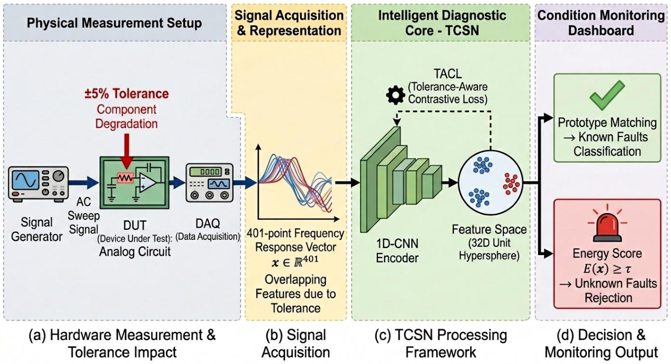
Figure 2.
Sallen-Key second-order Butterworth low-pass filter. Nominal parameters: , , .
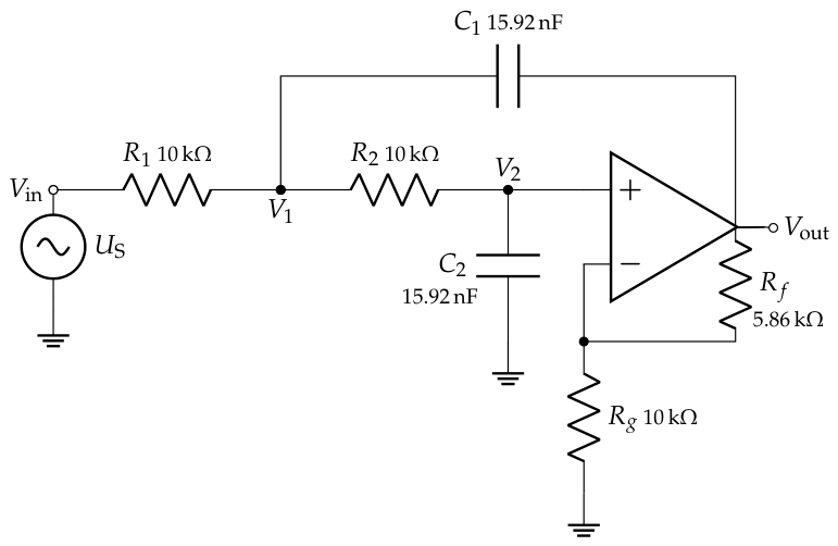
Figure 3.
Simulated Bode plot of the nominal Sallen-Key circuit and residual error relative to the theoretical transfer function (max residual: 0.0012 dB, RMS: 0.0003 dB).
Figure 3.
Simulated Bode plot of the nominal Sallen-Key circuit and residual error relative to the theoretical transfer function (max residual: 0.0012 dB, RMS: 0.0003 dB).
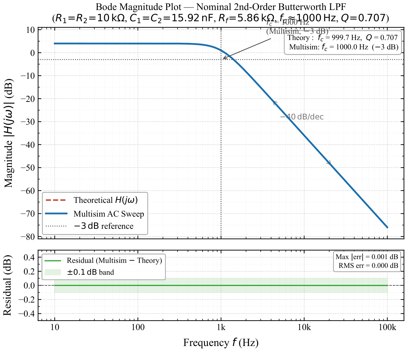
Figure 4.
Voltage gain frequency responses of all ten fault classes of the Sallen-Key circuit. F9 ( open circuit) suffers severe attenuation due to the loss of the forward input signal path. Furthermore, F5 () and F6 () explicitly alter the passband gain in opposite directions owing to their inverse effects on the amplifier gain .
Figure 4.
Voltage gain frequency responses of all ten fault classes of the Sallen-Key circuit. F9 ( open circuit) suffers severe attenuation due to the loss of the forward input signal path. Furthermore, F5 () and F6 () explicitly alter the passband gain in opposite directions owing to their inverse effects on the amplifier gain .
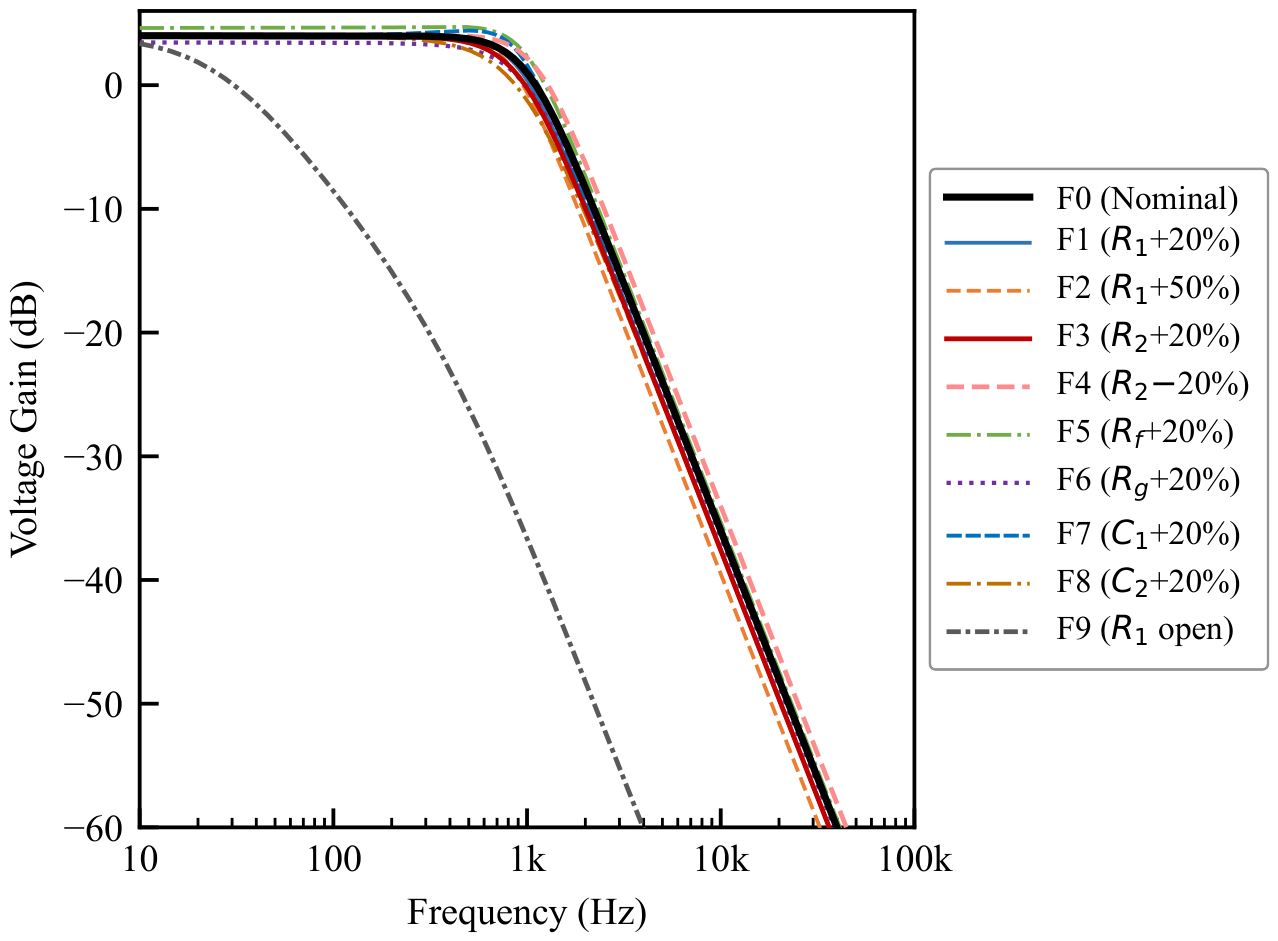
Figure 5.
Pairwise cosine similarity matrix of the nominal frequency-response vectors for all ten fault classes, computed in the original dB-domain. Values close to 1.000 indicate nearly identical responses. F1–F3 and F3–F8 exhibit the highest inter-class similarities (0.999976 and 0.999939, respectively), strongly motivating the design of the fine-grained loss term . F9 ( open circuit) is well-separated from all other classes (similarity 0.922–0.941).
Figure 5.
Pairwise cosine similarity matrix of the nominal frequency-response vectors for all ten fault classes, computed in the original dB-domain. Values close to 1.000 indicate nearly identical responses. F1–F3 and F3–F8 exhibit the highest inter-class similarities (0.999976 and 0.999939, respectively), strongly motivating the design of the fine-grained loss term . F9 ( open circuit) is well-separated from all other classes (similarity 0.922–0.941).
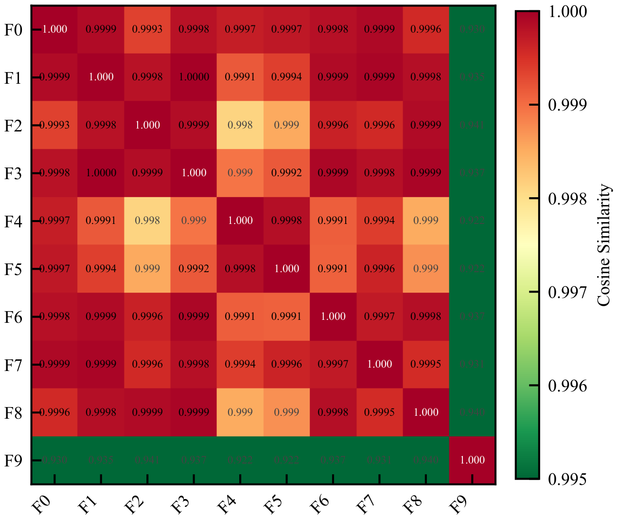
Figure 6.
Monte Carlo tolerance simulation results (N=50 runs, component tolerance ±5%). (a) Frequency-response envelope of the nominal class F0 (5th–95th percentile band), with F1 (+20%) and F9 ( open circuit) overlaid for comparison. (b) Distribution of estimated cutoff frequency under tolerance variation. The F1 fault lies at approximately from the nominal mean, indicating that small parametric deviations are profoundly embedded within the nominal tolerance band and are challenging to isolate using scalar frequency features alone.
Figure 6.
Monte Carlo tolerance simulation results (N=50 runs, component tolerance ±5%). (a) Frequency-response envelope of the nominal class F0 (5th–95th percentile band), with F1 (+20%) and F9 ( open circuit) overlaid for comparison. (b) Distribution of estimated cutoff frequency under tolerance variation. The F1 fault lies at approximately from the nominal mean, indicating that small parametric deviations are profoundly embedded within the nominal tolerance band and are challenging to isolate using scalar frequency features alone.
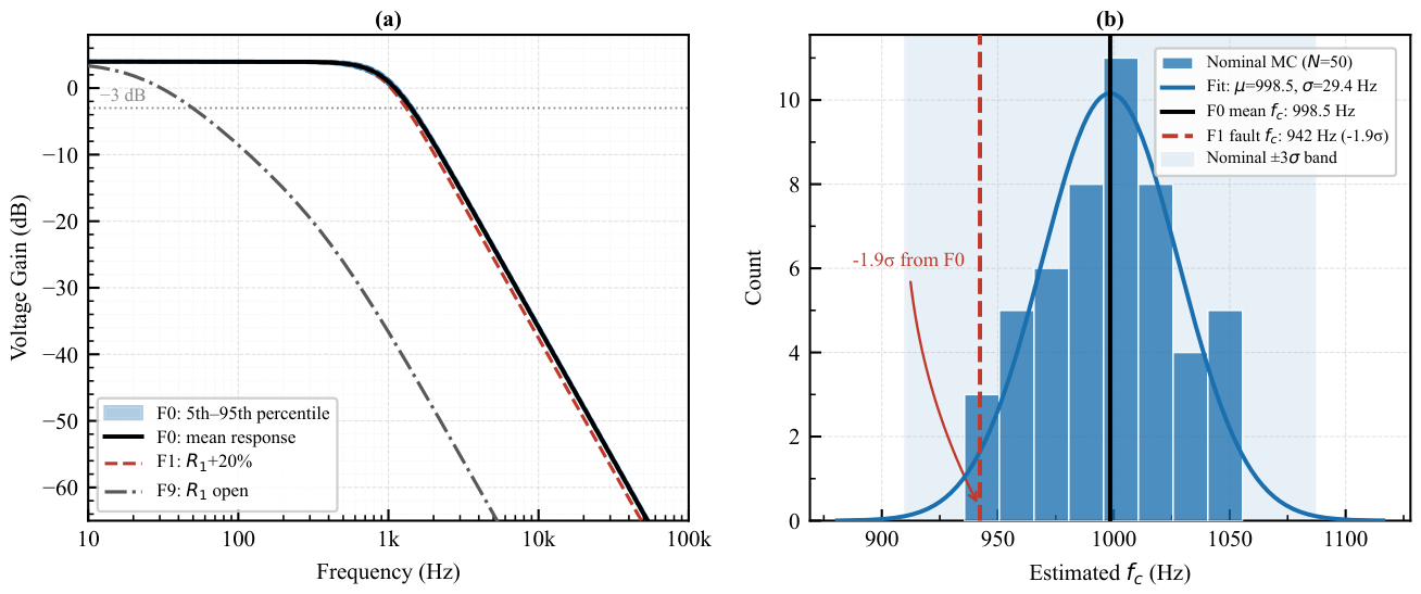
Figure 7.
Detailed processing pipeline of the proposed TCSN framework, comprising three primary stages. (Left) Input representation utilizing z-score normalization on the 401-point input vector. (Middle) The 1D-CNN encoder that progressively extracts robust features from the raw frequency response, mapping it to a 32-dimensional unit-norm embedding . (Right) The Tolerance-Aware Contrastive Loss (TACL) for metric-space calibration during training, and the prototype-based classifier equipped with an energy score detector for open-set inference. Solid arrows denote forward data flow; the dashed arrow denotes backpropagation.
Figure 7.
Detailed processing pipeline of the proposed TCSN framework, comprising three primary stages. (Left) Input representation utilizing z-score normalization on the 401-point input vector. (Middle) The 1D-CNN encoder that progressively extracts robust features from the raw frequency response, mapping it to a 32-dimensional unit-norm embedding . (Right) The Tolerance-Aware Contrastive Loss (TACL) for metric-space calibration during training, and the prototype-based classifier equipped with an energy score detector for open-set inference. Solid arrows denote forward data flow; the dashed arrow denotes backpropagation.
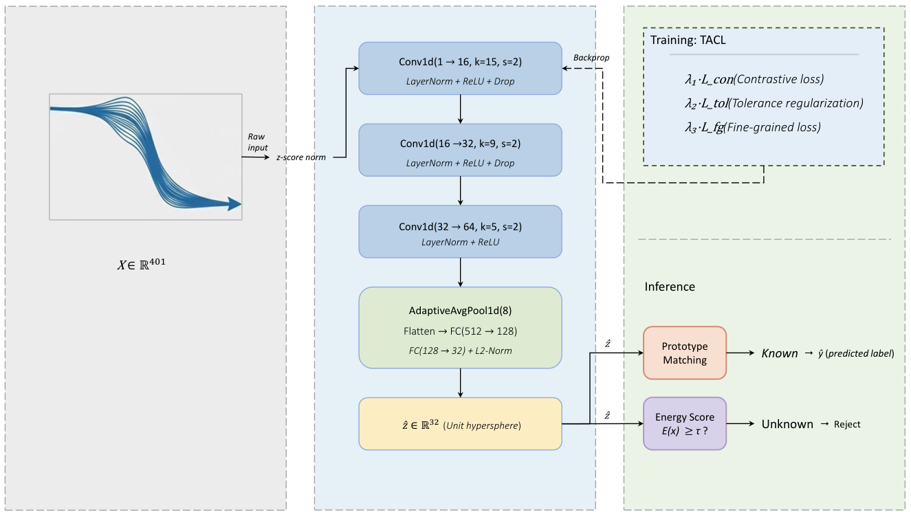
Figure 8.
Evolution of training metrics over 500 epochs. (Left) Total training loss trajectory. (Middle) Evolution of the tolerance compactness loss, highlighting the active optimization of the tolerance term particularly emphasized during Phase 2. (Right) Validation accuracy, demonstrating the effectiveness of the two-phase optimization schedule (Phase 1: epochs 1–200 with only; Phase 2: epochs 201–500 with full TACL), achieving a stable peak accuracy of 94%.
Figure 8.
Evolution of training metrics over 500 epochs. (Left) Total training loss trajectory. (Middle) Evolution of the tolerance compactness loss, highlighting the active optimization of the tolerance term particularly emphasized during Phase 2. (Right) Validation accuracy, demonstrating the effectiveness of the two-phase optimization schedule (Phase 1: epochs 1–200 with only; Phase 2: epochs 201–500 with full TACL), achieving a stable peak accuracy of 94%.
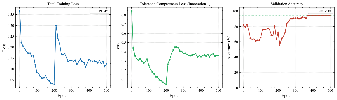
Figure 9.
t-SNE visualization of the latent representations produced by the trained TCSN encoder on the test set. Known fault classes (F0–F9) naturally form compact, topologically separated clusters. In contrast, the OOD unknown samples (U1, U2) occupy interstitial regions structurally distant from the known prototypes, validating the geometric premise of the energy score open-set detector.
Figure 9.
t-SNE visualization of the latent representations produced by the trained TCSN encoder on the test set. Known fault classes (F0–F9) naturally form compact, topologically separated clusters. In contrast, the OOD unknown samples (U1, U2) occupy interstitial regions structurally distant from the known prototypes, validating the geometric premise of the energy score open-set detector.
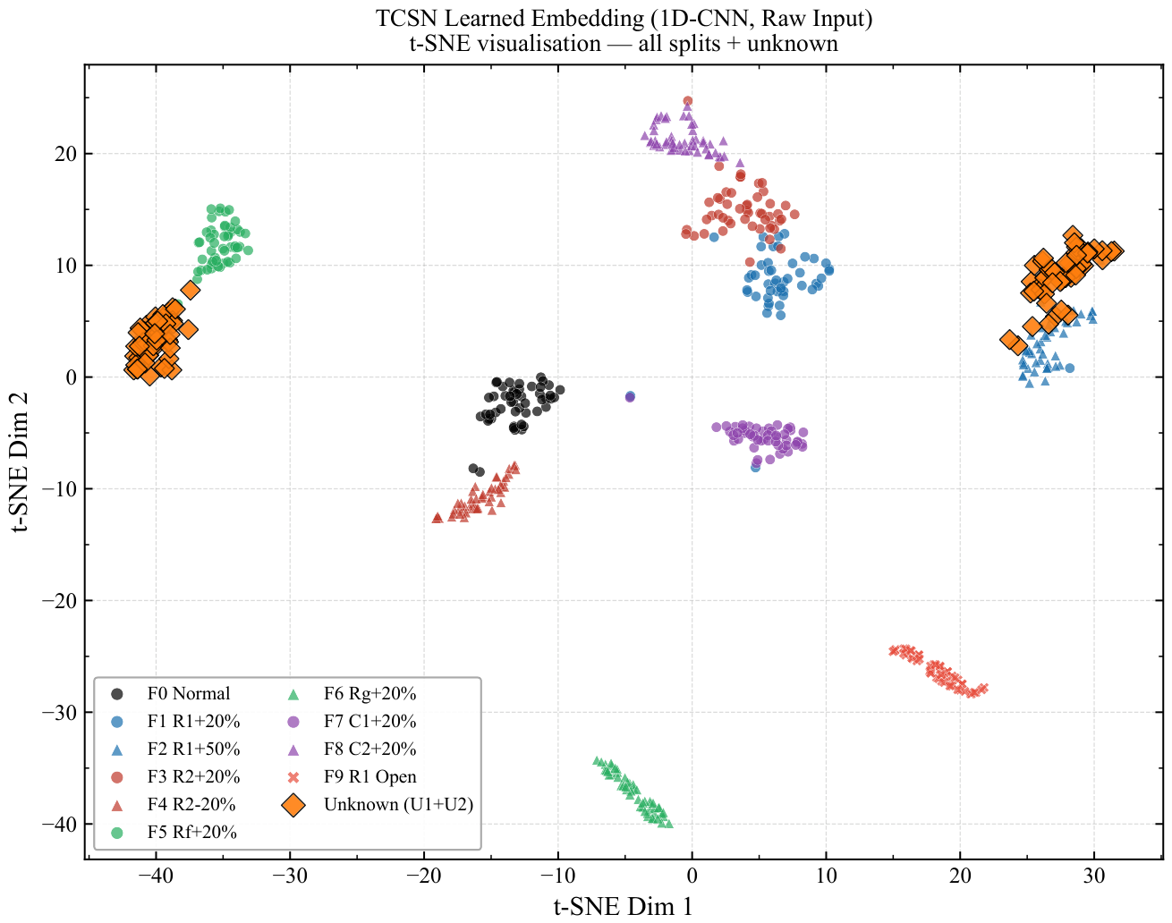
Figure 10.
Confusion matrix detailing the closed-set fault isolation performance (100 test samples, 10 fault classes). Diagonal elements denote correct diagnosis. As theoretically predicted, F3 () exhibits the highest misclassification rate due to its nearly identical frequency response to F1 and F8. Notably, while the proposed method prevents major confusion towards F1, F3 still suffers from a 20% misclassification rate into F8 and receives 10% false positives from F1.
Figure 10.
Confusion matrix detailing the closed-set fault isolation performance (100 test samples, 10 fault classes). Diagonal elements denote correct diagnosis. As theoretically predicted, F3 () exhibits the highest misclassification rate due to its nearly identical frequency response to F1 and F8. Notably, while the proposed method prevents major confusion towards F1, F3 still suffers from a 20% misclassification rate into F8 and receives 10% false positives from F1.
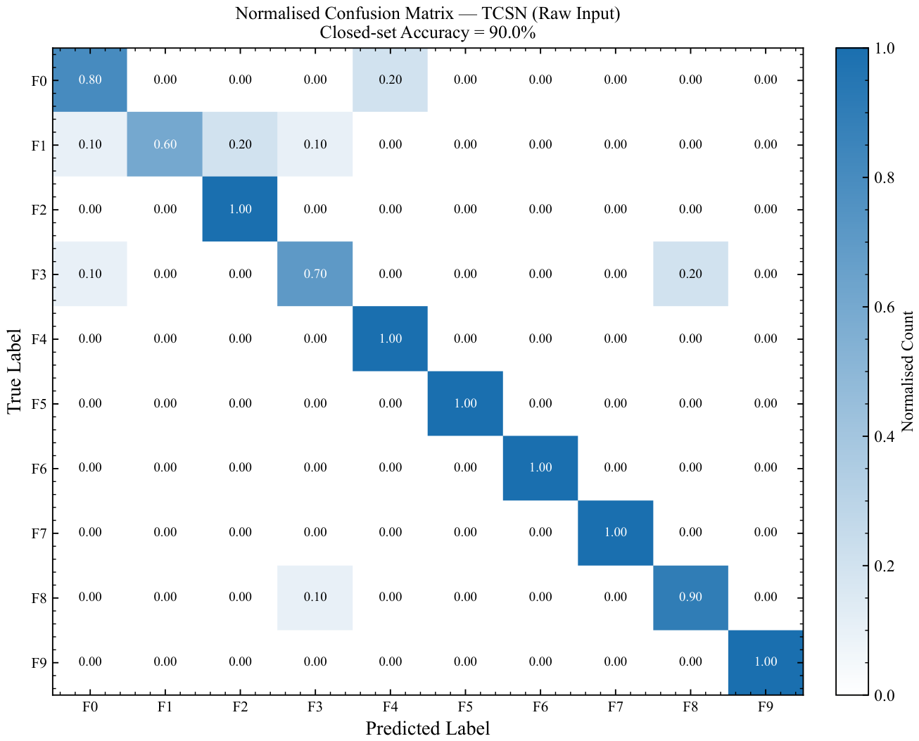
Figure 11.
Evolution of few-shot diagnostic accuracy as a function of the number of support samples per class (n). Results are averaged over five independent trials. TCSN demonstrates a commanding advantage in the extreme few-shot regime (), significantly outperforming all baselines. As n increases beyond 10, data-hungry models (e.g., RF and MLP) gradually surpass TCSN, capitalizing on the abundant labeled data to optimize their larger parameter spaces.
Figure 11.
Evolution of few-shot diagnostic accuracy as a function of the number of support samples per class (n). Results are averaged over five independent trials. TCSN demonstrates a commanding advantage in the extreme few-shot regime (), significantly outperforming all baselines. As n increases beyond 10, data-hungry models (e.g., RF and MLP) gradually surpass TCSN, capitalizing on the abundant labeled data to optimize their larger parameter spaces.
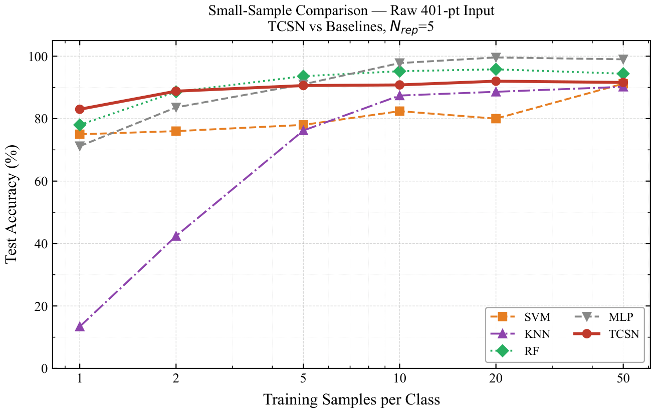
Figure 12.
Receiver Operating Characteristic (ROC) curve for open-set unknown fault detection utilizing the proposed energy score (T=1.0). The high AUROC (0.9309) demonstrates the strong discriminative thresholding capability in separating in-distribution known faults from out-of-distribution unforeseen anomalies.
Figure 12.
Receiver Operating Characteristic (ROC) curve for open-set unknown fault detection utilizing the proposed energy score (T=1.0). The high AUROC (0.9309) demonstrates the strong discriminative thresholding capability in separating in-distribution known faults from out-of-distribution unforeseen anomalies.
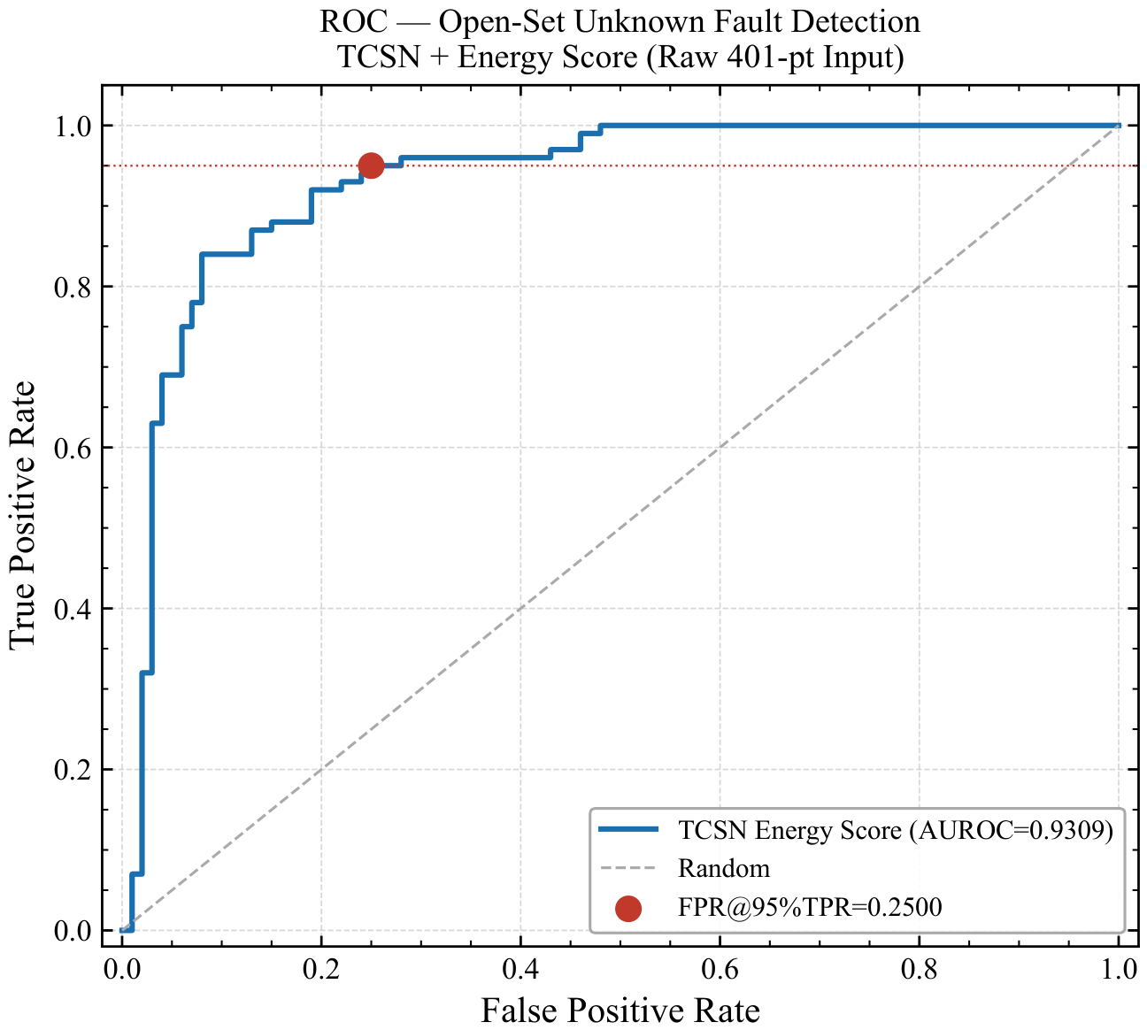
Figure 13.
Frequency histograms detailing the distribution of energy scores for known (F0–F9, blue) and unknown (U1, U2, orange) test samples at T=1.0. Following energy-based theoretical models, known samples map to states of lower energy (mean: , indicating high prototype affinity), whereas unknown samples inherently exhibit higher energy (mean: ), furnishing a statistically robust separation boundary for the threshold .
Figure 13.
Frequency histograms detailing the distribution of energy scores for known (F0–F9, blue) and unknown (U1, U2, orange) test samples at T=1.0. Following energy-based theoretical models, known samples map to states of lower energy (mean: , indicating high prototype affinity), whereas unknown samples inherently exhibit higher energy (mean: ), furnishing a statistically robust separation boundary for the threshold .
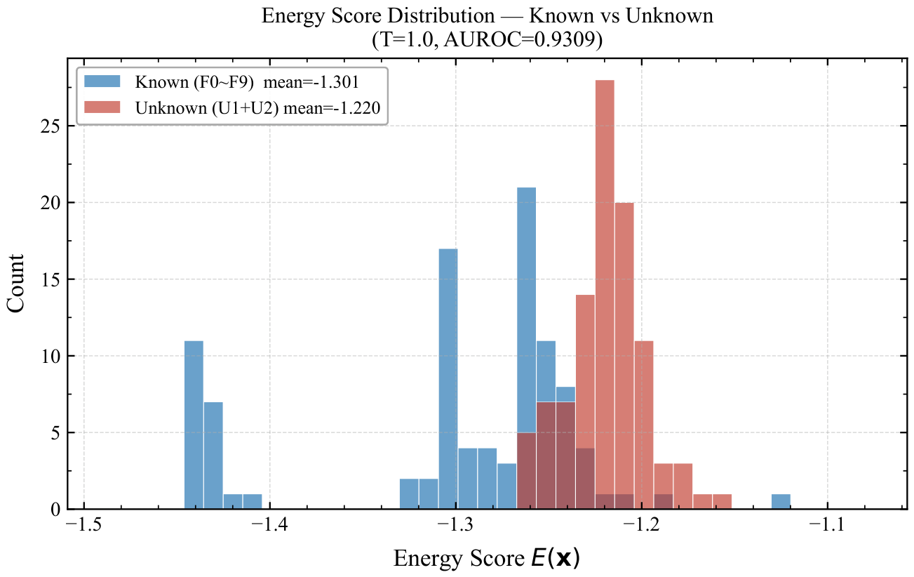
Figure 14.
Model robustness under additive white Gaussian noise (AWGN). (a) Closed-set accuracy trajectories vs. SNR. Standard classifiers (MLP, SVM, KNN) suffer catastrophic collapse at 30 dB. RF shows excellent resilience at mild/moderate noise levels (30 dB, 20 dB) due to ensemble voting, but collapses at extreme noise (10 dB). TCSN demonstrates the most graceful degradation, ultimately outperforming all baselines at the most severe 10 dB level. (b) Open-set AUROC of TCSN vs. SNR, exhibiting a non-monotonic trend due to extreme noise-induced topological embedding drift.
Figure 14.
Model robustness under additive white Gaussian noise (AWGN). (a) Closed-set accuracy trajectories vs. SNR. Standard classifiers (MLP, SVM, KNN) suffer catastrophic collapse at 30 dB. RF shows excellent resilience at mild/moderate noise levels (30 dB, 20 dB) due to ensemble voting, but collapses at extreme noise (10 dB). TCSN demonstrates the most graceful degradation, ultimately outperforming all baselines at the most severe 10 dB level. (b) Open-set AUROC of TCSN vs. SNR, exhibiting a non-monotonic trend due to extreme noise-induced topological embedding drift.
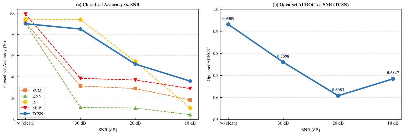
Figure 15.
Performance profiling across ablation variants. Note that the FPR metric is plotted as FPR@95%TPR to ensure a consistent “higher-is-better” visual representation. The Full TCSN (blue) achieves the optimal equilibrium. Removing devastates open-set detection (AUROC drop: 0.3793). Removing severely harms fine-grained closed-set accuracy (: %). Replacing the energy score strictly penalizes OOD separability without affecting closed-set metrics.
Figure 15.
Performance profiling across ablation variants. Note that the FPR metric is plotted as FPR@95%TPR to ensure a consistent “higher-is-better” visual representation. The Full TCSN (blue) achieves the optimal equilibrium. Removing devastates open-set detection (AUROC drop: 0.3793). Removing severely harms fine-grained closed-set accuracy (: %). Replacing the energy score strictly penalizes OOD separability without affecting closed-set metrics.
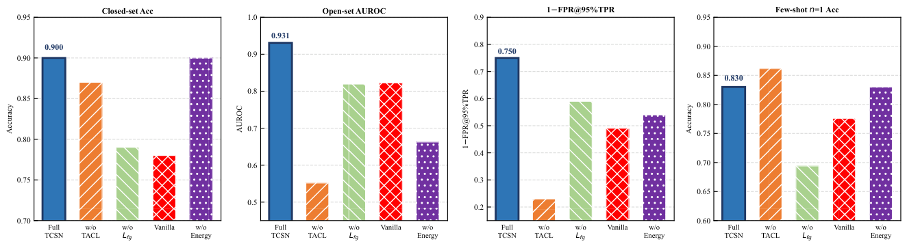

Table 1.
Nominal Component Values and Filter Parameters.
| Parameter | Value | Parameter | Value |
|---|---|---|---|
| Q | |||
| K | |||
| Sim. residual |
Table 2.
Fault Class Catalog.
| ID | Component | Deviation | Split |
|---|---|---|---|
| F0 | — | Nominal | Train/Val/Test |
| F1 | Train/Val/Test | ||
| F2 | Train/Val/Test | ||
| F3 | Train/Val/Test | ||
| F4 | Train/Val/Test | ||
| F5 | Train/Val/Test | ||
| F6 | Train/Val/Test | ||
| F7 | Train/Val/Test | ||
| F8 | Train/Val/Test | ||
| F9 | Open () | Train/Val/Test | |
| U1 | (compound) | Open-set only | |
| U2 | Open-set only |
Table 3.
Dataset Split Configuration.
| Split | Classes | Samples/class | Total | Purpose |
|---|---|---|---|---|
| Train | F0–F9 (10) | 30 | 300 | Metric learning |
| Val | F0–F9 (10) | 10 | 100 | Hyperparameter selection |
| Test | F0–F9 (10) | 10 | 100 | Closed-set evaluation |
| Unknown | U1, U2 (2) | 50 | 100 | Open-set evaluation |
| Total | 1,100 | (Unknown excluded from training) | ||
Table 4.
Encoder Architecture.
| Layer | Output Shape | Normalization |
|---|---|---|
| Conv1d (1→16, k=15, s=2) | LayerNorm + ReLU | |
| Conv1d (16→32, k=9, s=2) | LayerNorm + ReLU | |
| Conv1d (32→64, k=5, s=2) | LayerNorm + ReLU | |
| AdaptiveAvgPool1d (8) | — | |
| Flatten | — | |
| FC (512→128) | LayerNorm + ReLU | |
| FC (128→32) + L2-Norm | L2 normalization |
Table 5.
Per-Class F1-Scores for Closed-Set Fault Diagnosis on the Test Set.
| Fault Class | F1 Score |
|---|---|
| F0 (Nominal) | 0.80 |
| F1 () | 0.82 |
| F2 () | 0.87 |
| F3 () | 0.62 |
| F4 () | 0.91 |
| F5 () | 0.95 |
| F6 () | 1.00 |
| F7 () | 1.00 |
| F8 () | 0.86 |
| F9 ( open circuit) | 1.00 |
| Macro-F1 | 0.88 |
| Weighted-F1 | 0.88 |
Table 6.
Closed-Set Test Accuracy Under Full-Data Regime.
| SVM | KNN | RF | MLP | TCSN (ours) | |
|---|---|---|---|---|---|
| Accuracy | 91.2% | 90.2% | 94.4% | 99.0% | 90.0% |
Table 7.
Few-Shot Diagnostic Accuracy (%) vs. Number of Support Samples per Class.
| n/class | SVM | KNN | RF | MLP | TCSN (ours) |
|---|---|---|---|---|---|
| 1 | 75.0 | 13.4 | 78.0 | 71.2 | 83.0 |
| 2 | 76.0 | 42.4 | 88.6 | 83.6 | 90.4 |
| 5 | 78.0 | 76.2 | 93.6 | 91.0 | 92.4 |
| 10 | 82.4 | 87.4 | 95.2 | 97.8 | 92.8 |
| 20 | 80.0 | 88.6 | 95.8 | 99.6 | 94.2 |
| 50 | 91.2 | 90.2 | 94.4 | 99.0 | 95.4 |
Table 8.
Open-Set Detection Performance vs. Temperature Scale (T).
| Method / T | AUROC | FPR@95%TPR | Note |
|---|---|---|---|
| TCSN, | — | — | Degenerate |
| TCSN, | — | — | Suboptimal |
| TCSN, | 0.9309 | 0.2500 | Optimal |
| Known energy: | |||
| Unknown energy: | |||
Table 9.
Robustness to AWGN Noise (Closed-Set Accuracy / Open-Set AUROC).
| SNR | SVM | KNN | RF | MLP | TCSN (ours) |
|---|---|---|---|---|---|
| ∞ (clean) | 91.2% | 90.2% | 94.4% | 99.0% | 90.0% / 0.9309 |
| 30 dB | 31.4% | 11.2% | 93.8% | 38.6% | 85.0% / 0.7598 |
| 20 dB | 29.0% | 10.6% | 54.4% | 37.0% | 52.0% / 0.6083 |
| 10 dB | 18.2% | 4.4% | 10.6% | 29.0% | 36.0% / 0.6847 |
Table 10.
Ablation Study Results.
| Variant | Acc. | AUROC | FPR@95% | ||
|---|---|---|---|---|---|
| Full TCSN | 90% | 0.9309 | 0.2500 | 0.830 | 0.906 |
| w/o TACL | 87% | 0.5516 | 0.7700 | 0.862 | 0.868 |
| w/o | 79% | 0.8193 | 0.4100 | 0.694 | 0.670 |
| Vanilla | 78% | 0.8226 | 0.5100 | 0.776 | 0.758 |
| w/o Energy | 90% | 0.6626 | 0.4600 | 0.830 | 0.906 |
Acc.: Closed-set test accuracy. : Few-shot support set accuracy. w/oTACL: Replaces with standard contrastive loss. w/o: Removes the fine-grained hard-pair term. Vanilla: Removes both and . w/oEnergy: Replaces energy score with min-distance threshold.
Disclaimer/Publisher’s Note: The statements, opinions and data contained in all publications are solely those of the individual author(s) and contributor(s) and not of MDPI and/or the editor(s). MDPI and/or the editor(s) disclaim responsibility for any injury to people or property resulting from any ideas, methods, instructions or products referred to in the content. |
© 2026 by the authors. Licensee MDPI, Basel, Switzerland. This article is an open access article distributed under the terms and conditions of the Creative Commons Attribution (CC BY) license (http://creativecommons.org/licenses/by/4.0/).
Copyright: This open access article is published under a Creative Commons CC BY 4.0 license, which permit the free download, distribution, and reuse, provided that the author and preprint are cited in any reuse.