

Submitted:
01 July 2026
Posted:
02 July 2026
You are already at the latest version
Abstract
This study demonstrates the successful application of passive seismic interferometry, specifically through the autocorrelation function, to extract high-resolution P-wave reflections from seismic data acquired during hydraulic fracturing. This application demonstrates the efficacy of extracting high-resolution P-wave reflectivity using hydraulic fracturing-induced seismic noise, a previously underexplored source for exploration-scale imaging. Stacking these reflections allows the construction of seismic sections at zero offsets. Typically, this technique uses data based on environmental noise and earthquakes. However, this study used measurements obtained during hydraulic fracturing in the Potiguar Basin of Northeast Brazil. We applied a processing sequence that included the Gaussian Smoother Filter to generate a smoothed amplitude spectrum and to extract the best body-wave component of Green’s function. We whitened the spectrum to remove any unwanted effects from the sources. The resulting seismic sections were compared with seismic lines acquired near the study area and interpreted in light of the available geological information. The seismic images were constructed in 2D and projected into 3D, with reflectors exhibiting high resolution and lateral continuity. Deeper reflectors align well with available geological and geophysical data; however, validation of the shallowest boundaries remains limited by the absence of high-resolution reference data in this area. The estimated time depth reached 2s. Validation of the shallowest reflectors (< 500 m depth, corresponding to the Cenozoic cover and upper Jandaíra Formation) is limited by the absence of high-resolution geological data at the survey site. No shallow boreholes or outcrop transects are available to confirm the depth and continuity of these interfaces. Legacy active seismic lacks resolution above ≈300 m depth. Consequently, our interpretation of shallow reflectors relies on regional geological maps and extrapolation from nearby wells, introducing uncertainty. Future work should include shallow drilling or high-resolution GPR surveys to validate the uppermost 500 m of the autocorrelation sections. Additionally, the maximum penetration depth of the S-wave velocity model (approximately 180 m) is constrained by the short maximum offset (1,450 m), precluding integration with deeper autocorrelation-derived reflectivity. We calculated cross-correlations using two configurations—one with the longest available offset (1,450 m) and one within a single line—to obtain S-wave velocity models and determine the maximum penetration depth (approximately 180 m) achievable with the current acquisition geometry.
Keywords:
passive seismic interferometry
; autocorrelation function
; high-resolution passive seismic
; potiguar basin
1. Introduction
The term ”interferometry” refers to the study of interference phenomena between pairs of signals to acquire information from their differences and similarities [1,2]. According to the definition above, in ambient seismic noise interferometry (ANSI), the empirical Green’s function (EGF)cross-correlation between two receivers can be retrieved: one receiver acts as a virtual source and the other as a receiver. In practice, this method requires computing cross-correlations and subsequently stacking the resulting waveforms [1,3,4]. Over the past two decades, seismic interferometry has established itself as a method applicable in various areas of geophysics [5,6,7,8]. In single-station applications, computing the autocorrelation function (ACF) of continuous passive records yields an empirical trace that directly represents the zero-offset reflection response beneath a receiver. Stacking each station’s autocorrelogram provides a proxy image of the subsurface [9]. Seismic interferometry (SI) is a well-established method for imaging subsurface structures [10,11,12]. Typically, ambient noise is used as input data in the autocorrelation function to determine crustal structures and Moho reflections [9,13]. Cross-correlation has also been widely applied to extract valuable information in the study of the Earth’s crust [14]. Its application at exploration scales has increased recently, particularly at local scales, where the properties of surface waves can be used to obtain velocity models and S-wave tomography [15,16,17], as well as high-resolution seismic imaging from ACF at the exploration scale [18]. In this context, passive seismic interferometry can be used for geophysical exploration and other applications such as engineering. Many studies have used cross-correlations to estimate S-wave velocity model parameters. Recent studies have examined applications in mapping important exploration areas in mining [16,19] and advanced monitoring of tailings dams [20]. It also has applications in the oil and gas industries, typically as a complement to active seismic events [21]. Additionally, it has been used in geotechnical applications integrated with surface methods, such as MASW [22] and a variation of the seismic interferometry method [15]. Although seismic interferometry using autocorrelation functions has been applied to deep investigations, these studies typically employed a limited frequency range. Consequently, there remains a notable gap in leveraging autocorrelation functions at frequencies exceeding 20 Hz for high-resolution P-wave reflectivity imaging at exploration scales. This study addresses this gap by demonstrating the efficacy of hydraulic fracturing-induced seismic noise—a previously underexplored transient source—for generating reflectivity images with approximately 20 m vertical resolution. For deep objectives, such as Moho reflectivity and crustal structure, a low-frequency range is used [13,23,24,25]. However, investigations at smaller scales, such as geothermal system exploration [26], sedimentary basin exploration [27,28], and mining applications [18] require a relatively high-frequency range. This study adapts established autocorrelation-based seismic interferometry workflows (e.g., Bensen et al. 2007) by optimizing Gaussian smoothing parameters and bandpass filters to extract P-wave reflectivity at frequencies up to 30 Hz from hydraulic fracturing-induced noise—a source not previously applied for this purpose at exploration scales. Our novelty lies in demonstrating the efficacy of this approach using seismic data acquired during hydraulic fracturing, a previously underexplored noise source for generating high-frequency reflectivity images that delineate subsurface lithological characteristics. The data used were acquired by monitoring a hydraulic fracturing treatment conducted in the Potiguar Basin, NE Brazil, as shown in Figure 1A. Our results demonstrate that the calculated autocorrelation functions enable the extraction of reflected P-waves across a wide frequency range (up to 30 Hz), yielding seismic sections with significantly higher resolution (for example, resolving features near 20 m) than that typically achieved with ambient noise interferometry, which is crucial for detailed exploration. We evaluated these results using the available geological and geophysical information, which validated the shallow lithologies of the northern zone of the Potiguar Basin. This approach provides high-resolution reflectors associated with the three main lithological bodies of the area: the Jandaira Formation, the Açu Formation, and the top of the basement. In contrast, we estimated the maximum possible cross-correlation calculations and S-wave velocity models for the same data. A secondary objective is to determine whether the available acquisition geometry permits integration of autocorrelation-derived reflectivity profiles with cross-correlation-derived S-wave velocity models. Specifically, we test whether the maximum offset (1,450 m) provides sufficient wavelength penetration to generate velocity models that overlap in depth with the autocorrelation reflectivity sections.
2. Survey Area and Data
Noise records were obtained near two wells in the northern part of the Potiguar Basin, specifically in the Canto do Amaro field in Northeast Brazil (Figure 1).
Fifteen gigabytes of data were recorded from 182 seismic vertical sensors (Sercel L4-A geophones) with a natural frequency of 2 Hz, as depicted in Figure 1 and Table 1. These sensors used a RefTek 125-A acquisition system (Texan). The data were recorded continuously at a sampling frequency of 200 Hz for ten hours. The raw noise data from this monitoring experiment are presented in Figure S1.1 of the Supplementary Material.
Well-defined linear receiver lines characterize the acquisition geometry of the data. Although this deployment was not originally optimized for passive interferometry—resulting in limited azimuthal coverage and sparse lateral sampling in some areas—the geographic intersection of lines 1, 2, and 3 enabled cross-validation of zero-offset reflection profiles directly over the source zone. Future deployments should incorporate denser 2D or 3D arrays to improve lateral resolution and reduce spatial aliasing. This intersection is located approximately above the point where fracturing was performed and enables the evaluation and comparison of the results for each corresponding seismic section. Furthermore, the linear arrangement of all receivers allows for a higher lateral resolution. The data were continuously recorded for five hours each day for two days. The recordings included both ambient noise and noise induced by hydraulic fracturing. These data were used in previous studies by [29] and [30], and their results served as the basis for the present study.
3. Geological Setting
The Potiguar Basin is located at the extreme northeastern tip of Brazil on the equatorial margin of South America (Figure 1A). It is positioned at the intersection of the eastern and equatorial Atlantic margins, representing a key tectonic feature formed during the Mesozoic breakup of Pangaea and the subsequent separation of the South American and African plates [31,32]. The basin encompasses both onshore and offshore domains, covering an area of approximately 48,000 km2, and its origin is linked to dextral transform shearing along the equatorial margin [32,33]. The study area is situated in the northern onshore sector of the basin, specifically within the Canto do Amaro oil field, where a relatively simple and undeformed shallow stratigraphic framework prevails (Figure 1B). The tectono-sedimentary evolution of the Potiguar Basin comprises three major depositional sequences: rift, transitional, and post-rift (drift) phases [34,35]. The rift sequence, which is deeply buried in the central grabens and does not crop out in the study area, developed during the Neocomian to Early Barremian under a predominantly extensional-to-transtensional regime [31,36]. This was followed by an Aptian transitional marine sequence, which marked the first marine incursion. Finally, the post-rift sequence was deposited from the Albian to the Campanian, characterized by broad thermal subsidence that covered the entire basin and extended beyond the rift boundaries [34,35]. The subsurface and outcropping geology in the northern onshore sector of the basin is dominated by post-rift successions, specifically the Açu and Jandaíra formations, which are capped by younger Cenozoic deposits (Figure 1B). The Açu Formation, of Albian to Cenomanian age, primarily consists of siliciclastic rocks deposited in fluvial to shallow marine environments. The lower section of this formation is composed of thick reddish conglomerates and sandstones with thin intercalations of shales and siltstones, whereas the upper section comprises sandstones interbedded with greenish shales [36,37]. This formation constitutes the primary oil reservoir in the Canto do Amaro field and is the main target of the hydraulic fracturing operations monitored in this study [30]. Overlying the Açu Formation with a gradational contact is the Jandaíra Formation, a widespread carbonate platform of Turonian to Campanian age [34,38,39]. This unit consists of marine-derived carbonates, mainly calcilutites and calcarenites, deposited in tidal and shallow shelf environments [35,37]. In the study area, the Jandaíra Formation is exposed at the surface as limestone (Figure 1B) and constitutes the uppermost continuous lithological layer before the unconsolidated Cenozoic cover, which includes the siliciclastic Barreiras Formation and recent alluvial sediments [30]. From a structural and geophysical perspective, the geological characteristics of the northern Potiguar Basin provide a highly favorable setting for passive seismic interferometry. The post-rift strata in this region, including the Açu and Jandaíra formations, exhibit sub-horizontal dips and remarkable lateral continuity [40]. Consequently, the subsurface can be accurately modeled as a sequence of homogeneous, well-defined lithological layers, specifically the Cenozoic cover, Jandaíra carbonates, Açu siliciclastics, and the underlying crystalline basement. The lack of significant lateral velocity variations and the absence of complex structural deformation in the shallow subsurface enhance the reliability of the zero-offset reflections retrieved from autocorrelation functions.
4. Methodology
In this study, we used two methodologies to calculate the autocorrelation function (ACF) and retrieve the S-wave velocity from the cross-correlations between seismic stations. The background seismic noise characterization for this asset was previously established by [30], and the main features were considered for the frequency analysis. The amplitude spectrum of the entire record for the first station in Lines 02 and 04 is presented in Figure S1.2 of the Supplementary Material. The spectrum shows intervals of mini-fracturing and fracturing processes and several discrete resonant frequencies that contribute to the total power spectral density.
4.1. Auto-Correlation Function
While continuous recording spanned 5 h each day, the actual hydraulic fracturing treatment occurred exclusively during the final hour of acquisition. We isolated this specific high-energy window for autocorrelation analysis. Preprocessing began by slicing the raw records into one-hour blocks, followed by mean and trend removal and a 10% cosine taper. A Fourier transform was then applied, as depicted in the workflow diagram in Figure 2.
We calculated the amplitude spectrum and applied a smoothing Gaussian filter. We obtained a whitened spectrum by dividing the raw spectrum by the smoothed spectrum [13,18,41]. The Gaussian smoothing filtering process and spectral whitening are shown in Figure S2 of the Supplementary Material. The whitening process is essential for reducing the effects of microseismic peaks because it controls the correlation results. After the whitening process, it was necessary to reduce the frequency range to the desired spectrum, which was achieved by applying a zero-phase band-pass filter. We tested multiple high-frequency cutoffs, specifically 16, 20, and 30 Hz, to evaluate the impact of higher frequencies on image resolution. Because the local stratigraphic boundaries are well established from legacy geological data, varying these bandpass filters allowed us to pinpoint the exact frequency range required to clearly resolve the known lithological contacts. Higher frequencies were required to achieve the necessary resolution to discriminate lithologic layers in the study area. Applying a Gaussian filter aims to achieve a broader filter response and smoother filtering. For this purpose, larger standard deviations were used, and the smoothing bandwidth was set to 15 Hz. We also evaluated a 1-bit filter, which is widely used in the processing flow for surface wave retrieval and in the processing of the auto-correlation function [13,15,16,19]). However, the 1-bit filter yielded results of varying quality, likely due to its strong nonlinearity, which can distort amplitude information crucial for reflectivity studies, and ultimately required an AGC filter for amplitude balancing. In contrast, the Gaussian smoothing filter provided superior results, effectively smoothing the spectrum while better preserving the relative amplitudes that are essential for accurate P-wave reflectivity imaging. Another important factor in the processing sequence is the size of the correlation window [41]. We started with a window of 60 s and then reduced it to 30 and 15 s. The 15-s window provided the best results. Autocorrelation wiggles for different frequency ranges are presented in Figure S4 of the Supplementary Material, which shows the autocorrelation functions calculated for all stations of Line 02. The figure illustrates the continuity of the amplitudes at different depths, the effect of frequency cuts in each section, and the changes in the definition of each reflector after the seismic image is completed (Figure 4). Applying an inverse Fast Fourier Transform (IFFT) converts the conditioned spectra back to the time domain, yielding individual station autocorrelation traces. As a final calculation step, we linearly stacked all the windows obtained from the autocorrelation process.
4.2. Passive Seismic Interferometry
Given the current acquisition geometry, the objective of cross-correlation-based wave-velocity extraction was to determine the maximum possible penetration depth for a 1D S-wave velocity model. We considered two configuration options for the procedure. First, all stations on Line 3 were used as receptors, with the easternmost station on line 4 as the virtual source. This was done to use the largest offset available to extract the longest wavelength possible. Second, only line 03 was used, with the easternmost station near the well as the virtual source and the remaining stations as the receptors. The workflow used is shown in Figure 3 and is based on [41]. The raw data were evaluated to determine the optimal S-wave retrieval lengths. For this purpose, the cross-correlation was evaluated with lengths of 1, 2, 3, and 5 h. The results are presented in Figure S4 of the Supplementary Material, indicating that 1 h is sufficient to robustly extract surface waves.
We executed the standard processing workflow through six consecutive stages: 1) conducting frequency analysis to determine the optimal retrieval window; 2) applying a linear detrending operator; 3) implementing a zero-phase bandpass filter based on the spectrum; 4) normalizing the datasets using 1-bit temporal and spectral whitening; and 5) computing classical cross-correlations followed by phase-weighted stacking (PWS) [42]. This choice, consistent with the findings of [30] and confirmed in our study, effectively enhances coherent signals while suppressing the incoherent noise inherent to our dataset. 6) Dispersion curve inversions were performed to resolve the local shear-wave velocity profile. Conventionally, linear stacking combines processed cross-correlation data windows directly over given time intervals. This basic approach often struggles in a complex noise environment, where sources are not isotropically distributed across the oil field. Phase-weighted stacking (PWS) addresses this issue by using phase coherence to weight the data. Instead of relying strictly on standard amplitude sums, the algorithm uses phase consistency to downweight inconsistent portions of the linear stack. This specific mechanism targets the incoherent noise inherent in the records while actively enhancing the underlying coherent wavefield. In our cross-correlation analysis, the performance gap between the two methods was evident. Linear stacking retains a higher degree of incoherent noise, which can obscure weaker features, whereas PWS provides a significantly improved signal-to-noise ratio. This phase-based enhancement suppresses background noise artifacts, enabling the easier and cleaner identification of the retrieved Rayleigh waves along the channels. The selection of a phase-weighted scheme over a standard linear stack directly aligns with the effective processing strategies established by Silva et al. (2021) for this acquisition geometry.
The processing flow for this project was implemented using ObsPy [43], a software that allows data plotting and the application of several seismological processing algorithms. The dispersion curve and inversion process were determined using Geopsy [44], an open-source software package for conducting geophysical experiments. Among its capabilities is the application of the Multichannel Analysis of Surface Waves (MASW) method [45] for dispersion curve calculation, as well as the Dinver inversion module, which uses the neighborhood algorithm for velocity curve inversion. The frequency range used to calculate the dispersion curves was 2-16 Hz. Within this range, there was constant noise with a relatively constant amplitude, as shown in the frequency spectrum in Supplementary Figure S2. We selected the lowest available frequency window (2–16 Hz) and leveraged the maximum source-receiver offsets to capture the longest possible surface wavelengths, thereby maximizing structural depth penetration during inversion. The S-wave velocity model results were validated by comparing them with the ground roll values commonly used in the area. In contrast, the P-wave velocity was validated using the information published by [46]. These values were obtained from seismic acquisitions in the same area and validated using consolidated geological information.
5. Results and Interpretations
5.1. Seismic Section, and Auto-Correlation Functions
We calculated the autocorrelations for the final hour of acquisition, during which hydraulic fracturing occurred. After processing the data according to the scheme shown in Figure 2, each station was plotted to create the corresponding seismic sections. The results obtained for Line 03 are shown in Figure 4 for the three frequency ranges of 2-16, 2-20, and 2-30 Hz. Each seismic line in the figure clearly identifies several reflectors and their positions. It is important to note that the applied processing prioritizes the extraction of the low-frequency body waves. The resulting processing pipeline achieved a coherent imaging depth corresponding to a two-way travel time of 2 s.
We obtained equally consistent and well-defined reflectors along the remaining lines, with reflectors at similar depths and very consistent lithology. Figure 5 and Figure 6 show the results for Lines 01 and 02, respectively. We observed an improvement in resolution with the application of a broader frequency range. Each reflector improves its definition and maintains continuity, even at frequencies of up to 30 Hz. One plausible reason for the obtained resolution is the acquisition geometry at the hydraulic fracturing point. A detailed comparison between ambient noise and fracturing intervals is shown in Supplementary Figure S6 of the Supplementary Material, which compares an hour of processed data obtained only when ambient noise prevails with the result of processing during the interval when fracturing occurred. Visual comparison suggests that records captured during active fluid injection yield higher-quality imaging than those from background ambient noise alone, as evidenced by improved reflector continuity and definition in Supplementary Figure S6. However, quantitative signal-to-noise ratio analysis was not performed to confirm this observation. Background noise alone successfully maps the primary structural horizons, as shown in Supplementary Figure S6, but completely misses the weaker or deeper interfaces. This resolution gap becomes even more pronounced as the bandpass filter is widened to include higher frequencies.
In contrast, Figure 7(i) shows an active-source seismic line acquired near the study area. It is evident that the shallow zone near the surface was not resolved. However, good resolution was observed at depth, showing parallel and continuous reflectors.
Considering the geological context, the primary reflectors obtained through autocorrelation data reflect subsurface geometry. As shown in Figure 7(h), reflectors AP and CP correspond closely in two-way travel time with those obtained from legacy active data, which are referred to as reflectors AA and BA, respectively ( Figure 7(j)). Based on two-way travel time alignment with legacy seismic data and regional geological context, we tentatively interpret reflectors AP and CP as the top of the Jandaira Formation and basement, respectively. Reflector BP likely corresponds to the top of the Açu Formation, though this assignment remains interpretive given the limited direct validation data at this depth (Figure 7(h)). Additionally, the reflector DP, located at a greater depth, lacks information for comparison. To illustrate the consistency of the results and form an interpretable high-resolution seismic model, a 3D representation of the three seismic sections is shown in Figure S7 of the Supplementary Material for each frequency cutoff used in the study: 2-16 Hz, 2-20 Hz, and 2-30 Hz. The consistency and continuity of each reflector can be observed at the intersection point of the three seismic sections, even in the highest frequency range.
5.2. S-Wave Velocity Model and Crosscorrelation Functions
We obtained another key result: the cross-correlations between stations determined the surface wave velocity. This calculation aimed to determine the maximum penetration achievable using the current acquisition geometry.
We evaluated two separate cross-correlation configurations. The first involved using the largest offset among all acquisition geometries. In this configuration, the receiver located furthest east on Line 04 was used as the virtual source, and all stations on Line 03 were used as receivers ( Figure 1B). The largest and shortest offsets were 1450 m and 750 m, respectively. This cross-correlation configuration will be referred to as "Cross01".
A seismogram of the surface wave retrieval is shown in Figure S8.1 of the Supplementary Material. A frequency range of 2-16 Hz was used for this calculation. We chose the lowest frequency range to maximize penetration, and given the relative geological homogeneity of the study area, a higher-resolution capacity was not necessary. The result had a lower signal-to-noise ratio and greater interference, mainly towards the end of the line. However, the wave train could be extracted completely for this offset. The other configuration considered only line 3 for the cross-correlation calculations. The station furthest to the east, near the well, served as the virtual source, and the remaining stations served as receivers. The offset between the virtual source and the first receiver was 10 m, and the last receiver was located 660 m from the virtual source. This cross-correlation is referred to as Cross02 in this study. A frequency cutoff of 2–16 Hz. The resulting seismogram with the extracted surface waves is shown in Figure S8.2 of the Supplementary Material and displays a good signal-to-noise ratio. Notably, the surface wave train could not be extracted in the first 200 m of the line, where the start of each trace was not observable. Figures S9.1 and S9.2 show the results of the dispersion curves and velocity models obtained for the two studied cases, Cross01 and Cross02, respectively. The S-wave velocities in both cases were similar to the commonly reported ground roll values in the area, approximately 1,350 m/s. In addition, the weathered layer was approximately 50 m thick. We estimated a maximum penetration depth of approximately 180m, with a wavelength of approximately 540 m. The short distance of 10 m between the virtual source and the first receiver in Cross02, relative to the wavelength of 540 m, explains why it was not possible to obtain complete traces along the first 200 m of the Cross02 seismogram. In our case, the offset between the virtual source and the first receiver should have been at least one-third of the wavelength, as confirmed by Cross01. A significant limitation of our S-wave velocity models is their limited penetration depth of the data. This is primarily attributable to the relatively short maximum offset available within our acquisition geometry, which inherently limits the longest wavelengths that can be robustly extracted from the cross-correlation. While lower-frequency filtering (e.g., <2 Hz) might theoretically extend penetration, the available noise spectrum (Figure S1.2) lacks sufficient energy below 2 Hz to enable robust extraction. Consequently, the derived S-wave models provide detailed information only for the shallowest approximately 180 m, precluding their direct integration with the deeper P-wave reflectivity sections obtained from autocorrelation and highlighting a geometric limitation inherent to legacy arrays. This constraint demonstrates that securing expanded aperture offsets is a prerequisite for generating deep velocity models that can be seamlessly and structurally tied to autocorrelation-derived reflectivity profiles. This baseline parameterization provides a predictive framework for designing optimized sensor layouts for future passive surveys.
6. Conclusions
Auto- and cross-correlations derived from ambient noise have proven useful for many applications at various scales. In our study, we aimed to assess the effects of hydraulic fracturing and ambient noise on the results of seismic sections and velocity models derived from autocorrelations, as well as on the extraction of surface waves using cross-correlation. This integrated approach yielded high-resolution P-wave reflectivity, accurately reproduced known lithological information, and provided practical S-wave velocity values for the shallow strata. These findings suggest that hydraulic fracturing-induced seismic noise may serve as a viable supplementary source for detailed subsurface characterization in settings where such operations are already planned, potentially reducing the need for dedicated active-source surveys. However, formal cost-benefit analyses and broader validation in diverse geological settings are required to establish its practical advantages. The quantity and location of the recording stations enabled achieving the required information density to create high-resolution seismic sections with depths exceeding 1,000 m. Passive interferometry eliminates the need for active sources (e.g., vibroseis trucks, explosive charges), reducing acquisition costs and permitting requirements. However, its operational feasibility depends on the availability of energetic noise sources—such as the hydraulic fracturing operations used here—which are not universally present. Further economic analysis is needed to quantify cost savings relative to conventional active surveys. However, this method is not without operational challenges. Success depends on the availability of an energetic broadband source. Furthermore, transient events such as hydraulic fracturing often violate the theoretical assumption of a perfectly diffuse wavefield, potentially introducing directional biases in the retrieved reflectivity and incomplete Green’s function reconstruction. While our results show good reflector continuity, the extent to which non-diffuse illumination affects amplitude fidelity or introduces artifacts remains unquantified and warrants further investigation. Our maximum offset of 1450 m limits S-wave velocity modeling to ≈180m depth (approximately one-third of the longest wavelength, 540m at 2.5Hz). To achieve 500m of penetration, offsets exceeding 4 km would be required (assuming Vs = 1,350m/s and a minimum frequency of 1Hz). Such large arrays are logistically challenging and costly. The mismatch between autocorrelation imaging depth ( 1000m) and velocity model depth (≈ 180m) precludes direct integration of these results. Future surveys targeting deep velocity models should prioritize long-offset receiver lines or deploy dedicated ambient-noise arrays over extended time periods.
Supplementary Materials
The following supporting information can be downloaded at the website of this paper posted on Preprints.org.
Declaration of Generative AI and AI-Assisted Technologies in the Manuscript Preparation Process
During the preparation of this manuscript, the authors used Grammarly to improve clarity, vocabulary, and readability. The author(s) reviewed and edited the output as needed and took full responsibility for the content of the published article.
Acknowledgments
We thank the National Agency of Petroleum, Natural Gas and Biofuels (ANP) and Petrobras for financial support. The authors also thank the National Institute of Science and Technology of Petroleum Geophysics (CNPq/INCT-GP) for additional financial support. AFdN thanks CNPq (National Council for Scientific and Technological Development, Brazil) for his PQ grant. JMFL thanks CAPES (Brazilian Federal Agency for Support and Evaluation of Graduate Education) for his MSc scholarship.
References
- Ayala-Garcia, D.; Curtis, A.; Branicki, M. Seismic Interferometry from Correlated Noise Sources. Remote Sens. 2021, 13, 2703. [Google Scholar] [CrossRef]
- Sabra, K.G.; Gerstoft, P.; Roux, P.; Kuperman, W.A.; Fehler, M.C. Extracting time-domain Green’s function estimates from ambient seismic noise. Geophys. Res. Lett. 2005, 32. [Google Scholar] [CrossRef]
- Draganov, D.; Campman, X.; Thorbecke, J.; Verdel, A.; Wapenaar, K. Reflection images from ambient seismic noise. Geophysics 2009, 74, A63–A67. [Google Scholar] [CrossRef]
- Wapenaar, K.; Van Der Neut, J.; Ruigrok, E.; Draganov, D.; Hunziker, J.; Slob, E.; Thorbecke, J.; Snieder, R. Seismic interferometry by crosscorrelation and by multidimensional deconvolution: a systematic comparison. Geophys. J. Int. 2011, 185, 1335–1364. [Google Scholar] [CrossRef]
- Curtis, A.; Gerstoft, P.; Sato, H.; Snieder, R.; Wapenaar, K. Seismic interferometry - turning noise into signal. Lead. Edge 2006, 25, 1082–1092. [Google Scholar] [CrossRef]
- Everett, M.E. Near-Surface Applied Geophysics; Technical report; cambridge university, 2013. [Google Scholar]
- Ruigrok, E.; Draganov, D.; Wapenaar, K. Global-scale seismic interferometry: theory and numerical examples. Geophys. Prospect. 2008, 56, 395–417. [Google Scholar] [CrossRef]
- Schuster, G.T. Seismic Interferometry; Technical report; cambridge university, 2009. [Google Scholar]
- Castro-Artola, O.; Iglesias, A.; Schimmel, M.; Córdoba-Montiel, F. Moho reflections within seismic noise autocorrelations. J. South Am. Earth Sci. 2022, 120, 104080. [Google Scholar] [CrossRef]
- Claerbout. Synthesis of a layered medium from its acoustic transmission response. Geophysics 1968, 33, 264–269. [Google Scholar] [CrossRef]
- Wapenaar, K.; van der Neut, J.; Ruigrok, E. Passive seismic interferometry by multidimensional deconvolution. Geophysics 2008, 76, SI33–SI46. [Google Scholar] [CrossRef]
- Dal Moro, G.; Pipan, M.; Forte, E.; Finetti, I. Determination of Rayleigh wave dispersion curves for near surface applications in unconsolidated sediments. In Proceedings of the SEG International Exposition and Annual Meeting; SEG, 2003; p. SEG–2003. [Google Scholar]
- Oren, C.; Nowack, R.L. Seismic body-wave interferometry using noise autocorrelations for crustal structure. Geophys. J. Int. 2017, 208, 321–332. [Google Scholar] [CrossRef]
- Ermert, L.; nor, A.V.; Fichtner, A. Cross-correlation imaging of ambient noise sources. Geophys. J. Int. 2015, 204, 347–364. [Google Scholar] [CrossRef]
- Cheng, F.; Xia, J.; Xu, Y.; Xu, Z.; Pan, Y. A new passive seismic method based on seismic interferometry and multichannel analysis of surface waves. J. Appl. Geophys. 2015, 117, 126–135. [Google Scholar] [CrossRef]
- Afonin, N.; Kozlovskaya, E.; Heinonen, S.; Buske, S. Near-surface structure of the Sodankylã area in Finland obtained by passive seismic interferometry. Solid Earth 2021, 1, 1563–1579. [Google Scholar] [CrossRef]
- Mordret, A.; Landés, M.; Shapiro, N.M.; Singh, S.C.; Roux, P.; Barkved, O.I. Near-surface study at the Valhall oil field from ambient noise surface wave tomography. Geophys. J. Int. 2013, 193, 1627–1643. [Google Scholar] [CrossRef]
- Imam, T.S.; Ikeda, T.; Tsuji, T.; Uesugi, J.; Nakamura, T.; Okaue, Y. Extracting high-resolution P-wave reflectivity of the shallow subsurface by seismic interferometry based on autocorrelation of blast mining signals. Geophys. Prospect. 2023, 71, 1267–1280. [Google Scholar]
- Afonin, N.; Kozlovskaya, E.; Canale, R.M. Application of passive seismic interferometry for mapping mining waste storage facilities: A case study of Pyhäsalmi mine in Finland. J. Appl. Geophys. 2022, 1, 104669. [Google Scholar] [CrossRef]
- Ouellet, S.M.; Dettmer, J.; Olivier, G.; DeWit, T.; Lato, M. Advanced monitoring of tailings dam performance using seismic noise and stress models. Commun. Earth Environ. 2022, 301, 12–135. [Google Scholar] [CrossRef]
- Yu, J.; Katz, L.J.; Followill, F.; Sun, H.; Schuster, G.T. Autocorrelogram Migration: IVSPWD test. Geophysics 2003, 68, 297. [Google Scholar] [CrossRef]
- Olafsdottir, E.A.; Erlingsson, S.; Bessason, B. Tool for analysis of multichannel analysis of surface waves (MASW) field data and evaluation of shear wave velocity profiles of soils. Can. Geotech. J. 2017, 1, 217–233. [Google Scholar] [CrossRef]
- Gorbatov, A.; Saygin, E.; Kennett, B.L.N. Crustal properties from seismic station autocorrelograms. Geophys. J. Int. 2013, 192, 861–870. [Google Scholar] [CrossRef]
- Becker, G.; Knapmeyer-Endrun, B. Crustal thickness across the Trans-European Suture Zone from ambient noise autocorrelations. Geophys. J. Int. 2018, 212, 1237–1254. [Google Scholar] [CrossRef]
- Clayton, R.W. Imaging the Subsurface with Ambient Noise Autocorrelations. Seismol. Res. Lett. 2020, 91, 930–935. [Google Scholar] [CrossRef]
- Planès, T.; Obermann, A.; Antunes, V.; Lupi, M. Ambient-noise tomography of the Greater Geneva Basin in a geothermal exploration context. Geophys. J. Int. 2020, 220, 370–383. [Google Scholar]
- Diaz, J.; Ventosa, S.; Schimmel, M.; Ruiz, M.; Macau, A.; Gabàs, A.; Martí, D.; Akin, O.; Vergés, J. Mapping the basement of the Cerdanya Basin (Eastern Pyrenees) using seismic ambient noise. Solid Earth 2023, 14, 499–514. [Google Scholar] [CrossRef]
- Chimoto, K.; Yamanaka, H. S-Wave velocity structure exploration of sedimentary layers using seismic interferometry on strong motion records. Explor. Geophys. 2019, 50, 625–633. [Google Scholar] [CrossRef]
- Dantas, O.; Nascimento, A.F.D.; Schimmel, M. Retrieval of Body-Wave Reflections Using Ambient Noise Interferometry Using a Small Scale Experiment. Pure Appl. Geophys. 2018, 1, 2009–2022. [Google Scholar] [CrossRef]
- Silva, D.W.T.D.; Nascimento, A.F.D.; Lemus, F. Characterization of Seismic Noise in an Oil Field Using Passive Seismic Data from a Hydraulic Fracturing Operation. Pure Appl. Geophys. 2021, 5, 3849–3868. [Google Scholar] [CrossRef]
- de Matos, R.M.D. The northeast Brazilian rift system. Tectonics 1992, 11, 766–791. [Google Scholar] [CrossRef]
- De Castro, D.; Bezerra, F.H. Fault evolution in the Potiguar rift termination, equatorial margin of Brazil. Solid Earth 2015, 6, 185–196. [Google Scholar] [CrossRef]
- De Matos, R.M.D.; Mohriak, W. Tectonic evolution of the equatorial South Atlantic. Atl. Rift. Cont. Margins 2000, 115, 331–354. [Google Scholar] [CrossRef]
- Neto, O.P.; Soares, U.M.; Silva, J.; Roesner, E.H.; Florencio, C.P.; Souza, C.; Neto, O. Bacia potiguar. Bol. Geociências Petrobras 2007, 15, 357–369. [Google Scholar]
- Bezerra, F.H.; de Castro, D.L.; Maia, R.P.; Sousa, M.O.; Moura-Lima, E.N.; Rossetti, D.F.; Bertotti, G.V.; Souza, Z.S.; Nogueira, F.C. Postrift stress field inversion in the Potiguar Basin, Brazil. Implications for petroleum systems and evolution of the equatorial margin of South America. Mar. Pet. Geol. 2020, 111, 88–104. [Google Scholar] [CrossRef]
- Araripe, P.d.T.; Feijó, F.J. Bacia potiguar. Bol. De Geociências Da PETROBRAS 1994, 8, 127–141. [Google Scholar]
- Córdoba, C. A Evolução da Plataforma Carbonática Jandaíra Durante o Neocretáceo na Bacia Potiguar: Análise Paleoambiental, Diagenética e Estratigráfica. PhD thesis, Universidade Estadal Paulista, 2001. [Google Scholar]
- Tibana, P.T.G.J. Sequencias Carbonáticas do Cretáceo da Bacia Potiguar; Technical Report 3; Petrobras, 1981. [Google Scholar]
- Souza, S.M. Atualização da litoestratigrafia da Bacia Potiguar. In Proceedings of the Anais do XXXII Congresso Brasileiro de Geologia. Sociedade Brasilera de Geologia, 1982; pp. 2392–2406. [Google Scholar]
- Bertotti, G.; de Graaf, S.; Bisdom, K.; Oskam, B.; Vonhof, H.B.; Bezerra, F.H.; Reijmer, J.J.; Cazarin, C.L. Fracturing and fluid-flow during post-rift subsidence in carbonates of the Jandaíra Formation, Potiguar Basin, NE Brazil. Basin Res. 2017, 29, 836–853. [Google Scholar]
- Bensen, G.; Ritzwoller, M.; Barmin, M.; Levshin, A.; Lin, F.; Moschetti, M.S.; Yang, Y. Processing seismic ambient noise data to obtain reliable broad-band surface wave dispersion measurement. Geophys. J. Int. 2007, 169, 1239–1260. [Google Scholar] [CrossRef]
- Schimmel, M.; Stutzmann, E.; Gallart, J. Using instantaneous phase coherence for signal extraction from ambient noise data at a local to a global scale. Geophys. J. Int. 2011, 184, 494–506. [Google Scholar] [CrossRef]
- Beyreuther, M.; Barsch, R.; Krischer, L.; Megies, T.; Behr, Y.; Wassermann, J. ObsPy: A Python Toolbox for Seismology. Electron. Seismol. 2010, 81, 530–533. [Google Scholar] [CrossRef]
- Wathelet, M.; Chatelain, J.; Cornou, C.; Giulio, G.D.; Guillier, B.; Ohrnberger, M.; Savvaidis, A. Geopsy: A UserFriendly OpenSource Tool Set for Ambient Vibration Processing. Seismol. Res. Lett. 2020, 91, 1878–1889. [Google Scholar] [CrossRef]
- Park, C.B.; Miller, R.D.; Xia, J. Multichannel analysis of surface waves. GEOPHYSICS 1999, 64, 132–142. [Google Scholar] [CrossRef]
- Carvalho, R.; Amorim, W. SISMICA DE ALTA RESOLUÇÃO: ALGUNS TÓPICOS DE AQUISIÇÃO E DE PROCESSAMENTO DE DADOS. In Proceedings of the 1st International Congress of the Brazilian Geophysical Society; European Association of Geoscientists & Engineers, 1989; p. cp–317. [Google Scholar]
Figure 1.
Survey data localization, Potiguar Basin, Brazil. (A) Regional map displaying the location of the Potiguar Basin in Northeast Brazil, South America. (B) Detailed layout of the survey area, illustrating the acquisition geometry across the intersecting receiver lines (lines 01, 02, 03, and 04). The receiver network is superimposed on a simplified geological map featuring local lithologies: unconsolidated sediments, Cenozoic deposits, clastic-carbonate sequences, and Jandaíra Formation limestones.
Figure 1.
Survey data localization, Potiguar Basin, Brazil. (A) Regional map displaying the location of the Potiguar Basin in Northeast Brazil, South America. (B) Detailed layout of the survey area, illustrating the acquisition geometry across the intersecting receiver lines (lines 01, 02, 03, and 04). The receiver network is superimposed on a simplified geological map featuring local lithologies: unconsolidated sediments, Cenozoic deposits, clastic-carbonate sequences, and Jandaíra Formation limestones.
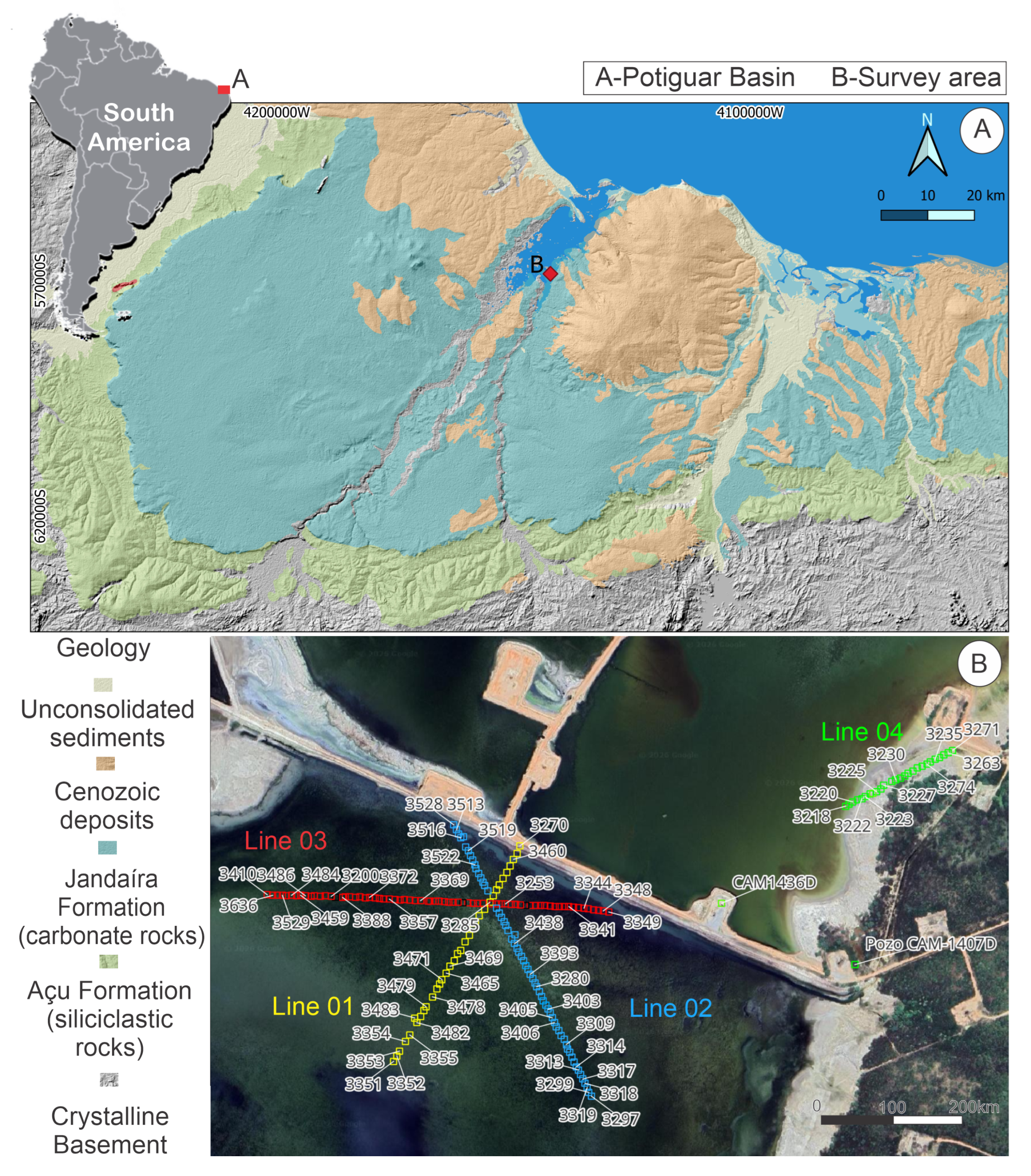
Figure 2.
Processing workflow for the extraction of P-wave reflectivity from autocorrelation functions. The flowchart outlines the sequential data processing stages applied to continuous passive seismic records. The architecture is divided into three core phases: time-domain preprocessing (raw data ingestion, segment windowing, linear/mean detrending, and data tapering); frequency-domain conditioning via Fast Fourier Transform (FFT) for Gaussian smoothing and spectral whitening; and the return to the time domain via Inverse Fast Fourier Transform (IFFT) for discrete autocorrelation calculation and final linear trace stacking.
Figure 2.
Processing workflow for the extraction of P-wave reflectivity from autocorrelation functions. The flowchart outlines the sequential data processing stages applied to continuous passive seismic records. The architecture is divided into three core phases: time-domain preprocessing (raw data ingestion, segment windowing, linear/mean detrending, and data tapering); frequency-domain conditioning via Fast Fourier Transform (FFT) for Gaussian smoothing and spectral whitening; and the return to the time domain via Inverse Fast Fourier Transform (IFFT) for discrete autocorrelation calculation and final linear trace stacking.
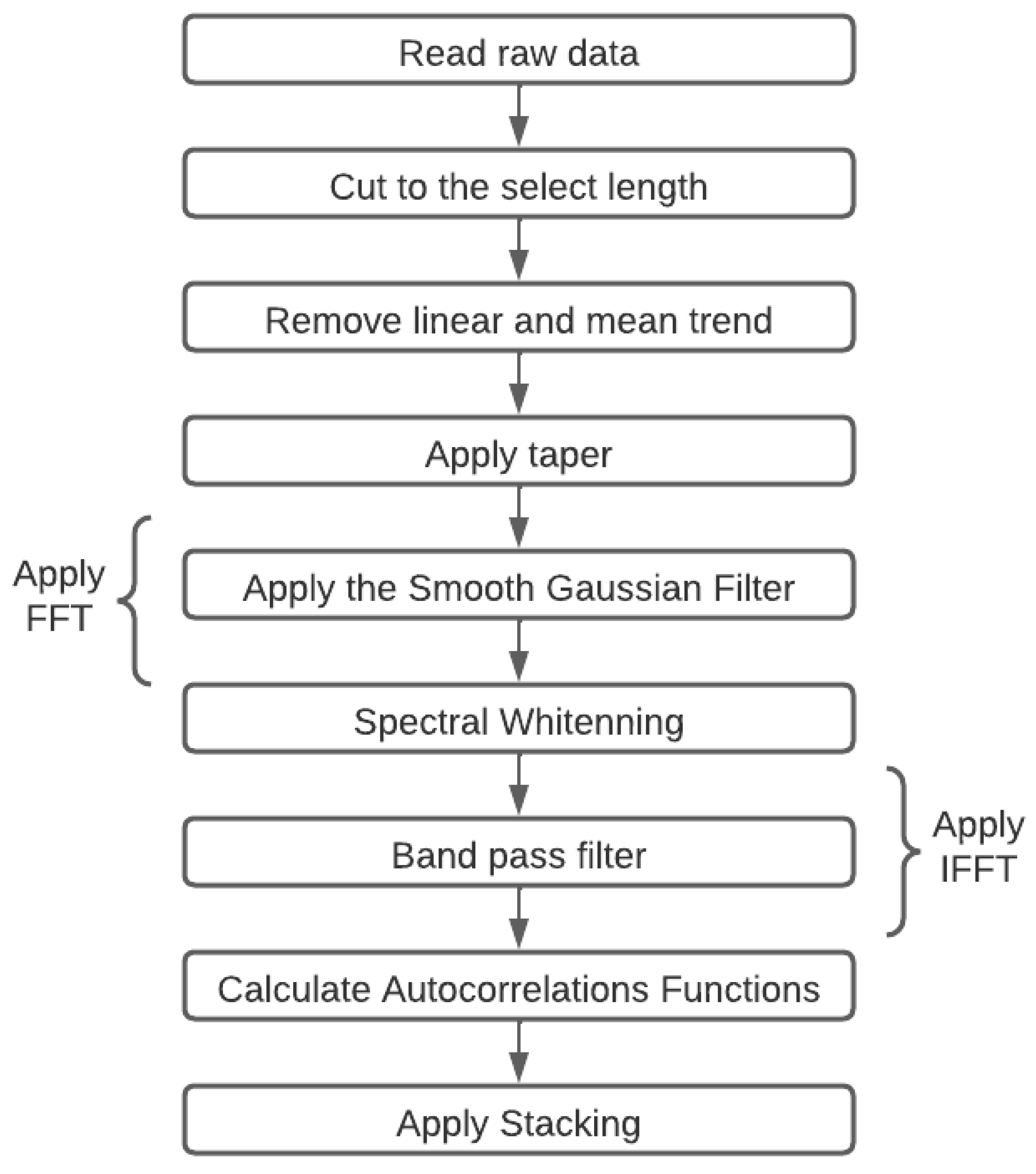
Figure 3.
Processing workflow for surface-wave retrieval and empirical Green’s function extraction via cross-correlation. The schematic shows the sequential stages optimized for processing continuous passive seismic data based on the method of Bensen et al. (2007). The processing sequence moves from raw data evaluation and linear detrending through targeted bandpass filtering. Signal conditioning is achieved by applying 1-bit temporal normalization and spectral whitening to eliminate high-amplitude transient noise and balance the frequency spectrum. The workflow concludes with classical cross-correlation computation between receiver pairs, followed by Phase-Weighted Stacking (PWS) to optimize the retrieval of coherent Rayleigh wave trains.
Figure 3.
Processing workflow for surface-wave retrieval and empirical Green’s function extraction via cross-correlation. The schematic shows the sequential stages optimized for processing continuous passive seismic data based on the method of Bensen et al. (2007). The processing sequence moves from raw data evaluation and linear detrending through targeted bandpass filtering. Signal conditioning is achieved by applying 1-bit temporal normalization and spectral whitening to eliminate high-amplitude transient noise and balance the frequency spectrum. The workflow concludes with classical cross-correlation computation between receiver pairs, followed by Phase-Weighted Stacking (PWS) to optimize the retrieval of coherent Rayleigh wave trains.
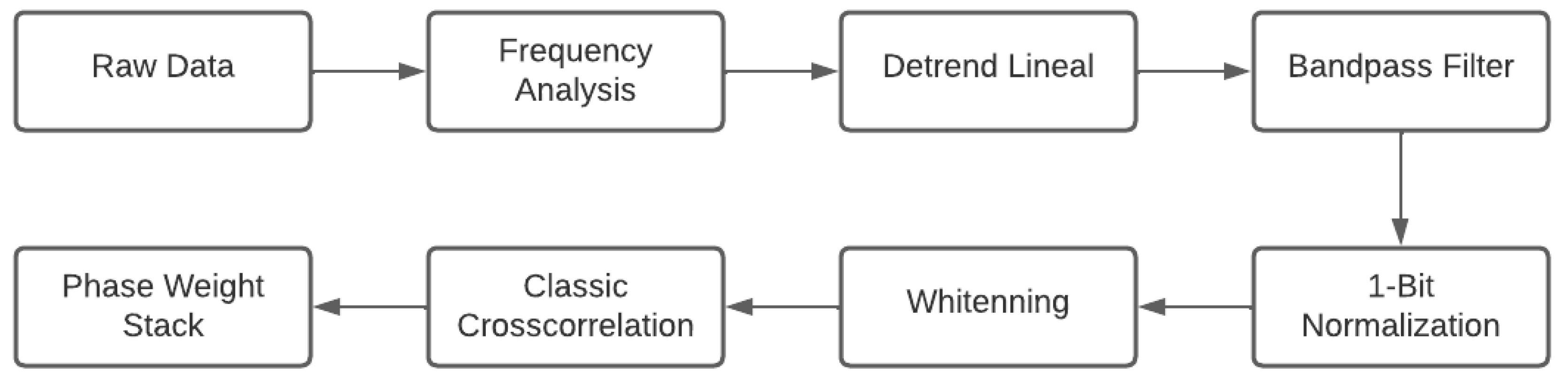
Figure 4.
Seismic imaging section of line 03. Figure a) displays the results for a frequency range between 2-16 Hz, while figures b) and c) show the seismic sections for frequency ranges between 2-20 Hz and 2-30 Hz, respectively.
Figure 4.
Seismic imaging section of line 03. Figure a) displays the results for a frequency range between 2-16 Hz, while figures b) and c) show the seismic sections for frequency ranges between 2-20 Hz and 2-30 Hz, respectively.
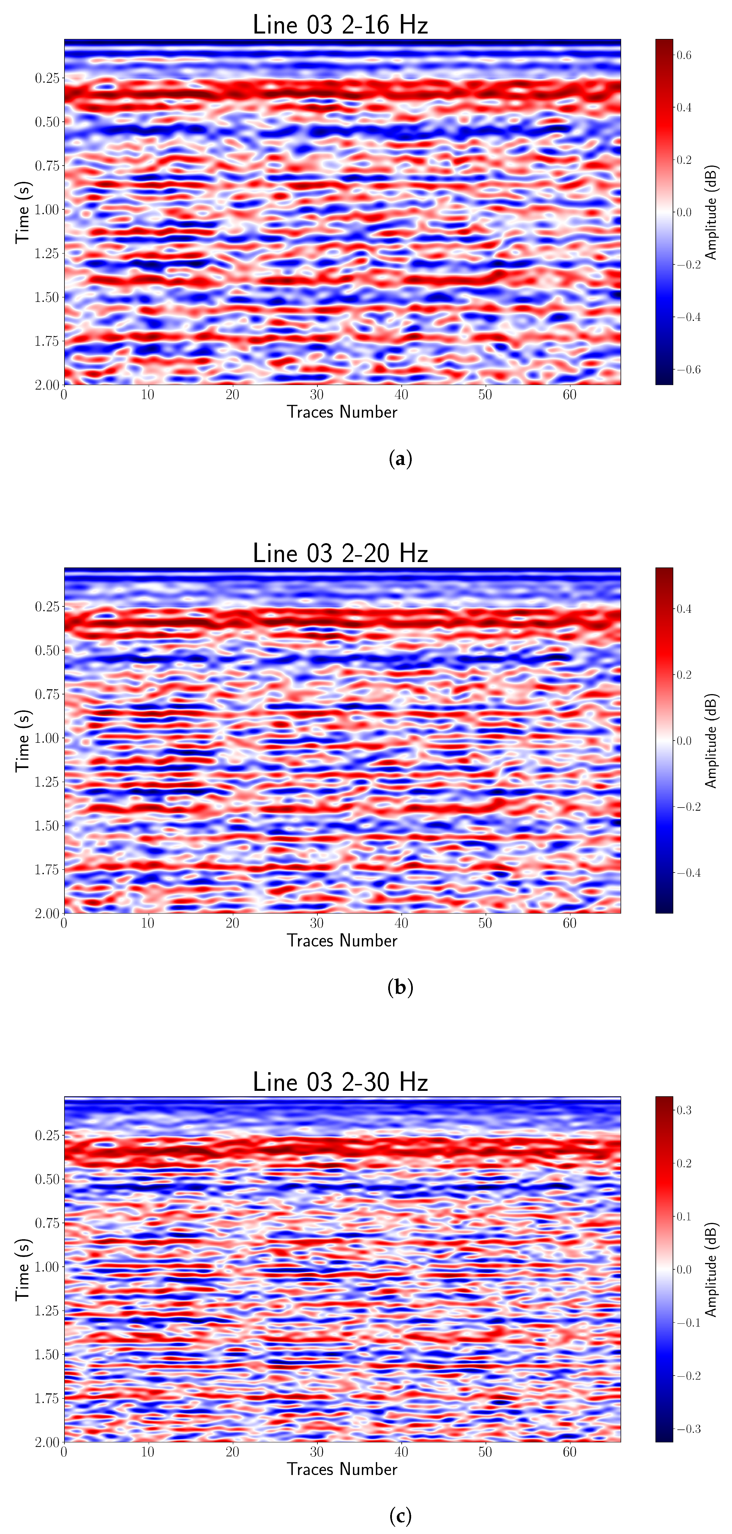
Figure 5.
Seismic imaging section of Line 01. Figure a) displays the results for a frequency range between 2-16 Hz, while figures b) and c) show the seismic sections for frequency ranges between 2-20 Hz and 2-30 Hz, respectively.
Figure 5.
Seismic imaging section of Line 01. Figure a) displays the results for a frequency range between 2-16 Hz, while figures b) and c) show the seismic sections for frequency ranges between 2-20 Hz and 2-30 Hz, respectively.
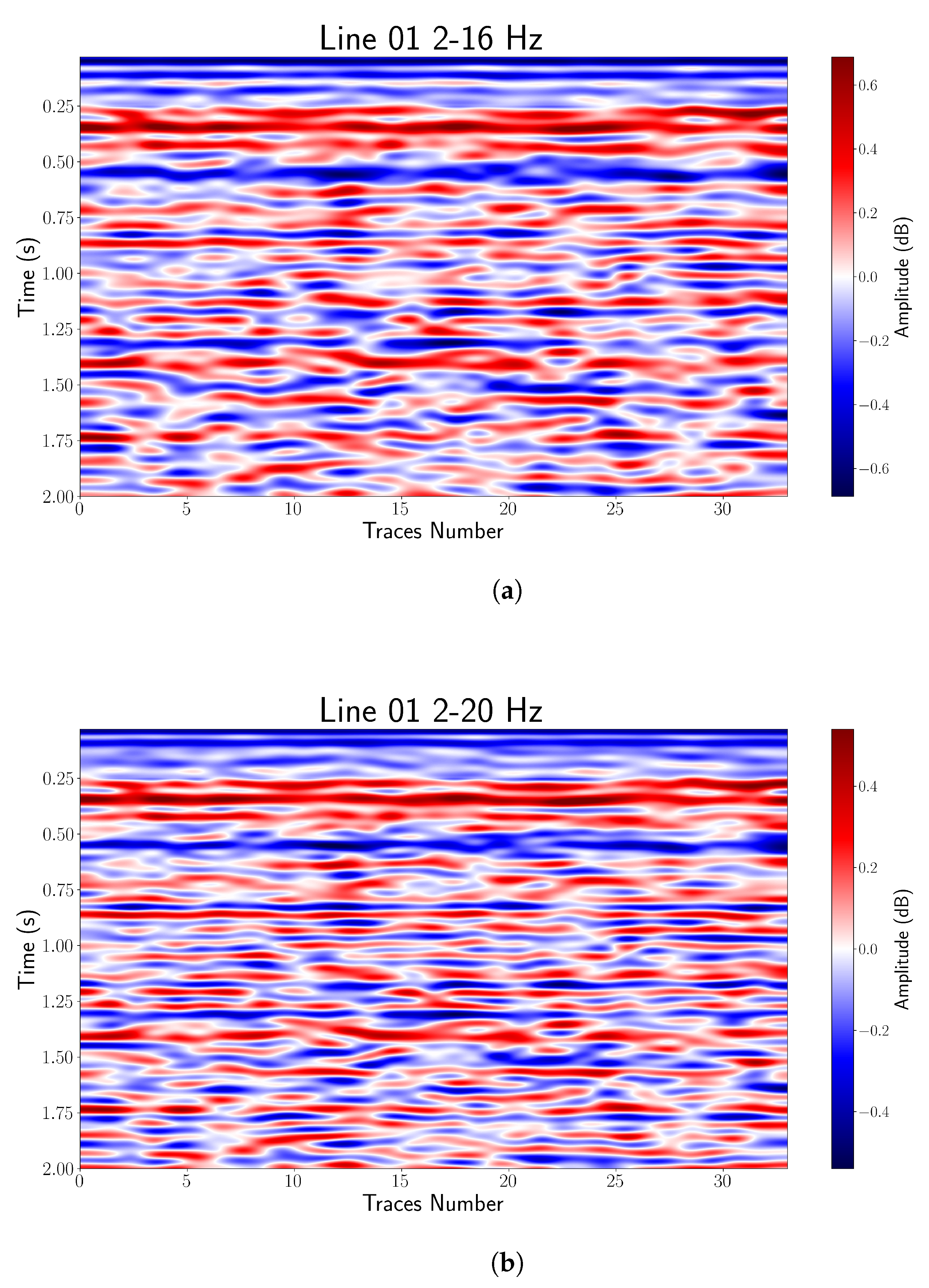
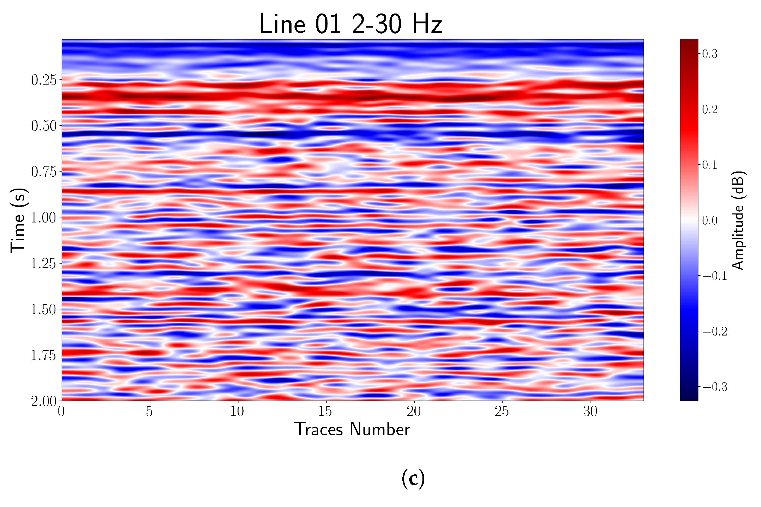
Figure 6.
Seismic section of Line 02. Figure a) displays the results for a frequency range between 2-16 Hz, while figures b) and c) show the seismic sections for frequency ranges between 2-20 Hz and 2-30 Hz, respectively.
Figure 6.
Seismic section of Line 02. Figure a) displays the results for a frequency range between 2-16 Hz, while figures b) and c) show the seismic sections for frequency ranges between 2-20 Hz and 2-30 Hz, respectively.
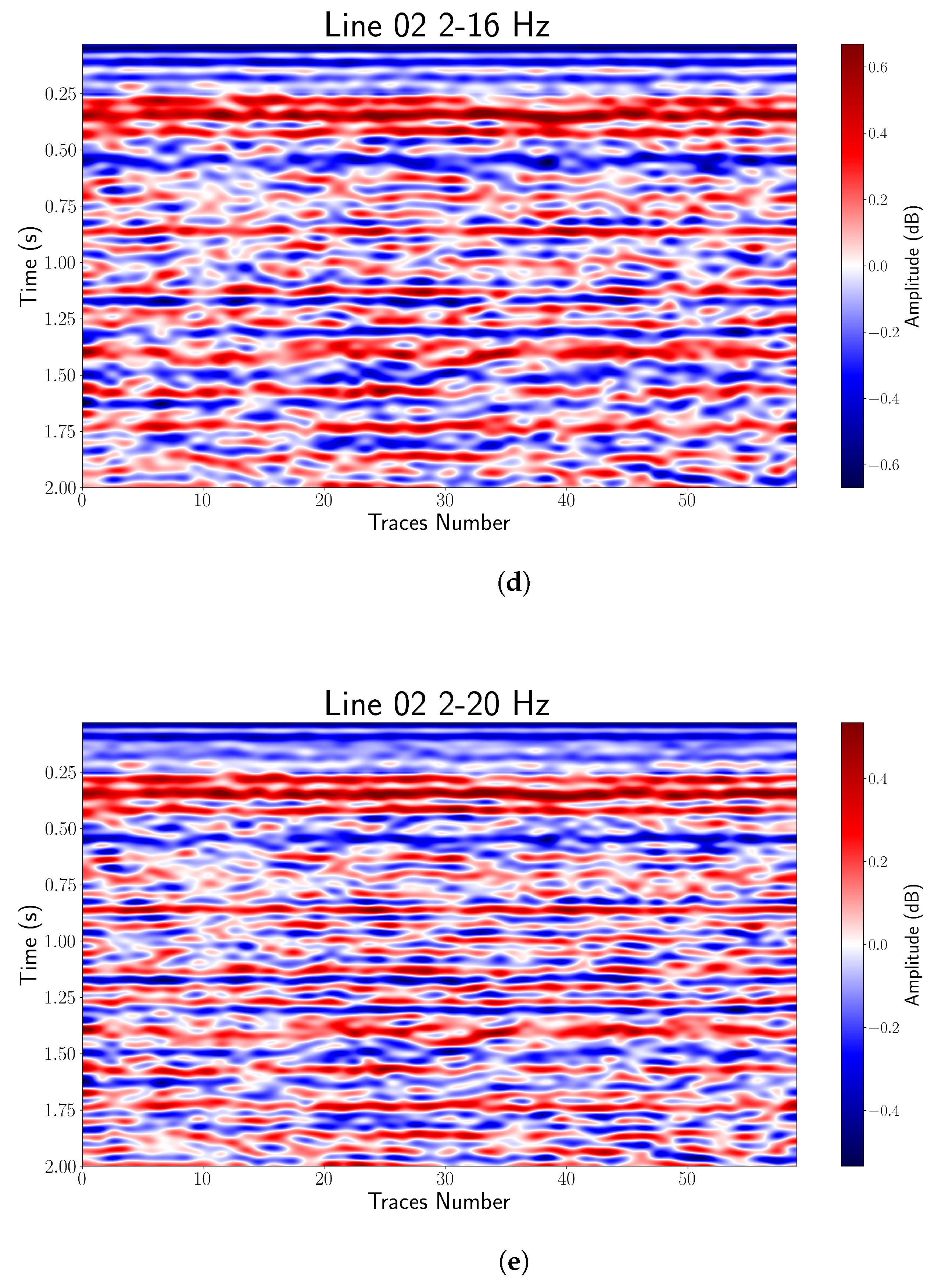
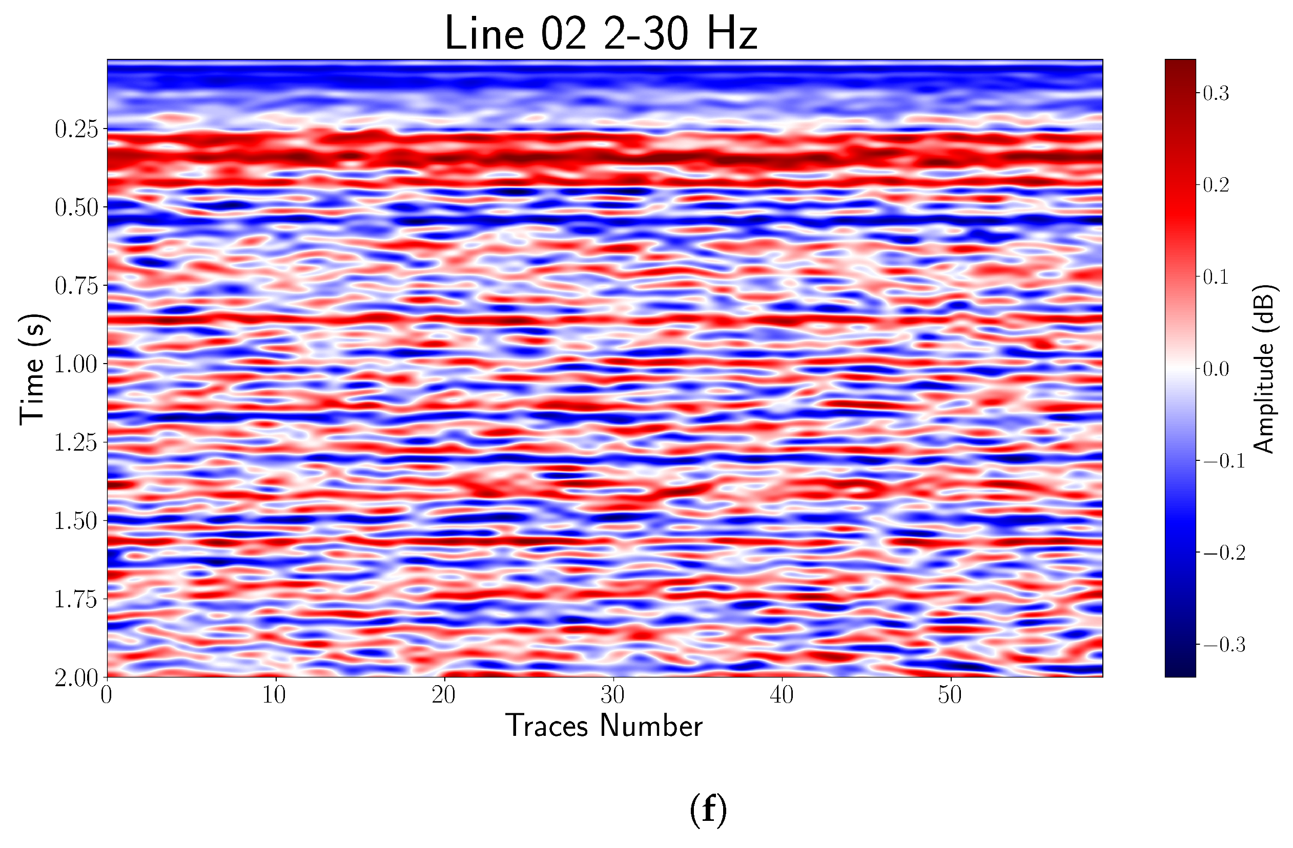
Figure 7.
Comparison between the seismic section obtained from the autocorrelation function and a seismic line located very close to the study area. Figure 7(g) corresponds to Line 02 obtained from passive seismic data, whereas Figure 7(h) highlights the main reflectors obtained. Figure 7(i) and Figure 7(j) refer to active seismic and the identification of their main reflectors, respectively.
Figure 7.
Comparison between the seismic section obtained from the autocorrelation function and a seismic line located very close to the study area. Figure 7(g) corresponds to Line 02 obtained from passive seismic data, whereas Figure 7(h) highlights the main reflectors obtained. Figure 7(i) and Figure 7(j) refer to active seismic and the identification of their main reflectors, respectively.
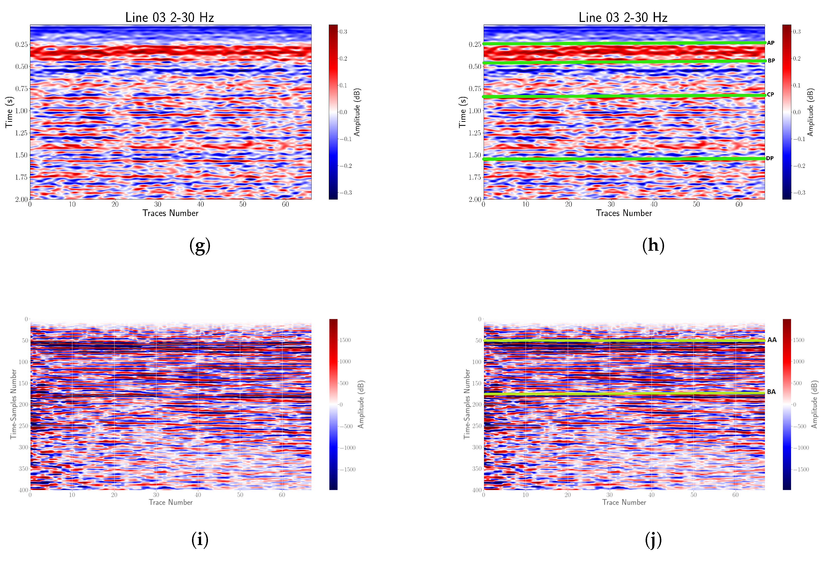

Table 1.
Geophone acquisition parameters and array geometry. Detailed breakdown of receiver line layouts, indicating total active sensor counts and station intervals (m) used during the passive monitoring survey. Numbers in parentheses indicate the count of non-functional or inactive sensors omitted from the final interferometric processing workflow.
Table 1.
Geophone acquisition parameters and array geometry. Detailed breakdown of receiver line layouts, indicating total active sensor counts and station intervals (m) used during the passive monitoring survey. Numbers in parentheses indicate the count of non-functional or inactive sensors omitted from the final interferometric processing workflow.
| Line number | Number of receivers | Spacing (m) | |
|---|---|---|---|
| Line 01 | 35(2) | 15 | |
| Line 02 | 60(1) | 10 | |
| Line 03 | 70(3) | 10 | |
| Line 04 | 26(2) | 10 |
Disclaimer/Publisher’s Note: The statements, opinions and data contained in all publications are solely those of the individual author(s) and contributor(s) and not of MDPI and/or the editor(s). MDPI and/or the editor(s) disclaim responsibility for any injury to people or property resulting from any ideas, methods, instructions or products referred to in the content. |
© 2026 by the authors. Licensee MDPI, Basel, Switzerland. This article is an open access article distributed under the terms and conditions of the Creative Commons Attribution (CC BY) license (http://creativecommons.org/licenses/by/4.0/).
Copyright: This open access article is published under a Creative Commons CC BY 4.0 license, which permit the free download, distribution, and reuse, provided that the author and preprint are cited in any reuse.


