
Submitted:
29 June 2026
Posted:
30 June 2026
You are already at the latest version
Abstract
With the continuous increase in coal mining depth in China, concealed geological structures—such as collapse columns and faults—pose a severe threat to mine safety by inducing water inrush accidents. Mine DC resistivity methods exhibit high sensitivity to the water-bearing characteristics of geological bodies but suffer from limited resolution. In contrast, mine seismic exploration offers high resolution but shows weak responses to water-rich bodies. Single-method inversion inevitably faces the issue of solution non-uniqueness. This study aims to enhance the detection accuracy of concealed structures by implementing a joint seismic-electric inversion, leveraging the complementary advantages of both methods. For the DC resistivity component, a forward model was established using the finite element method with unstructured meshes, and inversion was performed using a least-squares algorithm. For seismic exploration, forward modeling utilized curved-ray tracing, and inversion was conducted via the LSQR algorithm. Cross-gradient constraints were incorporated into the joint inversion to establish a structurally coupled framework. Numerical simulation results indicate that while single-method inversions (DC or seismic) can preliminarily identify anomalies, they are limited by issues such as anomaly diffusion and false anomalies. In contrast, the joint in-version effectively constrains the spatial extent of anomalies, accurately characterizes the morphology and location of multiple anomalous bodies, fractures, and water-conducting fault channels, and significantly reduces solution non-uniqueness. This research provides a reliable methodology for the refined detection of concealed hazard-inducing structures, offering substantial practical value for ensuring coal mine safety.
Keywords:
DC resistivity method
; seismic exploration
; joint inversion
; numerical simulation
; cross-gradient
1. Introduction
Coal mining in China is progressively extending to greater depths, where increasing geological complexity elevates the risk of water inrush accidents caused by concealed structures—such as collapse columns and faults—posing serious threats to safety and personnel. Precise characterization of the spatial distribution and water-richness of these hidden hazards is a prerequisite for scientific water hazard control and safe pressurized mining. Currently, borehole DC resistivity and seismic exploration have emerged as core techniques for detecting concealed hazards underground, owing to their complementary physical principles.
The mine DC resistivity method, based on contrasts in electrical conductivity, is highly sensitive to low-resistivity anomalies such as water-bearing bodies and fractured zones, enabling effective identification of water-rich structures in roofs and floors. However, constrained by underground observation systems and algorithmic limitations, it suffers from insufficient resolution, making it difficult to precisely delineate anomaly boundaries; this often leads to anomaly diffusion and false anomalies, particularly in scenarios with multiple coexisting targets. Mine seismic exploration, relying on seismic impedance contrasts, offers high resolution and signal-to-noise ratio, excelling at characterizing structural interfaces and rock mass integrity. Nevertheless, its response to variations in water content is weak, rendering it ineffective for distinguishing between dry and water-saturated structures. The inherent limitations of single geophysical methods result in significant non-uniqueness in data interpretation, failing to meet the demand for high-precision exploration in modern smart mines.
Joint inversion, which integrates the advantages of multiple methods to achieve data complementarity and mutual constraints, has become a key technology to overcome the bottlenecks of single-method detection. Since Vozoff and Jupp (1975) pioneered true joint inversion, related research has evolved from one-dimensional layered models to three-dimensional complex structures and from linear to nonlinear approaches [1]. Lines et al.(1988) employed the least-squares method for joint inversion and compared the merits of sequential and synchronous strategies [2]. In 1995, Hering et al(1995). proposed the first 1D joint inversion formulation for DC resistivity and seismic surface-wave data, laying the theoretical groundwork for subsequent seismic-electric inversion [3]. Kis et al.(2001) further realized the joint inversion of multiple wave types and DC apparent resistivity for 2D geological bodies [4]. Gallardo and Meju(2003) have conducted extensive systematic research in this field; their proposed cross-gradient constraint theory avoids presupposing empirical relationships between petrophysical parameters. Instead, it enhances the structural consistency of different property models to achieve joint inversion, significantly improving accuracy and reliability [5]. This method has since been widely applied in studies such as 3D joint inversion of potential field data.
In China, Wang Jialin and colleagues summarized the application conditions for joint inversion through extensive research [6]. Chen Xiao and Yu Peng introduced regularization and adaptive techniques into synchronous joint inversion, enhancing solution stability and computational efficiency [7]. Zhou Lifen employed cross-gradient theory to couple resistivity and seismic velocity data, achieving 2D synchronous joint inversion of magnetotelluric and seismic data [8]. Gao Ji and Zhang Haijiang developed a joint inversion scheme for seismic traveltime and DC resistivity data with cross-gradient constraints, effectively mitigating shadow zone issues in seismic body-wave tomography and DC resistivity imaging [9]. Peng Miao, Tan Handong et al. conducted three-dimensional joint inversion of magnetotelluric and seismic travel time data with cross-gradient constraints. The study demonstrated that joint inversion enhanced the recovery degree of deep velocity structure characteristics of the abnormal body [10].These domestic studies have confirmed the feasibility of applying cross-gradient theory to seismic-electric joint inversion. However, a critical assessment shows that existing studies primarily focus on general geophysical scenarios. Significant gaps remain regarding adaptation to the confined spaces and complex boundaries (e.g., roadway interference) of underground mines, and there is a lack of targeted research on typical hazardous structures like water-conducting collapse columns and faults. Moreover, the critical balance between inversion accuracy and computational efficiency under deep mining conditions remains unresolved. Concurrently, the advancement of intelligent mining has intensified electromagnetic interference, challenging the robustness of current methods against practical operational conditions.
The inherent complementarity between mine DC resistivity and seismic exploration provides a natural foundation for addressing the challenge of accurately detecting concealed hazardous structures. Consequently, this paper focuses on developing a mine-adapted seismic-electric joint inversion method. We aim to optimize the structural coupling constraints and inversion algorithms. Through numerical simulations based on theoretical models of various anomalies and typical disaster-inducing structures, we seek to establish a joint inversion framework suited to complex mine conditions. This work is intended to provide a reliable technical pathway for the precise detection of concealed geological hazards, thereby offering robust support for smart mine construction and safety in production.
2. Individual Inversion
2.1. Mine DC Resistivity Method
2.1.1. Forward Modeling
The forward model is constructed using the finite element method (FEM) with an unstructured triangular mesh. The computational domain is discretized into triangular elements to accurately conform to complex geological geometries and roadway boundaries in the mine environment (Figure 1) [11].
Based on the minimum energy principle of electrostatics, the boundary value problem of the potential distribution governed by partial differential equations is transformed into a variational problem [12]. Discretization yields a large sparse linear algebraic system:
where σ denotes the electrical conductivity of the subsurface medium, δ represents the Dirac delta function, n is the coordinate variable in the outward normal direction of the boundary, r is the position vector from the source point to a boundary point, Ω signifies the computational domain, and Γs, Γ∞ refer to the ground surface and subsurface boundaries, respectively.
Linear basis functions are adopted for interpolation within each triangular element. Integral results of all elements are assembled to derive the global matrix system:
where U denotes the global nodal potential vector. According to the variational extremum principle, setting the first variation of Equation (4) to zero generates the linear algebraic system:
The symmetric successive over-relaxation (SSOR) preconditioned conjugate gradient (CG) method is adopted for efficient solution. An SSOR preconditioner is constructed to improve the condition number of the stiffness matrix K. Combined with sparse matrix storage techniques, an optimized SSOR-preconditioned iterative algorithm is developed referring to the incomplete Cholesky decomposition preconditioned biconjugate gradient strategy, and the nodal potential distribution U of the study area is ultimately obtained. This solution scheme guarantees computational accuracy while significantly enhancing the solving efficiency for large-scale 3D problems.
2.1.2. Inversion Algorithm
The inversion problem is formulated as a regularized least-squares optimization problem. The objective function is established based on the Occam inversion algorithm to balance data fitting accuracy and model smoothness [13]:
where Δd is the residual vector between field observations and theoretical forward data, m denotes the model parameter vector, J represents the sensitivity (Jacobian) matrix, λ is the dynamically adjusted regularization parameter, and R signifies the model roughness matrix.
The model parameter update equation is expressed as:
In DC resistivity inversion, the root mean square (RMS) error is a critical indicator for evaluating the consistency between model responses and field measurements. It quantifies the overall deviation between theoretical calculations and observed data, providing an objective criterion for inversion reliability. The inversion convergence is defined as the relative change rate of RMS error being less than 2%, and the RMS error is formulated as:
where N is the number of observation data points, is the -th measured datum, and represents the theoretical response corresponding to the model parameters.
2.2. Mine Seismic Exploration
2.2.1. Forward Modeling
Unstructured mesh discretization is performed via Delaunay triangulation, employing squared slowness (the reciprocal of velocity squared) as the model parameter to adapt to the complex geological interfaces in the mine [14,15]. Based on Fermat’s principle of minimum traveltime, a curved-ray tracing method is utilized to simulate seismic wave propagation paths, iteratively correcting ray trajectories to align with true paths via the variational principle [16].
The governing forward equation system is expressed as:
In Eq. (9),denotes the length of the-th ray traversing the-th grid cell,represents the squared slowness of the-th cell,is the traveltime of the -th ray,is the total number of grid cells, and is the total number of rays. Solving this system yields theoretical traveltime datasets.
2.2.2. Inversion Algorithm
The LSQR algorithm (least-squares QR decomposition) is adopted to solve large sparse linear systems. By exploiting matrix sparsity, the computational load is drastically reduced, memory consumption is minimized, and numerical instability inherent in conventional least-squares methods is avoided; the algorithm exhibits linear convergence characteristics. This method is based on the Lanczos bidiagonalization process, iteratively constructing orthogonal matrices to transform the original system into bidiagonal form, subsequently solved via QR decomposition techniques [17].
The inversion objective function is formulated as:
whereis the coefficient matrix containing ray segment lengths, x denotes the squared slowness parameter vector, and b is the traveltime residual vector. The algorithm iteratively constructs orthogonal matrices and updates model parameters until the residuals decline to the observational error level and satisfy predefined accuracy criteria.
3. Joint Inversion
3.1. Joint Inversion Model
A synchronous joint multi-parameter inversion (SJIMM) framework is employed, constructing a target function that integrates a data-fitting term, a model regularization term, and a structural constraint term to achieve collaborative inversion of DC resistivity and seismic data [18]:
where the parameters are defined as follows:
: residual norm;
A: total number of independent observation datasets;
B: number of inverted petrophysical parameters;
C: number of coupling constraints between parameters;
: model parameter vector;
: regularization parameter;
: weight coefficient of the-th model constraint function;
:-th model constraint function;
: model regularization term.
When the inversion system involves only two datasets and two petrophysical parameters, the generalized joint inversion framework (Eq. (11)) simplifies to the specific form:
3.2. Structural Constraint Conditions
Cross-gradient constraints are employed to establish structural consistency between resistivity and velocity parameters, eliminating the need for presupposed empirical relationships between physical properties. This enhances inversion accuracy by strengthening the synchrony of dual property models [19]. The constraint function is expressed as:
In numerical computation, the cross-gradient function for the -th triangular mesh element is:
where, , andrepresent the cross-gradient components along the x,, and z directions, respectively, computed via the vector cross product of model parameter gradients. This design ensures synchronized variations of different petrophysical parameters at structural boundaries.
3.3. Inversion Solution Procedure
The Gauss–Newton optimization algorithm is utilized to minimize the joint inversion target function. The iterative update formula is:
where denotes the data weight matrix,is the model weight matrix,represents the reference model,is the Hessian matrix of the cross-gradient term, andis the gradient vector of the cross-gradient term.
4. Numerical Simulations
4.1. Seismic-Electric Joint Inversion Numerical Simulations
The DC resistivity method is highly sensitive to subsurface water content and fluid distribution, enabling inference of rock connectivity and fluid properties from resistivity variations. Seismic exploration responds to rock elastic moduli and density, allowing characterization of geological structures and fragmentation degrees via wave velocity and attenuation analyses. Physically realistic models and survey geometries representative of underground mine conditions are constructed. Model domains, anomaly sizes, and spatial positions are defined to match practical mining scenarios. Models are discretized via unstructured meshes to accommodate complex mine geometries and roadway boundaries, with seismic sources and geophones deployed in the working face roadways for realistic data acquisition [20]. Specifically, mine seismic wave detection employs a multi-channel seismic transmission imaging technique, with geophone arrays deployed at 10 m intervals along the roadways on both sides of the working face. The observation system adopts an equal-interval source excitation and full-array reception mode, with seismic source points arranged at 50 m intervals. A single-point excitation and full-array reception strategy is implemented to acquire high-quality seismic wavefield data, ensuring sufficient spatial coverage and angular illumination of the target zone. Mine DC resistivity detection employs a dipole-dipole configuration for data acquisition, with current (source) and potential (measuring) electrodes deployed at 10 m intervals along the sidewalls of the roadways to obtain potential difference data. This configuration provides high sensitivity to lateral resistivity variations and is well suited for detecting water-bearing structures ahead of the working face. Based on the above observation systems, numerical simulation studies are carried out separately to analyze the individual inversion effects of the two geophysical methods, providing a basis for subsequent joint inversion and comprehensive interpretation.
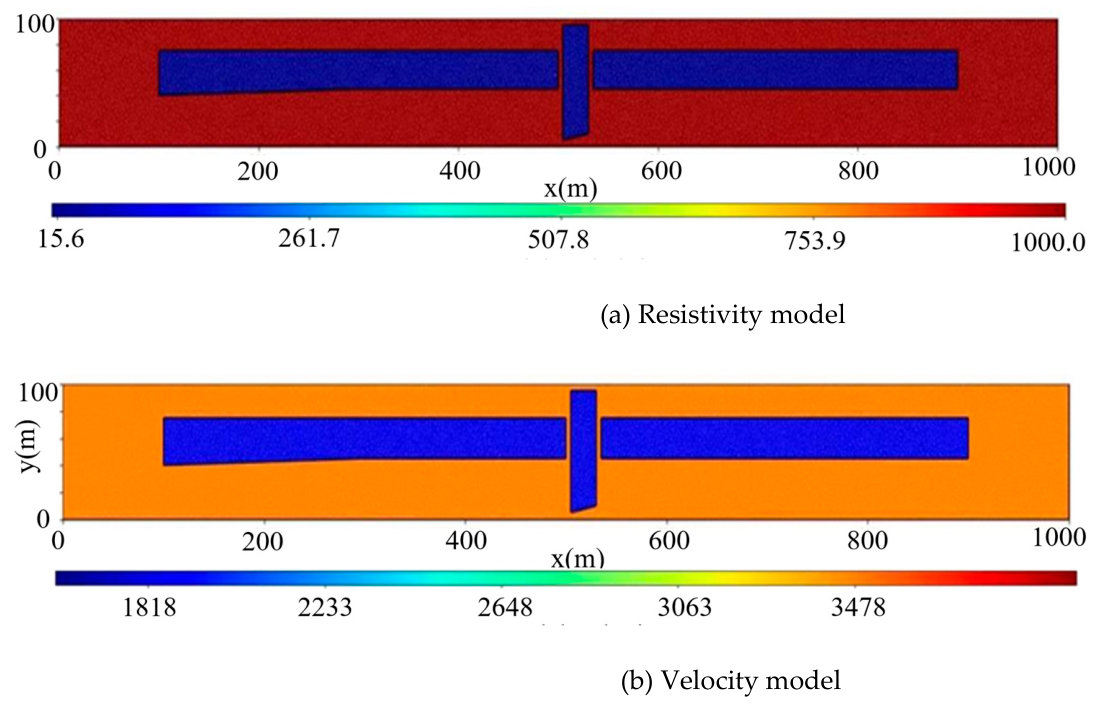
Model 1: Multiple Isolated Anomalies
Model comprises three low-resistivity anomalies embedded in a high-resistivity background and three corresponding low-velocity anomalies in a high-velocity background.
Figure 2.
DC resistivity and seismic exploration model of Model 1(Upper resistivity model, lower velocity model).
Figure 2.
DC resistivity and seismic exploration model of Model 1(Upper resistivity model, lower velocity model).
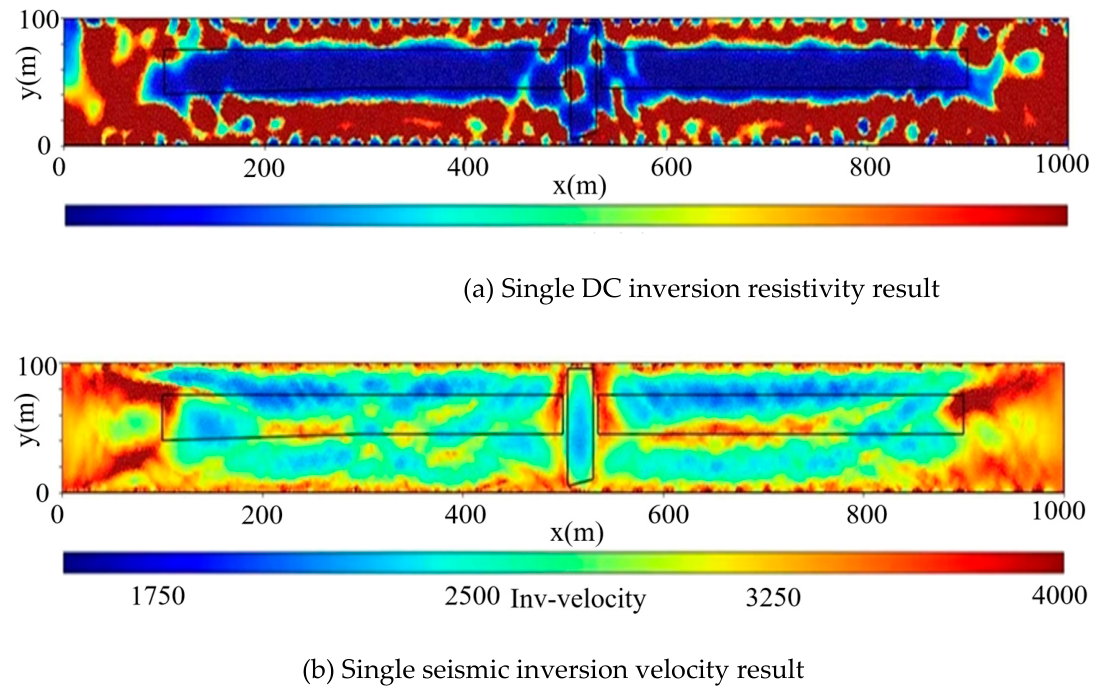
The model is discretized via unstructured triangular meshes, and synthetic DC and seismic data are generated for inversion tests. Single-method inversions reveal that resistivity-only inversion produces distorted anomaly contours, pronounced smearing, and spurious anomalies, whereas seismic-only inversion approximates the anomaly shapes but exhibits significant vertical smearing.
Figure 3.
Single inversion of model 1(Upper resistivity profile, lower velocity profile).
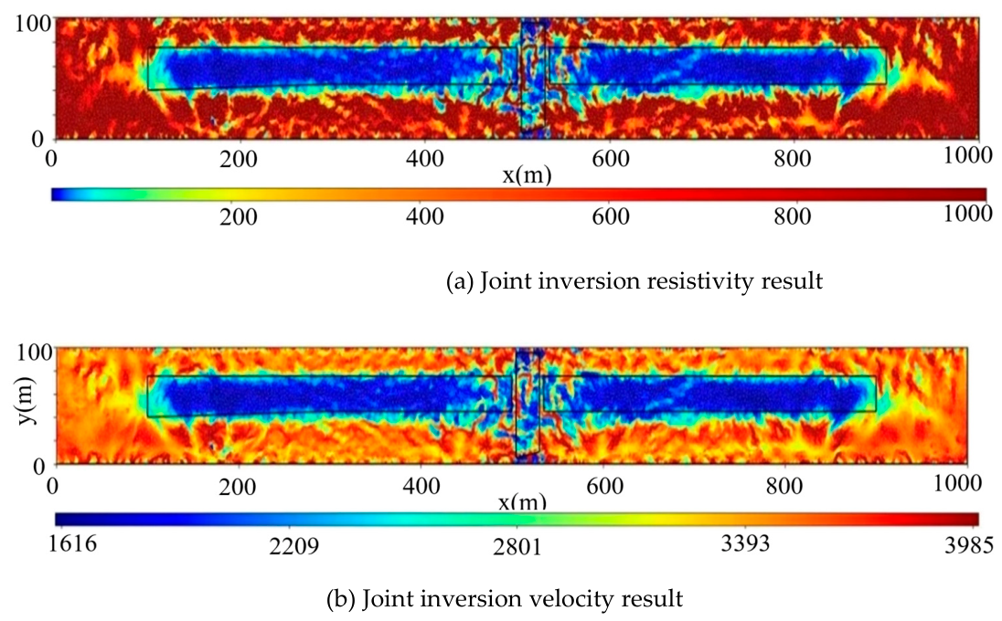
Joint inversion rectifies anomaly contours, suppresses smearing, eliminates spurious anomalies, and reconstructs anomaly spatial features with high fidelity, markedly outperforming single-method inversions.
Figure 4.
Joint inversion of Model 1.
Model 2: Fractured Water-Conducting Channel
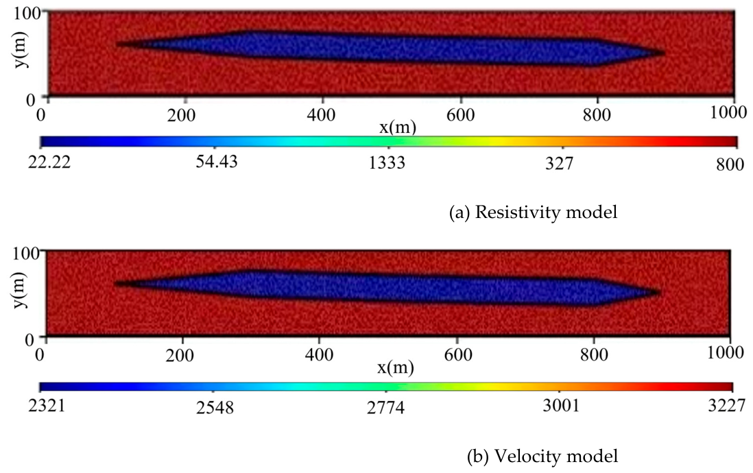
Model simulates a linear water-conducting fracture, featuring a single elongated low-resistivity anomaly and a matching low-velocity anomaly.
Figure 5.
DC resistivity and seismic exploration model of Model 2.
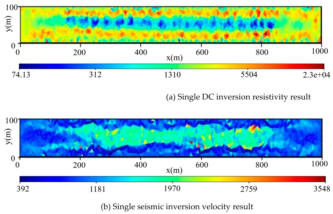
In the single resistivity inversion result, the low-resistivity anomaly appears elongated, its sharp terminations at both ends are not clearly identified, and spurious anomalies are present. In the single seismic inversion result, the sharp ends of the low-velocity anomaly are similarly not delineated accurately. (Figure 6)
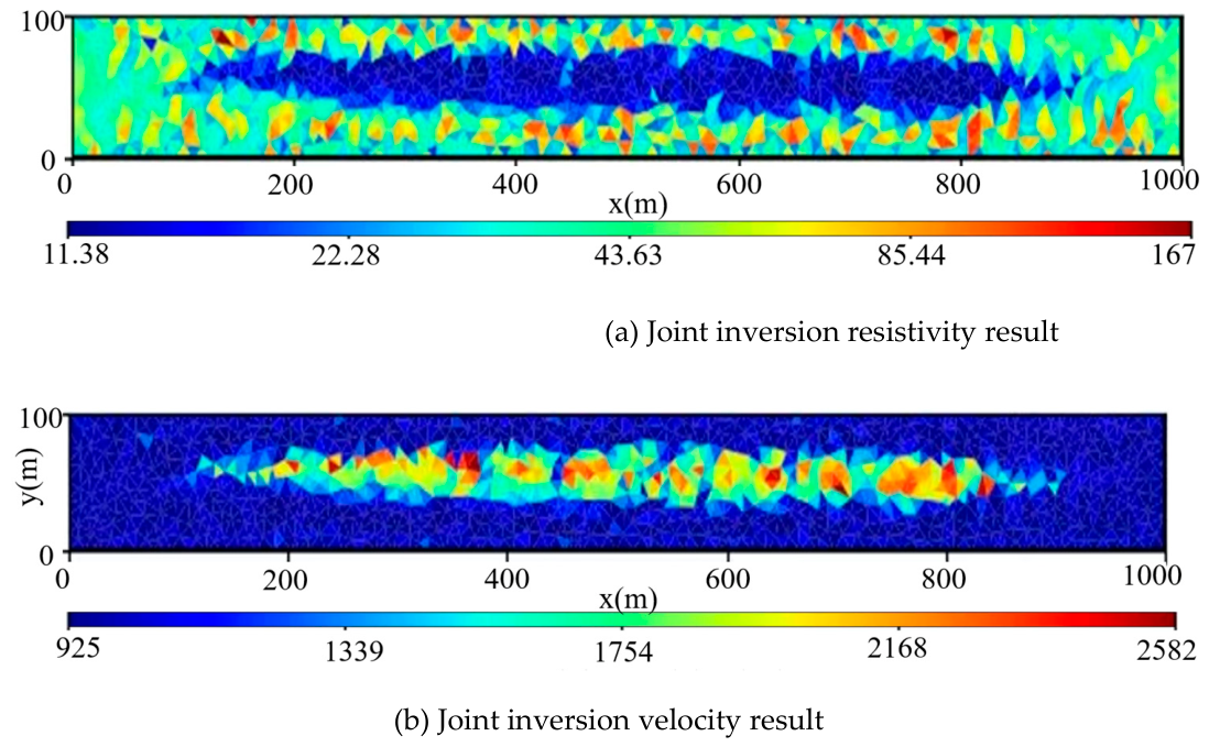
Joint inversion refines anomaly extents, accurately captures sharp channel terminations, and restrains smearing, demonstrating high precision for linear hydrogeological conduit imaging.
Figure 7.
Joint inversion of Model 2.
4.2. Summary
The seismic-electric joint inversion is implemented following a standardized workflow: data input, model initialization, unstructured mesh discretization, optimization of the joint inversion objective function via the Gauss–Newton method, and model parameter update through linear search, until the convergence criteria are satisfied.
Typical concealed hazard-inducing geological structures are constructed as model anomalies, and a comparative analysis is conducted focusing on the performance of single-method inversions (mine DC resistivity method and mine seismic exploration) versus seismic-electric joint inversion. The comparison demonstrates that by integrating multiple geophysical datasets, joint inversion effectively reduces the solution non-uniqueness inherent in single-method inversions and improves the accuracy and reliability of inversion results.
5. Conclusions
This study addresses the limitations of low resolution and high non-uniqueness inherent in single geophysical methods for detecting concealed hazardous structures in underground mines. By combining theoretical derivation, algorithm development, and numerical validation, we establish a comprehensive seismic–electric joint inversion framework. The main conclusions are summarized as follows.
(1) Single-method inversion frameworks tailored to mining conditions have been developed. For the DC resistivity method, we couple unstructured-mesh finite-element forward modeling with Occam-style regularized inversion, which reliably reconstructs the positions and resistivity parameters of anomalous bodies. For the seismic method, we adopt curved-ray forward modeling combined with the LSQR algorithm, which accurately images velocity anomalies. These frameworks lay a solid foundation for the subsequent joint inversion.
(2) A cross-gradient-constrained seismic–electric joint inversion scheme has been formulated. The scheme unifies the data-fitting term, regularization term, and cross-gradient term within a single objective function. By enforcing structural consistency between the resistivity and velocity models without assuming any empirical petrophysical relationship, the proposed scheme effectively suppresses spurious anomalies and image smearing, thereby improving the reliability of the inverted solutions.
(3) The effectiveness of the joint inversion has been verified through numerical experiments on representative mining scenarios, including multiple isolated anomalies, fractured water-conducting channels, and water-bearing faults. Compared with the single-method inversions, the proposed approach substantially improves the morphological reconstruction of anomalies, eliminates spurious features, and reduces solution non-uniqueness, offering a practical tool for the precise detection of concealed hazard-inducing structures in coal mines.
References
- Vozoff, K.; Jupp, D.L.B. Joint Inversion of Geophysical Data [J]. Geophys. J. R. Astron. Soc. 1975, 42, 977–991. [Google Scholar] [CrossRef]
- Lines, L.R.; Schultz, A.K.; Treitel, S. Cooperative inversion of geophysical data [J]. Geophysics 1988, 53(1), 8–20. [Google Scholar] [CrossRef]
- Hering, A.; Misiek, R.; Gyulai, A.; et al. A joint in-version algorithm to process geoelectric and surface wave seismic data. Part I: basic ideas1 [J]. Geophys. Prospect. 1995, 43(2), 135–156. [Google Scholar]
- Kis, M.; Gyulai, A.; Ormos, T.; et al. Joint inversion of Love and Rayleigh wave group velocities, re-fraction traveltimes and DC apparent resistivities measured above 2D geological structures [J]. Publ. Univ. Miskolc Ser. A Min. Geotechnol. 2001, 59, 23–38. [Google Scholar]
- Gallardo, L.A.; Meju, M.A. Characterization of heterogeneous near-surface materials by joint 2D inversion of dc resistivity and seismic data [J]. Geophys. Res. Lett. 2003, 30(13). [Google Scholar]
- Yu, P.; Zhang, L.; Wang, J.; Wu, J.; et al. Determination of Physical Property Parameters Structure in Middle Guizhou Uplift by Joint Inversion of Magnetotelluric, Seismic, Gravity and Magnetic Data [J]. J. TONGJI Univ. Nat. Sci. 2008, 36(3), 7. [Google Scholar] [CrossRef]
- Chen, X.; Yu, P.; Zhang, L.-L.; Li, Y.; Wang, J.-L. Adaptive regularized synchronous joint inversion of MT and seismic data [J]. Chin. J. Geophys. (in Chinese). 2011, 54(10), 2673–2681. [Google Scholar] [CrossRef]
- Zhou, L. Two Dimensional Joint Inversion of MT and Seismic data [D]; China University of Geo-sciences (Beijing), 2012. [Google Scholar]
- Gao, J.; Zhang, H.-J. Two-dimensional joint inversion of seismic velocity and electrical resistivity using seismic travel times and full channel electrical measurements based on alternating cross-gradient structural constraint [J]. Chin. J. Geophys. (in Chinese). 2016, 59(11), 4310–4322. [Google Scholar] [CrossRef]
- Peng, M.; Tan, H.-D.; Jiang, M.; Qian, H.; Tan, J.-Y. Three-dimensional joint inversion of magnetotelluric and seismic travel time data with cross-gradient constraints [J]. Chin. J. Geophys. (in Chinese). 2013, 56(8), 2728–2738. [Google Scholar] [CrossRef]
- Wang, Z.; Wang, C.; Fang, S.-N. Constraint inversion of three-dimensional bore-hole-to-surface resistivity based on unstructured finite element [J]. Geophys. Geochem. Explor. 2022, 46(6), 1431–1443. [Google Scholar] [CrossRef]
- Wu, X.-P.; Xu, G.-M. STUDY ON 3-D RESISTIVITY INVERSION USING CONJUGATE GRADIENT METHOD [J]. Chin. J. Geophys. (in Chinese). 2000, 43(03), 420–427. [Google Scholar]
- Pelton, W.H.; Rijo, L.; Swift, C.M., Jr. Inversion of two-dimensional resistivity and induced-polarization data [J]. Geophysics 1978, 43(4), 788–803. [Google Scholar] [CrossRef]
- Wang, X.; Li, Y.; Wang, P.; Wang, X.; Lü, M. Estimation and application of micro-seismic data SRV based on improved Delaunay triangulation algorithm [J]. Prog. Geo-Phys. 2021, 36(2), 689–695. [Google Scholar] [CrossRef]
- Zhao, B.; Meng, X.-H.; Hou, J.-Q. Building and Visualization of 3D Seismic Model. Earth Sci. 2007, 32(4), 549–553. [Google Scholar]
- Thurber, C.H.; Ellsworth, W.L. Rapid solution of ray tracing problems in heterogeneous media [J]. Bulle-Tin Seismol. Soc. Am. 1980, 70(4), 1137–1148. [Google Scholar]
- Lee, E.J.; Huang, H.; Dennis, J.M.; et al. An optimized parallel LSQR algorithm for seismic tomography [J]. Comput. Geosci. 2013, 61, 184–197. [Google Scholar]
- Liu, J. Dissertation for master’s degree East China University of Technology [D]; EAST CHINA UNIVERSITY OF TECHNO-LO-GY, 2023. [Google Scholar] [CrossRef]
- Gallardo, L.A.; Meju, M.A. Characterization of heterogeneous near-surface materials by joint 2D inversion of dc resistivity and seismic data [J]. Geophys. Res. Lett. 2003, 30(13). [Google Scholar]
- Dell’ Aversana, P. Self-Aware Joint Inversion of Multidisciplinary Geophysical Data in Mineral Exploration Using Hyperparameter Self-Adjustment: A Preliminary Study. Minerals 2025, 15, 623. [Google Scholar] [CrossRef]
Figure 1.
unstructured triangular mesh.
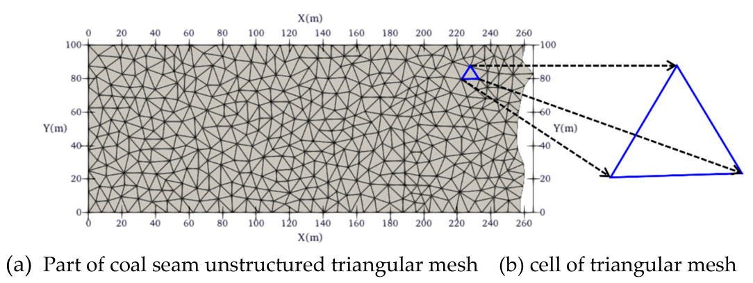
Figure 6.
Single inversion of model 2.
Disclaimer/Publisher’s Note: The statements, opinions and data contained in all publications are solely those of the individual author(s) and contributor(s) and not of MDPI and/or the editor(s). MDPI and/or the editor(s) disclaim responsibility for any injury to people or property resulting from any ideas, methods, instructions or products referred to in the content. |
© 2026 by the authors. Licensee MDPI, Basel, Switzerland. This article is an open access article distributed under the terms and conditions of the Creative Commons Attribution (CC BY) license.
Copyright: This open access article is published under a Creative Commons CC BY 4.0 license, which permit the free download, distribution, and reuse, provided that the author and preprint are cited in any reuse.


