
Submitted:
25 June 2026
Posted:
29 June 2026
You are already at the latest version
Abstract
There has been significant interest in the quantification of statistical evidence. This paper presents a statistical philosophy focused on quantifying statistical evidence derived from data, rather than following the traditional approach of presenting statistical methodology. Our focus will be on the reasoning underlying the methods, offering a fresh development of several familiar statistical approaches. We will also illustrate how a simple example requires considerably more detail. Our paper explores additional questions that analysts should pursue. We examine issues related to the determination of sample size, stopping rules, multiple hypotheses, and how effect sizes impact the quantification of statistical evidence.
Keywords:
sample size determination
; stopping rules
; multiple hypotheses
; effect sizes
1. Introduction
This paper presents a statistical philosophy that is focused on the quantification of evidence derived from observed data. The format of the paper departs from traditional presentations of statistical methodology. Our focus will be on the reasoning underlying the methods, offering a fresh development of several familiar statistical approaches. In particular, our development will eschew the notion that a null hypothesis is formulated merely to be rejected and will eschew the notion that type I and type II error probabilities are meaningful measures of evidence. Rather, we will conceptualize a hypothesis as a statistical model, with that hypothesis being judged according to its capacity to provide an accurate prediction. The remainder of this study is structured to systematically bridge frequentist and Bayesian perspectives on evidence. We begin in Section 2 by evaluating the p-value’s role as a metric for statistical evidence, followed by an exposition of the Likelihood Principle in Section 3 to establish a theoretical foundation. Section 4 examines the inferential implications of the likelihood ratio, which provides the necessary framework for Section 5 to formally link p-values with Bayes factors. After detailing the core properties of Bayes factors in Section 6, the paper concludes in Section 7 with a discussion on the versatile and often underestimated utility of p-values in broader hypothesis testing contexts.
2. P-Value as a Measure of Evidence
The p-value is a widely used tool for statistical inference. Nevertheless, the role of the p-value in formulating scientific conclusions is often misused. In this section, we shall elucidate how the p-value is optimally interpreted as a measure of evidence.
2.1. Statistical Evidence
We can say that data favor a hypothesis when that hypothesis provides a reasonable explanation for what has occurred. For example, let us consider a population of students in a school. For the general population, IQ scores follow a normal distribution with mean 100 and standard deviation 15. We may be interested in testing the hypothesis that IQ scores in the student population are distributed the same as in the general population.
To test the hypothesis that the mean IQ score for the student population matches the general population, a random sample of 25 students is selected and their IQ scores are measured.
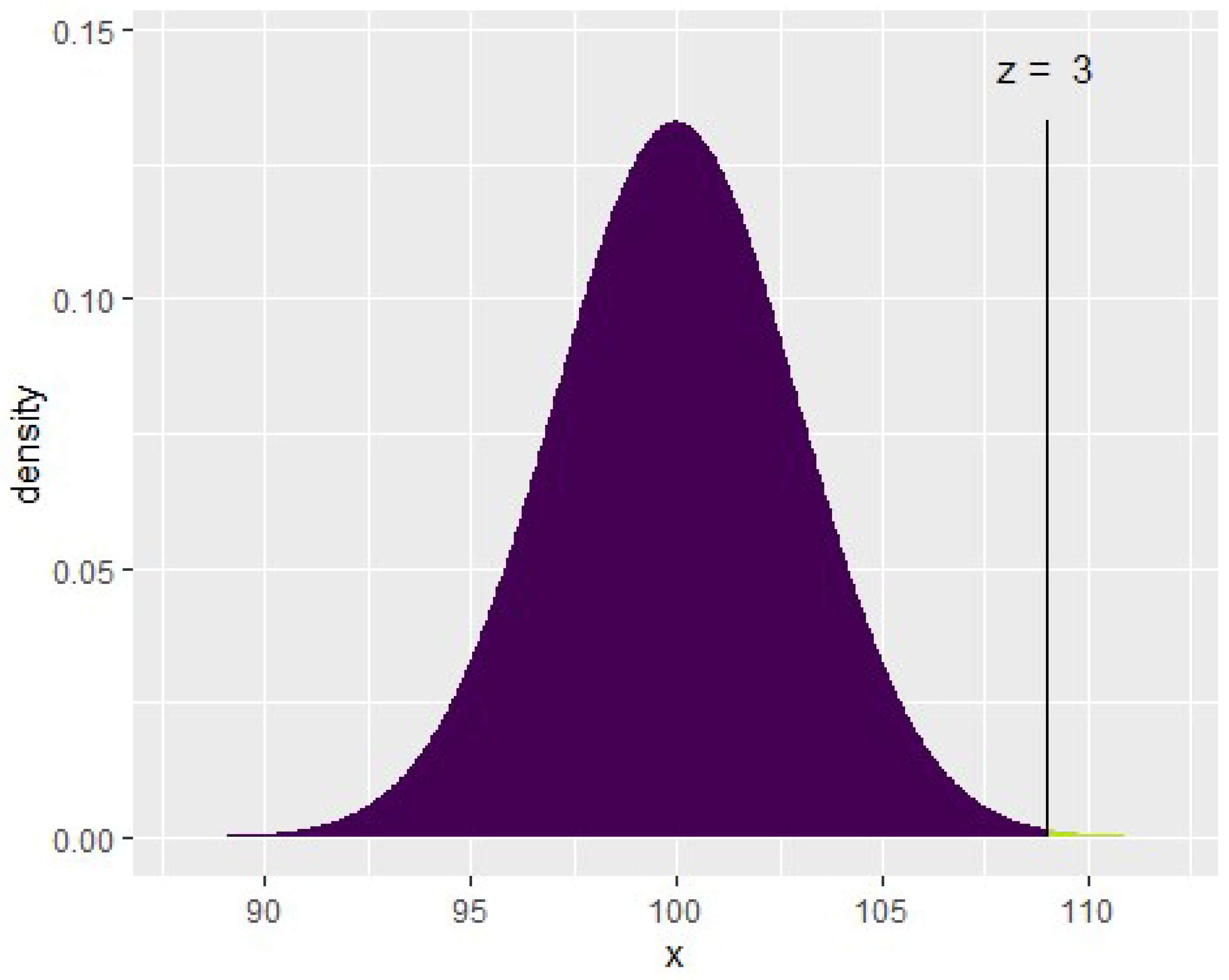
Let x denote the sample mean IQ. If the hypothesis is correct, we predict that x will be generated from a normal distribution with mean and The observed data is then compatible with the hypothesis when the sample mean x occurs in a region of high probability under the predictive distribution.
Conversely, the data provides evidence against a hypothesis when what has been observed deviates from what has been predicted. We would not predict data x in the tail region of low probability if the hypothesis were true. Observing such data would provide evidence against the hypothesis. The further into the tail, the more our data deviates from the predictive distribution, and the stronger the evidence against the hypothesis becomes. Thus, a tail probability calculation would serve as a measure of evidence. Data incompatible to the hypothesized distribution is characterized by a small p-value.
Figure 1.
Normal distribution for the general population.
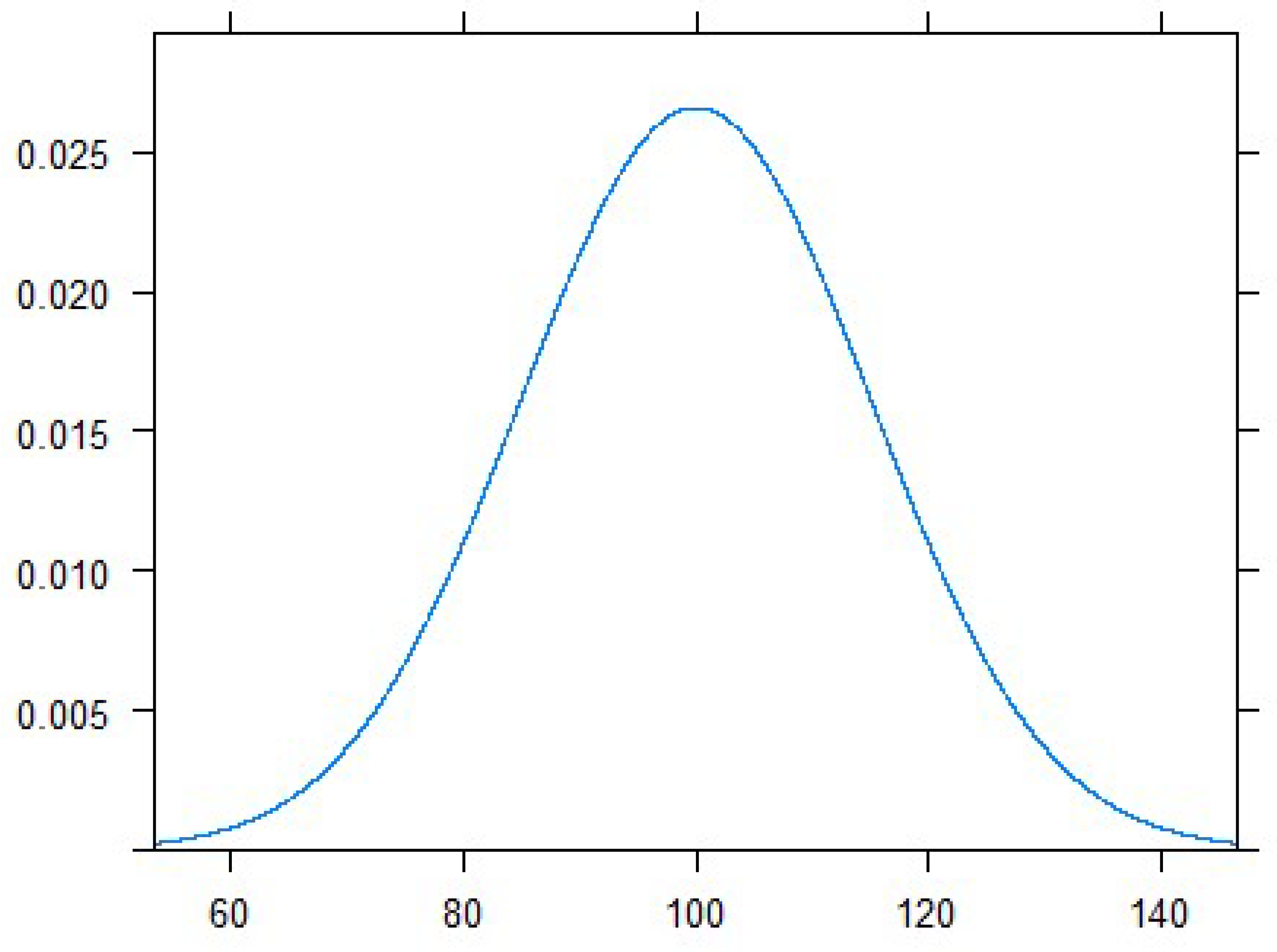
For our example, suppose we observe as the sample mean IQ score for the students. The p-value will be calculated as the tail probability, p-value .
Figure 2.
Predictive distribution and p-value calculation.
2.2. Evidence Versus Belief
Scientific evidence differs from scientific belief. A strong degree of belief is not built until multiple sources of evidence support or contradict a hypothesis. Since belief emerges from multiple studies and multiple researchers, the language for disseminating an advancement of scientific knowledge is the language of evidence. Therefore, quantification of evidence represents a core principle in statistical science.
The p-value represents a probabilistic measure of evidence, but not a probabilistic measure of belief. One must avoid the desire to interpret p as the probability that the hypothesis under examination is true. However, this leaves open the question of how to represent a p-value scale of evidence. Fisher recommended the scale displayed in Table 1. See [2] for further discussion.
The Fisher scale appears to be consistent with common p-value interpretations. In our example, we can assert there is between strong and overwhelming evidence against the hypothesis that the distribution of student IQ scores aligns with the general population.
3. The Likelihood Principle
A measure of evidence is said to satisfy the likelihood principle if the measure depends solely on the observed data and not on the experimental plan. The argument supporting the likelihood principle is that evidence measures should depend exclusively on the relevant information contained in the experimental results and not on the experimenter’s thoughts and intentions. The name derives from the fact that an evidence measure must depend exclusively on the likelihood function to satisfy the likelihood principle.
3.1. P-Value and Sampling Distribution
Since a p-value is computed based on the sampling distribution derived from the hypothesis being tested, the p-value as a measure of evidence depends on the experimental plan. Let us see with an example.
Consider a scientist investigating binomial probability . Suppose is the probability that an experimental drug leads to a successful patient outcome. The goal is to test the hypothesized probability . In the experimental study, 12 subjects are observed with 3 successes. To quantify the evidence from the experiment, we look to compute a p-value. If the experimental plan were to sample 12 subjects, the p-value would be computed based on the binomial distribution. The lower tail probability is computed for
as
giving the two-tail p-value as
Using the Fisher scale, the evidence against the hypothesized probability of success is unremarkable. But instead of a predetermined sample size , suppose that the experimenter’s intention was to sample until successes were observed. Under this scenario, the p-value is computed based on the negative binomial distribution. The upper-tail probability is computed for as
giving the two-tail p-value as
Now, we have evidence (borderline to moderate based on the Fisher scale) against the hypothesized success probability. Equivalent hypotheses, tested from equivalent data, reach different levels of evidence as measured by the p-value. The computation of the p-value is not invariant to the sampling distribution, even though the experimental plan seems like it should be unrelated to the evidence provided from the observed data.
3.2. The Likelihood Ratio Statistic
The development of an evidence measure which does satisfy the likelihood principle proceeds as follows. Let denote the likelihood as a function of an unknown parameter . For simplicity, we take the single parameter case. Nuisance parameters and parameter vectors can be handled with slight adjustments to the development. Let denote the maximum likelihood estimate. We consider the problem of testing the hypothesis under the likelihood inference framework. Define the likelihood ratio as
Then . As decreases, the data evidence against the hypothesis increases. In this sense, provides a measure of evidence against the hypothesis in the same spirit as a p-value. However, as an evidence measure satisfies the likelihood principle.
We return once more to the problem of testing the success probability . The likelihood ratio is invariant to the sampling distribution. So, the measure of evidence is the same whether the data comes from a binomial or negative binomial.
Suppose Then
Suppose Then
In either case, we write the likelihood ratio as
where the sample proportion is the maximum likelihood estimate. For testing with observed data , , we compute and
Adherence to the likelihood principle through the use of the likelihood ratio statistic, provides a measure of evidence which is a function only of the observed data. We can say the data supports the hypothesized success probability at about of the level of support to the maximum likelihood estimate. Although we were successful in creating a measure of evidence that satisfies the likelihood principle, we have lost the familiarity of interpreting evidence on a p-value scale.
Neath [5] established a connection between the p-value evidence scale and a likelihood ratio scale. From Table 2, we can say the strength of evidence against the hypothesized success probability is between borderline and moderate, no matter whether the experimenter planned binomial sampling or negative binomial sampling.
3.3. P-Value and Likelihood Ratio Under Censored Data
The p-value as a measure of evidence depends on the experimental plan. Thus, the computation of the p-value depends on the plan for censoring data regardless of whether the data observed was actually censored or not. Let’s see this with an example based on an idea from [1].
An experimenter is interested in the temperature of a particular surface. Available for performing the experiment is a device for measuring surface temperature. The device involves measurement error. The reading is distributed where is the actual temperature. Suppose that it is hypothesized that the actual surface temperature is . The device returns a reading of . A p-value is then computed based on a normal distribution. The lower tail probability is computed for as
giving the two tail p-value as
The evidence against the hypothesized temperature is only borderline on the Fisher scale.
The experimenter is happy to have an answer. The next day, he notices that the device is broken and returns a truncated value whenever the temperature measurement exceeds . Now it is the case that a p-value should be computed based on a truncated normal distribution. The lower tail probability based on the observed reading is computed to be as before. However, evidence against the hypothesized temperature can only arise for . So the p-value based on the truncated normal is one-sided, giving . The evidence against the hypothesized temperature has increased after learning that the device was broken. A quantification of evidence based on the p-value depends not on the observed data alone, but also on the irrelevant question of whether the device is working for potential readings that were not observed. The experimenter is now confused by the results.
Let’s investigate a measure of evidence which does satisfy the likelihood principle. The likelihood function for this problem is based on a truncated normal distribution. We can write the likelihood in two parts, depending on whether we observe or the truncated value of
Since we observed , we have
Since is the maximum likelihood estimate,
So , and the evidence against the hypothesized temperature is borderline as we saw initially. The experimenter is happy once again to have an answer that makes sense.
4. Consequences of the Likelihood Principle
In the last section, we saw examples where the likelihood ratio statistic provides what seems to be a more relevant measure of evidence than that which was provided by the p-value approach. In this section, we look at some consequences of adhering to the likelihood principle that may not be satisfactory.
4.1. Testing Multiple Hypotheses
In the previous sections, we considered problems where a single hypothesis is being tested. Now, let’s consider the problem of testing multiple hypotheses, For example, it may be that we are testing several medical treatments, where each treatment effect is represented in its own hypothesis.
Suppose we observe statistics for each of the M tests. Because we are testing multiple hypotheses, our focus may be on those results providing the strongest evidence. For example when testing multiple treatments, our focus would naturally be on those treatments offering the strongest evidence of an effect. In measuring evidence using the p-value, we must take note of the experimental plan. When the focus is on the test featuring the strongest evidence, then the focus is on the most extreme test result. The p-value is then computed based on the distribution for , and not on the distribution as it would be for testing a single hypothesis. We will compute the p-value for the distribution on through simulation. Figure 3 below shows the plots of some predictive distributions for multiple testing. Note how the distribution shifts to larger values as the number of tests performed increases.
Our interest is on how evidence strength for the landmark values on the Fisher scale change as the number of hypotheses being tested increase. Table 3 summarizes the results.
Remember that a p-value is based on how the observed data conforms to the predictive distribution derived from the hypothesis being tested. In our case here, the predictive distribution on is derived from multiple hypotheses, under the model where all stated hypotheses are true. The evidence for observing large Z diminishes in the sense that it becomes more probable to observe large Z for at least one of the multiple tests being considered. For example, suppose medical treatments are being tested simultaneously, and that is observed. From Table 3, we see is the computed p-value. The evidence against the model where all stated hypotheses are true is unremarkable as it is not unlikely to observe a Z as large (or larger) for at least one of the tests.
Let us now consider a measure of evidence based on the likelihood ratio statistic. Remember that an evidence measure satisfying the likelihood principle does not depend on the experimental plan. Thus, the evidence against the hypothesis will be the same no matter what other hypotheses are under consideration. In our example, the evidence against the hypothesis where was observed is interpreted as strong evidence on the likelihood ratio scale. The likelihood ratio measure of evidence gives a very different interpretation than the p-value measure. So we have two very different measures of evidence. Unlike the examples from the previous chapter, it is not so clear which measure is preferable.
Let us think again about testing several medical treatments. For treatments being studied, it would not be unlikely for a statistic from one of the treatments to be as large, or larger than the observed Under this argument, evidential support for a treatment effect somewhere among the medical treatments being studied is lacking. But we did observe for testing one of the treatment effects. This should indicate evidence in favor of an effect for that specific treatment. Under the likelihood principle, a measure of evidence should depend on the data observed (here, ), and not on whether it was the experimenter’s intention to test other hypotheses.
We can reach an agreement between the two arguments by noting that the p-value is measuring evidence against the model where all of the hypotheses are true, and the likelihood ratio is measuring evidence against specific pieces of that model. Nevertheless, we may not be comfortable with the likelihood approach in a setting where the number of hypotheses being tested is very large. From Table 3, for we see it is a near guarantee that at least moderate evidence against one of the hypotheses will be attained. It is unsettling to know before an experiment is conducted that the data to be observed will reach a particular strength of evidence.
4.2. Stopping Rules
We are back to the problem of testing a single hypothesis. Suppose we have data from a distribution. For simplicity, suppose we are testing the hypothesis that Let be the statistic after n observations.
Suppose that after observations, the computed statistic is , which seems to represent moderately strong evidence against the hypothesis. However, the two members of the experimental team have different views on the plan of experimentation. One member of the team saw the plan as stopping after observations, no matter the result. The other member saw the plan as stopping at this point only if the evidence attained from the data reached at least moderate strength . If the evidence was not yet strong enough, an additional 25 observations were to be taken before computing a statistic once again. The second team member was unsure how long observations were to be taken before the experiment was deemed futile. No matter which team member is correct in their description of the experimental plan, the observed data would be the same. However, since the p-value is computed based on the experimental plan, the team members would assign different strengths of evidence. See Table 4 for a display of how the evidence measure depends on the planned number of "looks" at the data. Figure 4 shows the plots of how the predictive distribution on the observed changes with respect to the sample size when the plan is to continue sampling until we get a statistic larger in magnitude than . Under the first member’s view, only one look at the data was in plan. Here . If the plan was to take four looks, after observations, stopping early if , then the correct evaluation gives . The p-value measure of evidence strength requires knowledge of why an experiment was stopped.
Under the likelihood principle, the team members would be in agreement as to the strength of evidence. As we have stated earlier, the likelihood ratio statistic as an evidence measure depends only on the data observed, and not on the experimental plan. It seems that the likelihood principle frees us from an unnecessary concern over stopping rules. But as discussed in [6], we can take this feature of the likelihood principle to an undesirable extreme. Suppose the plan is to compute after every new observation, stopping as soon as we get .
Table 5 gives the p-values at the evidence thresholds on the Fisher scale, based on the maximum sample size. Figure 5 shows the plots of the predictive distributions under this sampling scheme. If our maximum sample size were , there would be about a chance of having a statistic exceeding level somewhere in the sequence.
Since such a result is quite compatible with the hypothesis, the evidence against the hypothesis would be unremarkable. If there were no maximum sample size, it can be shown that a would exceed the level at some point. For this experimental plan, the p-value would be computed as
Thus, before the experiment begins, it is certain that we will observe . This certainty is displayed by a p-value measure giving no strength at all to this data evidence.
For the maximum likelihood ratio measure, which satisfies the likelihood principle, the experimental plan, no matter how extreme, is irrelevant for observed . It must be that . To see this, write
Since is maximized at , then
Because we have , then
Before any data is collected, it is certain that at least moderate evidence against the only hypothesis being tested will be attained. Since the argument holds for any threshold, we can create an experimental plan where any strength of evidence is guaranteed to be met. As in the problem with multiple testing, we are in a very uncomfortable position of knowing before an experiment is conducted that the observed data will reach any strength of evidence we desire, according to the likelihood ratio statistic.
5. Bayes Factor
The goal of a Bayes factor is to provide a measure of evidence based on how belief in a hypothesis changes after observing the data. See [4] for an in-depth discussion. To motivate the derivation of a Bayes factor, suppose we observe , or equivalently observe . Supposed that under the hypothesized model, . The development of a Bayes factor requires an alternative hypothesis stated as a predictive model.
Before the creation of an alternative model, let’s think about the interpretation of . Since we set and , then is on a standard deviation scale. A parameter defined in such a way corresponds to Cohen’s effect size. A scale commonly used for interpreting Cohen’s effect size is displayed below.
The reason we need to know typical values for is that we need to model under the alternative hypothesis. We will define the effect size for our alternative model using a Bayesian prior probability distribution. We write
where can be chosen to correspond to the expected effect size. If is relatively small, the alternative is modelling a small effect size. If is relatively large, the alternative is modelling a large effect size. Since the data distribution is modelled as
then the predictive distribution under the alternative becomes
Let represent Bayesian prior probabilities on the respective hypotheses / models. That is,
where and denote the competing models. Using Bayes Rule, we write the posterior probability on model as
The above probability statement leads to
Let denote the prior odds. Let denote the posterior odds. Then we define the Bayes Factor as
We will write as predictive densities evaluated at the observed . To make the connection to a likelihood ratio statistic, we will use the notation for the likelihood function. Let
Then can be represented as and can be represented as
where represents the prior on under the alternative model . Now we can write
Note how the BF01 depends on the data only through the likelihood function. Thus, a Bayes factor provides a measure of evidence which satisfies the likelihood principle. Rather than using
for the denominator, as in the definition of a likelihood ratio statistic, the Bayes factor uses a weighted average of the likelihood function, where the weights are determined by prior distribution used in defining the alternative model. Since maximizing the denominator for the Bayes factor leads to the likelihood statistic, we see that the likelihood ratio statistic overstates the evidence against the hypothesized model. Both evidence measures are formed as ratios of the likelihood function, so both can be interpreted on the same scale.
Refer back to Fisher’s scale for interpreting evidence strength displayed in Table 1 and Table 2. Instead of Fisher’s scale, Jeffreys’ scale is more often used for interpreting strength of evidence measured by a Bayes factor [3]. As with the p-value and the likelihood ratio statistic, small values of BF01 represent evidence against the hypothesized model.

Table 6.
Jeffreys’ evidence scale.
| to 1 | not worth a bare mention |
| to | positive |
| to | strong |
| to | very strong |
Jeffreys’ evidence scale is more conservative than Fisher’s scale. We can take this difference in interpretation as a reminder that there is no unique answer for scaling a measure of evidence strength.
6. Properties of Bayes Factors
Before examining some important properties, let’s derive BF01 for our problem using familiar hypothesis testing notation. We will begin by writing the Bayes factor as a ratio of predictive density functions,
where
is the density function, and
is the density function. We used the algebraic identity
in writing . Let denote the standardized test statistic for our hypothesis testing problem. Now we can write
Equivalently, we could write BF01 as a ratio of predictive densities for the test statistic z. Under the hypothesized model, . Under the alternative model,
6.1. Bayes Factor Support for the Hypothesized Model
Evidence as measured by a p-value or a likelihood ratio statistic can only be stated against the hypothesized model. A Bayes factor, however, can specify evidence either against or in favor of the hypothesized model. If BF01 , then representing data more compatible with the hypothesized model than the alternative model. We can solve the inequality BF01 as
For example, let’s take . Figure 6 plots the threshold , separating support between the competing models, as a function of the sample size n.
Note that as n gets larger, we are finding z values supporting the hypothesized model under the Bayes factor which provided evidence against the hypothesized model under the p-value framework and likelihood ratio framework. Let’s investigate one of these instances. Suppose we have a sample of size . Under the hypothesized model, , as it always is. Under the alternative model, giving a standard deviation for z of about 7. Figure 7 plots the predictive densities for both models. The density for the model appears nearly uniform over the plotted interval, due to its extreme variability. We can see from the plot how , when .
So while observing gives a p-value indicating moderate evidence against the hypothesized model, the Bayes factor gives equal evidence to the hypothesized model as it gives the alternative. Figure 8 plots the Bayes factor as a function of z for this example. It is not until is much larger than the thresholds for evidence on the Fisher’s scale before we find evidential support for the alternative from the Bayes factor.
Before leaving this example, let’s understand why must be much larger than the Fisher p-value threshold in order to state evidence against the hypothesized model. Note that serves as an estimate for Cohen’s effect size. The prior variance serves as a specification for the effect size under the alternative model. The Bayes factor measures whether the observed effect size is more compatible with an effect size of zero, as specified under the hypothesized model, or with the potentially large effect size specified under the alternative model. Since , then is the observed effect size. As n gets larger must get larger as well to support the larger effect size under the alternative model. This phenomenon is even more pronounced in this example due to the large prior variance. Unlike p-value and likelihood ratio measures of evidence, it is not enough for the data to be incompatible with the hypothesized model. We also need data to be compatible with the alternative model before finding evidence against our hypothesis. Under the Bayes factor framework, we have two competing models under consideration, not just a single hypothesized model.
6.2. Bayes Factor Dependence on Sample Size
The statistic, when applicable, determines the strength of evidence as measured by a p-value, or a likelihood ratio statistic, in a manner that is not dependent on the sample size. The same is not true for a Bayes factor. Table 7, Table 8 and Table 9 display the Bayes factor BF01 for the Fisher’s evidence threshold values of z for sample sizes and variances (so that matches small, medium and large Cohen’s effect sizes)
The Jeffreys evidence scale highlight the entries in the above tables, shown as one star for positive evidence, two stars for strong evidence and three stars for very strong evidence. When the sample size is small, the Bayes factor does not provide much evidence in favor of either of the competing hypotheses. This is because there is very little distinction between the predictive distributions for the two models. For example, consider the prior variance . For , the predictive density is graphed in Figure 9.
Because both predictive models are nearly the same, no standard of evidence towards either model can be attained from observed data. It is not until the sample size grows larger that a Bayes factor can provide an informative measure of evidence.
Let’s note how data which provides moderate evidence against the hypothesized model on Fisher’s scale never even registers positive evidence on Jeffreys’ Bayes factor scale. Furthermore, note how very strong evidence is not yet attained at the z values presented in the tables. To see what observed values are needed for very strong evidence against the hypothesized model, let’s solve,
to get
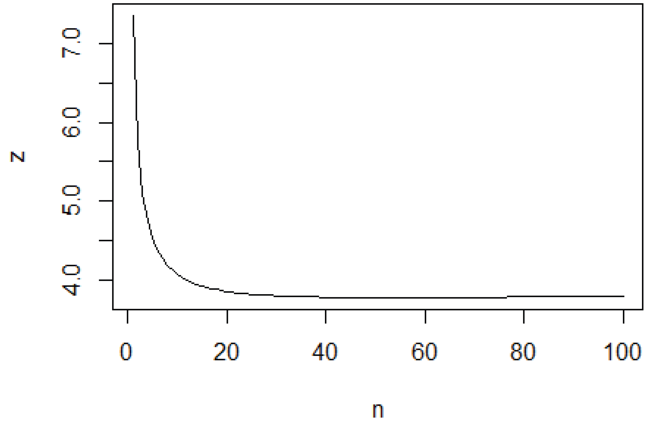
Figure 10 plots the z value needed for very strong evidence from a test against an alternative model with a medium effect size .
Figure 10.
Test against an alternative model with a medium effect size.
7. Conclusions
Let us end our paper by thinking of how a test statistic and p-value are interpreted when teaching and learning statistics. It would be typical for the p-value to simply be compared to some type I error level, with a decision of reject or fail to reject to follow. But our discussion in this paper demonstrates how there is so much more detail to consider for even a simple example. Our paper discusses further questions for an analyst to pursue. We looked at issues involving how sample size determination, stopping rules, multiple hypotheses, and effect sizes influence the quantification of statistical evidence.
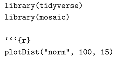
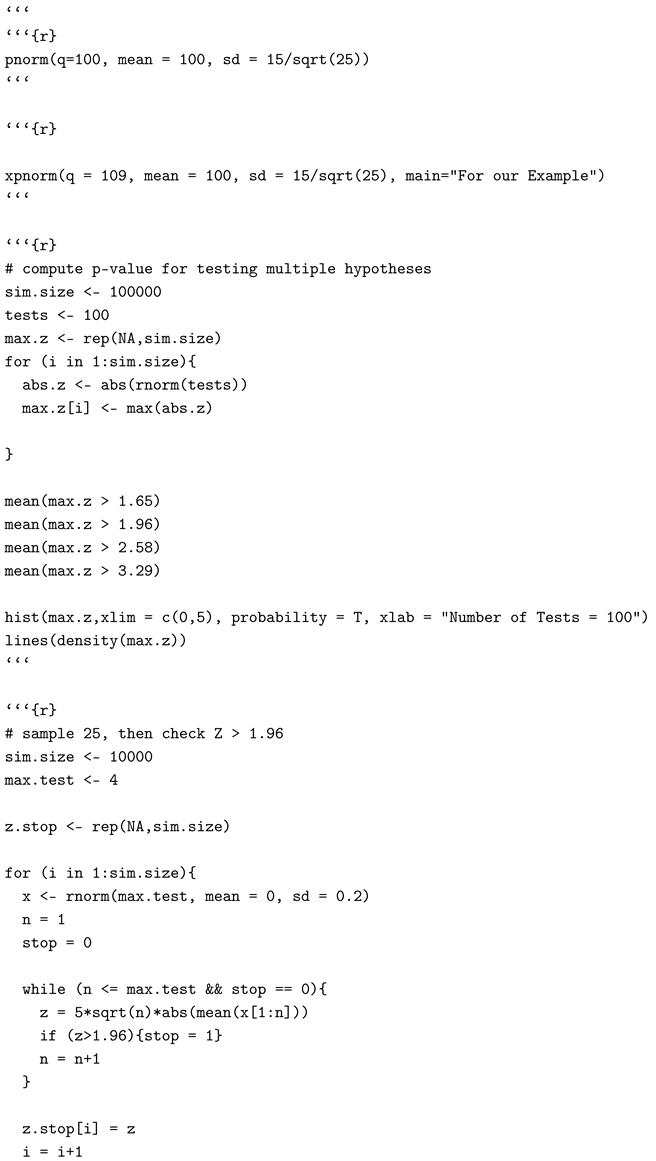
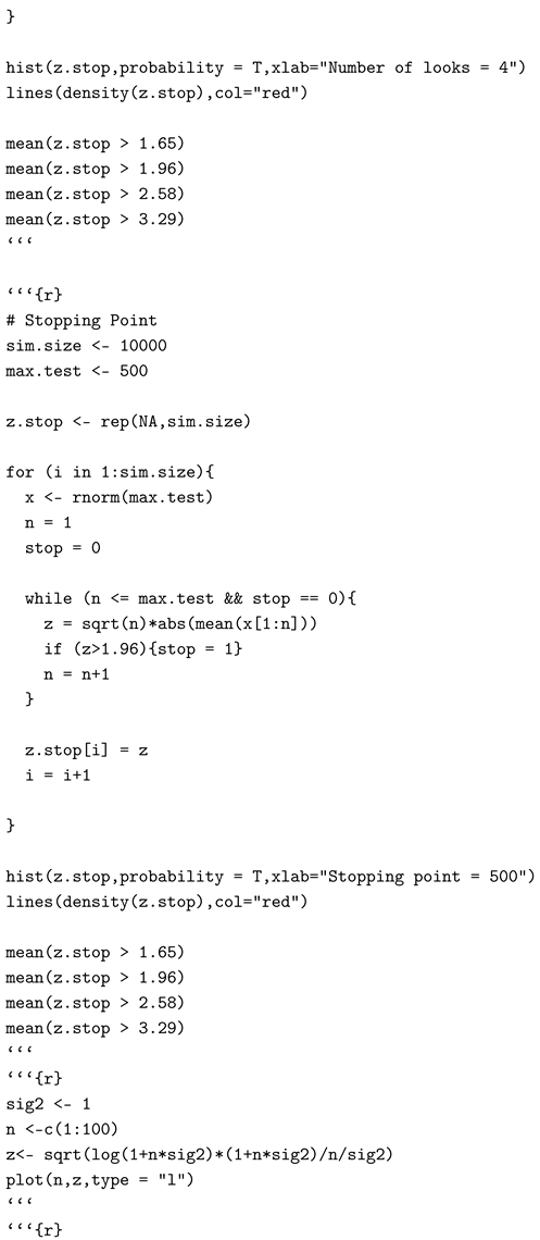
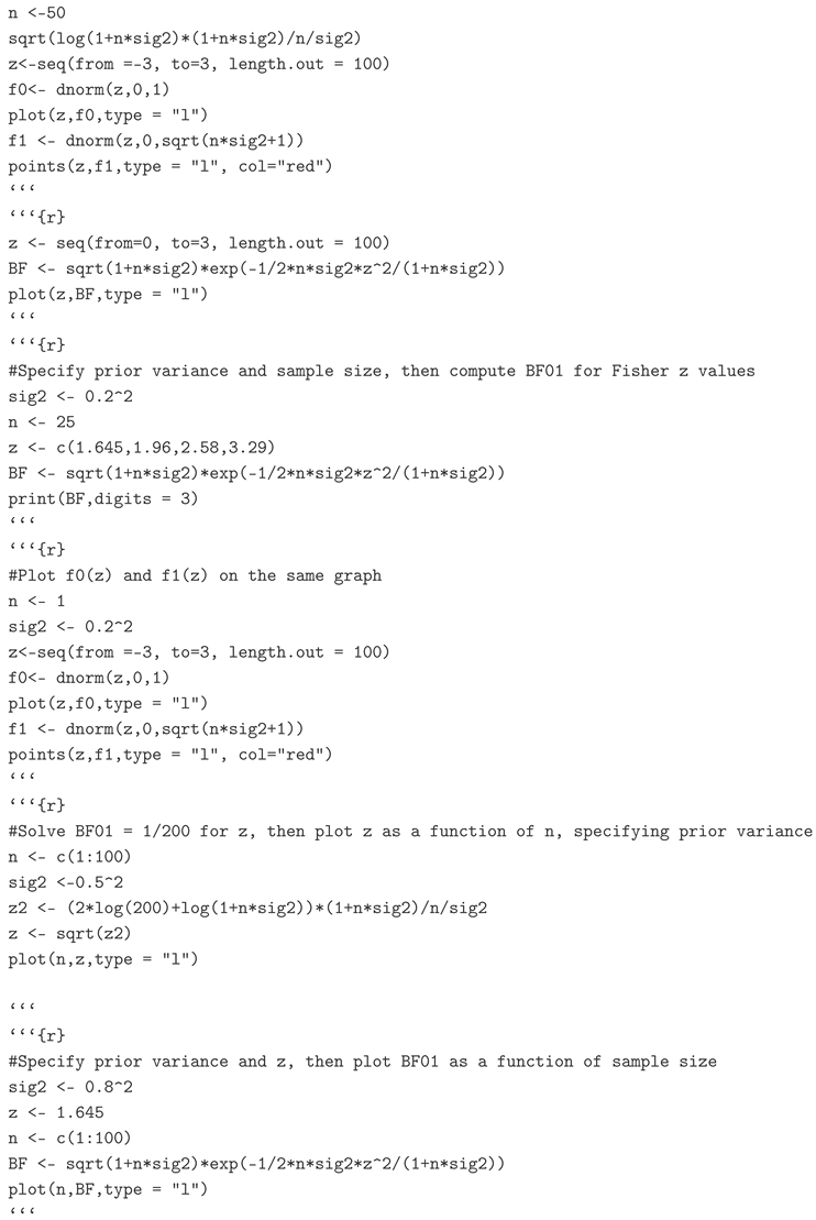
Simulations were done in R. See [7]. The relevant R code is shown below.
Author Contributions
Conceptualization, P.A.Q., A.A.N.; methodology, P.A.Q., A.A.N.; writing-original draft preparation, P.A.Q. All authors have read and agreed to the published version of the manuscript.
Funding
This research received no external funding.
Acknowledgments
The authors thank the editors and referees for their work.
Conflicts of Interest
This article is based on research previously presented in the author’s master’s thesis, "Quantifying Statistical Evidence: P-Values, the Likelihood Principle, and Bayes Factors" (Quaye, 2021). The manuscript has been condensed and reformatted for journal publication.
References
- James O Berger and Robert L Wolpert. The Likelihood Principle. IMS, 1988.
- Bradley Efron, Alan Gous, RE Kass, GS Datta, and P Lahiri. Scales of evidence for model selection: Fisher versus Jeffreys. Lecture Notes-Monograph Series, pages 208–256, 2001.
- Robert E Kass and Adrian E Raftery. Bayes factors. Journal of the American Statistical Association, 90(430):773–795, 1995. [CrossRef]
- Danielle Navarro. Bayesian Hypothesis Tests. LibreTexts in Statistics, 2020. [CrossRef]
- Andrew A Neath. A note on the connection between likelihood inference, Bayes factors, and p-values. Open Access Library Journal, 4(1):1–11, 2017.
- Yudi Pawitan. In All Likelihood: Statistical Modelling and Inference using Likelihood. Oxford University Press, 2001.
- R Core Team. R: A Language and Environment for Statistical Computing; R Foundation for Statistical Computing: Vienna, Austria, 2024.
- Agresti, A. (2013) Categorical Data Analysis. Wiley, Hoboken, NJ.
- Hubbard, R. and Bayarri, M. (2003) p-Values Are Not Error Probabilities. Institute of Statistics and Decision Sciences, Working Paper No. 03-26.
- Sellke, T., Bayarri, M. and Berger, J. (2001) Calibration of p-Values for Testing Precise Null Hypotheses. The American Statistician, 55, 62-71. [CrossRef]
- Sellke, T., Bayarri, M. and Berger, J. (2001) Calibration of p-Values for Testing Precise Null Hypotheses. The American Statistician, 55, 62-71. [CrossRef]
- Quaye, P.A. Quantifying Statistical Evidence: P-Values, the Likelihood Principle, and Bayes Factors. Master’s Thesis, Southern Illinois University, Edwardsville, IL, USA, 2021. Available online:https://www.proquest.com/docview/2544174673.
Figure 3.
Predictive distribution for multiple testing.
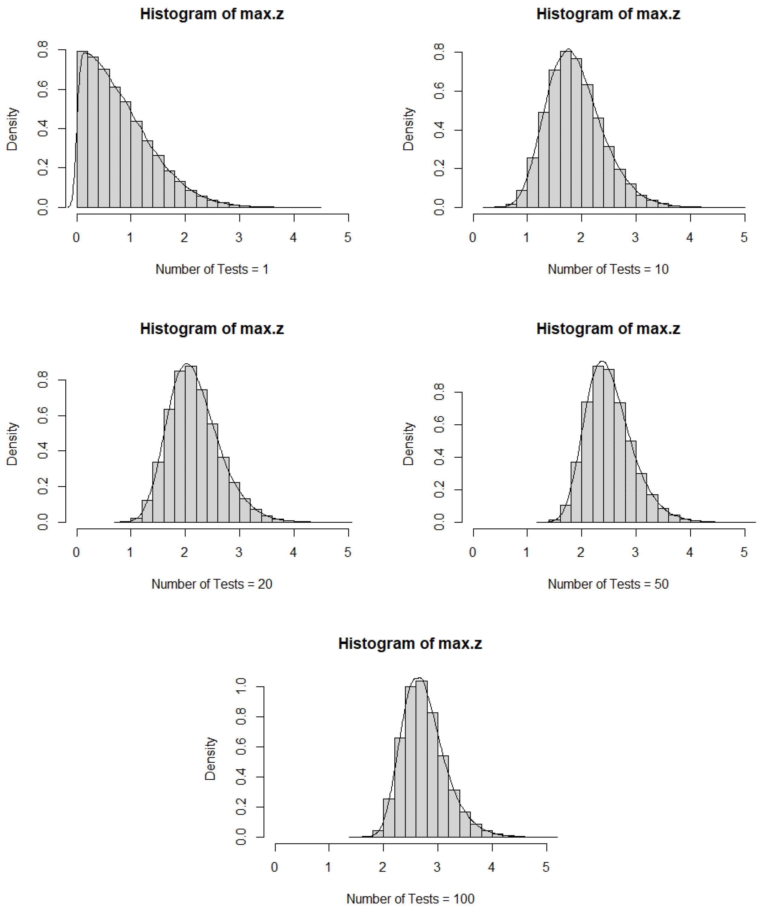
Figure 4.
Predictive distribution on the observed changes with respect to the sample size.
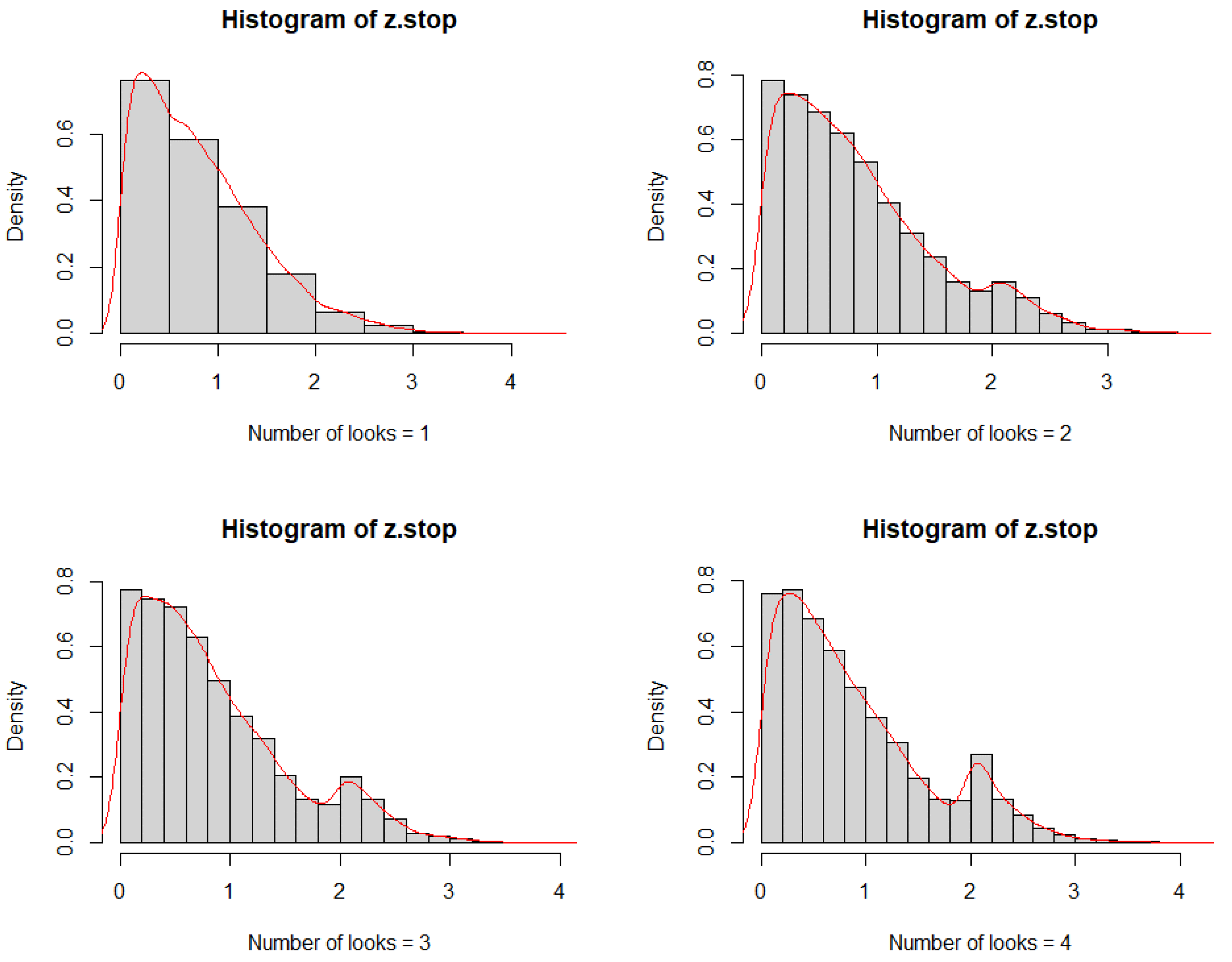
Figure 5.
Predictive distributions under this sampling scheme.
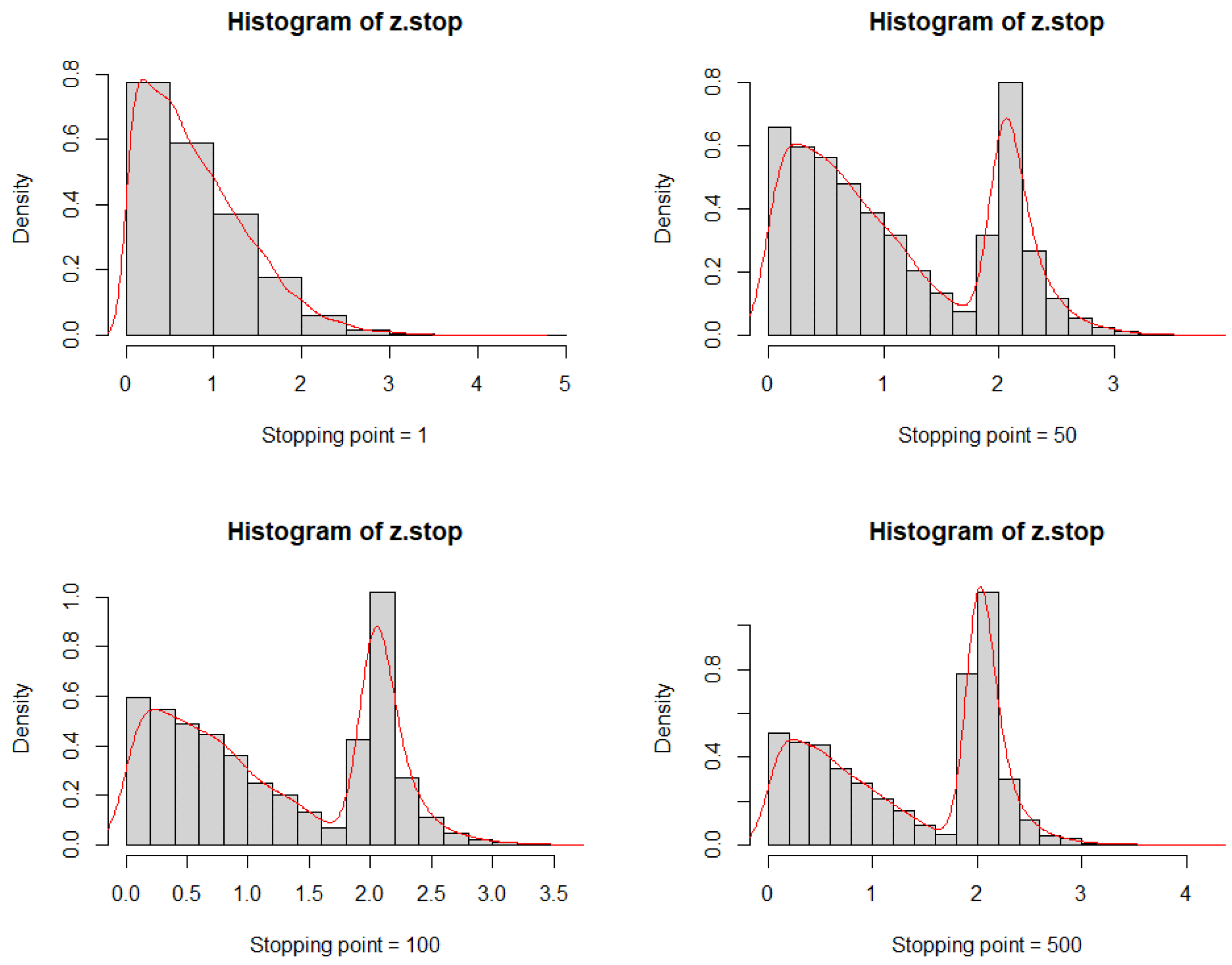
Figure 6.
Threshold separating support between the competing models, as a function of the sample size n.
Figure 6.
Threshold separating support between the competing models, as a function of the sample size n.
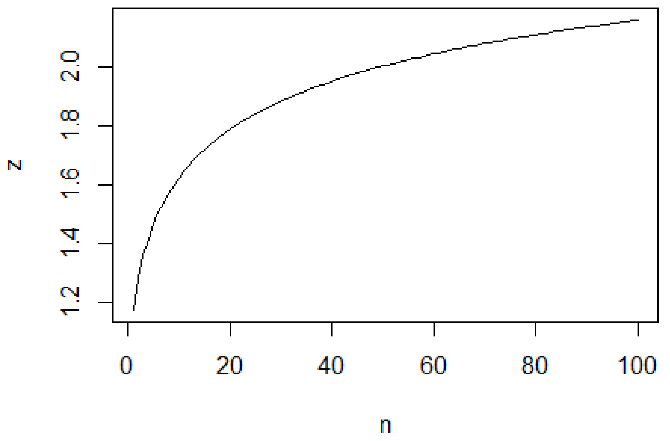
Figure 7.
Predictive densities for both models.
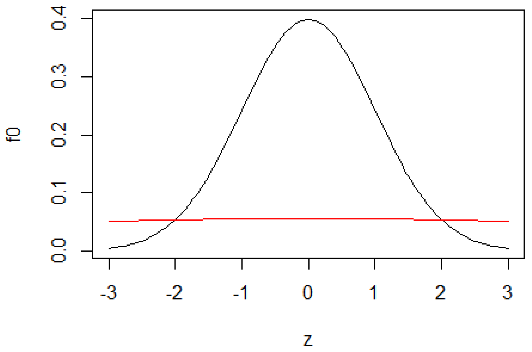
Figure 8.
Bayes factor as a function of z.
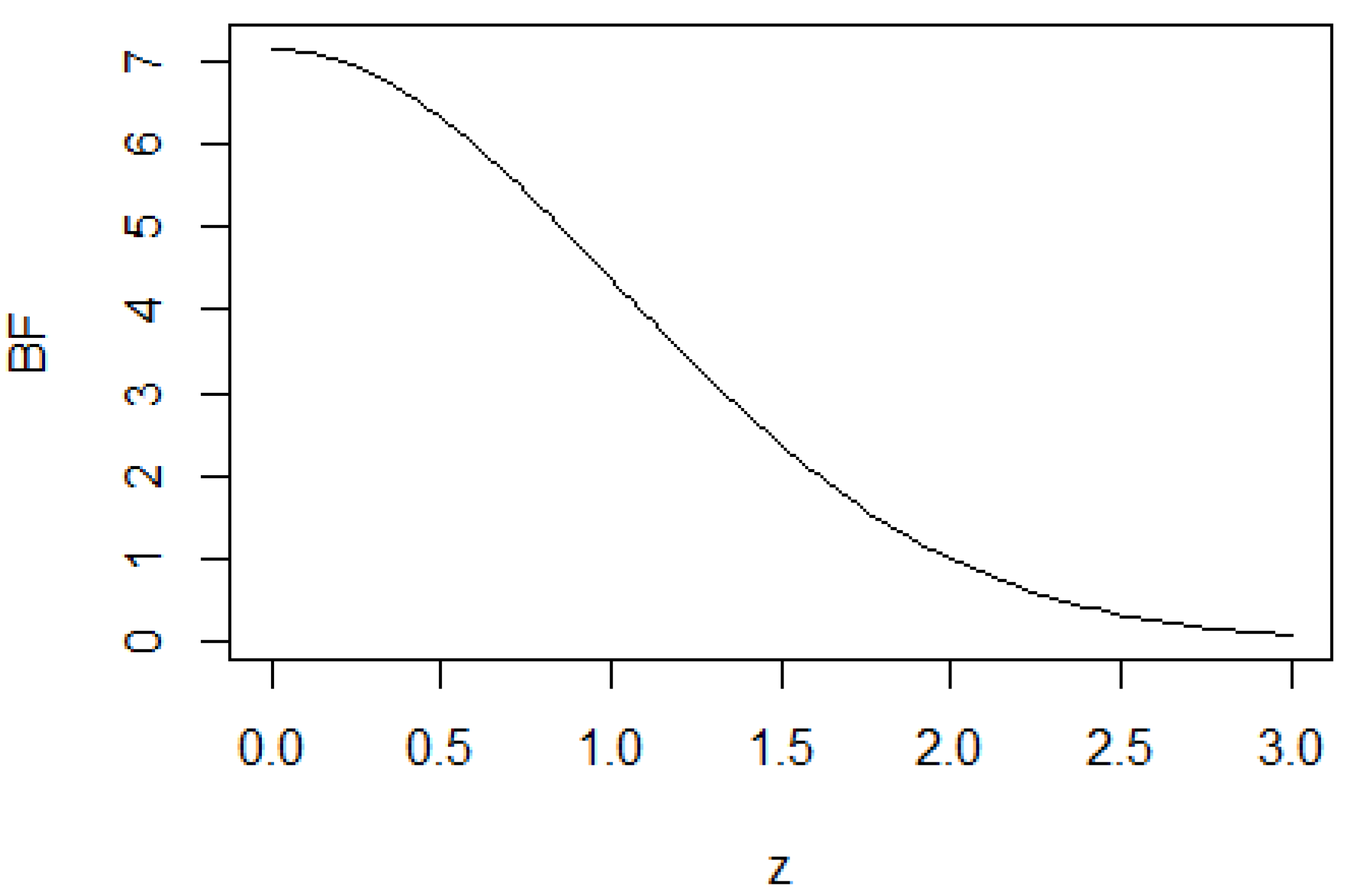
Figure 9.
Predictive Density.
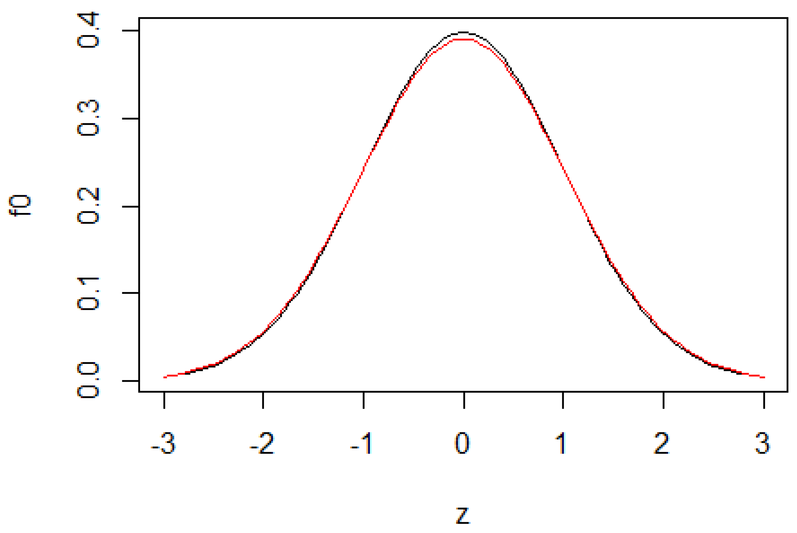
Table 1.
P-value scale for quantifying evidence.
| p | evidence against Hypothesis |
| 0.10 | borderline |
| 0.05 | moderate |
| 0.025 | substantial |
| 0.01 | strong |
| 0.001 | overwhelming |
Table 2.
LR scale of evidence.
| evidence against | |
| 0.258 | borderline |
| 0.146 | moderate |
| 0.067 | strong |
| 0.036 | overwhelming |
Table 3.
Number of tests.
| 1 | 10 | 20 | 50 | 100 | |
| 0.10 | 0.65 | 0.87 | 0.99 | 0.999 | |
| 0.05 | 0.40 | 0.64 | 0.92 | 0.995 | |
| 0.010 | 0.1 | 0.18 | 0.39 | 0.63 | |
| 0.001 | 0.01 | 0.02 | 0.05 | 0.10 |
Table 4.
Number of "looks".
| 1 | 2 | 3 | 4 | |
| 0.10 | 0.1224 | 0.1446 | 0.1635 | |
| 0.05 | 0.0828 | 0.1075 | 0.1339 | |
| 0.010 | 0.0156 | 0.0145 | 0.0182 | |
| 0.001 | 0.0021 | 0.0016 | 0.0014 |
Table 5.
Number of maximum sample size.
| z.stop | 1 | 50 | 100 | 500 |
| 0.10 | 0.3367 | 0.387 | 0.5009 | |
| 0.05 | 0.3208 | 0.3749 | 0.4922 | |
| 0.010 | 0.0214 | 0.019 | 0.0195 | |
| 0.001 | 0.0019 | 0.0012 | 0.0000 |
Table 7.
For .
| 1 | 25 | 50 | 100 | |
| 0.968 | 0.7190 | 0.7038 | 0.7575 | |
| 0.947 | 0.5413 | 0.4813 | 0.4810 | |
| 0.897 | 0.2678* | 0.1883* | 0.1560* | |
| 0.829 | 0.0945* | 0.0469** | 0.0295** |
Table 8.
For .
| 1 | 25 | 50 | 100 | |
| 0.853 | 0.8387 | 1.05 | 1.39 | |
| 0.761 | 0.5141 | 0.6205 | 0.804 | |
| 0.575 | 0.1528* | 0.1686* | 0.208* | |
| 0.379 | 0.0253** | 0.0245** | 0.028** |
Table 9.
For .
| 1 | 25 | 50 | 100 | |
| 0.755 | 1.1539 | 1.55 | 2.13 | |
| 0.605 | 0.6762 | 0.892 | 1.22 | |
| 0.349 | 0.1798* | 0.2278* | 0.3043 | |
| 0.155* | 0.0253** | 0.0302** | 0.0391* |
Disclaimer/Publisher’s Note: The statements, opinions and data contained in all publications are solely those of the individual author(s) and contributor(s) and not of MDPI and/or the editor(s). MDPI and/or the editor(s) disclaim responsibility for any injury to people or property resulting from any ideas, methods, instructions or products referred to in the content. |
© 2026 by the authors. Licensee MDPI, Basel, Switzerland. This article is an open access article distributed under the terms and conditions of the Creative Commons Attribution (CC BY) license (http://creativecommons.org/licenses/by/4.0/).
Copyright: This open access article is published under a Creative Commons CC BY 4.0 license, which permit the free download, distribution, and reuse, provided that the author and preprint are cited in any reuse.


