

Submitted:
28 June 2026
Posted:
30 June 2026
You are already at the latest version
Abstract
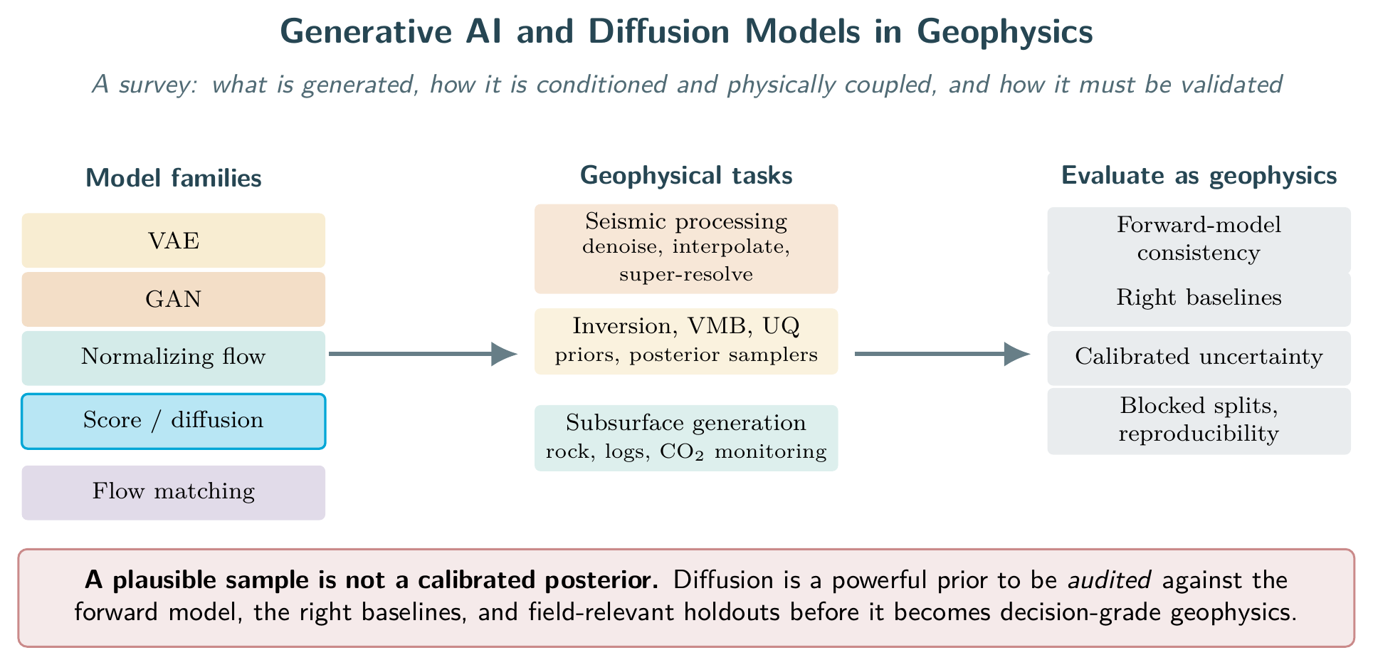
Generative modeling has become a practical prior family in geophysics, with score-based and diffusion models now used for seismic processing, inversion, subsurface monitoring, digital rock physics, well-log synthesis, and benchmark-driven reproducibility. Diffusion is best read as a restoration and posterior-sampling prior whose value depends on forward-model consistency, benchmark design, baseline coverage, and explicit uncertainty diagnostics rather than visual plausibility alone. The taxonomy links generated objects, model families, conditioning interfaces, physical coupling, and validation burden. Current evidence is strongest for seismic restoration and controlled posterior-sampling studies, and weakest for calibrated uncertainty in field-scale decisions. Scope is bounded to exploration and reservoir geophysics; ground-motion synthesis and electromagnetic, magnetotelluric, and potential-field methods are out of scope.
Keywords:
generative AI
; diffusion models
; score-based generative models
; geophysics
; seismic processing
; full-waveform inversion
; uncertainty quantification
; digital rock physics
; subsurface monitoring
; benchmarks and reproducibility
1. Introduction and Contributions
1.1. Positioning and Scope
Generative modeling is no longer a peripheral tool for geophysical machine learning. It is becoming a way to encode geological priors, sample plausible subsurface states, regularize ill-posed inverse problems, and synthesize training distributions when labeled field data are scarce. This survey is therefore organized around a specific question: how do modern generative models, especially diffusion and score-based models, change the design, validation, and failure modes of geophysical workflows? The answer is different from a generic computer-vision diffusion survey and also different from a broad machine-learning overview for geoscience. Geophysical tasks are constrained by wave propagation, acquisition geometry, rock-physics plausibility, nonunique inverse maps, and downstream decisions under uncertainty.
Prior surveys establish the need for this narrower treatment. Broad reviews of machine learning in solid-Earth science and geophysics describe the transition from feature engineering to data-driven discovery, seismic interpretation, inversion, and monitoring [1,2,3]. Seismology and seismic-exploration surveys document the rapid growth of deep neural networks for phase picking, event characterization, imaging, and exploration workflows [4,5]. In parallel, generative-model and diffusion-model surveys compare model families and image-domain applications at the machine-learning level [6,7,8]. A recent geoscience review broadens the discussion to generative AI and large language models [9]. These works are necessary context, but they do not give a diffusion-centered map of geophysical use cases, conditioning mechanisms, physics coupling, and reproducibility obligations.
We draw that map by treating generative adversarial networks (GANs), variational autoencoders (VAEs), and normalizing flows as important pre-diffusion baselines and priors, while using denoising diffusion and score-based generative modeling as the main organizing thread [10,11]. This choice reflects both methodological momentum and geophysical fit: iterative denoising and score estimation align naturally with noisy measurements, posterior sampling, and data-consistency corrections in inverse problems [12]. We also cover latent diffusion when the main challenge is scale or representation learning rather than pixel- or sample-level synthesis [13].
The scope is intentionally bounded. Included are generative models for seismic processing, interpolation, denoising, deblending, super-resolution, velocity and property-model generation, full-waveform inversion, uncertainty quantification, digital rock physics, well-log synthesis or imputation, and time-lapse or monitoring settings. We include representative earlier GAN-based geophysical priors because they explain the continuity from learned geological latent spaces to diffusion priors in inverse problems [14,15]. We exclude general remote-sensing image generation, climate or weather generation, and large-language-model papers unless they directly affect geophysical data, modeling, benchmarking, or scientific workflow design. Classical geostatistical simulation is treated as background rather than surveyed exhaustively. We focus on seismic, reservoir, and subsurface-characterization workflows. Earthquake and engineering seismology with ground-motion synthesis, ground-penetrating radar, electromagnetic and magnetotelluric methods, and potential-field methods are outside this survey and warrant separate treatment.
1.2. Taxonomy
The taxonomy in Table 1 separates five questions that are often mixed together: what object is generated, what generative family is used, how the model is conditioned, how it is coupled to the governing physics, and what form of geophysical validation is required. This separation matters because two papers can both be called “diffusion for seismic” while solving quite different problems: one may denoise shot gathers in data space [16], another may generate controllable velocity models in model space [17], and a third may use a generic diffusion posterior sampler as a prior inside an inverse problem [12].
The application sections follow this taxonomy rather than a simple list of architectures. Seismic-processing methods are grouped by whether generation acts as restoration, interpolation, or acquisition compensation. Inversion and uncertainty methods are grouped by whether the generator is a low-dimensional geological prior, an amortized inverse map, or a posterior sampler. Subsurface generation is grouped by the object scale, from pore images and logs to reservoir-scale property fields. Benchmark and reproducibility coverage then cuts across all application areas, because the evidence standard changes when a method moves from synthetic benchmarks to field data, from 2-D to 3-D, or from single-realization reconstruction to calibrated uncertainty. Open benchmarks such as OpenFWI make this distinction concrete by coupling seismic data, subsurface models, baselines, and generalization tests in a form that exposes both promise and limitations [18].
1.3. Contributions
We position generative geophysics relative to prior deep-learning, seismology, diffusion-model, and generative-AI surveys, locating the missing geophysics-specific layer between model-family reviews and application papers. We organize that layer through a compact taxonomy (Table 1) and an explicit cross-walk (Table 2) that link application families to generated objects, model families, conditioning mechanisms, physics coupling, and validation burden, with diffusion and score-based models as the methodological spine and earlier generative approaches retained as baselines and historical context. Throughout, benchmarks, uncertainty, and reproducibility are treated as primary axes, not closing caveats, because generative samples are useful in geophysics only when they remain plausible under the governing measurements and the intended downstream decision.
2. Background: A Methods Spine for Generative Geophysics
2.1. From Latent Variables to Transport Paths
Deep generative modeling in geophysics can be organized by what is made explicit: a latent representation, a density, a discriminator, a score field, or a transport velocity (Figure 1). Variational autoencoders (VAEs) introduce probabilistic encoder and decoder networks and optimize an evidence lower bound, making them useful when a compact latent variable is desired for facies, velocity, log, or image families [19]. Generative adversarial networks (GANs) instead train an implicit generator by matching generated and observed samples through a discriminator [20]. This implicit view has been attractive in geophysical settings where visually plausible realizations are useful, but it does not by itself provide a tractable likelihood or posterior uncertainty; recent seismic inversion work therefore tends to add model, physics, or data-consistency constraints rather than use an unconstrained GAN alone [21].
Normalizing flows make the density explicit by composing invertible maps and evaluating
The appeal is exact likelihood evaluation and reversible sampling [22,23,24]. The limitation is also structural: invertibility and tractable Jacobians constrain architectures, while high-dimensional seismic cubes and multiphysics model spaces often need aggressive conditioning or block structure. Flows are best treated as the likelihood-calibrated branch of the taxonomy, not as predecessors that diffusion simply replaced.
2.2. Score and Diffusion Models
Diffusion models replace one-shot generation with a sequence of denoising or reverse-time transport steps. The early nonequilibrium thermodynamics view defines a forward noising process and learns the reverse process [25]; denoising diffusion probabilistic models (DDPMs) made this practical with a simplified denoising objective derived from a reweighted variational bound and a neural denoiser [10]. A parallel score-based line learns and samples with Langevin dynamics or the reverse stochastic differential equation [11,26]. DDIM-style samplers expose a deterministic non-Markovian path that can reduce sampling cost while preserving the same trained denoiser [27].
The geophysical relevance is not only sample quality. Seismic denoising, interpolation, reconstruction, diffraction separation, and interpretation tasks can be written as restoring missing or corrupted observations under acquisition and wave-propagation constraints. Recent seismic papers use diffusion or score-based models for denoising, interpolation, reconstruction, and guided generation [28,29,30,31,32]. The evidence so far is narrow but consistent: diffusion has become a credible restoration prior for seismic data, concentrated in processing and interpolation rather than complete end-to-end field-decision workflows.
2.3. Latent, Conditional, and Physics-Guided Diffusion
Latent diffusion moves the denoising process from pixel or trace space into an autoencoded latent space, reducing memory and allowing higher-resolution generation when the autoencoder preserves task-relevant structure [13]. This is especially relevant for 3-D seismic volumes, where direct denoising over full cubes is often limited by memory and where representation learning can separate local texture from larger structural events; a recent seismic latent-diffusion interpolation example follows this direction [33].
Conditioning is the main bridge from generic generation to geophysical inference. Classifier-free guidance shows that conditional and unconditional scores can be combined at sampling time to trade diversity for condition adherence [34]. In inverse problems, diffusion posterior sampling and related reconstruction-guided methods inject a forward model into the reverse process, using the learned prior to regularize the ill-posed update [12,35]. Geophysical variants can condition on acquisition masks, migrated images, well logs, velocity bounds, rock-physics transforms, or partial-differential-equation (PDE) residuals. Existing inversion examples already combine diffusion priors with post-stack inversion, FWI regularization, and Bayesian full-waveform sampling [36,37,38,39]. The unresolved methodological issue is calibration: a guided sampler can improve data consistency without proving that the retained sample spread is a calibrated posterior for the subsurface property of interest.
2.4. Flow Matching and Rectified Flows
Flow matching returns to a continuous-time transport view but trains a velocity field rather than a noise-prediction or score field. Given paired endpoints or a chosen probability path between noise and data, the model learns an ODE velocity whose integration maps a simple base distribution to the data distribution [40]. Rectified flow and stochastic interpolants make related design choices: choose interpolants that make paths straighter, easier to integrate, or easier to couple with simulation constraints [41,42].
For geophysics, flow matching is promising because the language of trajectories fits continuation, time-lapse monitoring, and inverse-problem homotopies. However, it remains an emerging methodological branch, not an established geophysical replacement for diffusion. The open question is whether flow-matching velocity fields can enforce acquisition geometry, PDE residuals, and hard well constraints with fewer sampling steps than diffusion while retaining uncertainty diagnostics.
Table 3 summarizes these families and their roles in a geophysical generative workflow.
3. Seismic Processing Applications
3.1. Problem Setting
Seismic processing is the most direct entry point for generative models because many production tasks can be written as conditional restoration problems. Let x denote a clean gather, image, or volume, y the observed data, and a masking, sampling, blending, bandwidth, or noise operator. Diffusion and score-based methods estimate samples from a conditional distribution rather than a single deterministic map. This is attractive for ill-posed processing, but it also creates an obligation: output uncertainty, residual spectra, moveout consistency, and downstream imaging behavior must be checked, because visually plausible events can be geologically wrong.
3.2. Denoising and Joint Restoration
Recent work shows that diffusion models are now being used for multi-dimensional seismic noise attenuation, not merely as generic image priors. Xiao et al. use diffusion models for multidimensional seismic noise attenuation and super-resolution, framing restoration as a learned reverse process rather than a direct filter [43]. Meng et al. extend this idea to stochastic, simultaneous denoising and reconstruction with score-based generative models, which is important because acquisition gaps and noise are coupled in practice [44]. Peng et al. address a practical bottleneck by proposing a fast diffusion model for seismic noise attenuation [45]. These papers support a cautious conclusion: diffusion models are credible seismic denoisers when the noise class and sampling geometry resemble training conditions. Field-ready generality still requires blind tests across crews, instruments, and processing flows.
The surrounding literature is already broad enough to justify a separate denoising subcategory. Recent papers study alternative training strategies, unsupervised diffusion denoising, generalized diffusion denoisers, diffusion restoration, and three-dimensional diffusion or Fourier-neural-operator guidance [28,46,47,48,49]. Denoising is now active diffusion literature, while anisotropic diffusion filtering remains a classical processing baseline rather than a generative model [50]. Diffraction separation and imaging form a related restoration problem, with conditional DDPM evidence now available [29].
3.3. Interpolation and Reconstruction
Interpolation is a stronger test of generative priors because the model must recover coherent events where traces are missing rather than suppress additive noise only. Wei et al. combine denoising diffusion implicit models with coherence-corrected resampling for seismic interpolation [51]. Wang et al. propose SeisFusion, a constrained diffusion model with input guidance for 3-D seismic interpolation and reconstruction [31]. Together with the joint denoising-reconstruction formulation of Meng et al. [44], these results suggest a useful taxonomy: masks and acquisition geometry should enter the sampler explicitly; coherence constraints reduce event drift; and evaluation should include f-k spectra, gather-domain residuals, and migration or inversion sensitivity, not only pixelwise peak signal-to-noise ratio (PSNR) or structural similarity (SSIM).
Additional interpolation references reinforce the same point. They include refined diffusion posterior sampling for denoising and interpolation, score-based diffusion with wavelet convolution, diffusion-based interpolation deep learning, a recent 3-D DDPM interpolation survey, and pre-diffusion GAN or conditional-GAN interpolation baselines [52,53,54,55,56,57]. Older trace interpolation and ray-tracing interpolation papers are useful only as non-generative baselines for acquisition geometry and moveout behavior [58,59].
3.4. Super-Resolution and Bandwidth Extension
Seismic super-resolution differs from photographic super-resolution because the added high frequencies affect apparent thin-bed tuning, fault continuity, and attribute interpretation. Non-diffusion deep baselines already study simultaneous seismic image super-resolution and denoising [60]. Generative variants include a CycleGAN resolution-enhancement method using pseudo-well data [61] and SeisResoDiff, a diffusion model for seismic resolution enhancement [62]. Generative models do not “recover missing bandwidth”; they learn conditional high-frequency completions. Such completions require external checks against well ties, wavelet estimates, phase behavior, and pre-stack amplitude fidelity before they should influence stratigraphic or reservoir decisions.
The super-resolution baseline space remains heterogeneous. Stabilized deep generative seismic super-resolution is directly relevant [63], whereas many generic image super-resolution GAN papers in the broader reference pool are off-domain and should not support geophysical claims without a seismic experiment.
3.5. Deblending and Source Separation
The evidence base for diffusion-specific seismic deblending is thinner than for denoising and interpolation. A representative deep-learning reference is the convolutional neural network approach of Sun et al. for deblending seismic data [64]. Diffusion could in principle treat blended data as and sample separated shot records subject to the known blending operator, but current evidence does not yet justify presenting diffusion deblending as established. Deblending is better read as a promising but under-benchmarked frontier, with strict requirements for crosstalk residuals, weak-event preservation, and tests on realistic simultaneous-source schedules.
The baseline literature for this frontier is not thin: deblending papers cover physics-augmented learning, shot-domain deep learning, self-supervised blind-trace networks, inversion-based neural deblending, self-supervised blind-spot denoisers, and time-lapse settings [65,66,67,68,69,70]. Sparse inversion remains a necessary classical comparator [71]. A diffusion paper that omits these comparators should be described as exploratory, not conclusive.
3.6. Ground-Roll Attenuation
Ground-roll attenuation is a useful stress test because surface waves overlap reflection signal in time, offset, and frequency. Kaur et al. demonstrated ground-roll attenuation using a generative adversarial network in EAGE proceedings [72] and later studied seismic ground-roll noise attenuation using deep learning in Geophysical Prospecting [73]. These are not diffusion papers, but they are important generative/deep baselines for the processing taxonomy. The main limitation is interpretational: aggressive attenuation can erase low-frequency signal or distort shallow reflection amplitudes. What matters is the residual gather and signal leakage, not a cleaner-looking section.
3.7. Data Augmentation and Training-Set Design
Treat generative augmentation as a controlled experimental device, not a substitute for field diversity. Li et al. use conditional GANs for seismic data augmentation [74]. This supports augmentation for class balancing, robustness tests, and pretraining when labels or rare events are scarce. However, augmentation can leak model bias into downstream evaluation if synthetic and real examples share the same generator artifacts. The minimum standard is a real-only held-out test set, ablations that separate synthetic pretraining from real-data fine-tuning, and documented acquisition, geology, and preprocessing differences between generated and target data.
Earlier GAN-based processing papers are useful historical baselines for this discussion, including land-seismic noise removal, random-noise suppression, general seismic processing with GANs, and low-cost sensor augmentation [75,76,77,78]. They should be cited as baselines and design precedents, not as evidence that diffusion models inherit field robustness automatically. Table 4 summarizes the processing use cases surveyed in this section.
3.8. Cross-Cutting Evaluation Requirements
Across these applications, diffusion and other generative models should be evaluated as geophysical processors rather than image enhancers. At minimum, papers should disclose training data provenance, masking or blending operators, normalization and phase conventions, compute cost, and failure cases. Metrics should combine sample-domain errors with spectral diagnostics, coherency or slope consistency, residual leakage, and task-level effects on migration, attribute extraction, inversion, or interpretation. Where stochastic sampling is used, reporting multiple posterior samples or credible intervals is more informative than a single best-looking section.
4. Inversion, Velocity-Model Building, and Uncertainty Quantification
Among generative-geophysics applications, seismic inversion imposes the heaviest validation burden: the forward map is expensive, nonlinear, and often only weakly identifies the subsurface parameters of interest. In acoustic or elastic full-waveform inversion (FWI), one seeks a model m such that simulated data match observed shot gathers d, typically by minimizing a data misfit plus a regularization term weighted by . The classical FWI literature already framed this as a least-squares, local-optimization inverse problem [79,80], but practical workflows still face cycle skipping, acquisition gaps, source and noise uncertainty, and strong non-uniqueness. Multiscale continuation is a durable mitigation strategy [81]; it does not by itself produce calibrated posterior uncertainty. Modern diffusion and score-based methods should therefore be evaluated not as generic image priors, but as ways to encode geological regularity while remaining compatible with the wave-equation likelihood and the Bayesian inverse-problem view [82].
Additional FWI and velocity-model-building baselines include direct waveform inversion, acoustic and robust FWI variants, full-model wavenumber inversion, reflection FWI, damped-frequency-domain FWI, joint traveltime and envelope inversion, and wave-equation reflection traveltime tomography [83,84,85,86,87,88,89,90,91]. These methods define the non-generative baseline that diffusion regularizers must improve on or complement.
4.1. From Learned Velocity Builders to Inverse-Problem Samplers
The current literature separates into three related, but distinct, roles for generative models. First, data-driven velocity-model builders learn a direct map from seismic observations to velocity images, often using synthetic families such as OpenFWI [18]. These models can be useful for warm starts, rapid screening, or amortized uncertainty summaries, as in machine-learning velocity-model-building work that explicitly reports uncertainty [92]. Their limitation is that supervised synthetic-to-field transfer and posterior calibration remain separate questions.
Generalization studies on OpenFWI-like settings show why this matters: a network can perform well on one structural family yet degrade under geological or acquisition shift [93]. Classical Marmousi velocity-model-building studies remain useful stress tests because they expose complex structures that simple pixel losses can hide [94,95].
A second role places diffusion models as learned regularizers inside an FWI loop. Wang et al. use a generative diffusion prior to steer acoustic FWI toward plausible models [96]. Taufik et al. extend this idea to multi-parameter elastic FWI, where the coupling among elastic parameters makes learned regularization especially attractive [97]. Conditional variants introduce explicit geological or well-log information into the prior [98], and recent preprints investigate using the diffusion prior itself as a direct regularization term [99]. These approaches are closest to production FWI: they preserve a deterministic optimization backbone, but the reported uncertainty is usually indirect unless the method also samples or ensembles solutions.
Recent extensions make this role a fast-moving target. They include learned diffusion regularization for FWI, efficient 3-D velocity-model building with reconstruction-guided conditional diffusion, and broader surveys of generative models for seismic processing and velocity-model building [100,101,102]. They show clear momentum, though much of it still sits in preprints and expanded abstracts rather than peer-reviewed articles.
The third role uses score-based models as posterior samplers. The methodological spine comes from denoising diffusion and score-SDE models [10,11]; inverse-problem solvers then combine a learned score with a data-consistency or likelihood gradient [12,103,104]. In geophysics, measurement-guided diffusion explicitly adapts this recipe to inverse problems with physical forward operators [105]. For FWI, DiffusionInv and reconstruction-guided diffusion sampling are the most direct posterior-sampling examples: they use diffusion-generated priors while forcing samples back toward seismic data consistency [39,106]. The main promise is not just sharper velocity images; it is access to multiple plausible models drawn from the posterior for the same data. Table 5 contrasts these three roles.
4.2. Uncertainty Quantification and Posterior Diagnostics
The key distinction is whether a method returns uncertainty because it samples a posterior, ensembles deterministic reconstructions, or predicts a surrogate variance. Normalizing-flow tomography and FWI work provides a useful baseline because it makes the density transformation explicit [107,108]. Amortized variational inference with physics-based latent correction is another relevant baseline: it starts from a learned inverse map but corrects the latent distribution using the physics likelihood [109]. Ensemble and importance sampling schemes for seismic inversion similarly emphasize posterior diagnostics rather than only image quality [110,111].
Beyond seismic FWI, diffusion-based uncertainty quantification is already being tested in other geophysical Earth-system calibration settings [112]; such papers are useful for UQ methodology transfer but should not be used as direct evidence for seismic inversion performance.
Diffusion posterior samplers inherit both strengths and hazards from these baselines. They can represent multimodality, preserve sharp geological features, and condition on sparse prior information. However, an attractive sample set is not enough. A geophysical UQ claim should state the forward operator, noise model, prior and conditioning data, and likelihood scale, and report diagnostics such as data-residual coverage, posterior predictive checks, and sensitivity to the starting model and acquisition geometry. In FWI specifically, the cost of many score steps times many wave-equation solves can dominate the workflow; papers that amortize, surrogate, or partially linearize this coupling should report the approximation and where it fails.
4.3. Practical Reading of the Evidence
The evidence is strongest for diffusion as a learned geological regularizer and as a research-grade posterior sampler on controlled seismic examples. It is weaker for field-scale calibrated UQ, where source uncertainty, anisotropy, elastic parameter cross-talk, bandwidth limits, and modeling error can dominate the nominal posterior. The most credible near-term workflows are hybrid: use diffusion or score models to propose geologically plausible ensembles, then retain wave-equation data consistency and Bayesian diagnostics before turning samples into decisions. Claims of “uncertainty” should therefore be read narrowly unless the paper demonstrates posterior calibration against held out physics, wells, horizons, or repeated acquisitions.
5. Digital Rock, Well Logs, and Subsurface Monitoring
5.1. Application Scope
Subsurface generation sits closer to rock physics and reservoir decision-making than generic image synthesis. The useful question is not whether a model can produce plausible-looking pores, facies, logs, or plumes, but whether generated samples preserve the conditioning data, transport-relevant geometry, and uncertainty needed by a downstream simulator or interpreter. The sources reviewed here separate four uses: digital-rock and pore-scale synthesis, reservoir-facies priors, well-log synthesis or imputation, and time-lapse monitoring of storage reservoirs.
5.2. Digital Rock and Porous Media
GAN-based digital rock papers established the basic promise of learned generative priors for three-dimensional pore geometry. Mosser et al. trained a GAN to reconstruct 3-D porous media from image data [113]; the same group then used GANs for stochastic reconstruction of oolitic limestone [114]. These papers moved digital-rock reconstruction away from hand-designed statistical matching alone, but they also make the evaluation problem sharper: a pore image that matches local texture can still fail on connectedness, percolation, capillary behavior, or simulated permeability. More recent diffusion work extends the same objective to multiphase pore-scale images and controlled latent reconstruction [115,116]. On current evidence, diffusion models are becoming a competitive pore-image prior, but they have not solved digital rock physics. Matching texture is the easy part; the harder tests are morphological statistics, phase connectivity, simulated flow, and rock types held out from training.
5.3. Reservoir Facies and Geological Priors
At reservoir scale, generative models are used less as image enhancers and more as parameterizations of geological uncertainty. Laloy et al. used a spatial GAN for training-image-based geostatistical inversion [14], while Zhang et al. generated 3-D reservoir facies models by learning sedimentary architecture with GANs [117]. These studies are important because they tie generation to inversion or geological realism rather than unconditional sampling. The limitation is equally important: a generator compresses the training-image prior. If the prior lacks fault styles, channel geometries, diagenetic overprints, or depositional regimes present in the target field, the posterior samples may look coherent while excluding valid geology. Reservoir generators should therefore report conditioning-data honor, prior coverage, history-match sensitivity, and ensemble diversity instead of only visual examples.
5.4. Well Logs, Borehole Images, and Missing Curves
Well-log generation is a distinct sequence problem because depth trends, stratigraphic breaks, tool physics, and cross-log constraints matter. A recent sequence GAN study targets both generation and imputation of well-log data [118], and Meng et al. formulate missing-log imputation with conditional denoising diffusion probabilistic models [119]. A related borehole-imaging direction uses GAN translation from microresistivity image logs to synthetic carbonate core images with Dunham texture labels [120]. These papers justify including well-log synthesis in the generative-geophysics taxonomy, but they also expose risks that are easy to miss in aggregate metrics. Imputed logs should be evaluated on blind wells, interval-level facies changes, petrophysical cross-plots, and downstream saturation, porosity, or rock-typing decisions. Synthetic borehole images need independent sedimentological or core-based validation before they are treated as substitutes for core observations.
5.5. CO2 Storage and Time-Lapse Monitoring
Generative modeling for CO2 storage is best viewed as a monitoring and forecasting surrogate under hard physical constraints. Time-lapse (4-D) seismic is the classical monitoring frame for CO2 sequestration [121]. Within that frame, Zhong et al. used a conditional deep convolutional GAN to predict CO2 plume migration in heterogeneous formations [122]. Later work connects generative surrogates more directly to seismic observations: Yu et al. used a 3-D conditional Wasserstein GAN (cWGAN) to reconstruct Sleipner crosslines [123], a DDPM predicts CO2 plume evolution from seismic shot gathers [124], and diffusion-based multiphysics monitoring forecasts subsurface CO2 states [125]. Deep full-waveform inversion for CO2 saturation and uncertainty is not itself a generative model, but it provides a useful monitoring baseline for uncertainty-aware claims [126]. This literature is active but still validation-limited: it supports rapid ensembles, data assimilation, and scenario screening, but does not replace mass-balance checks, pressure constraints, plume-volume consistency, and blind time-lapse validation.
Table 6 groups the four application clusters.
5.6. Cross-Cutting Limitations
Across these subsurface topics, the central failure mode is plausible synthesis that is not decision-faithful. Generative models can provide compact priors, missing-data imputers, and fast scenario ensembles when their conditioning variables and physics checks are explicit. They should not be described as producing measurements. Beyond the cluster-specific checks above, the one report that carries across all four uses is provenance: where the training data came from, how it was preprocessed, and which conditioning variables fix what a sample is allowed to honor.
6. Datasets, Benchmarks, Metrics, and Reproducibility
Benchmarks for diffusion and score-based geophysical modeling should be treated as measurement instruments, not just as convenient image corpora. A credible benchmark specifies the acquisition geometry, forward operator, preprocessing, train/validation/test split, leakage controls, physical units, and evaluation protocol. This is especially important for generative models because visually plausible samples can be unphysical, can memorize local structures, or can score well under pixel metrics while failing the downstream geophysical decision.
6.1. Dataset Families and Benchmark Roles
Table 7 lists representative datasets and their benchmark roles. OpenFWI is the cleanest starting point for benchmarked full-waveform inversion because it links the learning target to an explicit forward-modeling task and reports baselines across multiple structural families [18,127]. Its public benchmark tables use MAE, RMSE, and SSIM, which are useful for model-level comparability but should not be read as a complete physics validation suite [128,129]. A diffusion paper using OpenFWI should therefore report both within-family performance (e.g., FlatVel-A to FlatVel-A) and transfer tests across harder families (e.g., flat to faulted or Kimberlina-like structures). Otherwise, a method may look strong because it has learned the benchmark generator rather than the inverse problem.
Marmousi remains valuable because it is a compact, recognizable failure case for velocity-model building: strong lateral velocity variation, complex reflector geometry, and sharp contrasts make it hard to hide instability behind mean pixel error [130]. It should be used as a controlled stress-test rather than as a leaderboard by itself. Authors should state the exact Marmousi version, grid spacing, crop, source-receiver geometry, frequency band, boundary conditions, and whether labels are true velocity, smoothed velocity, migrated images, impedance, or another derived quantity.
SEG/EAGE-style salt examples fill a different role: they test whether a method can handle strong velocity contrast and illumination gaps around salt bodies. The original SEG/EAGE salt family has appeared in many smoothed and simulated forms; a paper should cite the actual variant and data-generation recipe rather than only naming the benchmark [131,132]. For diffusion methods, this is where sample diversity must be judged against physics: multiple posterior samples are useful only if they explain the observed data and preserve geologically plausible salt boundaries.
The F3 Netherlands offshore survey is essential because synthetic performance does not guarantee field robustness. The TerraNubis F3 Demo 2023 project documents a public OpendTect package with 2-D and 3-D seismic data, acoustic impedance, wells, horizons, and derived attribute volumes [133]. That richness is also a leakage hazard. If a model predicts faults, horizons, impedance, facies, or well-log-derived attributes from F3 seismic, the split must be spatially blocked at survey scale, not randomly sliced. Adjacent slices share coherent reflectors; random inline/crossline crops can make train and test examples nearly duplicate. Derived products should be classified as either inputs, labels, baselines, or forbidden side information before training begins.
6.2. Metrics for Generative Geophysics
Table 8 groups complementary metric classes for generative geophysics. For reconstruction tasks, OpenFWI-style MAE/RMSE/SSIM tables are a practical minimum [128,129]. For diffusion models, the minimum is not enough. A generative benchmark should also evaluate distributional realism and data consistency. FID can be useful as a warning signal for sample collapse or distribution shift [134], but a generic Inception embedding is not a seismic representation. A better geophysical protocol reports spectral statistics, reflector continuity, attribute histograms, and forward-modeled data residuals beside any learned embedding score.
Uncertainty metrics need particular care. Posterior sample variance should not be advertised as calibrated uncertainty unless credible intervals are checked against withheld ground truth or repeated synthetic trials. For field data, where true subsurface labels are unavailable, authors should report consistency with observed gathers, well ties where available, and sensitivity to plausible forward-model, noise, and preprocessing choices.
6.3. Leakage, Splits, and Reporting Standards
Leakage is the most likely way to overstate progress in geophysical ML benchmarks. The general ML literature documents leakage as a reproducibility failure mode [135]; in geophysics it often appears through spatial correlation, reused simulated generators, derivative labels, and hidden preprocessing. The following controls should be mandatory:
- Spatial blocking: field surveys should be split by contiguous survey regions, wells, horizons, or acquisition lines as appropriate; random patch splits are insufficient for coherent 3-D seismic.
- Generator blocking: synthetic data should include held-out model families, geological styles, frequency bands, source signatures, and noise levels, not only held-out random seeds.
- Derivative-product separation: attributes, horizons, wells, inversions, and denoised volumes derived from the same survey must be declared and assigned to input, label, baseline, or excluded status.
- Forward-operator disclosure: source wavelet, acquisition geometry, boundary conditions, sampling interval, filtering, normalization, and mute/crop rules should be reported with enough detail to regenerate the data.
- Leaderboard hygiene: the test set should be used once for final reporting; model selection should use validation sets, not repeated public-test probing.
The reporting standard should borrow from dataset and model documentation practice. Datasheets for Datasets motivate explicit dataset provenance, composition, collection, preprocessing, recommended use, and maintenance [136]. Model Cards motivate model-intended-use, evaluation domains, limitations, and ethical caveats [137]. A minimal geophysical benchmark card should include:
- 1.
- dataset provenance, license, access date, and persistent identifier;
- 2.
- raw and derived products used, with units and coordinate systems;
- 3.
- forward modeling or processing chain with versioned code;
- 4.
- train/validation/test split files and spatial maps;
- 5.
- baselines, hyperparameters, random seeds, compute budget, and checkpoint selection rule;
- 6.
- metrics with confidence intervals or bootstrap variability where possible;
- 7.
- known failure cases, out-of-distribution tests, and intended non-uses.
Reproducibility checklists from machine learning are directly applicable but need geophysical additions [138]. Code release alone is not enough; benchmark papers should release split manifests, preprocessing scripts, data checksums, environment files, and small smoke-test subsets. When full field data cannot be redistributed, authors should provide exact download instructions, access dates, coordinate windows, and scripts that reproduce every derived tensor from the public source.
6.4. Toward Better Benchmark Design
The next generation of diffusion benchmarks needs to move beyond single-dataset image reconstruction. The priorities are clear: cross-survey and cross-generator transfer (train on OpenFWI-style synthetic families; test on Marmousi-like complexity, salt-style contrast, and field data such as F3 where labels permit partial validation); uncertainty tracks that score posterior samples by coverage and physical data fit, not only diversity; ablation tracks for physics guidance, conditioning, and data availability, so gains from extra attributes or hidden labels are visible; and blocked public splits with frozen metadata cards for field data. Above all, the field needs negative-result reporting: a method that improves SSIM but worsens data residuals, well ties, or interpreter utility is exactly where a persuasive generative model misleads, and that failure belongs in the benchmark.
7. Open Problems and Future Directions
Figure 2 places the methodological milestones of generative geophysics on a common timeline, from the introduction of GAN and VAE methods to recent physics-guided diffusion priors.
7.1. From Plausible Samples to Decision-Relevant Models
Existing models can already generate plausible seismic sections, velocity models, pores, and logs. The harder question is whether those samples justify different geophysical decisions. A decision-relevant generator must preserve the information that matters for picking horizons, estimating reserves, choosing acquisition geometry, selecting an FWI update, or planning a monitoring program. That requires evaluation against data residuals, blocked field validation, well ties, stratigraphic plausibility, pore-network or flow properties, and uncertainty coverage. It also requires negative results: where diffusion priors invent bandwidth, remove weak events as noise, or collapse posterior modes, the failure should be visible in the benchmark rather than hidden by image metrics.
7.2. Physics Coupling Beyond Soft Guidance
Most current geophysical diffusion papers use conditioning, plug-and-play updates, posterior guidance, or regularization rather than hard physical constraints. This is a reasonable first step, but it does not establish whether the sampler explores a physically valid posterior or merely stays near a visually plausible manifold. Stronger coupling could include differentiable forward modeling in the sampling loop, projection onto acquisition-consistent sets, PDE-residual corrections, rock-physics transforms, uncertainty-aware well constraints, and explicit likelihood terms. The methodological challenge is computational: each extra forward solve competes with diffusion’s already expensive reverse trajectory. Flow matching, distillation, latent diffusion, and multi-resolution samplers are promising only if they preserve physical checks rather than just reducing wall-clock time.
7.3. Benchmarks That Expose Generalization
The field needs benchmarks that make shortcut learning difficult. OpenFWI-style synthetic suites are valuable because they expose data generation and support repeatable baselines, but they can also reward memorizing a generator family. Field datasets such as F3 add realism but bring leakage risks through adjacent slices, derived attributes, horizons, and wells. A useful next-generation benchmark would combine synthetic control with field holdouts: train on one set of generator families or surveys, test on held-out geology and acquisition geometry, report classical and learned baselines, and publish split manifests that prevent silent leakage. For uncertainty claims, the benchmark should report coverage, rank histograms, posterior predictive checks, and data residuals, not only sample diversity.
7.4. Operational Trust and Reproducible Reporting
Generative geophysics will advance fastest if papers report enough detail to be debuggable. Minimum reporting should include noise schedules, guidance weights, forward operators, acquisition masks, preprocessing, frequency bands, train/test splits, random seeds, compute budget, checkpoint availability, and the exact baseline families used. The most useful papers will also publish failure cases: examples where diffusion creates coherent but wrong reflectors, produces porosity fields with wrong connectivity, or gives narrow uncertainty where well data contradicts the prior. These artifacts are not peripheral. They are what allow interpreters, inversion specialists, and reservoir engineers to decide whether a generative model is a scientific instrument or just a high-capacity image prior.
8. Evidence Standards for Generative Geophysics
Generative results are easy to oversell. A visually plausible section is not a calibrated posterior, a benchmark score is not a field demonstration, and a sharper image can coexist with a worse data fit. Two habits keep this young literature honest: comparing against the right baselines, and matching the strength of a claim to the evidence behind it.
8.1. Baseline Coverage
Diffusion models should not be presented as stronger than the available comparison set allows. Each application family should be read against the baseline families in Table 9.
8.2. Claim-Strength Wording
A few phrases carry more weight than the evidence usually supports. “State of the art” is appropriate only when the method is compared with the relevant benchmark leaderboard, uncertainty reporting, and reproducible split. “Calibrated uncertainty” should be reserved for work with coverage, posterior predictive checks, or held-out physical observations. “Field-ready” or “production-ready” should give way to a narrower field-data claim unless the method is validated on blocked field regions with operational metrics such as well ties, horizon or fault picking error, or data residuals. “Physics-guided” should name the mechanism: hard projection, likelihood gradient, PDE residual penalty, forward-model data consistency, rock-physics transform, or conditioning metadata.
9. Conclusions
Generative AI has moved from a peripheral visualization tool to a practical prior family for geophysical restoration, inversion support, subsurface scenario generation, and benchmark construction. The strongest current evidence is concentrated in seismic denoising, interpolation, reconstruction, super-resolution, and synthetic velocity-model settings, where data corruption or missingness can be stated clearly and where baselines are relatively mature. Evidence is more tentative for calibrated field-scale uncertainty, time-lapse monitoring decisions, and production-ready digital-rock or reservoir workflows, where physical validation and leakage control matter as much as visual quality.
Use diffusion and score-based models as priors, but evaluate them as geophysical inverse-problem components. A credible claim should state the forward model or conditioning signal, the baseline family being improved upon, the split and leakage controls, the physical metric being preserved, and the uncertainty test being passed. Without those details, a diffusion result may still be an interesting image model, but it should not be treated as decision-grade geophysics.
Progress now depends on connecting fast conditional samplers, physics-aware posterior checks, and open benchmarks with field-relevant holdouts. Without those links, generative models remain priors to be audited rather than decision evidence.
Appendix A. Notation
| Symbol | Meaning |
| x | Clean or target geophysical quantity, such as a seismic image, trace gather, velocity model, pore image, facies model, or well-log curve. |
| y or d | Observed data after acquisition, masking, blending, noise, or forward modeling. |
| m | Subsurface model parameters, such as velocity, impedance, saturation, porosity, facies, or rock-property fields. |
| z | Latent variable used by VAEs, GANs, flows, or latent diffusion models. |
| Trainable neural-network parameters. | |
| Learned generative distribution over data or model variables. | |
| Posterior distribution over subsurface models conditioned on observed geophysical data. | |
| t | Diffusion or continuous-time transport index. |
| State of the diffusion or transport process at index t, such as the noised target; it is the argument of the score and velocity networks. | |
| Additive noise or denoising target, depending on the training parameterization. | |
| Score network estimating . | |
| Flow-matching or rectified-flow velocity field whose ordinary-differential-equation integration transports a base distribution to the data distribution. | |
| Acquisition, masking, blending, bandwidth, or corruption operator used in restoration problems. | |
| Forward modeling operator, such as a wave-equation solver, rock-physics transform, or monitoring simulator. | |
| Weight for a regularization, guidance, or likelihood term. |
References
- Bergen, K.J.; Johnson, P.A.; de Hoop, M.V.; Beroza, G.C. Machine learning for data-driven discovery in solid Earth geoscience. Science 2019, 363, eaau0323. [Google Scholar] [CrossRef] [PubMed]
- Yu, S.; Ma, J. Deep Learning for Geophysics: Current and Future Trends. Reviews of Geophysics 2021, 59, e2021RG000742. [Google Scholar] [CrossRef]
- Li, Y.E.; O’malley, D.; Beroza, G.; Curtis, A.; Johnson, P. Machine Learning Developments and Applications in Solid-Earth Geosciences: Fad or Future? J. Geophys. Res. Solid Earth 2023, 128. [Google Scholar] [CrossRef]
- Mousavi, S.M.; Beroza, G.C. Deep-learning seismology. Science 2022, 377, 725. [Google Scholar] [CrossRef] [PubMed]
- Anjom, F.K.; Vaccarino, F.; Socco, L.V. Machine learning for seismic exploration: Where are we and how far are we from the holy grail? Geophysics 2023, 89, WA157–WA178. [Google Scholar] [CrossRef]
- Bond-Taylor, S.; Leach, A.; Long, Y.; Willcocks, C.G. Deep Generative Modelling: A Comparative Review of VAEs, GANs, Normalizing Flows, Energy-Based and Autoregressive Models. IEEE Trans. Pattern Anal. Mach. Intell. 2021, 44, 7327–7347. [Google Scholar] [CrossRef] [PubMed]
- Yang, L.; Zhang, Z.; Song, Y.; Hong, S.; Xu, R.; Zhao, Y.; Zhang, W.; Cui, B.; Yang, M.-H. Diffusion Models: A Comprehensive Survey of Methods and Applications. ACM Comput. Surv. 2023, 56, 1–39. [Google Scholar] [CrossRef]
- Croitoru, F.-A.; Hondru, V.; Ionescu, R.T.; Shah, M. Diffusion Models in Vision: A Survey. IEEE Trans. Pattern Anal. Mach. Intell. 2023, 45, 10850–10869. [Google Scholar] [CrossRef] [PubMed]
- Hadid, A.; Chakraborty, T.; Busby, D. When geoscience meets generative AI and large language models: Foundations, trends, and future challenges. Expert Syst. 2024, 41. [Google Scholar] [CrossRef]
- Ho, J.; Jain, A.; Abbeel, P. Denoising Diffusion Probabilistic Models. In Proceedings of the Advances in Neural Information Processing Systems 33. arXiv 2020, arXiv:2006.11239. [Google Scholar]
- Song, Y.; Sohl-Dickstein, J.; Kingma, D.P.; Kumar, A.; Ermon, S.; Poole, B. Score-Based Generative Modeling through Stochastic Differential Equations. In Proceedings of the International Conference on Learning Representations. arXiv 2021, arXiv:2011.13456. [Google Scholar]
- Chung, H.; Kim, J.; McCann, M.T.; Klasky, M.L.; Ye, J.C. Diffusion Posterior Sampling for General Noisy Inverse Problems. In Proceedings of the International Conference on Learning Representations. arXiv 2023, arXiv:2209.14687. [Google Scholar]
- Rombach, R.; Blattmann, A.; Lorenz, D.; Esser, P.; Ommer, B. High-Resolution Image Synthesis with Latent Diffusion Models. In Proceedings of the 2022 IEEE/CVF Conference on Computer Vision and Pattern Recognition (CVPR), 2022; pp. 10674–10685. [Google Scholar] [CrossRef]
- Laloy, E.; Hérault, R.; Jacques, D.; Linde, N. Training-Image Based Geostatistical Inversion Using a Spatial Generative Adversarial Neural Network. Water Resour. Res. 2018, 54, 381–406. [Google Scholar] [CrossRef]
- Mosser, L.; Dubrule, O.; Blunt, M.J. Stochastic Seismic Waveform Inversion Using Generative Adversarial Networks as a Geological Prior. Math. Geosci. 2019, 52, 53–79. [Google Scholar] [CrossRef]
- Durall, R.; Ghanim, A.; Fernandez, M.R.; Ettrich, N.; Keuper, J. Deep diffusion models for seismic processing. Comput. Geosci. 2023, 177, 105377. [Google Scholar] [CrossRef]
- Wang, F.; Huang, X.; Alkhalifah, T. Controllable Seismic Velocity Synthesis Using Generative Diffusion Models. J. Geophys. Res. Mach. Learn. Comput. 2024, 1. [Google Scholar] [CrossRef]
- Deng, C.; Feng, S.; Wang, H.; Zhang, X.; Jin, P.; Feng, Y.; Zeng, Q.; Chen, Y.; Lin, Y. OpenFWI: Large-Scale Multi-Structural Benchmark Datasets for Full Waveform Inversion. In Proceedings of the Advances in Neural Information Processing Systems 35; Neural Information Processing Systems Foundation, Inc., 2022; Volume 35, pp. 6007–6020. [Google Scholar]
- Kingma, D.P.; Welling, M. Auto-Encoding Variational Bayes. In Proceedings of the International Conference on Learning Representations. arXiv 2014, arXiv:1312.6114. [Google Scholar]
- Goodfellow, I.J.; Pouget-Abadie, J.; Mirza, M.; Xu, B.; Warde-Farley, D.; Ozair, S.; Courville, A.; Bengio, Y. Generative Adversarial Nets. In Proceedings of the Advances in Neural Information Processing Systems 27. arXiv 2014, arXiv:1406.2661. [Google Scholar]
- Zhang, G.; Song, S.; Zhang, H.; Chang, D. Pre-stack seismic inversion based on model-constrained generative adversarial network. Front. Earth Sci. 2024, 12, 1373859. [Google Scholar] [CrossRef]
- Rezende, D.J.; Mohamed, S. Variational Inference with Normalizing Flows. In Proceedings of the Proceedings of the 32nd International Conference on Machine Learning, 2015, Vol. 37, Proceedings of Machine Learning Research, pp. 1530–1538. arXiv 2015, arXiv:1505.05770. [Google Scholar]
- Dinh, L.; Sohl-Dickstein, J.; Bengio, S. Density Estimation Using Real NVP. In Proceedings of the International Conference on Learning Representations. arXiv 2017, arXiv:1605.08803. [Google Scholar]
- Kingma, D.P.; Dhariwal, P. Glow: Generative Flow with Invertible 1x1 Convolutions. In Proceedings of the Advances in Neural Information Processing Systems 31. arXiv 2018, arXiv:1807.03039. [Google Scholar]
- Sohl-Dickstein, J.; Weiss, E.A.; Maheswaranathan, N.; Ganguli, S. Deep Unsupervised Learning Using Nonequilibrium Thermodynamics. In Proceedings of the Proceedings of the 32nd International Conference on Machine Learning, 2015, Vol. 37, Proceedings of Machine Learning Research, pp. 2256–2265. arXiv 2015, arXiv:1503.03585. [Google Scholar]
- Song, Y.; Ermon, S. Generative Modeling by Estimating Gradients of the Data Distribution. In Proceedings of the Advances in Neural Information Processing Systems 32. arXiv 2019, arXiv:1907.05600. [Google Scholar]
- Song, J.; Meng, C.; Ermon, S. Denoising Diffusion Implicit Models. In Proceedings of the International Conference on Learning Representations. arXiv 2021, arXiv:2010.02502. [Google Scholar]
- Sun, F.; Lin, H.; Li, Y. Unsupervised Seismic Data Denoising Using Diffusion Denoising Model. IEEE Trans. Geosci. Remote. Sens. 2025, 63, 1–14. [Google Scholar] [CrossRef]
- Zhang, H.; Li, Y.; Huang, J. Conditional Denoising Diffusion Probabilistic Model for Seismic Diffraction Separation and Imaging. IEEE Trans. Geosci. Remote. Sens. 2024, 62, 1–13. [Google Scholar] [CrossRef]
- Liu, Q.; Ma, J. Generative interpolation via a diffusion probabilistic model. Geophysics 2023, 89, V65–V85. [Google Scholar] [CrossRef]
- Wang, S.; Deng, F.; Jiang, P.; Gong, Z.; Wei, X.; Wang, Y. SeisFusion: Constrained Diffusion Model With Input Guidance for 3-D Seismic Data Interpolation and Reconstruction. IEEE Trans. Geosci. Remote. Sens. 2024, 62, 1–15. [Google Scholar] [CrossRef]
- Meng, C.; Gao, J.; Tian, Y.; Chen, H.; Luo, R. Generative Modeling of Seismic Data Using Score-Based Generative Models. 85th EAGE Annual Conference & Exhibition. In Proceedings of the 85th EAGE Annual Conference & Exhibition; European Association of Geoscientists & Engineers, 2024; pp. 1–5. [Google Scholar] [CrossRef]
- Wang, S.; Deng, F.; Jiang, P.; Ni, Z.; Wang, B. SeisRDT: Latent diffusion model based on representation learning for seismic data interpolation and reconstruction. Geophysics 2026, 91, V1–V12. [Google Scholar] [CrossRef]
- Ho, J.; Salimans, T. Classifier-Free Diffusion Guidance. In Proceedings of the NeurIPS 2021 Workshop on Deep Generative Models and Downstream Applications. arXiv 2021, arXiv:2207.12598. [Google Scholar]
- McCann, M.T.; Chung, H.; Ye, J.C.; Klasky, M.L. Score-Based Diffusion Models for Bayesian Image Reconstruction. In Proceedings of the 2023 IEEE International Conference on Image Processing (ICIP); IEEE, 2023; pp. 111–115. [Google Scholar] [CrossRef]
- Li, L.; Zhang, T.; Chen, Z.; Zou, J. Plug-and-play post-stack seismic inversion with denoising diffusion model. Comput. Geosci. 2026, 215, 106224. [Google Scholar] [CrossRef]
- Sun, B. Regularization for full-waveform inversion by generative diffusion model with score distillation. In Proceedings of the Fourth International Meeting for Applied Geoscience & Energy; Society of Exploration Geophysicists and American Association of Petroleum Geologists, 2024; pp. 1003–1007. [Google Scholar] [CrossRef]
- Baldassari, L.; De Hoop, M.V.; Garnier, J.; Siahkoohi, A.; Solna, K. Conditional score-based diffusion models for Bayesian inference in infinite dimensions. In Proceedings of the Advances in Neural Information Processing Systems 36; Neural Information Processing Systems Foundation, Inc. (NeurIPS), 2023; pp. 24262–24290. [Google Scholar] [CrossRef]
- Taufik, M.H.; Alkhalifah, T. Accelerating Bayesian full waveform inversion using reconstruction-guided diffusion sampling. Geophys. J. Int. 2026, 245. [Google Scholar] [CrossRef]
- Lipman, Y.; Chen, R.T.Q.; Ben-Hamu, H.; Nickel, M.; Le, M. Flow Matching for Generative Modeling. In Proceedings of the International Conference on Learning Representations. arXiv 2023, arXiv:2210.02747. [Google Scholar]
- Liu, X.; Gong, C.; Liu, Q. Flow Straight and Fast: Learning to Generate and Transfer Data with Rectified Flow. In Proceedings of the International Conference on Learning Representations. arXiv 2023, arXiv:2209.03003. [Google Scholar]
- Albergo, M.S.; Vanden-Eijnden, E. Building Normalizing Flows with Stochastic Interpolants. In Proceedings of the International Conference on Learning Representations. arXiv 2023, arXiv:2209.15571. [Google Scholar]
- Xiao, Y.; Li, K.; Dou, Y.; Li, W.; Yang, Z.; Zhu, X. Diffusion models for multidimensional seismic noise attenuation and superresolution. Geophysics 2024, 89, V479–V492. [Google Scholar] [CrossRef]
- Meng, C.; Gao, J.; Tian, Y.; Chen, H.; Zhang, W.; Luo, R. Stochastic Solutions for Simultaneous Seismic Data Denoising and Reconstruction via Score-Based Generative Models. IEEE Trans. Geosci. Remote. Sens. 2024, 62, 1–15. [Google Scholar] [CrossRef]
- Peng, J.; Li, Y.; Liu, Y.; Wang, M.; Liao, Z.; Wang, X. Fast diffusion model for seismic data noise attenuation. Geophysics 2025, 90, V357–V372. [Google Scholar] [CrossRef]
- Zhang, Y.; Chen, S. A New Training Strategy for the Diffusion Model in Seismic Denoising. In Proceedings of the Sixth EAGE Digitalization Conference & Exhibition; European Association of Geoscientists & Engineers, 2026; pp. 1–5. [Google Scholar] [CrossRef]
- Lan, X.; Huang, Y. Seismic Signal Denoising Method Based on Generalized Diffusion Model. In Proceedings of the 2024 4th International Conference on Neural Networks, Information and Communication (NNICE); IEEE, 2024; pp. 1217–1220. [Google Scholar] [CrossRef]
- Li, K.; Ma, J.; Dou, Y.; Zhao, Y.; Yang, Z.; Li, Z. Seismic denoising diffusion restoration model for seismic data processing. Eng. Appl. Artif. Intell. 2025, 156. [Google Scholar] [CrossRef]
- Zhang, Z.; Li, C.; Zhao, H.; Wang, J.; Zhu, S. 3-D seismic denoising via a dual-guided diffusion model driven by Fourier neural operators. Geoenergy Sci. Eng. 2026, 262. [Google Scholar] [CrossRef]
- Nie, Z.; Wang, H. Application of improved anisotropic diffusion filtering in seismic data denoising. In Proceedings of the 84th EAGE Annual Conference & Exhibition; European Association of Geoscientists & Engineers, 2023; pp. 1–5. [Google Scholar] [CrossRef]
- Wei, X.; Zhang, C.; Wang, H.; Tan, C.; Xiong, D.; Jiang, B.; Zhang, J.; Kim, S.-W. Seismic Data Interpolation via Denoising Diffusion Implicit Models With Coherence-Corrected Resampling. IEEE Trans. Geosci. Remote. Sens. 2024, 62, 1–17. [Google Scholar] [CrossRef]
- Pham, T.; Nguyen, M.; Nguyen, T. Refined Diffusion Posterior Sampling for Seismic Denoising and Interpolation. In Proceedings of the SPE Annual Technical Conference and Exhibition. SPE, 2024. [Google Scholar] [CrossRef]
- Wang, J.; Chen, X.; Liu, B. Seismic trace interpolation via score-based diffusion model with wavelet convolution. J. Appl. Geophys. 2025, 243, 105928. [Google Scholar] [CrossRef]
- Hou, S.; Wang, C.; Zeng, Q.; Cui, D.; Yan, Y.; Zhang, C.; Zhang, Z. Seismic data interpolation based on diffusion model deep learning. In Proceedings of the Third International Meeting for Applied Geoscience & Energy Expanded Abstracts, 2023; Society of Exploration Geophysicists and American Association of Petroleum Geologists; pp. 1588–1592. [Google Scholar] [CrossRef]
- Deng, X.; Wang, B.; Zhang, J.; Zhang, T.; Geng, W.; Xiong, D.; An, J. Seismic interpolation using 3D denoising diffusion probability model: A survey. In Proceedings of the Fifth International Meeting for Applied Geoscience & Energy. Society of Exploration Geophysicists; 2026; Vol. 1, pp. 2378–2382. [Google Scholar] [CrossRef]
- Wei, Q.; Li, X. Generative Adversarial Network for Seismic Data Interpolation. In Proceedings of the 82nd EAGE Annual Conference & Exhibition; European Association of Geoscientists & Engineers, 2021; pp. 1–5. [Google Scholar] [CrossRef]
- Chang, D.K.; Yang, W.Y.; Yong, X.S.; Li, H.S. Seismic data interpolation with conditional generative adversarial network in time and frequency domain. In Proceedings of the SEG Technical Program Expanded Abstracts 2019, 2019; Society of Exploration Geophysicists. [Google Scholar] [CrossRef]
- Barden, V. Seismic Trace Interpolation Revisited. In Proceedings of the 61st EAGE Conference and Exhibition, 1999; European Association of Geoscientists & Engineers. [Google Scholar] [CrossRef]
- Asakawa, E.; Kawanaka, T. Seismic raytracing using linear traveltime interpolation. In Proceedings of the 53rd EAEG Meeting, 1991; European Association of Geoscientists & Engineers. [Google Scholar] [CrossRef]
- Li, J.; Wu, X.; Hu, Z. Deep Learning for Simultaneous Seismic Image Super-Resolution and Denoising. IEEE Trans. Geosci. Remote. Sens. 2021, 60, 1–11. [Google Scholar] [CrossRef]
- Zhao, X.; Gao, Y.; Guo, S.; Gu, W.; Li, G. Seismic Resolution Enhancement Using a Cycle Generative Adversarial Neural Network with Pseudo-Well Data. Appl. Sci. 2023, 13, 12980. [Google Scholar] [CrossRef]
- Zhang, H.-R.; Liu, Y.; Sun, Y.-H.; Chen, G. SeisResoDiff: Seismic resolution enhancement based on a diffusion model. Pet. Sci. 2024, 21, 3166–3188. [Google Scholar] [CrossRef]
- Ferreira, R.; Naeini, E.Z.; Brazil, E.V. Stabilized Super Resolution Deep Generative Networks for Seismic Data. In Proceedings of the 81st EAGE Conference and Exhibition 2019 Workshop Programme; European Association of Geoscientists & Engineers, 2019; pp. 1–5. [Google Scholar] [CrossRef]
- Sun, J.; Slang, S.; Elboth, T.; Greiner, T.L.; McDonald, S.; Gelius, L.-J. A convolutional neural network approach to deblending seismic data. Geophysics 2020, 85, WA13–WA26. [Google Scholar] [CrossRef]
- Wang, S.; Hu, W.; Hu, Y.; Wu, X.; Chen, J. A physics-augmented deep learning method for seismic data deblending. In Proceedings of the SEG Technical Program Expanded Abstracts 2020; Society of Exploration Geophysicists, 2020; pp. 3877–3881. [Google Scholar] [CrossRef]
- Sun, J.; Hou, S.; Vinje, V.; Poole, G.; Gelius, L.-J. Deep learning-based shot-domain seismic deblending. Geophysics 2022, 87, V215–V226. [Google Scholar] [CrossRef]
- Wang, S.; Hu, W.; Yuan, P.; Wu, X.; Zhang, Q.; Nadukandi, P.; Ocampo Botero, G.; Chen, J. Seismic deblending by self-supervised deep learning with a blind-trace network. In Proceedings of the First International Meeting for Applied Geoscience & Energy Expanded Abstracts; Society of Exploration Geophysicists, 2021; pp. 3194–3198. [Google Scholar] [CrossRef]
- Wang, W.; Gao, J.; Liu, W.; Chang, D.; He, R.; Li, D.; He, D. Seismic Deblending Using Inversion-Based Deep Neural Network. In Proceedings of the 83rd EAGE Annual Conference & Exhibition; European Association of Geoscientists & Engineers, 2022; pp. 1–5. [Google Scholar] [CrossRef]
- Luiken, N.; Ravasi, M. SSDeblend3D: Leveraging Self-Supervised, Blind-Spot Deep Denoisers for 3D Seismic Deblending. In Proceedings of the 85th EAGE Annual Conference & Exhibition; European Association of Geoscientists & Engineers, 2024; pp. 1–5. [Google Scholar] [CrossRef]
- Shao, T.; Hu, W.; Phan, S.; Di, H.; Abubakar, A. Time-lapse seismic data deblending with deep learning. In Proceedings of the 84th EAGE Annual Conference & Exhibition; European Association of Geoscientists & Engineers, 2023; pp. 1–5. [Google Scholar] [CrossRef]
- Zhou, Y.; Chen, W.; Gao, J.; Pascal, F. Seismic deblending by sparse inversion over dictionary learning. In Proceedings of the SEG Technical Program Expanded Abstracts 2013; Society of Exploration Geophysicists, 2013; pp. 273–278. [Google Scholar] [CrossRef]
- Kaur, H.; Fomel, S.; Pham, N. Ground Roll Attenuation Using Generative Adversarial Network. In Proceedings of the 81st EAGE Conference and Exhibition 2019, 2019; European Association of Geoscientists and Engineers; pp. 1–5. [Google Scholar] [CrossRef]
- Kaur, H.; Fomel, S.; Pham, N. Seismic ground-roll noise attenuation using deep learning. Geophys. Prospect. 2020, 68, 2064–2077. [Google Scholar] [CrossRef]
- Li, Y.; Ku, B.; Zhang, S.; Ahn, J.-K.; Ko, H. Seismic Data Augmentation Based on Conditional Generative Adversarial Networks. Sensors 2020, 20, 6850. [Google Scholar] [CrossRef] [PubMed]
- Xie, P.; Boelle, J.-L.; Puntous, H. Generative-adversarial network-based fast-noise removal on land-seismic data. In Proceedings of the SEG Technical Program Expanded Abstracts 2018; Society of Exploration Geophysicists, 2018; pp. 2171–2175. [Google Scholar] [CrossRef]
- Wang, L.; Wang, J.; Wang, Z.; Liu, P. Random noise suppression of seismic data with generative adversarial network. IET Conf. Proc. 2023, 2023, 401–406. [Google Scholar] [CrossRef]
- Alwon, S. Generative adversarial networks in seismic data processing. In Proceedings of the SEG Technical Program Expanded Abstracts 2018; Society of Exploration Geophysicists, 2018; pp. 1991–1995. [Google Scholar] [CrossRef]
- Wu, A.; Shin, J.; Ahn, J.-K.; Kwon, Y.-W. Augmenting Seismic Data Using Generative Adversarial Network for Low-Cost MEMS Sensors. IEEE Access 2021, 9, 167140–167153. [Google Scholar] [CrossRef]
- Tarantola, A. Inversion of seismic reflection data in the acoustic approximation. Geophysics 1984, 49, 1259–1266. [Google Scholar] [CrossRef]
- Virieux, J.; Operto, S. An overview of full-waveform inversion in exploration geophysics. Geophysics 2009, 74, WCC1–WCC26. [Google Scholar] [CrossRef]
- Bunks, C.; Saleck, F.M.; Zaleski, S.; Chavent, G. Multiscale seismic waveform inversion. Geophysics 1995, 60, 1457–1473. [Google Scholar] [CrossRef]
- Stuart, A.M. Inverse problems: A Bayesian perspective. Acta Numer. 2010, 19, 451–559. [Google Scholar] [CrossRef]
- Shin, C.; Kwon, J. Iterative direct waveform inversion (IDWI) plus Fourier-domain full waveform inversion (FWI). In Proceedings of the 2015 Workshop: Depth Model Building: Full-waveform Inversion, Beijing, China, 18-19 June 2015; Society of Exploration Geophysicists, 2015; pp. 1–6. [Google Scholar] [CrossRef]
- Cai, J.; Zhang, J. Acoustic full waveform inversion with physical model data. In Proceedings of the 2015 Workshop: Depth Model Building: Full-waveform Inversion, Beijing, China, 18-19 June 2015; Society of Exploration Geophysicists, 2015; pp. 146–149. [Google Scholar] [CrossRef]
- He, B.; Wu, G. Robust full-waveform inversion with incomplete refraction. In Proceedings of the 2015 Workshop: Depth Model Building: Full-waveform Inversion, Beijing, China, 18-19 June 2015; Society of Exploration Geophysicists, 2015; pp. 150–153. [Google Scholar] [CrossRef]
- Alkhalifah, T. Full model wavenumber inversion (FMWI). In Proceedings of the 2015 Workshop: Depth Model Building: Full-waveform Inversion, Beijing, China, 18-19 June 2015; Society of Exploration Geophysicists, 2015; pp. 7–10. [Google Scholar] [CrossRef]
- AlTheyab, A.; Schuster, G.T. Reflection Full-waveform Inversion for Inaccurate Starting Models. In Proceedings of the 2015 Workshop: Depth Model Building: Full-waveform Inversion, Beijing, China, 18-19 June 2015; Society of Exploration Geophysicists, 2015; pp. 18–22. [Google Scholar] [CrossRef]
- Dong, L.; Chi, B.; Liu, Y. Reflection full waveform inversion using spatial correlation objective function. In Proceedings of the 2015 Workshop: Depth Model Building: Full-waveform Inversion, Beijing, China, 18-19 June 2015; Society of Exploration Geophysicists, 2015; pp. 23–27. [Google Scholar] [CrossRef]
- Liu, W.; Wang, Y.C.; Hu, Z.D. Full waveform inversion in the damped frequency domain. In Proceedings of the 2015 Workshop: Depth Model Building: Full-waveform Inversion, Beijing, China, 18-19 June 2015; Society of Exploration Geophysicists, 2015; pp. 102–105. [Google Scholar] [CrossRef]
- Liu, Z.; Zhang, J. Joint traveltime and waveform envelope inversion. In Proceedings of the 2015 Workshop: Depth Model Building: Full-waveform Inversion, Beijing, China, 18-19 June 2015; Society of Exploration Geophysicists, 2015; pp. 44–48. [Google Scholar] [CrossRef]
- Feng, B.; Wang, H.; Li, H. Background velocity model building by wave-equation reflection traveltime tomography. In Proceedings of the 2015 Workshop: Depth Model Building: Full-waveform Inversion, Beijing, China, 18-19 June 2015; Society of Exploration Geophysicists, 2015; pp. 71–74. [Google Scholar] [CrossRef]
- Orozco, R.; Erdinc, H.T.; Zeng, Y.; Louboutin, M.; Herrmann, F.J. Machine Learning-Enabled Velocity Model Building with Uncertainty Quantification. arXiv 2024, arXiv:2411.06651. [Google Scholar]
- Abdullin, A.; Bin Waheed, U. Generalization capability of data-driven deep learning models for seismic full-waveform inversion: An example using the OpenFWI dataset. In Proceedings of the Third International Meeting for Applied Geoscience & Energy Expanded Abstracts; Society of Exploration Geophysicists and American Association of Petroleum Geologists, 2023; pp. 1083–1087. [Google Scholar] [CrossRef]
- Symes, W.W. Non-interactive estimation of the Marmousi velocity model by differential semblance optimization: initial trials. In Proceedings of the EAEG Workshop - Practical Aspects of Seismic Data Inversion; European Association of Geoscientists & Engineers, 1990. [Google Scholar] [CrossRef]
- Guo, N.; Fagin, S. Becoming effective velocity-model builders and depth imagers, Part 2—The basics of velocity-model building, examples and discussions. Lead. Edge 2002, 21, 1210–1216. [Google Scholar] [CrossRef]
- Wang, F.; Huang, X.; Alkhalifah, T.A. A Prior Regularized Full Waveform Inversion Using Generative Diffusion Models. IEEE Trans. Geosci. Remote. Sens. 2023, 61, 1–11. [Google Scholar] [CrossRef]
- Taufik, M.H.; Wang, F.; Alkhalifah, T. Learned Regularizations for Multi-Parameter Elastic Full Waveform Inversion Using Diffusion Models. J. Geophys. Res. Mach. Learn. Comput. 2024, 1. [Google Scholar] [CrossRef]
- Wang, F.; Alkhalifah, T. Geological and Well Prior Assisted Full Waveform Inversion Using Conditional Diffusion Models. arXiv 2024, arXiv:2412.06959. [Google Scholar]
- Xie, Y.; Chauris, H.; Desassis, N. Diffusion Prior as a Direct Regularization Term for FWI. arXiv 2025, arXiv:2506.10141. [Google Scholar]
- Li, C.; Chen, Y. Learned Diffusion Model Regularization for Full Waveform Inversion. Geophys. Prospect. 2026, 74. [Google Scholar] [CrossRef]
- Taufik, M.; Alkhalifah, T. Efficient 3D Velocity Model Building using Conditional Generative Diffusion through Reconstruction Guidance. In Proceedings of the 86th EAGE Annual Conference & Exhibition; European Association of Geoscientists & Engineers, 2025; pp. 1–5. [Google Scholar] [CrossRef] [PubMed]
- Alkhalifah, T.; Harsuko, R.; Cheng, S. Using Generative Models for Seismic Processing and Velocity Model Building. In Proceedings of the 86th EAGE Annual Conference & Exhibition (Workshop Programme); European Association of Geoscientists & Engineers, 2025; pp. 1–3. [Google Scholar] [CrossRef] [PubMed]
- Song, Y.; Shen, L.; Xing, L.; Ermon, S. Solving Inverse Problems in Medical Imaging with Score-Based Generative Models. In Proceedings of the International Conference on Learning Representations. arXiv 2022, arXiv:2111.08005. [Google Scholar]
- Chung, H.; Ryu, D.; Sim, B.; Ye, J.C. Improving Diffusion Models for Inverse Problems Using Manifold Constraints. arXiv 2022, arXiv:2206.00941. [Google Scholar]
- Ravasi, M. Geophysical Inverse Problems with Measurement-Guided Diffusion Models. arXiv 2025, arXiv:2501.04881. [Google Scholar]
- Li, Y.; Zhang, H.; Yan, Z.; Alkhalifah, T. DiffusionInv: Prior-Enhanced Bayesian Full Waveform Inversion Using Diffusion Models. arXiv 2025, arXiv:2505.03138. [Google Scholar]
- Zhao, X.; Curtis, A.; Zhang, X. Bayesian seismic tomography using normalizing flows. Geophys. J. Int. 2021, 228, 213–239. [Google Scholar] [CrossRef]
- Sun, C.; Malcolm, A.; Kumar, R.; Mao, W. Enabling uncertainty quantification in a standard full-waveform inversion method using normalizing flows. Geophysics 2024, 89, R493–R507. [Google Scholar] [CrossRef]
- Siahkoohi, A.; Rizzuti, G.; Orozco, R.; Herrmann, F.J. Reliable amortized variational inference with physics-based latent distribution correction. Geophysics 2023, 88, R297–R322. [Google Scholar] [CrossRef]
- Qu, L.; Araya-Polo, M.; Demanet, L. Uncertainty Quantification in Seismic Inversion Through Integrated Importance Sampling and Ensemble Methods. arXiv 2022, arXiv:2409.06840. [Google Scholar]
- Alfayez, H.; Alsinan, S.; Aljishi, E.; Alali, A. Diffusion model priors in ensemble smoother seismic inversion. Lead. Edge 2025, 44, 620–628. [Google Scholar] [CrossRef]
- Lu, D.; Liu, Y.; Zhang, Z.; Bao, F.; Zhang, G. A Diffusion-Based Uncertainty Quantification Method to Advance E3SM Land Model Calibration. J. Geophys. Res. Mach. Learn. Comput. 2024, 1. [Google Scholar] [CrossRef]
- Mosser, L.; Dubrule, O.; Blunt, M.J. Reconstruction of three-dimensional porous media using generative adversarial neural networks. Phys. Rev. E 2017, 96, 043309. [Google Scholar] [CrossRef] [PubMed]
- Mosser, L.; Dubrule, O.; Blunt, M.J. Stochastic Reconstruction of an Oolitic Limestone by Generative Adversarial Networks. Transp. Porous Media 2018, 125, 81–103. [Google Scholar] [CrossRef]
- Zhu, L.; Bijeljic, B.; Blunt, M.J. Diffusion Model-Based Generation of Three-Dimensional Multiphase Pore-Scale Images. Transp. Porous Media 2025, 152. [Google Scholar] [CrossRef]
- Naiff, D.; Schaeffer, B.P.; Pires, G.; Stojkovic, D.; Rapstine, T.; Ramos, F. Controlled latent diffusion models for 3D porous media reconstruction. Comput. Geosci. 2026, 206, 106038. [Google Scholar] [CrossRef]
- Zhang, T.-F.; Tilke, P.; Dupont, E.; Zhu, L.-C.; Liang, L.; Bailey, W. Generating geologically realistic 3D reservoir facies models using deep learning of sedimentary architecture with generative adversarial networks. Pet. Sci. 2019, 16, 541–549. [Google Scholar] [CrossRef]
- Al-Fakih, A.; Koeshidayatullah, A.; Mukerji, T.; Al-Azani, S.; Kaka, S.I. Well log data generation and imputation using sequence based generative adversarial networks. Sci. Rep. 2025, 15, 1–21. [Google Scholar] [CrossRef] [PubMed]
- Meng, H.; Lin, B.; Zhang, R.; Jin, Y. A Missing Well-Logs Imputation Method Based on Conditional Denoising Diffusion Probabilistic Models. SPE J. 2024, 29, 2165–2180. [Google Scholar] [CrossRef]
- Baharuddin, S.; John, C.M. Using Generative Adversarial Networks to Translate Microresistivity Image Logs of Carbonates Into Synthetic Core Images With Accurate Dunham Textures. J. Geophys. Res. Mach. Learn. Comput. 2025, 2. [Google Scholar] [CrossRef]
- Lumley, D. 4D seismic monitoring of CO2 sequestration. Lead. Edge 2010, 29, 150–155. [Google Scholar] [CrossRef]
- Zhong, Z.; Sun, A.Y.; Jeong, H. Predicting CO2 Plume Migration in Heterogeneous Formations Using Conditional Deep Convolutional Generative Adversarial Network. Water Resour. Res. 2019, 55, 5830–5851. [Google Scholar] [CrossRef]
- Yu, J.; Yoon, D. Crossline Reconstruction of 3D Seismic Data Using 3D cWGAN: A Comparative Study on Sleipner Seismic Survey Data. Appl. Sci. 2023, 13, 5999. [Google Scholar] [CrossRef]
- Sun, A.Y.; Leong, Z.X.; Zhu, T. A denoising diffusion probabilistic modeling approach for predicting CO2 plume evolution from seismic shot gathers. In Proceedings of the Third International Meeting for Applied Geoscience and Energy Expanded Abstracts; Society of Exploration Geophysicists and American Association of Petroleum Geologists, 2023; pp. 376–380. [Google Scholar] [CrossRef]
- Huang, X.; Wang, F.; Alkhalifah, T. Diffusion-Based Subsurface CO2 Multiphysics Monitoring and Forecasting. Journal of Geophysical Research: Machine Learning and Computation 2025, 2. [Google Scholar] [CrossRef]
- Um, E.S.; Alumbaugh, D.; Lin, Y.; Feng, S. Real-time deep-learning inversion of seismic full waveform data for CO2 saturation and uncertainty in geological carbon storage monitoring. Geophys. Prospect. 2022, 72, 199–212. [Google Scholar] [CrossRef]
- Feng, S.; Wang, H.; Deng, C.; Feng, Y.; Zhu, M.; Jin, P.; Chen, Y.; Lin, Y. OpenFWI 2.0: Benchmark datasets for elastic full-waveform inversion. In Proceedings of the Third International Meeting for Applied Geoscience & Energy Expanded Abstracts, 2023; Society of Exploration Geophysicists and American Association of Petroleum Geologists; pp. 1088–1092. [Google Scholar] [CrossRef]
- OpenFWI Team. OpenFWI datasets and benchmarks; 2026. [Google Scholar]
- Wang, Z.; Bovik, A.C.; Sheikh, H.R.; Simoncelli, E.P. Image Quality Assessment: From Error Visibility to Structural Similarity. IEEE Trans. Image Process. 2004, 13, 600–612. [Google Scholar] [CrossRef] [PubMed]
- Versteeg, R. The Marmousi experience: Velocity model determination on a synthetic complex data set. Lead. Edge 1994, 13, 927–936. [Google Scholar] [CrossRef]
- Aminzadeh, F. 3-D Salt and Overthrust Seismic Models. In Applications of 3-D Seismic Data to Exploration and Production; American Association of Petroleum Geologists, 1996. [Google Scholar] [CrossRef]
- Etgen, J.; Kunz, T. The 3D SEG Salt Model - Dreams and Reality. In Proceedings of the EAEG/SEG Summer Workshop - Construction of 3-D Macro Velocity-Depth Models; European Association of Geoscientists & Engineers, 1994. [Google Scholar] [CrossRef]
- TerraNubis. dGB Earth Sciences. Project F3 Demo 2023, 2023.
- Heusel, M.; Ramsauer, H.; Unterthiner, T.; Nessler, B.; Hochreiter, S. GANs Trained by a Two Time-Scale Update Rule Converge to a Local Nash Equilibrium. arXiv 2017, arXiv:1706.08500. [Google Scholar]
- Kapoor, S.; Narayanan, A. Leakage and the reproducibility crisis in machine-learning-based science. Patterns 2023, 4, 100804. [Google Scholar] [CrossRef] [PubMed]
- Gebru, T.; Morgenstern, J.; Vecchione, B.; Vaughan, J.W.; Wallach, H.; Iii, H.D.; Crawford, K. Datasheets for datasets. Commun. ACM 2021, 64, 86–92. [Google Scholar] [CrossRef]
- Mitchell, M.; Wu, S.; Zaldivar, A.; Barnes, P.; Vasserman, L.; Hutchinson, B.; Spitzer, E.; Raji, I.D.; Gebru, T. Model Cards for Model Reporting. In Proceedings of the Proceedings of the Conference on Fairness, Accountability, and Transparency; Association for Computing Machinery, 2019; pp. 220–229. [Google Scholar] [CrossRef]
- Pineau, J.; Vincent-Lamarre, P.; Sinha, K.; Lariviere, V.; Beygelzimer, A.; d’Alche Buc, F.; Fox, E.; Larochelle, H. Improving Reproducibility in Machine Learning Research: A Report from the NeurIPS 2019 Reproducibility Program. J. Mach. Learn. Res. 2021, 22, 1–20. [Google Scholar]
Figure 1.
Methods taxonomy used in this survey. Top-row families are arranged by what they make explicit (latent variable, implicit generator, exact likelihood) rather than by chronology; dotted links group them without implying that one family derives from another. The solid arrow marks the methodological link from score and diffusion models to flow matching, and dashed arrows show how latent representations and geophysical conditioning, physics, and uncertainty constraints feed the score/diffusion core. In practice the families remain complementary.
Figure 1.
Methods taxonomy used in this survey. Top-row families are arranged by what they make explicit (latent variable, implicit generator, exact likelihood) rather than by chronology; dotted links group them without implying that one family derives from another. The solid arrow marks the methodological link from score and diffusion models to flow matching, and dashed arrows show how latent representations and geophysical conditioning, physics, and uncertainty constraints feed the score/diffusion core. In practice the families remain complementary.
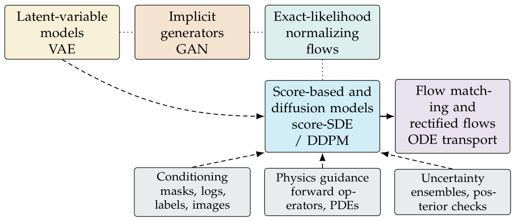
Figure 2.
Timeline anchors for generative modeling in geophysics. The milestones emphasize methodological adoption, benchmark availability, and the recent turn toward physics-guided diffusion priors.
Figure 2.
Timeline anchors for generative modeling in geophysics. The milestones emphasize methodological adoption, benchmark availability, and the recent turn toward physics-guided diffusion priors.
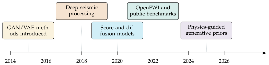

Table 1.
Application-method taxonomy used throughout this survey.
| Axis | Categories | Why it matters for geophysics |
| Generated object | Data, model, property, and hybrid spaces | A generated shot gather, velocity model, impedance volume, pore image, or latent posterior sample has different physical constraints and failure modes. |
| Model family | GAN, VAE, flow; denoising diffusion probabilistic model (DDPM); score stochastic differential equation (score-SDE); latent diffusion | The family determines likelihood access, sampling cost, mode coverage, uncertainty representation, and ease of physics coupling. |
| Conditioning interface | Unconditional prior, paired conditional mapping, classifier-free or metadata control, data-consistency guidance, posterior sampling | Conditioning determines whether the model is a simulator, a restoration tool, an inverse solver, or a prior embedded in a Bayesian workflow. |
| Physical coupling | Empirical data fit, operator-informed loss, differentiable solver loop, plug-and-play projection, rock-physics constraint | Geophysical credibility depends on consistency with acquisition geometry, wave physics, petrophysical relationships, and plausible geology. |
| Validation burden | Signal metrics, geological realism, downstream task performance, calibration, out-of-distribution testing, reproducibility | Visual or sample-level realism is insufficient; claims should survive physics checks, benchmark splits, uncertainty diagnostics, and open replication where possible. |
Table 2.
Cross-walk from the three application families to the taxonomy axes of Table 1. Entries name the dominant choices surveyed in each area and are tendencies rather than exclusive assignments; the physical-coupling and validation-burden axes of Table 1 are combined in the final column.
| Application family | Generated object | Dominant model family | Conditioning interface | Physical coupling and validation focus |
| Seismic processing | Data space: gathers, images, volumes | Score/DDPM and latent diffusion; GAN baselines | Acquisition masks and data-consistency guidance | Acquisition operators; spectra, coherence, residual leakage, and migration sensitivity |
| Inversion, VMB, and UQ | Model and property space: velocity, impedance | Diffusion priors and score-based posterior samplers; flow or ensemble baselines | Forward-model and likelihood gradients; geological or well priors | Wave-equation likelihood; posterior calibration, data residuals, and well or horizon coverage |
| Subsurface generation | Property and image space: pores, facies, logs, plumes | GAN priors and diffusion or latent diffusion | Conditioning data and rock-physics transforms | Flow and transport simulation; mass balance and blind-well or time-lapse validation |
Table 3.
Method families and their role in a geophysical generative workflow.
| Family | Primary object | Geophysical use | Main limitation |
| VAE | Latent variable and decoder | Compact representation, fast scenario generation | Blurry or over-regularized samples when the latent bottleneck is too strong |
| GAN | Implicit generator | Sharp seismic or model realizations under adversarial constraints | Mode coverage and uncertainty calibration are weak without extra checks |
| Normalizing flow | Invertible map and exact likelihood | Density estimation, posterior transforms, likelihood-aware priors | Invertibility and Jacobian constraints can restrict architecture choices |
| Score/DDPM | Denoiser or score over a noise schedule | Denoising, interpolation, reconstruction, posterior sampling | Many sampling steps and guidance-dependent calibration |
| Latent/conditional diffusion | Denoising in latent space with task conditioning | 3-D seismic restoration, inversion priors, multimodal constraints | Autoencoder and guidance errors can be hidden inside good-looking samples |
| Flow matching | Continuous velocity field between distributions | Fast transport paths and physics-constrained homotopies | Geophysical evidence is still sparse |
Table 4.
Seismic-processing use cases for generative or closely related deep restoration methods. The maturity column reflects evidence found for this section, not a final field-deployment recommendation.
Table 4.
Seismic-processing use cases for generative or closely related deep restoration methods. The maturity column reflects evidence found for this section, not a final field-deployment recommendation.
| Task | Representative sources | Maturity | Main survey caution |
| Denoising | Score/diffusion denoising and joint restoration [43,44,45] | Active diffusion literature | Generalization depends on noise class, acquisition domain, and blind field validation. |
| Interpolation and reconstruction | DDIM interpolation and constrained 3-D diffusion [31,44,51] | Active diffusion literature | Missing traces must be constrained by acquisition masks and coherence, not invented freely. |
| Super-resolution | Deep SR-denoising, CycleGAN enhancement, and SeisResoDiff [60,61,62] | Active but high-risk | Added bandwidth needs well, wavelet, phase, and amplitude checks. |
| Deblending | CNN deblending baseline [64] | Emerging for generative diffusion | Diffusion deblending remains an evidence gap in the surveyed literature. |
| Ground-roll attenuation | GAN/deep-learning ground-roll attenuation [72,73] | Established deep baselines, limited diffusion evidence | Must measure signal leakage and shallow amplitude distortion. |
| Data augmentation | Conditional GAN augmentation [74] | Useful support task | Synthetic examples must not contaminate real-only evaluation. |
Table 5.
Roles of diffusion and related generative models in seismic inversion and uncertainty quantification (UQ).
Table 5.
Roles of diffusion and related generative models in seismic inversion and uncertainty quantification (UQ).
| Role | Representative use | Main limitation for geophysical UQ |
| Direct velocity builder | Amortized map from gathers to velocity models; useful warm starts and fast ensembles [18,92]. | Calibration depends on training distribution, acquisition geometry, and field-data shift. |
| Learned FWI regularizer | Diffusion prior constrains acoustic or elastic FWI iterates [96,97]. | Produces plausible models, but not necessarily samples from a documented posterior. |
| Conditional prior | Geological, stratigraphic, or well information conditions the velocity prior [98]. | Can overstate certainty if sparse wells or interpreted horizons are treated as error-free. |
| Posterior sampler | Score or diffusion updates alternate with data-consistency gradients [12,39,105]. | Requires careful accounting of likelihood scale, modeling error, and the number of wave-equation solves. |
Table 6.
Subsurface-generation application clusters. Maturity labels indicate evidence volume and validation depth, not deployment readiness.
Table 6.
Subsurface-generation application clusters. Maturity labels indicate evidence volume and validation depth, not deployment readiness.
| Cluster | Representative sources | Maturity | Main validation requirement |
| Digital rock and pore-scale images | GAN reconstruction and stochastic limestone synthesis [113,114]; diffusion and latent diffusion pore images [115,116] | Active, moving from GANs to diffusion | Connectivity, morphology, and flow simulation must agree with real rock, not only image statistics. |
| Reservoir facies priors | Spatial GAN inversion and 3-D facies generation [14,117] | Established GAN evidence; limited diffusion evidence | Samples must honor conditioning data and preserve geological diversity outside the training image family. |
| Well logs and borehole images | Sequence GAN well-log generation and imputation [118]; conditional DDPM missing-log imputation [119]; image-log to core-image GAN translation [120] | Emerging, fast-moving | Blind-well tests, depth alignment, cross-log physics, and downstream petrophysical decisions are required. |
| CO2 and 4-D monitoring | 4-D seismic monitoring context [121]; plume GANs and diffusion forecasting [122,124,125]; Sleipner cWGAN reconstruction [123] | Active but not mature | Forecasts must satisfy pressure, mass-balance, seismic consistency, and blind time-step validation. |
Table 7.
Representative datasets and their benchmark roles.
| Resource | Typical use | Strength | Main reproducibility risk |
| OpenFWI and OpenFWI 2.0 | supervised FWI, elastic FWI, inverse-model pretraining | multiple synthetic families with explicit train/validation scale and published baseline metrics | overfitting to generator families; reporting aggregate scores without cross-family or out-of-distribution tests |
| Marmousi | velocity-model-building stress test and qualitative FWI comparison | canonical complex synthetic model with sharp lateral heterogeneity | reused crops, resamplings, and acquisition choices are often incomparable unless geometry and preprocessing are reported |
| SEG/EAGE-style salt examples | salt-boundary imaging, migration, interpolation, and inversion challenge problems | strong structural contrast and multipathing expose cycle skipping and spurious salt flanks | papers may cite the model name while using nonidentical smoothed, cropped, or simulated variants |
| F3 Netherlands offshore survey | real 3-D seismic interpretation, seismic-to-attribute or seismic-to-log experiments | public field data with seismic volumes, wells, horizons, impedance, and derived products | spatial leakage from adjacent inlines/crosslines, horizon leakage, and pretrained attribute leakage if products are mixed with raw seismic |
Table 8.
Metric classes that should be reported together rather than as a single scalar leaderboard.
Table 8.
Metric classes that should be reported together rather than as a single scalar leaderboard.
| Metric class | Examples | Interpretation caveat |
| Pointwise reconstruction | MAE, RMSE, relative , normalized data misfit | comparable for deterministic labels, but can penalize valid multimodal posterior samples |
| Structural similarity | SSIM, edge or horizon continuity scores | captures local structure better than MSE, but is still image-space and not geophysical validation |
| Distributional realism | embedding distance such as Fréchet Inception Distance (FID), spectrum and amplitude-distribution matching, facies or attribute histograms | depends strongly on the embedding; generic vision embeddings may be misaligned with seismic textures |
| Physics consistency | wave-equation residual, forward-modeled data misfit, amplitude-versus-offset (AVO)/angle consistency, well-tie error | requires the exact forward operator and preprocessing; otherwise it is not reproducible |
| Uncertainty quality | coverage of credible intervals, calibration curves, posterior sample diversity under fixed data | diversity alone is not uncertainty; samples must remain data-consistent |
| Operational utility | interpreter agreement, fault/horizon pick error, downstream inversion or monitoring improvement | should be evaluated on held-out surveys or blocked field regions when possible |
Table 9.
Baseline families needed before strong comparative claims are well-supported.
| Claim area | Baseline family | Risk if absent |
| Seismic denoising | Classical filters, supervised CNN or U-Net denoisers, GAN or self-supervised denoisers where relevant | Diffusion may be credited for ordinary gains caused by preprocessing or supervised capacity. |
| Interpolation and reconstruction | Prediction-error filters, low-rank or sparse methods, supervised deep reconstruction, GAN baselines, acquisition-mask ablations | Random masks can hide failure on coherent gaps, faults, or survey-scale missing swaths. |
| Resolution enhancement | Deconvolution, bandwidth extension, wavelet-aware methods, supervised super-resolution, well-tie and phase checks | Added high-frequency texture may be an artifact rather than recoverable signal. |
| FWI and inversion | Multiscale FWI, TV or Tikhonov regularization, learned amortized inverse maps, normalizing-flow or ensemble UQ baselines | Good image metrics can coexist with poor data fit or uncalibrated samples. |
| Digital rock and porous media | Process-based simulators, GAN/VAE/flow generators, pore-network or transport-property validation | Realistic pores are not enough if permeability, connectivity, or multiphase behavior drifts. |
| Well logs and monitoring | Geostatistical simulation, sequence models, Kalman or ensemble filters, physics or reservoir-simulation baselines | Samples can leak well identity, smooth anomalies, or overstate time-lapse detectability. |
Disclaimer/Publisher’s Note: The statements, opinions and data contained in all publications are solely those of the individual author(s) and contributor(s) and not of MDPI and/or the editor(s). MDPI and/or the editor(s) disclaim responsibility for any injury to people or property resulting from any ideas, methods, instructions or products referred to in the content. |
© 2026 by the authors. Licensee MDPI, Basel, Switzerland. This article is an open access article distributed under the terms and conditions of the Creative Commons Attribution (CC BY) license (http://creativecommons.org/licenses/by/4.0/).
Copyright: This open access article is published under a Creative Commons CC BY 4.0 license, which permit the free download, distribution, and reuse, provided that the author and preprint are cited in any reuse.


