
Submitted:
24 June 2026
Posted:
25 June 2026
You are already at the latest version
Abstract
The Susceptible-Infected-Recovered (SIR) model is a crucial framework for researching the dy-namics of infectious diseases within humans. Here, we provide an overview of both analytical and numerical methodologies for solving the SIR model. This model contains a set of ordinary differential equations that govern the dynamics of infectious disease which represent the rates of change for susceptible, infected, and recovered humans across time. In order to comprehend the transmission and management of infectious diseases, analytical and numerical solutions are complimentary. Analytical solutions provide theoretical predictions and insight into the model's underlying dynamics, while numerical solutions give the simulation and investigation of the model's behavior under many situations. We can understand the dynamics of infectious diseases and public health initiatives to lessen their effects by integrating these methods. To demonstrate their accuracy in forecasting the spread under varied conditions, this study offers trustworthy so-lutions to the differential equations regulating dengue transmission.
Keywords:
dengue disease
; SIR model
; exact solutions
; Euler method
; RK4 method
1. Introduction
Infectious diseases have been accounted for to be the most common cause for a high rate of mortality during recent years. By the end of the twentieth century, considerable advances had been made in the understanding and treatment of diseases, particularly owing to vaccines, antibiotics and improvements in living standards. These interventions were regarded as essential for the control of the transmission of infectious agents. Nevertheless, the eradication of such diseases has remained a daunting challenge [1]. In developed countries, the battle with infectious diseases was overlooked in favor of cancer and other degenerative diseases. Therefore, by the onset of the new century, countries in the third world still suffered great losses because of infectious diseases. Malaria, yellow fever, even AIDS and Ebola, have been, if not eradicated, then clearly active elements in the canvas of world history [1,2].
Despite the remarkable progress in medical science, these diseases inflict unbearable sufferings, high mortality. These problem are disproportionate, as a critical prerequisite for global efforts. Perpetual endeavors to address such public health issues is cooperation because it’s the issue for the entire globe. Southeast Asia registers dengue fever as the second most prevalent viral pandemic and it’s gaining momentum in other tropical nations.
Dengue illness, caused by Aedes genus mosquitos, can present in two forms: Dengue Fever (DF) regarded as the classical dengue and Dengue Hemorrhagic Fever (DHF) which can lead to the serious and life threatening Dengue Shock Syndrome (DSS). Dengue disease is very complicated due to its four different serotypes to include: DEN1, DEN2, DEN3 and DEN4. Upon infection by one serotype, one acquires homologous immunity to that specific serotype hence remains susceptible to any infection by the other serotypes. This type of protection loses its value after a period of approximately 12 weeks which then allows the individual to be infected by the rest of the serotypes. This phenomenon, referred to as heterologous immunity, significantly increases the risk of suffering from Dengue Hemorrhagic Fever (DHF). The wide spread of Dengue fever along with its complex immunological interactions poses a great threat to population health in the tropical regions. In order to limit and decrease the risk of ever contracting Dengue fever, an appropriate framework which incorporates mosquito control strategies, vaccine development and health promotion should be employed. Battling this ever looming threat to human health on a global scale is the need to untangle the complex relationship existing between the virus and the human immune system [3].
Dengue fever, this disease also known as ‘Break bone fever’, is caused by dengue viruses with sudden onset fever and severe headaches where the bone behind an 82% of people suffering from it feels as if breaking. Classic dengue fever goes hand in hand as the most common strain, anywhere from infections this disease consists to respiratory [4]. A patient suffering on average between two weeks may display such symptoms. In regions with high population density, the augmented form slipping under the radar could be due to DOMID (dengue receptors). The most lethal MPO biotropic form DHF is accompanied by such symptoms as abrupt fever coupled with persistent nausea, vomiting, and sleepiness due to low blood pressure, often caused by dehydration. Medically, these symptoms may lead a situation within days which could potentially kill a patient.
Preventing Dengue or secondary infectious diseases is crucial because these are the possible causes of conditions which progress to such DHF [5]. There have been much efforts put in regard to survey dengue fever via controls. Hit and run strategies involving insecticides have time and time again invariably returned a failure. And the progression endemic of dam really so limitization was worsened by ecological degradation due to rapid urbanization and unsanitary conditions like many other infectious diseases. There are no such measures using mosquitoes as ‘control’ that will work unattended to.
Strategies like improved sanitation, urban development, health education and building hospital capacity avoid the transmission and impact of this ailment. The only way it seems that the devastating burden of dengue fever can be mitigated is by the combination of multiple approaches. As opposed to malaria, which is encountered in rural areas and is transmitted using organisms (mosquitoes), dengue fever is contracted due to the contact between susceptible individuals and mosquitoes of the Aedes genus that can cause one of the four serotypes of dengue virus. In particular, it is known that the Aedes aegypti and the Aedes albopictus are the two most active species in the transmission of Dengue fever. Since Aedes aegypti is small led, it prefers urban centers where crowding is a norm, and the species’ bites occur mainly during daylight hours. Meanwhile, the Aedes albopictus prefers more of rural habitation.
Dengue fever has a number of threats associated with it. To begin with, its frequent connection with the global travel makes it easy for this disease to gain spread and further aggravate its consequences due to having multiple serotypes. This burden can be illustrated through absenteeism and reduced productivity and cost of seeking medical care and treatment. In addition, it is possible for residents to progress from dengue fever to more severe forms including dengue shock syndrome and dengue hemorrhagic fever [4].
Making great financial investments do not only concern these diseases as they are a curse against human life. Such extreme manifestations of the disease’s evolution can bring disaster and unnecessary health impairment impact. However, dengue fever has been shown to require a complete program that encompasses vaccine drives, mosquito control, and other measures to improve the health system and educate people about public health. By doing so, the impact of the disease will be reduced which in turn minimizes the economic and social burden that accompanies dengue fever [6].
In this article we simulate the transmission dynamics of dengue virus numerically using the SIR model. Such numerical results could capture the interactions that command a relationship between the susceptible, infectious, and recovered, using Euler’s method [7], Runge-Kutta methods [7,8]. More importantly, employing numerical methodologies could allow us to explain dengue epidemics in a more realistic manner by integrate regional heterogeneity, demographic parameters, and vector dynamics [4].
At the same time, the SIR model’s analytical solutions have also demonstrated the basic dynamics of the transmission of dengue. To highlight the factors behind the outbreak of endemic sites, epidemic threshold values and their control mechanisms, fitness determination has been attempted in equilibrium points [9], stability analysis [9]. Furthermore, analytical solutions help to enhance our understanding of the dengue transmission dynamics by making the analysis more rigorous and straightforward. In recent years, the importance of integrating two philosophies in dengue studies is increasing: analytical and numerical approaches.
Varying transmission dynamics of Dengue may be addressed more effectively by analytical methods combined with numerical data. Also, some emerging trends in computational techniques, high performance computer and machine learning algorithms may as well enhance the accuracy of forecasting Dengue disease and the predictive value of mathematical models. In this manuscript we will present dengue illness focusing on most recent advances in the numerical and analytical approaches to solving the SIR model.
We expect our study to help identify new tendencies, resolve current issues, and recommend ways for further research on the basis of the integration of results from a variety of studies. In conclusion, the objective of this review is to find a way how the fight against dengue hemorrhagic fever could be strengthened and the world health problem minimized. The model emphasizes important features like infection rates, recovery rates and vector mortality and demonstrates how these determine and change the basic reproduction number and disease dynamics.
2. Materials and Methods
The mathematical model is applied for the description of the transmission patterns of serotype 1 of dengue virus in both the human and the mosquito [10,11]. This model is based on the concepts of infectious disease epidemiology, in particular the Susceptible, Infected, and Recovered (SIR) model. In this configuration, the SIR model recognizes the following strata: the human population ( ) and the vector population ( ). Humans are classified as virus holders into three divisions. – the susceptibility to dengue infection, – the infection stage and – the dengue recovered stage. The same pattern exists with regards to the vector which consists of mosquitoes, them being also divided into two groups, susceptibility stage in mosquito, infective stage in mosquito. The division essentially allows the human and mosquito together into the disease dynamics.
This particular model works on the basis that some people in the human target group have already been infected and some have never had the virus before. It also assumes that the propagation of the virus infection goes higher in the human body while at the same time the animal vector does not change. The treatment was the same for both humans and mosquitoes as homogenous units.
We propose a mathematical model that can predict the dynamics of transmission of three compartments in the human(host) and dynamics of transmission of two compartments in the mosquito in order to comprehend the transmission and outbreak of dengue diseases. For this reason, we consider
: Number of human size, : Number of susceptible in human size, : Number of infective in human size, : Number of recovered in human size, : Number of mosquito size, : Number of susceptible in mosquito size, : Number of infective in mosquito size
The comprehensive dynamics of both human and mosquito groups can be encapsulated within a mathematical model of host-vector interaction, formulated through nonlinear differential equations [11,12]. These equations describe the interplay between the various human groups and their interactions over time.
For human,
For mosquito
With conditions and
Where, birth/death ratio in the human of the host,
mortality rate in the human of vectors,
Transmission probability from vector to host
Transmission probability from vector to host
Recovery rate in the host human
biting rate of vector
A=Recruitment rate
Non dimensionalization form:
To non-dimentionalize the mathematical model we assume the following transformation
and
Using theses transformations, the system of the above equations (2.1) as follows
For human,
Similarly, we get
For mosquito, from (2.2) we get
With conditions,
and
The above system of differential equations for human and mosquito can be written as
For the simplification of the above model let us consider ; ; then the above equation (2.3) becomes,
3. Mathematical Analysis of the Model
To understand the local dynamics of the system of differential equations [2,13], we find the equilibrium points by solving the following system of differential equations
By solving the above system of equation (3.1) We identify the system's disease(infection)-free equilibrium point (DFE), when illness compartments are treated as zero. In the model (2.4), there are others compartments, of which there are two infected compartments, i.e., and , and two uninfected compartment, i.e. , and one recovered compartment i.e. . At the steady state without infection = =0. So, the disease(infection)-free equilibrium point (DFE) is ( , )=(1,0,0,1,0,) which is denoted by . we also identify the system's disease endemic equilibrium(DEE) point, when the disease spreads among the human. It is denoted by , , ). If we summarize the equilibrium points it can be written in the following form,
1. Stability analysis of the model at equilibrium points
In this section, we use the linearization method to understand the stability of (3.4) at respective equilibrium points [14,15]. The Jacobian matrix for the above model is,
2.1. Stability Analysis at Disease Free Equilibrium Points
The Jacobian matrix at disease free equilibrium points denoted by , the Jacobian at the first equilibrium point is as follows [16]:
At the equilibrium point the eigen values are given below:
Using parameter values are given in Table 1. The eigen values for eq. (3.1) are as follows,
Since one of the Eigen values is positive, the equilibrium point is a saddle point. Therefore, there is no infected human with dengue. There are no diseased people in the population, and people are generally healthy.
2.2. Stability Analysis at Endemic Equilibrium Points
The Jacobian matrix at endemic equilibrium points denoted by , the Jacobian at the first equilibrium point is as follows:
Using parameter values are given in Table 1. The Eigen values for eq. (4.1) are as follows
; as the eigenvalues are complex and negative, the equilibrium point is asymptotically stable. The equilibrium point will be steady, and there will be some cases of dengue fever.
2. Reproduction Number
In the context of epidemic disease models, the basic reproduction number ( plays a crucial role in predicting the potential for disease transmission within a population. Denoted as , it is defined as the average number of secondary infections produced by a single infected individual in a fully susceptible population. More formally, is the ratio of newly infected individuals to the total number of infected individuals, reflecting the rate at which the disease spreads [17].
The basic reproduction number is a critical concept in epidemiology, as it helps determine whether a disease will persist or eventually die out. If >1 ,each infected individual is, on average, responsible for more than one new infection, leading to a sustained outbreak or epidemic. On the other hand, if <1, the disease is unlikely to persist and will eventually die out [18].
In the specific disease model under consideration (model 2.4), the spread of the infection is driven primarily by interactions between the susceptible population and the infected individuals. These two groups—susceptible individuals and infected individuals—play an essential role in the transmission process. Notably, the model assumes that recovered individuals do not contribute to further transmission of the disease. This assumption implies that once individuals recover, they no longer participate in the infection dynamics, and therefore, there is no "recovery to susceptible" pathway in the model.
Thus, the basic reproduction number provides a threshold that helps assess the future trajectory of the disease within the population, and its value is influenced by the dynamics between susceptible and infected individuals, but not by recovered individuals.
Therefore, to find out the basic reproduction number of the model, we consider the equations of system (2.4) as follows
From (5.1), we can form the following matrices F and V for gain and loss terms [19] respectively
At the disease free equilibrium point, , we find
Eigen values of are
Therefore, the basic reproduction number,
3.1. Boundedness and Non-Negativity of Solutions
Theorem 6.1 : The feasible region is positively invariant for the model (2.4) with the initial condition defined by Proof: For human,
Let, the size of the entire human beings is where . Then the increase rate of entire human is . From the system (2.4), we find
For large time , the affected human passes away. So, we get
Therefore, we write which indicates that ,i.e., 1 is the supremum of .
For mosquito,
Let, the size of the entire mosquito is where . Then the increase rate of entire human is . From the system(A), we find
For large time , the affected human passes away.
From the above equation, we get,
Therefore, we write which indicates that ,i.e., 1 is the supremum of .
Theorem 3.2 : The solution of the system (2.4) is positive and bounded for all . for all Proof. To demonstrate the solution's positivity, we need to show that on any hyperplane enclosing the positive vector space from the system (2.4),
So, the system (2.4) solution is positive.
4. Numerical Solution of SIR Model
The exact solution of SIR model is not always possible; therefore, we solve the model by using different numerical approach. In this article we use Euler method and RK4 method as a numerical technique to solve the dengue dynamics.
7.1. Algorithm of RK4 Method
Suppose , we have m differential equations:
With initial conditions
There is no derivative on the right hand side and all of these m equations are of order one.RK4 formula is as follows:
Where,
Where, is the RK4 approximation of and h is step size.
5. Algorithm of Eulers Method
The Euler method is used to solve a system of nonlinear equations
… …. ….
With initial conditions and choose a fixed h value that is h=
…….
7. Numerical Simulation
This simulation uses the debris of dengue data from January 2024 to March 2025 in Dhaka city [20]. As the city is most populated, Bangladesh is concerned about the dengue outbreak. One such estimate puts the figure to around 23.9 million residents in Dhaka in the first month of 2024 [21]. Dhaka's heavy summer monsoon rains provide the ideal conditions for the breeding of dengue since the vector population multiplies rapidly in stagnant waters. For most of the regions of the country, the mean temperature for the year of 2024 was above the average thus enabling development of the dengue. The dengue disease data including four years of Aedes infection statistics came from the Health Emergency Operation Center and Control Room in Dhaka. The average parameter values of the mosquito population are assumed to be a certain constant value to approximate the values. This SIR model population simulation of the disease goes by the following parameters:
7.1. Simulation of Dengue Dynamics for Different Transmission Rate (
In this section, we observe the effects of different parameters which are used in our model. In the numerical experiments, a single parameter is altered while keeping all other parameters constant to observe its influence. For variations of transmission rate , we simulate the dengue dynamics for susceptible, infected, recovered human.
In Figure 1 , the parameter (the human-to-vector contact rate) is varied, with all other parameters held fixed. The analysis is performed for three different values of . The impact on the populations of susceptible humans, infected humans, and infected vectors is presented in the figure.
Key findings include the following:
- As the value of increases, the number of infected humans rises, accompanied by an increase in the population of infected vectors.
- The susceptible human population declines more rapidly and approaches nearly zero for higher values of
- Conversely, a decrease in the
value results in fewer infected humans, which can be attributed to a reduced population of infected vectors. This leads to a slower transition from susceptible to infected humans.
These results highlight the critical role of the human-to-vector contact rate in shaping the dynamics of dengue transmission.
6.2. Simulation of Dengue Dynamics for Reproduction Number
The Reproduction number is used to measure the possible communication of a disease. The shows the number of infection among the humans as result of infected mosquitos. The formula of reproduction number as discussed in section (Reproduction number) is,
Using the parameters in Table 1 for Dhaka city the reproduction number can be calculated as,
The above figure illustrates how the reproduction number affects the dynamics of dengue transmission. In Figure 2, For ≤1, the infected population declines, and the disease dies out. In Figure 2, For >1, the disease spreads, with higher values leading to a larger and earlier peak in the infected population. This highlights the importance of maintaining ≤1 through interventions such as mosquito control and vaccination to prevent outbreaks.
6.3. Simulation of Dengue Dynamics Using Different Numerical Method
In order to investigate the dynamics of the model, we perform numerical simulations of the model as a standard Initial Value problem (IVP) (4.1) incorporating a relevant initial condition.
For numerical solution of the IVP (4.1), we use Runge-Kutta fourth order(RK4) and Eulers method. The initial conditions are chosen from the dataset as we also take the parameter values from table and the reproduction number, =0.08(<1).
Numerical simulations employing Exact methods, Euler's method, and the Runge-Kutta fourth order (RK4) method offer diverse insights into modeling various human dynamics [22]:
The Exact solution of the SIR model shown in Eq. (4.1) is then compared to the results obtained from the Euler and RK4 methods. The initial conditions are and the parameters values from the Table 1 . The Figure 3 shown above, says that the two solutions to the SIR model disclosed by Euler and RK4 methods agree well with the exact solution for a step size of Therefore, it can be concluded that both methods were found to yield trustworthy results in solving simplified nonlinear dynamical models.
Figure 3.
Comparison of exact solution with RK4 and Euler Method (Left: susceptible and Right: Infected).
Figure 3.
Comparison of exact solution with RK4 and Euler Method (Left: susceptible and Right: Infected).
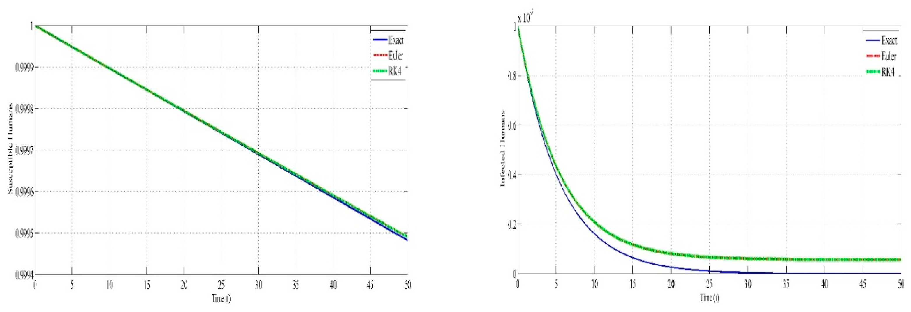
Figure 4.
Comparison of dengue dynamics with Exact and Euler Method.
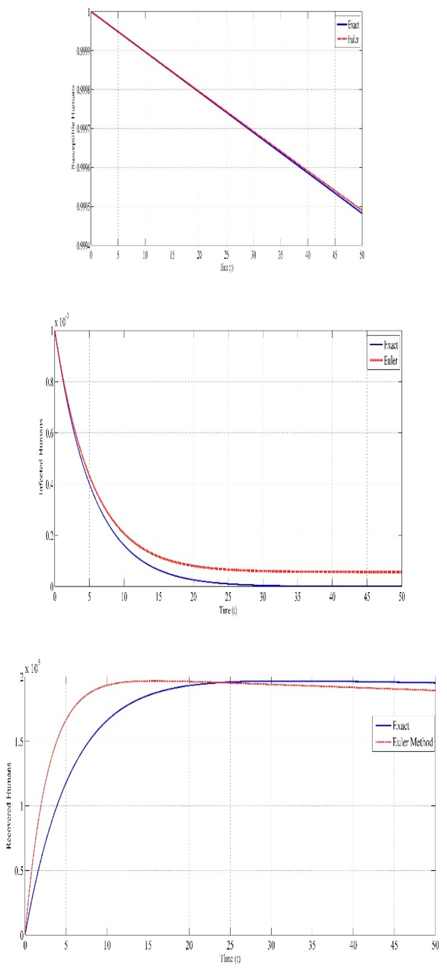
The blue line (Exact method) and red dashed line (Euler method) are nearly identical, indicating close agreement between the methods. This suggests that the Euler method provides a good approximation of the exact solution for the dynamics of susceptible humans. In this case for infected human, the two methods show some visible differences, particularly at the initial stage of the outbreak. The Euler method (red dashed line) slightly overestimates the number of infected humans compared to the Exact method (blue line). However, the divergence diminishes over time as the infection stabilizes. The curve for recovered humans shows a smooth and steady increase over time. The recovery rate increases consistently as the infection decreases and fewer people remain infected. Over time, the Euler method's curve for recovered may either slightly overestimate or underestimate the recovered population compared to the Exact solution.
The first panel of Figure 5 portrays the dynamics of the susceptible human population. Both methods track each other closely during the observation period, wherein the susceptible population decreases progressively as people become infected. RK4 provides a good approximation to the Exact solution, showing minimal deviation. The very few discrepancies that may present express the error incurred with the numerical approximation of the RK4 method, though always remaining small. The second panel of figure 5 shows the infected human population reacting very sharply at first, reaching a peak, and declining with time as the infected recover or die. Once again, both methods follow similar trajectories, except that the RK4 method might show small deviations from the Exact solution, especially near the peak of the infected curve. These deviations may be more pronounced for more complicated or sensitive models; however, generally speaking, the RK4 method produces a reasonable approximation. From time to time, there is actually a tip of the balance in favor of one method or another, hence small variations intervened. The third panel of figure 5 illustrates recoveries: the recovered human over time growing by new recoveries. Both methods have an increasing number of recoveries. And once again, this curve closely fits the RK4 solution, which indicates that the RK4 method does, indeed, give a valid approximation for the dynamics of recovery. Differences, which were slight, appeared if at all in early times when the number of recoveries was still small.
The Figure 6 illustrates the solutions of the dengue dynamics for Susceptible (S), Infected (I), and Recovered (R) human in the SIR model, using three methods: Exact, Euler, and RK4 (Runge-Kutta 4th Order). These methods provide a benchmark solution for the spread of dengue within a population. The blue line which represent susceptible human shows a steady decline, reflecting the diminishing number of people who are vulnerable to infection. The red line which represent infected population follows the typical epidemic curve, rising sharply to a peak as the disease spreads and then declining as individuals recover or are removed from the infected category. The curve illustrates the outbreak's progression by showing the epidemic's peak and subsequent decline. As the virus diminishes the green line, which represents recovered humans, rises gradually and becomes closer to an asymptote, signifying the outbreak's end and the population's eventual stabilization.
7. Conclusion
As it aids in the comprehension of transmission dynamics and the efficient execution of disease control, the control of dengue outbreaks through the application of SIR (Susceptible–Infected-Recovered) models is of great importance. Recent computational methods, including Exact, Euler and RK4 (Runge-Kutta 4th Order methods) have been utilized in the simulation of the dynamics of the susceptible-infected-recovered human populations, and the reproduction number (R₀). The control of the rate at which the population becomes sick - the βₕ, has also been varied and the effects on the epidemic dynamics documented. The Exact approach gives the most wide-ranging solution to the problem at hand by looking at the dynamics of the susceptible, infected and the recovered over time. Because of this simple reason alone, it becomes possible to measure the reproduction number (R₀) accurately, which is a critical parameter needed to estimate the potential extent of an eventual outbreak. It was shown that the Euler technique, a simpler numerical method, was able to successfully capture the dynamics of the epidemic with reasonable precision. The magnitude of variation caused by the Euler technique were not particularly significant but rather small – more so in the later stages of the epidemic or during periods of rapid transition such as the peak of the infection. However, even with its computational efficiency, these variances underscore the weaknesses of the Euler modeling technique in simulating epidemics with complicated patterns over long timelines. By virtue of its high precision, the results using RK4 approaches were almost equal to the Exact method, especially in predicting the transitions of the susceptible-infective-recovered population. The RK4 method compared to the Exact solution has quite small deviations and is comfortable because of the fourth order accuracy. Given the requirements for a more detailed representation of the dynamics of dengue, this method is better than the Euler technique as it optimally strikes the required level of detail along with efficiency. The reproduction number (R₀) is a significant telemetric that portrays the chances of transmitting infectious diseases. R₀ is highly sensitive to the parameter changes in transmission coefficient (βₕ). Values of R₀ are repetitively estimated using the Exact, Euler and RK4 methods with the Exact method being the most effective. Increasing the transmission coefficients βₕ raises the reproduction number and thus, an increase in the number of new cases observed following reproduction number increase leads to more rapid spread. Variations in R₀ are estimated by both the Euler and RK4 methods; however, results of the latter are more accurate owing to precision within the method. The study demonstrated that variations in the βₕ values of the transmission coefficient which refers to the rate of spreading of a particular pathogen amongst susceptible individuals influences the dynamics of outbreaks. The dynamics of infection in a population change as higher values of βₕ are associated with quicker transmission which causes a higher overall proportion of infected people and earlier peak in infections. Such has been the trend as the βₕ value changed during the course of the epidemics being analyzed by Exact, Euler and RK4 techniques which appeared in that order but once more, RK4 presented the most precise representation of these dynamics.
Finally, the advantages and weaknesses of the Euler, RK4 and Exact methods in terms of their applicability within the context of an SIR model-based simulation of dengue epidemics are shown. The industry relies heavily on the industry standard Exact approach for precision purposes while sacrificing some degree of precision for the more basic, quicker and more cost-effective method; the Euler methodology. With its high level of accuracy and dependability, there is no question that the RK4 method is the best suited for the dengue epidemic simulations requiring high detail. Likewise, highlighting the effectiveness of βₕ and R₀ in determining the characteristics of the epidemic, the research emphasizes the complexity of algorithms needed in order to implement disease control strategies effectively.
Funding
self-funding.
Acknowledgments
I would like to thank my supervisor Prof. Dr. Mohammad Osman Gani for supporting the entire work.
Conflicts of Interest
The authors declare no conflicts of interest regarding the publication of this paper.
References
- "Johansson MA, Powers AM, Pesik N, Cohen NJ, Staples JE. Nowcasting the spread of chikungunya virus in the Americas. PLoS One. 2014;9(8):e104915.". [CrossRef]
- " Side, S. and Noorani, M., A SIR model for spread of dengue fever disease (simulation for south sulawesi, indonesia and selangor, malaysia), World Journal of Modelling and Simulation, 9(2), 96–105, 2013.".
- "Lee L., Population of aedes aegypti dengue, Interview; 2009.".
- "Koizumi T, Yamaguchi K, Tonomura K. An epidemiological study of dengue fever, Taiwan J Med Assoc Formosa 1917," vol. 176:369–92.
- " WHO, Dengue and severe dengue, http://www.who.int/mediacentre/factsheets/ fs117/en/ January 2012.".
- "Codeço, C. T. (2001). "Endemic and Epidemic Dynamics of Dengue: Challenges for Vector Control." Annals of the New York Academy of Sciences, 954(1), 308-311.".
- " Yulius Keremata Lede ; Sudi Mungkasi .“Performance of the Runge-Kutta methods in solving a mathematical model for the spread of dengue fever disease”, International Conference on Science and Applied Science(ICASA)2019, AIP Conf. Proc. 2202, 020044 (2".
- " J.Y. Wijaya, T.H. Liong and K.R.R. Wardani, “Perbandingan penyelsaian persamaan diferensial biasamenggunkan metode back propagation, Euler, Heun, dan Runge-Kutta order 4.”,in Indonesian Language, Journal Telematika, 11,1-6(2016).".
- " Javeed S, Ahmed A, Khan MS, Javed MA. Stability analysis and solutions of dynamical models for dengue. Punjab Univ J Mathem 2018; 50(2):45–67.".
- " Lopez, L., CESMAG, I. U., Loaiza, A. and Tost, G., A mathematical model for transmission of dengue, Applied Mathematical Sciences, 10(7), 345–355, 2016.".
- "Esteva, L. and Vargas, C., Analysis of a dengue disease transmission model, Mathematical biosciences, 150(2), 131–151, 1998.". [CrossRef]
- " Esteva, L. and Vargas, C., Coexistence of different serotypes of dengue virus, Journal of mathematical biology, 46(1), 31–47, 2003.". [CrossRef]
- " Guo, S., Li, X. and Ghosh, M., Analysis of a dengue disease model with nonlinear incidence, Discrete Dynamics in Nature and Society, Hindawi, vol. 2013, 2013.". [CrossRef]
- " Alam M, Saha S, Nafiujjaman M. Stability and bifurcation analysis of a three-dimensional dengue epidemic model with saturated incidence rate. Chaos Solitons Fractals. 2019; 121:37-50.".
- "Javeed S, Ahmed A, Khan MS, Javed MA. Stability analysis and solutions of dynamical models for dengue. Punjab Univ J Mathem 2018; 50(2):45–67.".
- " Javeed S, Ahmed A, Khan MS, Javed MA. Stability analysis and solutions of dynamical models for dengue. Punjab Univ J Mathem 2018; 50(2):45–67.".
- "Puspita, J. W., Fakhruddin, M., Fahlena, H., Rohim, F. and Sutimin, S., On the reproduction ratio of dengue incidence in Semarang, Indonesia 2015-2018, Communication in Biomathematical Sciences, 2(2), 118–126, 2019.". [CrossRef]
- " Hethcote, H., The mathematics of infectious diseases, SIAM review, 42(4), 599–653 2000.".
- "https://mpra.ub.uni-muenchen.de/114390/1/MPRA_paper_114390.pdf".
- "https://dashboard.dghs.gov.bd/pages/heoc_dengue_v1.php".
- "Institute of Epidemiology Disease Control and Research (IEDCR), B.E newsletter on dengue, December 2024.".
- " Hu, Z., Ma, W. and Ruan, S., Analysis of SIR epidemic models with nonlinear incidence rate and treatment, Mathematical biosciences, 238(1), 12–20, 2012.". [CrossRef]
- "International Journal of Computer Applications 118(21):1-4".
- " Bamouh A, Zouagui Z, Rachik M. Analytical and numerical solutions of a model for dengue fever with vertical transmission. Heliyon. 2018;4(11):e00992.".
- "https://www.researchgate.net/publication/366453979_Stochastic_Bayesian_Runge-Kutta_Method_for_Dengue_Dynamic_Mapping".
- " Perkins TA, Siraj AS, Ruktanonchai CW, Kraemer MUG, Tatem AJ. Model-based projections of dengue fever in Bangladesh: a joint analysis with climate and non-climate risk factors. Environ Health Perspect. 2020;128(9):97002.".
- " Rodrigues FAS, da Silva MB, Gurgel FAS. Dynamics and control of dengue transmission with an imperfect vaccine. Appl Math Model. 2017;45:192-207.".
- "Sissoko FG, Eitrem R, Traore AK, Øyeflaten I. A deterministic SEIR model for dengue fever transmission dynamics in the West African region: a sensitivity analysis. J Trop Med. 2020;2020:1-14.".
- "Alam M, Saha S, Nafiujjaman M. Stability and bifurcation analysis of a three-dimensional dengue epidemic model with saturated incidence rate. Chaos Solitons Fractals. 2019;121:37-50".
- A model for chagas disease involving transmission by vectors and blood transfusion.
- Ozair, M., Lashari, A., Jung, I. and Okosun, K., Stability analysis and optimal control of a vector-borne disease with non linear incidence, Discrete Dynamics in Nature and Society, 2012.
- " Braselton, J. and Bakach, I., A survey of mathematical models of dengue fever, Journal of Computer Science Systems Biology, 8(5), 255, 2015.".
Figure 1.
Effect of transmission rate on dengue dynamics(susceptible, Infected, Recovered).
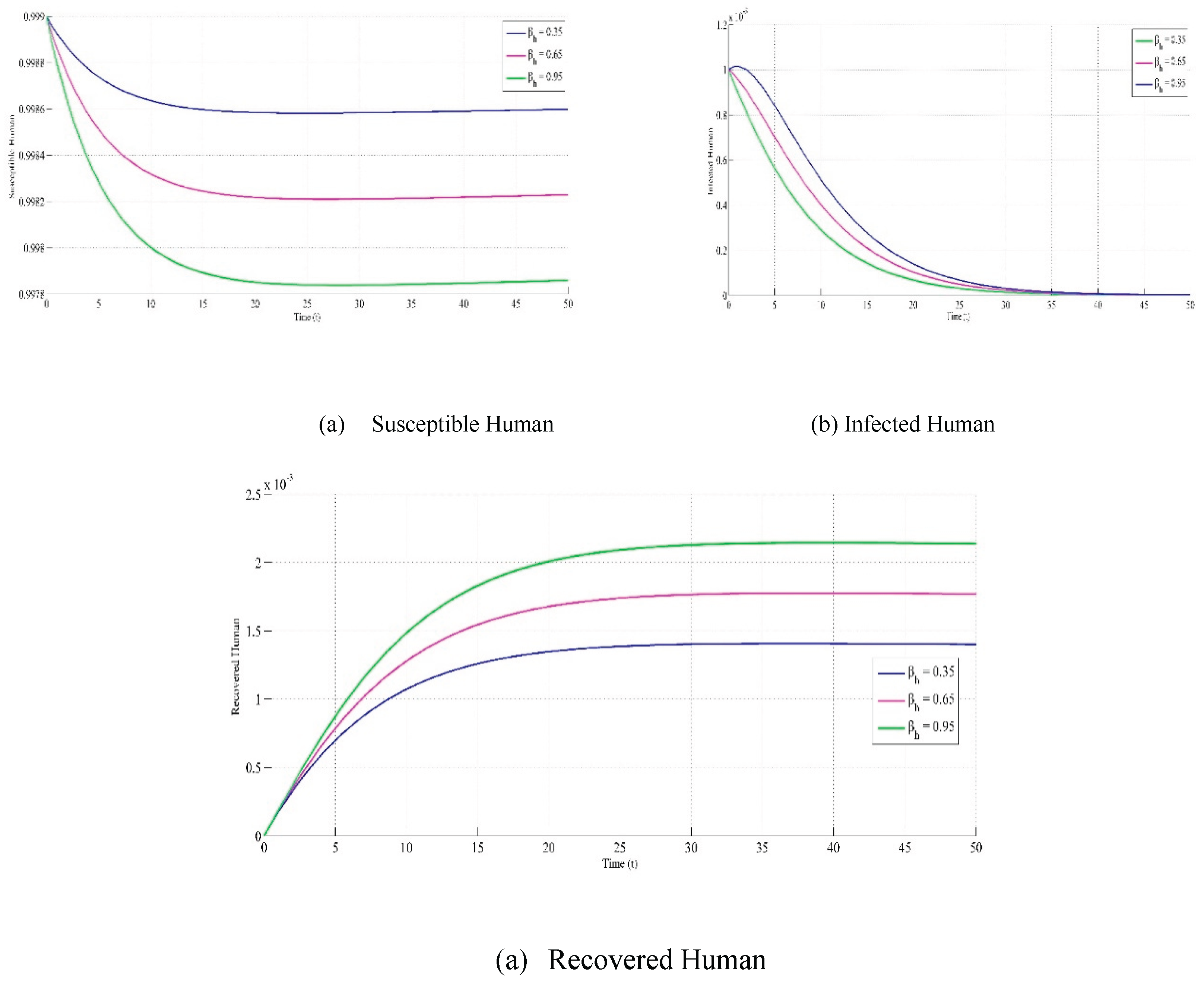
Figure 2.
Left: Dengue Transmisson Dynamics( >1) with . Right: Dengue Transmisson Dynamics( <1) with
Figure 2.
Left: Dengue Transmisson Dynamics( >1) with . Right: Dengue Transmisson Dynamics( <1) with
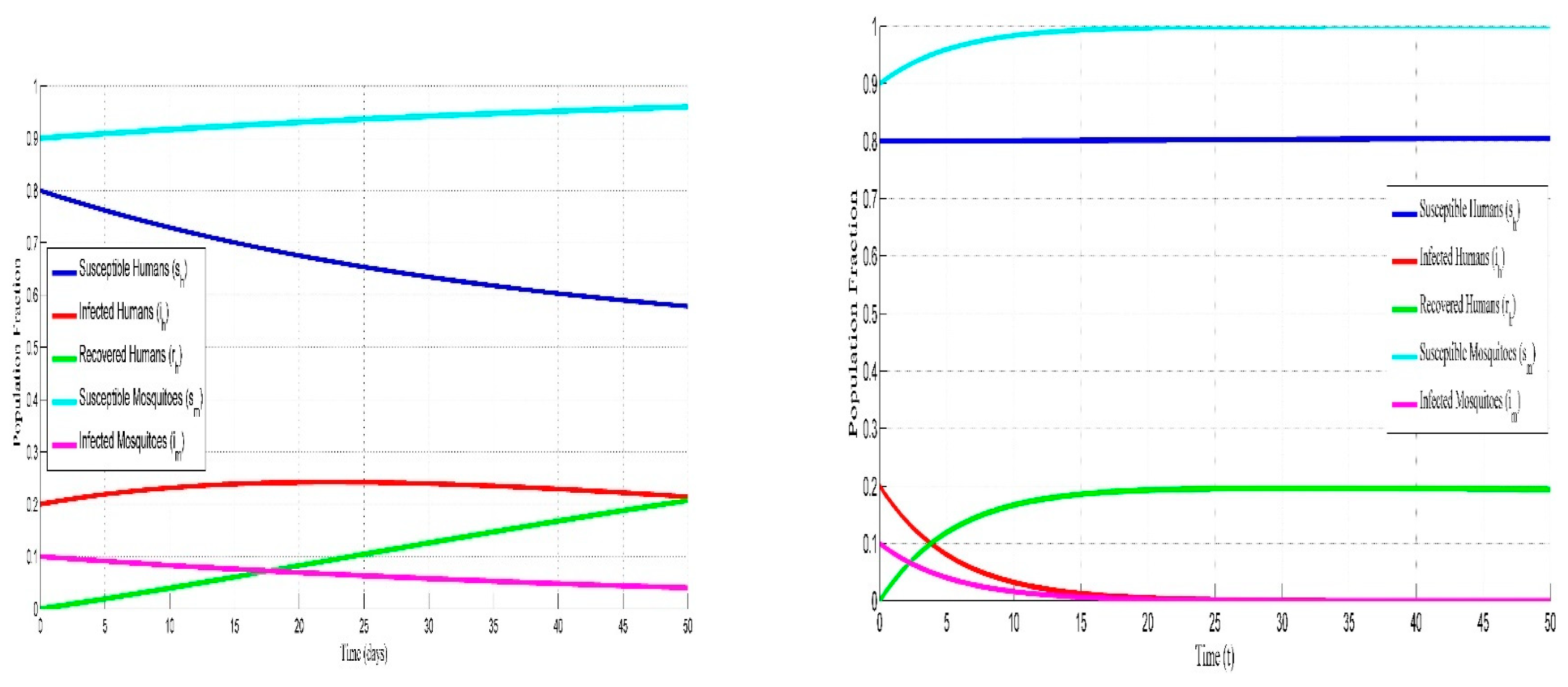
Figure 5.
Comparison of dengue dynamics with Exact and RK4 Method.
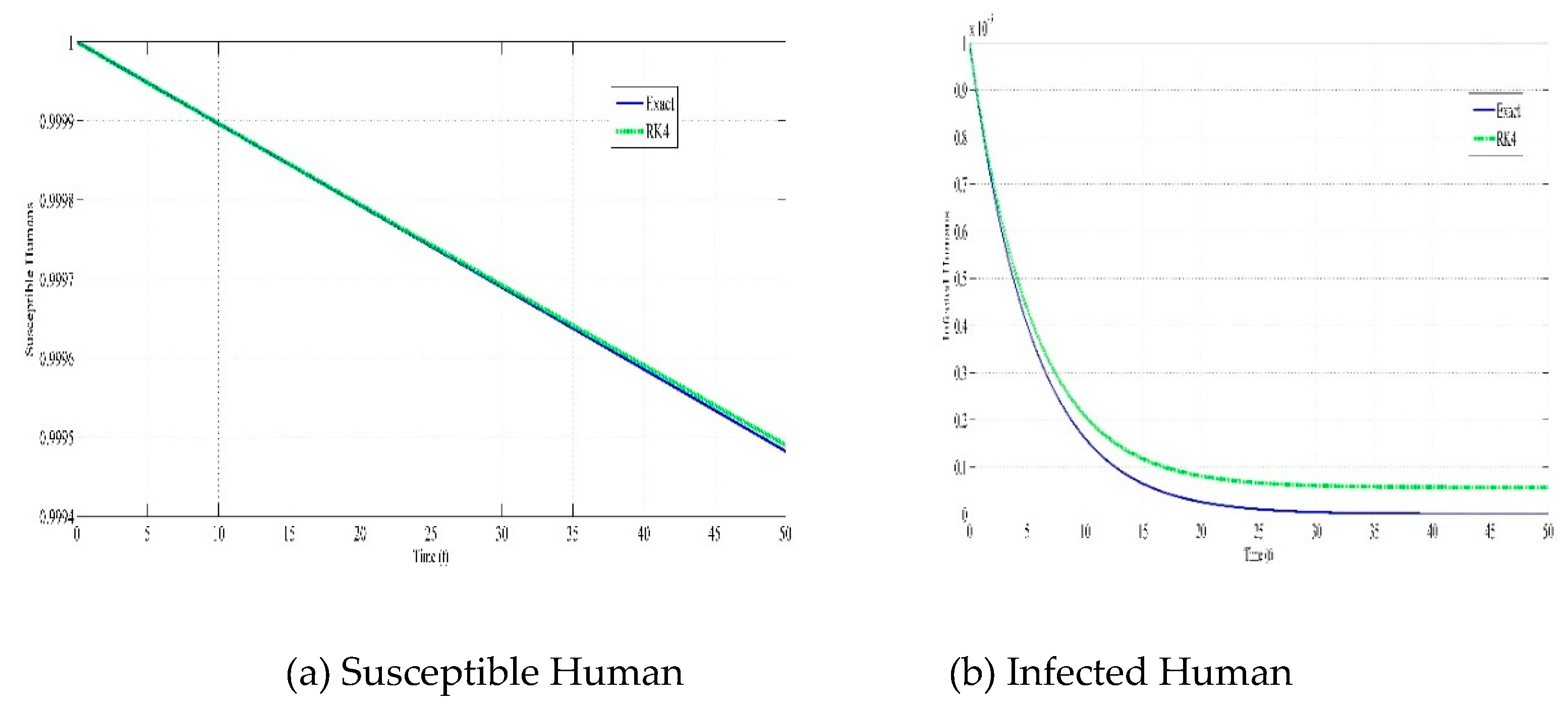
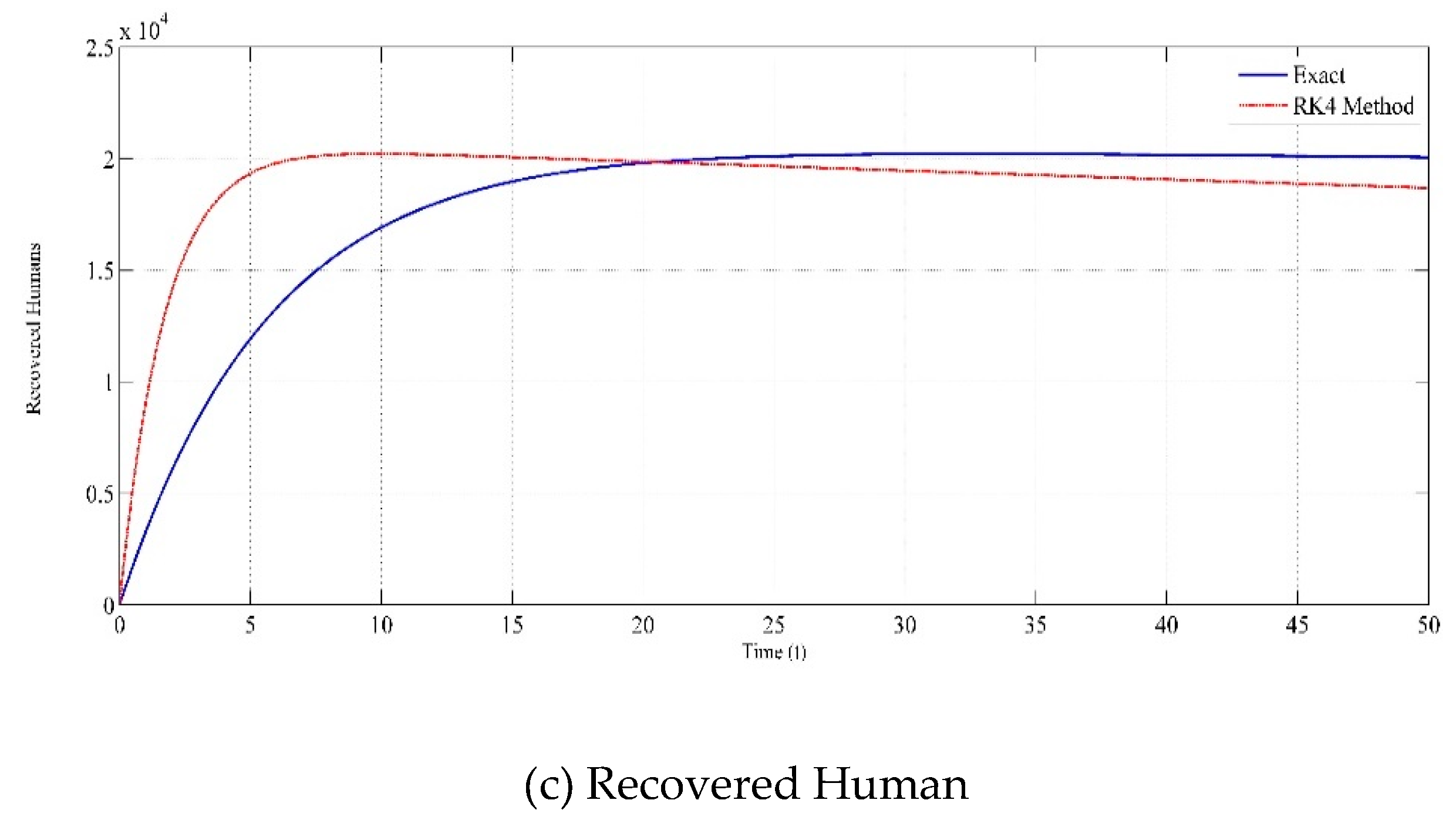
Figure 6.
Solution of Dengue dynamics using (a) Exact, (b) Euler, (c) RK4 Method and (d) No. of dengue cases reported in Dhaka city, Bangladesh from January to December in 2024.
Figure 6.
Solution of Dengue dynamics using (a) Exact, (b) Euler, (c) RK4 Method and (d) No. of dengue cases reported in Dhaka city, Bangladesh from January to December in 2024.
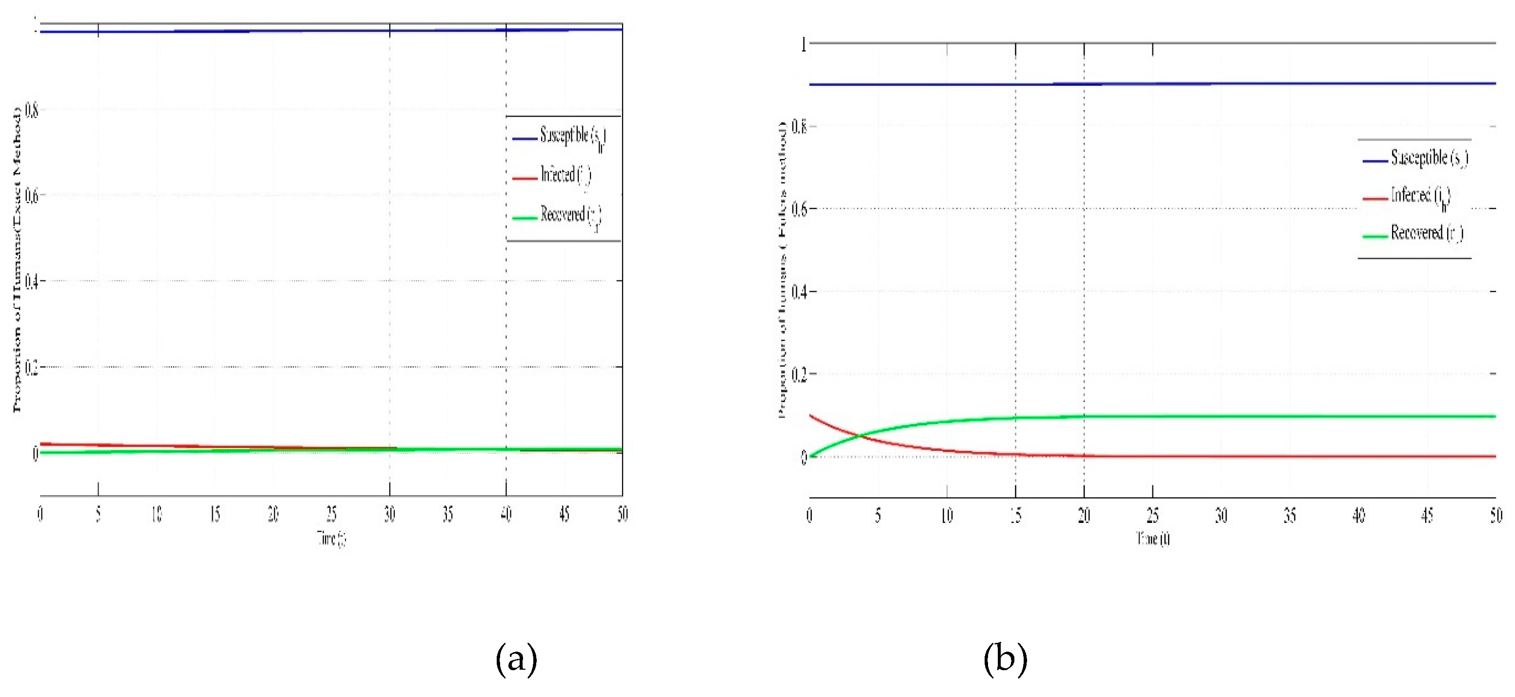
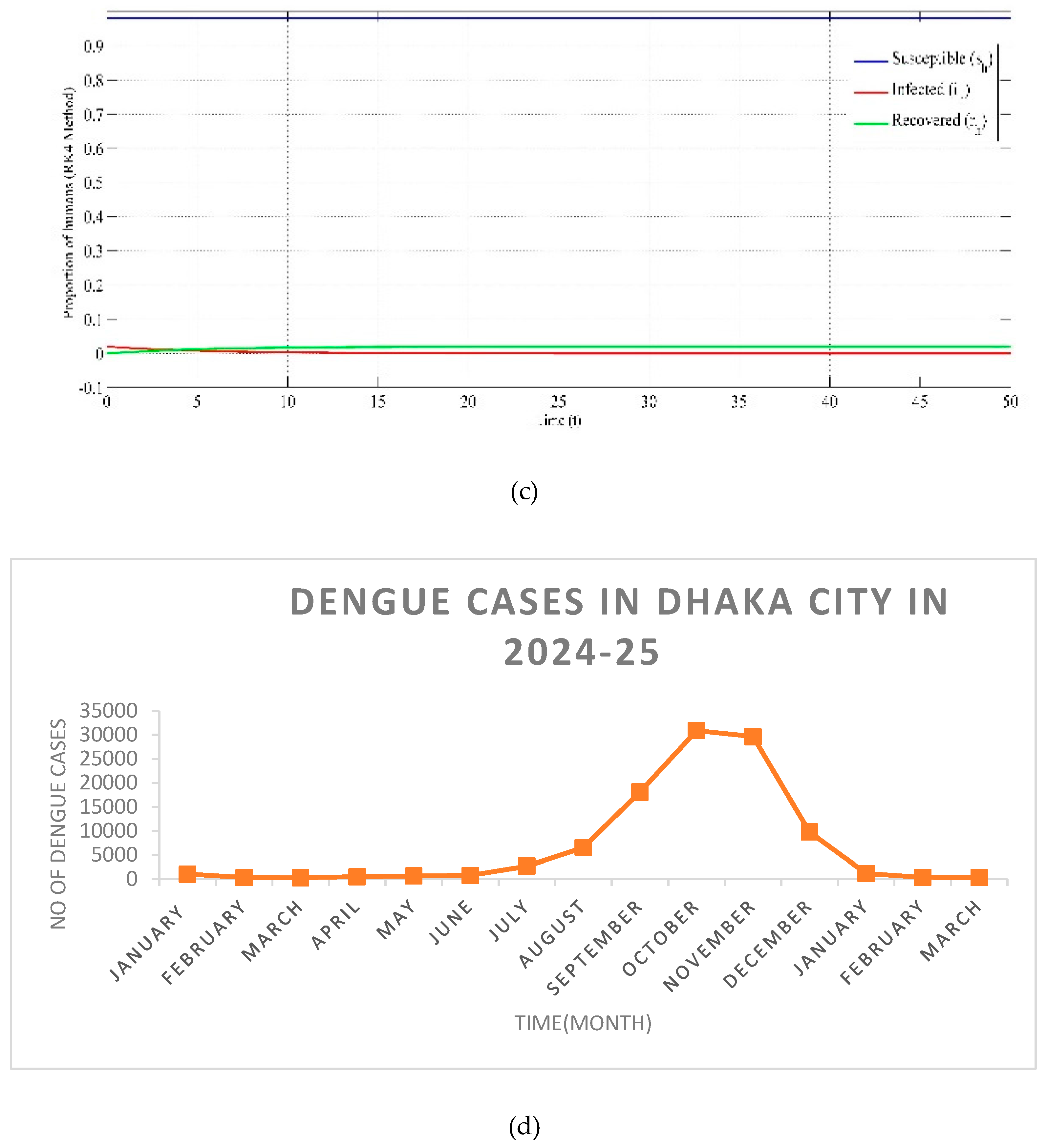

Table 1.
Parameters for Dhaka city.
| Parameters name | Symbols | Values |
| birth/death ratio in the human of the host | ||
| Recruitment rate of vector | 250,000 | |
| Transmission probability from vector to host | ||
| Transmission probability from host to vector | ||
| Recovery rate in the host human | ||
| biting rate of vector | ||
| Number of human size | 19578000 | |
| mortality rate in the human of vectors |
Disclaimer/Publisher’s Note: The statements, opinions and data contained in all publications are solely those of the individual author(s) and contributor(s) and not of MDPI and/or the editor(s). MDPI and/or the editor(s) disclaim responsibility for any injury to people or property resulting from any ideas, methods, instructions or products referred to in the content. |
© 2026 by the authors. Licensee MDPI, Basel, Switzerland. This article is an open access article distributed under the terms and conditions of the Creative Commons Attribution (CC BY) license.
Copyright: This open access article is published under a Creative Commons CC BY 4.0 license, which permit the free download, distribution, and reuse, provided that the author and preprint are cited in any reuse.


