

Submitted:
22 June 2026
Posted:
24 June 2026
You are already at the latest version
Abstract
A novel type of endogenous convex transformations of probability distributions is proposed for the controlled modification of a principal aggregate parameter while automatically preserving the properties of a probability distribution. Unlike conventional weighted distributions and mixture models, where the transformation mechanism is specified externally, the proposed approach determines the direction of evolution endogenously from the current distribution through a chosen outcome function and its associated principal moment. The resulting operator is constructed as a convex combination of the original density and its normalized weighted counterpart, ensuring non-negativity and unit normalization for all admissible transformation parameters. Analytical expressions describing the evolution of the principal moment are obtained, and the continuous limit of infinitely small transformations is investigated. An exact solution of the corresponding evolution equation is derived, showing that the continuous dynamics remains within the exponential family generated by the initial distribution and the outcome function. The gamma distribution is studied as a representative example. Explicit formulas are obtained for both finite and continuous gamma transformations. It is shown that repeated finite transformations naturally generate increasingly complex mixtures of gamma distributions, whereas the continuous dynamics preserves the gamma family by changing only its scale parameter. These results reveal a fundamental structural dichotomy between discrete mixture-generating transformations and continuous exponentially closed evolution.
Keywords:
endogenous transformations of distributions
; convex transformations
; weighted distributions
; mixtures of distributions
; exponential families
; gamma distribution
1. Introduction
Probability distributions are one of the basic tools for the mathematical description of random processes and mass phenomena. They allow not only to record the empirical variability of observed quantities, but also to define a compact analytical model of the system under study through the distribution function, moments, and shape parameters. In classical probability theory, distributions are considered the main language for describing random variables, their transformations, sums, limiting modes, and asymptotic regularities [1]. In applied statistics, the choice of distribution is associated with the nature of the data, the domain of definition of the random variable, the nature of asymmetry, the behavior of the tails, and the possibility of statistical estimation of the parameters [2,3]. In educational and applied literature, probabilistic models are also considered as the basis for the analysis of random processes, testing statistical hypotheses, parametric modeling, and forecasting in economic and technical problems [4,5,6]. In economic and mathematical applications, distributions are used to describe income, wealth, firm size, insurance claims, process durations, productivity, demand, and other positive or significantly asymmetric indicators. Kleiber and Kotz's monograph is specifically devoted to statistical distributions of sizes in economics and actuarial mathematics; it is emphasized that the normal distribution often poorly reflects the right-hand skewness and heavy tails of economic quantities, thus requiring special families of distributions, including gamma, lognormal, Pareto-like, and generalized models [7]. Work on the parametric representation of the upper part of income distributions also shows that the choice of a distribution family affects the assessment of inequality, the restoration of tails, and the interpretation of economic structure [8]. Consequently, the question of how a distribution can change when its aggregate characteristics are deliberately shifted has not only theoretical but also applied significance.
Among continuous distributions, the gamma distribution occupies a special place. It is defined on the positive semiaxis and is therefore naturally applied to quantities that cannot take negative values: waiting times, process durations, demand, payout sizes, flow rates, inventories, and insurance losses. Its density has the form
where k > 0 is the shape parameter, θ>0 is the scale parameter, Γ(k) is the gamma function.
The flexibility of the gamma family is due to the fact that changing the shape parameter allows one to describe a wide range of asymmetric positive distributions, and changing the scale controls the stretching of the distribution along the x-axis. The generalization of the gamma distribution proposed by Stacy expanded this class and strengthened its role as a universal family for modeling positive random variables [9]. In inventory management, gamma models are used to describe demand and lead times, since such quantities are positive and often have a pronounced right asymmetry; this is evident both in the early work of Burgin and in modern research by Tyworth [10,11]. In actuarial mathematics, gamma distributions are used in modeling insurance payments and claims [12], and in duration analysis they are one of the natural alternatives to exponential and Weibull time-to-event models [13].
Along with the problem of selecting a distribution, a more general question arises: how to transform a given distribution so as to preserve its probabilistic correctness but controllably change some aggregate indicator. Such an indicator could be understood as mathematical expectation, average performance, productivity, utility, profitability, or another state function. In general, such an indicator can be written as
where g(x) defines a meaningful characteristic of the state. In applied problems, such a transformation can be interpreted as a redistribution of mass between efficiency classes, strengthening of more effective states, a shift in the structure toward higher indicator values, or modeling of selection.
One of the closest approaches to this approach is the theory of weighted distributions. Its origins are linked to Rao's work on discrete distributions arising from ascertainment methods, i.e., observation procedures in which the probability of an object being included in a sample depends on its characteristics [14]. Patil and Rao developed this idea in a general theory of weighted distributions and size-biased sampling [15]. In standard form, a weighted distribution is given by the formula
where w(x)≥0 is the weighting function. Choosing w(x)=x yields a size-biased distribution, i.e., a distribution in which objects with larger x values have an increased probability of being observed.
Modern reviews of weighted distributions show that this construct has a wide range of applications and serves as a general mathematical framework for describing biased samples and reweighted probability models [16]. However, in the classical theory of weighted distributions, the weighting function is usually specified externally. The researcher determines in advance which characteristic should enhance or weaken the probability of a state, after which the normalized distribution f w is constructed . Such reweighting is a powerful tool, but in itself it does not specify an intermediate controlled transition from the original distribution to the reweighted one and does not consider how the change in the principal moment is related to the geometry of the distribution trajectory.
Another closely related class of models is formed by finite mixtures of distributions. In the classical setting, a mixture is written as
where f i (x) are the components of the mixture, and π i are their weights.
Such models are widely used to describe heterogeneous populations and multimodal data. Nielsen and Nock consider finite convex combinations of given distribution components in the context of w-mixtures and mixture geometry [17]. Mixtures of gamma distributions play a special role, being used to model complex positive data, clustering, and statistical inference—the corresponding methodology is discussed in detail in the work of Young et al. [18]. However, here too, the mixture components are typically assumed to be given as model elements, and the task consists of estimating the weights, parameters, and number of components. In other words, the mixture is introduced as a statistical structure.
In continuous models of probability mass redistribution, replicator dynamics is a natural analogue. In the discrete case, it is often written as
where x i is the proportion of a state or type, f i is its fitness, and is the average fitness of the population. Modern reviews of replicator dynamics show that such equations are used in game theory, evolutionary models, selection dynamics, and adaptive systems [19]. In essence, this construction is close to distribution transformations in which states with above-average performance are strengthened, while states with below-average performance are weakened. However, even in replicator dynamics, the fitness function is, in most settings, specified externally: the model determines in advance which states are more advantageous or fitter.
Thus, the approaches discussed—weighted distributions, size-biased transformations, finite mixtures, gamma mixtures, and replicator dynamics—form an important theoretical backdrop for the problem of controlled distribution transformation. However, they share a common methodological feature: the key elements of the transformation are usually specified a priori. In weighted distributions, the weighting function w(x) is chosen in advance; in size-biased transformations, the reweighting rule is fixed; in mixture models, the mixture components are assumed in advance; in gamma mixtures, the gamma components are considered as the selected class of the statistical model; in replicator dynamics, the fitness function is specified; and in exponential families, the parametric structure is fixed in advance. In all these cases, the distribution transformation is largely determined by the external choices of the researcher.
This paper takes a different approach. It proposes to consider the distribution transformation as an endogenous, moment-controlled process in which the direction of change is not specified by a model, as in [14,15,16,17,18,19], but is determined by the current distribution itself and the selected outcome function.
Moreover, the transformation must automatically preserve the properties of the original distribution, such as non-negativity and normalization. Geometrically, this means moving along a segment within a convex set of probability distributions. Thus, the desired transformation operator is naturally related to mixture geometry but differs from classical mixtures in that the target component is not predetermined, but is generated by the original density itself.
The gamma distribution is chosen as a basic example: it simultaneously has broad practical significance [9,10,11,12,13,14,15] and allows for an analytically transparent demonstration of the methods and capabilities of endogenous, convex transformations
Thus, the goal of this paper is to construct and study a class of endogenous convex transformations of distribution functions. The paper links weighted distributions, size-biased transformations, mixture geometry, gamma mixtures, replicator dynamics, and exponential geometry in a single operational framework, but shifts the emphasis from externally imposed models to the endogenous mechanism of distribution transformations.
2. Methodology
It is necessary to formalize the space of distributions under consideration, determine the main aggregate parameter characterizing the average performance of the system, and introduce an operator that ensures controlled variation of this parameter while automatically maintaining the probabilistic correctness of the transformed distribution. Next, the corresponding definitions are formulated, the basic properties of the constructed operator are proven, and its relationship with continuous limit dynamics is explored. Particular attention is given to the geometric interpretation of the transformation as a motion in a convex set of probability distributions.
Problem Statement and Transformation Operator
Given a probability space (Ω, F, µ), where µ is the base measure, let σ(x) be the original probability density of P with respect to µ, that is,
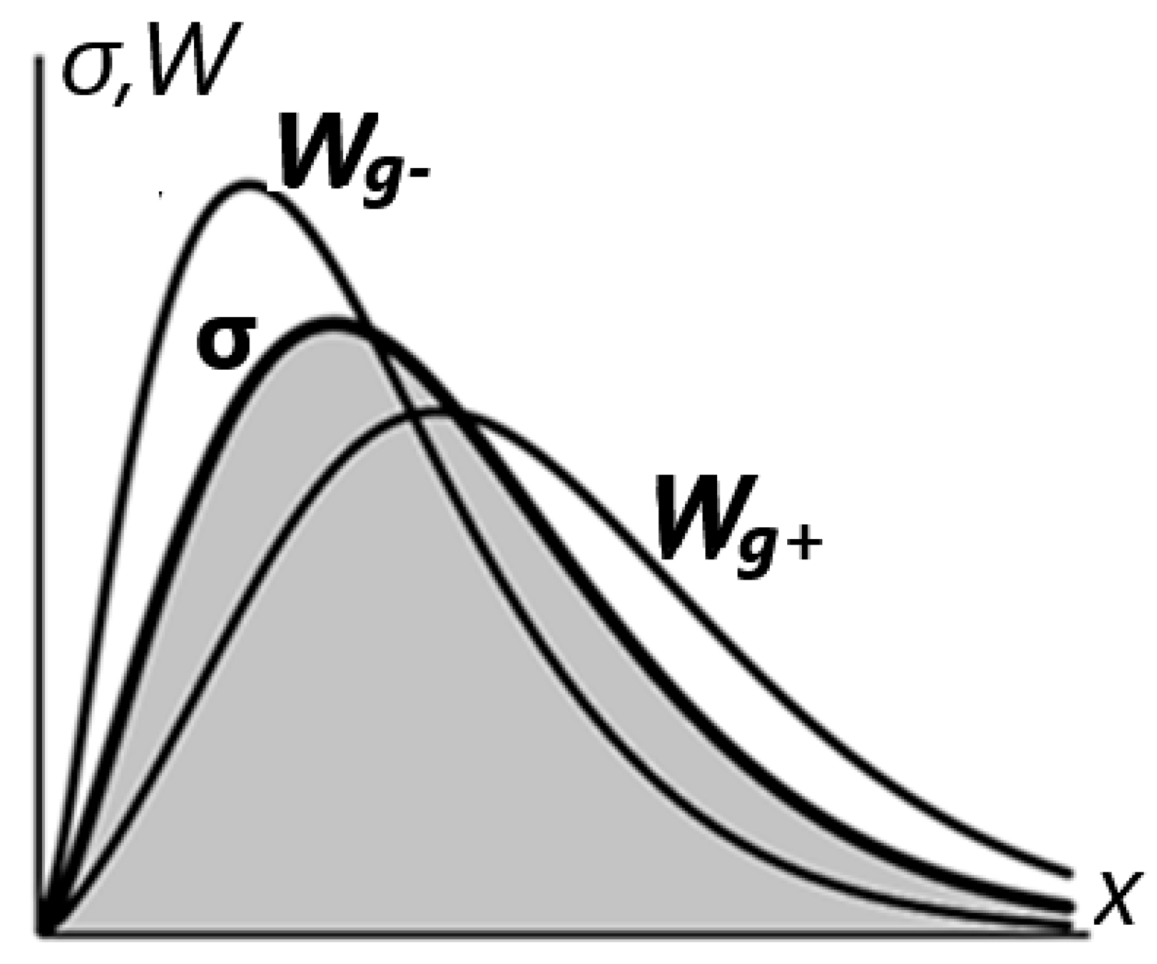
It is represented by the center line σ(x) in Fig. 1. According to the normalization condition (1), the area under this curve is equal to unity.
The initial density σ(x) describes the distribution of the "mass" (state probability) over states x. The function g(x) defines the "effectiveness" ("utility", "output", "profitability", "efficiency") of a state.
A non-negative result function is specified
and the main aggregate parameter (average performance) is determined
Associated normalized g-weighted density
where p is the principal moment according to (), determined under the condition 0 < p < ∞.
Since the normalization condition is met:
then, therefore, is the correct probability density function. It is a normalized transformation operator that enhances those regions where g(x )>p and weakens those where g(x)<p. This effect is clearly shown in Fig. 1: the lower curve represents the weighted density in the case where the weighting function g ( x ) is increasing (e.g., g ( x )= x ), and the upper curve in the case of decreasing performance (e.g., g ( x )=1/x ).
Figure 1.
The type of probability density curves: σ is the initial density, and are the weighted densities, respectively, with
increasing and decreasing performance functions g.
Figure 1.
The type of probability density curves: σ is the initial density, and are the weighted densities, respectively, with
increasing and decreasing performance functions g.
A simple additive transformation of the distribution is
where R is the distribution function correction. However, this transformation raises significant issues: the need to check for non-negativity and special measures to ensure normalization. Furthermore, the geometric interpretation of the transformation is not sufficiently clear.
Convex transformation operator.
eliminates these difficulties automatically: non-negativity and normalization to unity are preserved, the transformation occurs in a convex set of admissible distributions
in this case, the magnitude of the change is controlled by one parameter α. The point σ belongs to ∆, the point W g [σ] also belongs to ∆. Therefore, the entire segment
also lies in ∆.
The main operator is considered
provided that 0 ≤ α ≤ 1. An equivalent representation of the operator
The geometric meaning of the transformation is that it can be interpreted as a transformation from the original distribution σ in the direction of the g-resulting distribution W g [σ].
Basic Properties of the Operator
Let g ≥ 0, 0 < p < ∞, 0 ≤ α ≤ 1. Then, since
σ(x) ≥ 0 and W g [σ](x) ≥ 0, then [σ](x) ≥ 0. The integral is equal to
therefore, [σ] is the correct normalized density. For the main parameter m g of this distribution, we obtain
By the Cauchy–Bunyakovsky inequality
hence,
Since g is usually not a constant, this inequality is strict, and for α > 0 the main parameter increases. As a consequence, when setting the target value p* and satisfying the admissibility condition
the parameter α is determined
The relation shows that the convex operator allows one to analytically obtain a given target value of the principal moment of the distribution.
Transition to Continuous Time
The integral transformation of distributions is considered as the limiting regime of a sequence of infinitesimal steps. Let α = ε, where ε is small. Then
or
If we interpret ε as a time step dt , then we obtain a limit transition
where
The natural continuous limit according to () is the equation
Basic Properties of Continuous Dynamics
1) Maintaining the standard
If we take the ratio as a basis
then substitution (23) will give
The derivative of the total mass is zero, therefore
If at the initial moment
then in all subsequent moments as well
that is, the normalization is preserved.
Thus, positive and negative local changes in density are mutually compensated so that the total probability mass is preserved and only its redistribution between states occurs.
2) Evolution of the main parameter
If p ( t ) is determined by expression (22), then
Substitution (23) gives
Hence,
Since g is not a constant, the right-hand side is non-negative. In the special case of g(x) = x
and therefore
Taking into account
it turns out
That is, if there is a spread, then an increase in the average is observed, but if the distribution degenerates (tends to a delta function), the growth stops.
Exact Solution of Continuous Dynamics
Let σ(x, t) satisfy equation (37), where p ( t ) is defined according to (36).
Then the solution of the equation has the form
where σ 0 (x) = σ( x, 0), and λ(t) is determined by the equation
The result is checked by differentiating the solution ( 35). Substitution is made
where
Then
Differentiating with respect to t gives:
But
That's why
Hence,
If you put
then we get equation (23), which is what needed to be proven.
Thus, we can draw a conceptual conclusion: the continuous dynamics always remains within the exponential family generated by the initial density σ 0 and the result function g. In other words, the entire solution is obtained by the exponential slope of the initial density, and the evolution is reduced to a change in a single parameter λ(t). More precisely, the set
is the minimal natural class in which the solution resides. This is the main difference from the finite case: the finite operator tends toward mixtures, while continuous dynamics tends toward exponential tilt.
3. Results
The gamma distribution was chosen as the object for implementing the transformation methods. It is one of the most widely used continuous distributions in statistics, reliability theory, economics, actuarial calculations, and waiting time analysis. Furthermore, for the outcome function g(x)=x, its g-weighted transformation has a fairly simple analytical form: thus, the gamma distribution serves as a visual and mathematically transparent illustration of the identified transformation properties of distributions, both finite and continuous.
Final Gamma Transformation
Let us consider the most illustrative special situation. Let x ≥ 0, g(x) = x, and the original density be a gamma distribution.
Then the first moment (mathematical expectation)
The operator for the gamma distribution takes the form
Substitution (46) yields
Next, the substitution of identity
gives
Hence,
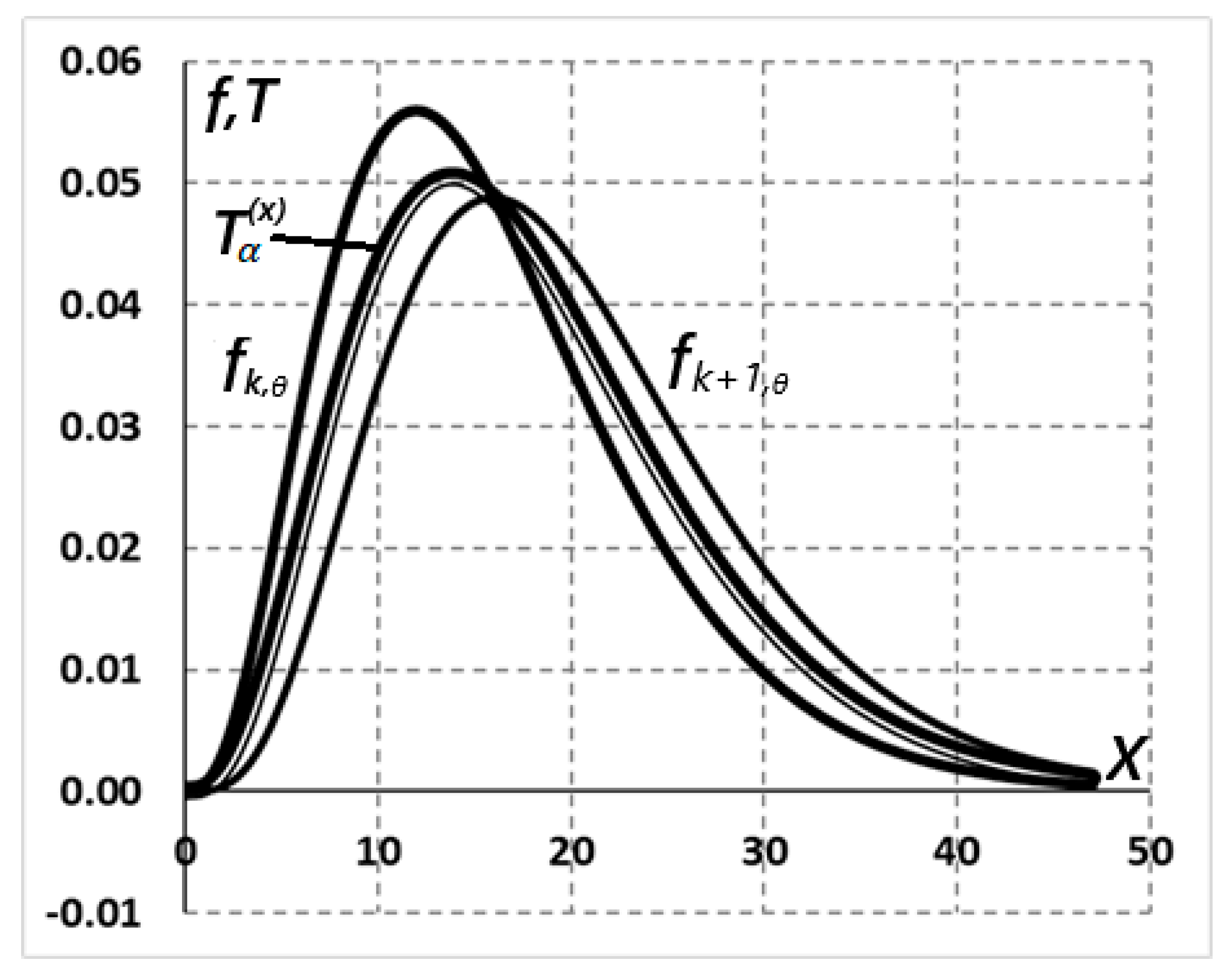
It turns out that the final operator yields not a gamma distribution proper, but a weighted mixture of two gamma distributions of adjacent orders. Transformation (52) is shown in Fig. 2: the upper curve represents the initial distribution f k ,θ , the lower curve represents f k +1,θ , and the middle curve represents the weighted mixture .
Figure 2.
The final operation of transforming the distribution into a binary mixture: curves f k ,θ and f k +1,θ are the initial and final distributions, – suspended mixture, parameters k=4, θ=4, α=0.5.
Figure 2.
The final operation of transforming the distribution into a binary mixture: curves f k ,θ and f k +1,θ are the initial and final distributions, – suspended mixture, parameters k=4, θ=4, α=0.5.
Finite Operator Iterations and Complexity Growth
A sequence of finite transformations is considered
σ 0 = f k ,θ
For the result function g(x)=x, each iteration preserves the representation as a mixture of gamma distributions:
The initial condition is
If you enter the value
representing the dimensionless principal moment of the current mixture, then its g-weighted transform will be written as
where the mixture coefficients satisfy the recurrence relation
under boundary conditions
This recursive method completely determines each iteration. Thus, repeated applications of the finite operator preserve the distribution's representation as a finite mixture of gamma densities with successive parameters of the form k, k+1,…, k+n, while simultaneously increasing the number of its components. Consequently, the finite operator possesses a natural mixture-generating property, and its successive applications lead to an increase in the distribution's structural complexity.
Figure 3 shows the results of calculating three successive iterations of the finite operator with the initial gamma distribution σ 0 = f k, θ .
Gamma Transform in Continuous Time
If we return to the gamma density (46), then for g(x) = x the theorem on the exact solution gives
Only the coefficient of x in the exponent changes, which is equivalent to a change in the scale parameter. After renormalization, the distribution function takes the form
where
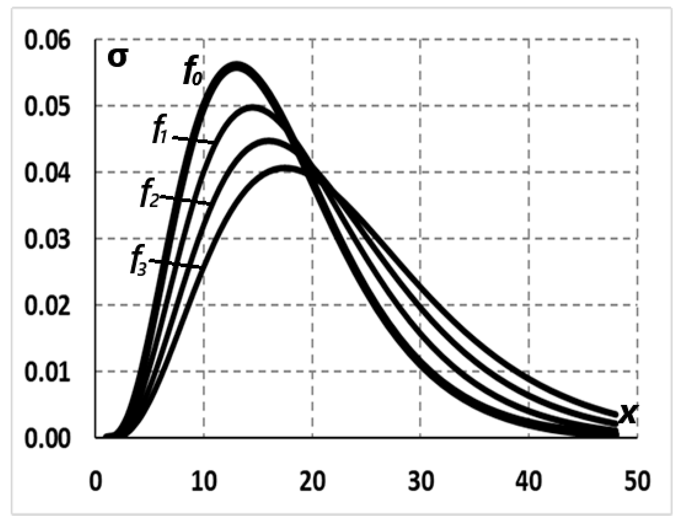
Thus, in the continuous mode, the gamma distribution is not transformed into a mixture, but remains within the gamma family with the same shape parameter k and a changing scale parameter θ(t).
Figure 4 shows a continuous transformation of the initial gamma distribution f 0 = f ( x , 0) through intermediate densities f 1 , f 2 to the current distribution f 3 = f ( x , t ).
Thus, the fundamental difference between the finite and continuous transformation modes is that for the same torque-controlled transformation mechanism:
- the discrete final step has a mixture-generating character;
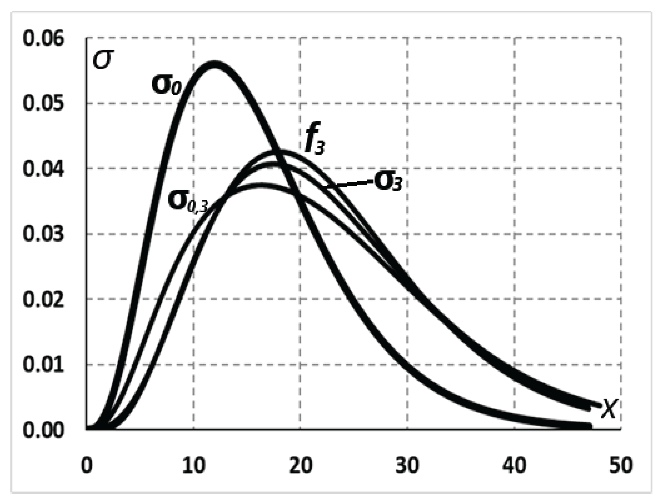
- the continuous limit d σ/dt = σ (g/p − 1) has an exponentially closed character. In other words, discrete dynamics naturally leads to mixtures, and continuous dynamics to exponential families. The reason is that the final step uses a linear factor 1+ α (g/p-1) which, when infinitely small steps accumulate, turns into an exponential of the form As in the classical comparison of an arc and its subtending chord, the final linear step and the limit of the set of small steps do not coincide. This effect is visible in Fig. 5: three comparable transformations of the initial density σ 0 are presented - three successive single steps - σ 3 , an equivalent single-step transformation - σ 0.3 , and an equivalent continuous transformation - f 3 . All three finite distributions are characterized by the same principal moment p .
When comparing finite and continuous modes, one might intuitively expect that a finite change in the principal parameter should lead to the same result as a continuous transformation. However, a discrete step yields a linear slope, while continuous dynamics yields an exponential slope. This explains the discrepancy in results. From a theoretical perspective, the general theorem on the exponential form of a continuous solution is central. The gamma case is important as a clear consequence: it demonstrates how discrete and continuous modes can differ radically within the same family.
Figure 5.
Comparison of the results of finite and continuous transformations: σ 0 is the initial gamma density ( p 0 = 16), σ 3 is three unit steps, σ 0.3 – one triple step ( α = 0.5), f 3 – continuous equivalent transformation ( α = 0.525), final moment p = 22.3.
Figure 5.
Comparison of the results of finite and continuous transformations: σ 0 is the initial gamma density ( p 0 = 16), σ 3 is three unit steps, σ 0.3 – one triple step ( α = 0.5), f 3 – continuous equivalent transformation ( α = 0.525), final moment p = 22.3.
4. Interpretation
The results obtained allow us to take a fresh look at the problem of controlled transformation of probability distributions. Their primary significance lies not so much in the construction of yet another class of operators, but rather in identifying two fundamental properties of the proposed scheme: its endogenous nature and the existence of a fundamental dichotomy between discrete and continuous transformation modes.
In most existing approaches, the distribution transformation rule is specified externally. In weighted distributions, a weighting function is preselected, determining the reweighting mechanism. In size-biased transformations, a rule for strengthening individual states is fixed. In finite mixture models, the composition of the components is assumed to be known, after which their weights and parameters are estimated. In replicator dynamics, the fitness function is also considered an externally specified characteristic of the system.
The approach proposed in this paper is based on a different methodology. The direction of the transformation is determined not by an external model hypothesis, but by the current distribution structure itself, through its main aggregate parameter and the selected outcome function. In other words, the operator is constructed endogenously: its action is entirely determined by the internal characteristics of the distribution being transformed.
It is precisely this circumstance that fundamentally distinguishes the proposed construction from known reweighting operators. Thus, the convex transformation acquires a natural interpretation as an internal redistribution of probability mass between states without invoking external structural assumptions.
The final transformation is implemented as a movement along a segment between two valid probability distributions. Therefore, the entire trajectory automatically belongs to the convex set of admissible distributions. Unlike additive schemes, there is no need for additional non-negativity and normalization checks.
A significant result of the work is the structural dichotomy between finite and continuous transformation modes. The discrete operator has a linear convex nature and, when applied successively, generates increasingly complex mixtures of distributions. Even for the gamma distribution, the first step leads to a binary mixture of adjacent orders, and subsequent iterations successively increase the number of components.
Taking the continuous limit leads to a qualitatively different picture. The resulting evolution equation admits an exact solution in the form of an exponential slope of the initial density, so that the entire dynamics remains within an exponential family that includes both the initial density and the resulting function.
Thus, the same moment-controlled mechanism, depending on the implementation method, leads to fundamentally different mathematical structures: the discrete mode naturally gravitates to the geometry of mixtures, while the continuous mode gravitates toward the geometry of exponential families.
Taken together, the obtained results allow us to formulate the following provisions that determine the scientific novelty of the work.
1) A new type of endogenous convex transformations of probability distributions is proposed, in which the direction of transformation is determined by the internal characteristics of the distribution itself, and is not specified by an external model construction.
2) It is shown that finite mixtures can arise as an analytical consequence of the action of such an operator, and not as an a priori postulated statistical class.
3) A dichotomy is established between discrete and continuous implementations of a single moment-controlled mechanism: discrete dynamics have a mixture-generating character, while continuous dynamics retain exponential closure and remain within the exponential family generated by the original distribution density.
5. Conclusions
This paper proposes a new type of endogenous convex transformation of distribution functions based on controlled variation of the principal aggregate parameter via an internally defined operator mechanism. Unlike traditional approaches that use externally imposed reweighting rules or pre-determined mixture components, the direction of the transformation in the proposed scheme is determined by the current distribution itself via the outcome function and the corresponding principal moment.
The constructed operator automatically preserves the fundamental properties of the probability distribution, including non-negativity and normalization, while changes to the main aggregate parameter allow for analytical control. This provides a constructive basis for constructing controlled transformations of distributions without compromising their probabilistic correctness.
The main theoretical result is the establishment of a structural dichotomy between finite and continuous modes of action of the same operator mechanism. Finite transformations naturally generate families of mixtures, whereas continuous limit dynamics preserves the exponential structure and remains within the exponential family generated by the original distribution density. Discrete and continuous realizations of the redistribution of the probability mass have qualitatively different geometries.
A study of the gamma distribution confirms the general theoretical conclusions and provides a clear analytical interpretation. It was found that in the finite regime, the operator consistently generates mixtures of gamma distributions of adjacent orders, while in the continuous regime, membership in the gamma family is maintained even when the scale parameter changes. This example demonstrates that the identified dichotomy is not an abstract theoretical effect, but manifests itself in one of the most widespread and practically significant classes of distributions.
The results obtained allow us to consider the proposed approach as a basis for further development of a general theory of endogenous transformations of probability distributions. Research into broader classes of result functions, multivariate distributions, and nonlinear transformation operators, as well as the study of stationary regimes and asymptotic properties of the corresponding dynamic systems, appears promising.
From an applied perspective, the use of the developed operator apparatus is relevant for modeling structural redistribution processes in economic, biological, social, and technical systems, where the evolution of distributions is determined by the internal characteristics of the objects of study themselves. A separate promising direction is the study of the combined effect of the proposed endogenous transformations with diffusion, stochastic, and optimization mechanisms, as well as their relationship to distribution control problems and information geometry.
From a broader methodological perspective, the obtained results demonstrate that convex transformations, operator endogeneity, and the dichotomy between discrete and continuous dynamics can be viewed as interrelated elements of a unified concept of the evolution of probability distributions. This opens new possibilities for integrating weighted distributions, mixture geometry, exponential families, and moment-controlled dynamics within a unified operator framework.
Financing
This research received no external funding.
Statement of the Ethics Committee
Unsuitable.
Informed Consent Statement
Unsuitable.
Data Accessibility Statement
The calculated data presented in this study are available upon request from the author.
Conflicts of interest
The author declares that he has no conflict of interest.
References
- Feller, W. An introduction to probability theory and its applications (Vols. 1–2); John Wiley & Sons, 1968–1971; Available online: https://archive.org/details/dli.ernet.5666/page/11/mode/2up.
- Johnson, N.L.; Kotz, S.; Balakrishnan, N. Continuous Univariate Distributions; J. Wiley & Sons, New York, 1994; Volume 2, Available online: https://www.wiley.com/en-us/shop/general-introductory-statistics/continuous-univariate-distributions-volume-1-2nd-edition-p-9780471584957.
- Evans, M. Hastings, N. & Peacock, B. Statistical distributions (2nd Edition); John Wiley: New, 1993; p. 170 pages. ISBN 0-471-55951. [CrossRef]
- Chernova, N. I. Teoriya veroyatnostey. Uchebnoye posobiye dlya studentov ekonomicheskikh spetsial'nostey NGU [Probability Theory. A textbook for students majoring in economics at NSU]. 2007. Available online: https://tvims.nsu.ru/chernova/tv/portr.pdf?utm_source=chatgpt.com.
- Tyurin, Y.U.N.; Makarov, A.A. Analiz dannykh na komp'yutere. Izd. 3"ye, pererab. i dop./[Data analysis on a computer. 3rd edition, revised and enlarged] Pod red. V. E. Figurnova — M.: INFRA–M, — 528 s; 2002; Available online: https://www.hse.ru/data/2015/01/15/1107271356/%D0%9C%D0%B0%D0%BA%D0%B0%D1%80%D0%BE%D0%B2%20%D0%90.%D0%90._BOOK.pdf?utm_source=chatgpt.com.
- Bure, V. M.; Parilina, Ye. M. Teoriya veroyatnostey i matematicheskaya statistika. In Probability Theory and Mathematical Statistics] Izdatel'stvo «Lan'»; 2013; Available online: https://reader.lanbook.com/book/505410?demoKey=8d0f429f74d49a528142701943f7a62f#2.
- Kleiber, C.; Kotz, S. Statistical Size Distributions in Economics and Actuarial Sciences; Wiley, 2003. [Google Scholar] [CrossRef]
- Hlasny, V. Parametric Representation of the Top of Income Distributions: Options, Historical Evidence and Model Selection. In Working Papers 547, ECINEQ, Society for the Study of Economic Inequality; 2020. [Google Scholar] [CrossRef]
- Stacy, E. W. A Generalization of the Gamma Distribution. Ann. Math. Stat. 1962, 33(3), 1187–1192. [Google Scholar] [CrossRef]
- Tyworth, J. E. The Gamma Distribution and Inventory Control: Disruptive Lead Times Under Conventional and Nonclassical Conditions. Logist. MDPI 2025, vol. 9(2), pages 1–23. [Google Scholar] [CrossRef]
- Burgin, T.A. The Gamma Distribution and Inventory Control. In Operational Research Quarterly (1970-1977); Published By; Palgrave Publishers Content source, 1975; Vol. 26, No. 3, Part 1, pp. 507–525. [Google Scholar] [CrossRef]
- Embrechts, P. S. A.; Klugman, H. H. Panjer and G. E. Willmot: Loss Models: From Data to Decisions. In ASTIN Bulletin; Wiley, New York, 1998; Volume 28, 1, pp. 163–164. [Google Scholar] [CrossRef]
- Cox, D. R.; Oakes, D. Analysis of Survival Data; Chapman and Hall: London–New York, 1984. [Google Scholar] [CrossRef]
- Rao, C. R. On Discrete Distributions Arising out of Methods of Ascertainment. Sankhyā Indian J. Stat. Ser. A (1961-2002) 1965, 27(2/4), 311–324. Available online: http://www.jstor.org/stable/25049375.
- Patil, G. P.; Rao, C. R. Weighted distributions and size biased sampling with applications to wildlife populations and human families. Biometrics 1978, 34, 179–189. [Google Scholar] [CrossRef]
- Pyne, S. On Weighted Distributions and Applications. In Special Proceedings of the 22nd Annual Conference of the Society of Statistics, Computer and Applications (SSCA); 2020; pp. 153–162. [Google Scholar] [CrossRef]
- Nielsen, F.; Nock, R. On w-mixtures: Finite convex combinations of prescribed component distributions. abs/1708.00568; ArXiv. 2017. Available online: https://www.semanticscholar.org/paper/On-w-mixtures%3A-Finite-convex-combinations-of-Nielsen-Nock/d374ddf5b7a451e6438bcd77bcd1f0c255e1a58e.
- Young, D.S.; Chen, X.; Hewage, D.C.; et al. Finite mixture-of-gamma distributions: estimation, inference, and model-based clustering. Int. Fed. Classif. Soc. (IFCS) 2019, V 13(4), 1053–1082. [Google Scholar] [CrossRef]
- Sylvain, S. Replicator dynamics: Old and new. J. Dyn. Games 2020, 7(4), 365–386. [Google Scholar] [CrossRef]
Figure 3.
Iterations of the finite operator generating mixtures gamma distribution mixtures: σ 0 – initial gamma density, k =4, θ=4; σ 1 , σ 2 , σ 3 – iteratively transformed mixtures, α=0.5;.
Figure 3.
Iterations of the finite operator generating mixtures gamma distribution mixtures: σ 0 – initial gamma density, k =4, θ=4; σ 1 , σ 2 , σ 3 – iteratively transformed mixtures, α=0.5;.
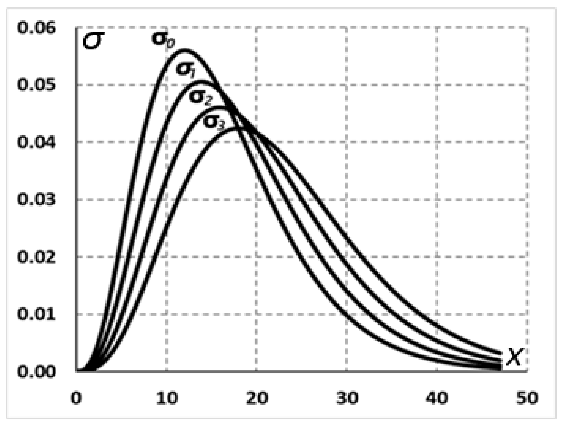
Figure 4.
Continuous transformation of the distribution function: sequence of gamma distributions f 0 , f 1 , f 2 , f 3 with parameters forms θ, respectively – 4.0; 4.5; 5.0; 5.5, parameter k =4.
Figure 4.
Continuous transformation of the distribution function: sequence of gamma distributions f 0 , f 1 , f 2 , f 3 with parameters forms θ, respectively – 4.0; 4.5; 5.0; 5.5, parameter k =4.
Disclaimer/Publisher’s Note: The statements, opinions and data contained in all publications are solely those of the individual author(s) and contributor(s) and not of MDPI and/or the editor(s). MDPI and/or the editor(s) disclaim responsibility for any injury to people or property resulting from any ideas, methods, instructions or products referred to in the content. |
© 2026 by the authors. Licensee MDPI, Basel, Switzerland. This article is an open access article distributed under the terms and conditions of the Creative Commons Attribution (CC BY) license (http://creativecommons.org/licenses/by/4.0/).
Copyright: This open access article is published under a Creative Commons CC BY 4.0 license, which permit the free download, distribution, and reuse, provided that the author and preprint are cited in any reuse.


