

Submitted:
30 June 2026
Posted:
02 July 2026
You are already at the latest version
Abstract
We construct a k-shadow complex Δk(N) from the nerve N of a convex sensor cover and prove that the region covered by at least k sensors is homotopy equivalent to Δk(N), recovering the usual nerve-based coverage test at k = 1. We test the construction on five independent synthetic sensor fields. Two confirm exact agreement with direct geometric sampling. A third, an unstructured random field, exposes instability in the raster-based ground truth at near-tangent sensor contacts, which we trace to twenty disk pairs within 0.05 length units of tangency; the exact nerve classifies every one correctly. A fourth, a densely clustered field, shows that Δ2(N) itself can be far larger than its underlying sensor count suggests: removing an initial clique-size obstruction in the construction reveals an object with over 800,000 vertices, against under 500 for the other fields tested. All scripts, data, and logs are supplied for reproduction.
Keywords:
sensor networks
; nerve complex
; k-fold coverage
; simplicial homology
MSC: Primary 55U10; Secondary 55N31, 68R05, 90B18
1. Introduction
A sensor network is, for coverage purposes, a finite collection of regions , each the detection footprint of one node, and the basic question is whether their union covers some domain of interest. When node positions are unknown or unreliable, a remarkable fact makes this question tractable from connectivity data alone. Ghrist and Muhammad, and de Silva and Ghrist in subsequent work, showed that the topology of the union of the can be tested from the nerve of the cover, a purely combinatorial object recording which subsets of nodes have overlapping footprints, with no metric information beyond an overlap test [1,2,3]. The underlying tool is a theorem of Borsuk: the union of a cover by convex (or, more generally, contractible-intersection) sets is homotopy equivalent to the nerve of the cover [5]. A nontrivial first homology class in the nerve signals a hole in the coverage that no individual overlap test would reveal (see [8] for standard background on simplicial homology).
Ordinary coverage, meaning every point seen by at least one sensor, is often not what a deployment actually needs. Reliability against node failure, handover in cellular networks, and multi-static sensing all require k-fold coverage: every point of the domain seen by at least k distinct sensors, so that the loss of any nodes still leaves the domain covered [10]. The existing homological treatment of this problem, due to Vergne, Decreusefond, and Martins, works by an iterative reduction: k-coverage is interpreted as k disjoint layers of ordinary 1-coverage, found one at a time by a simplicial reduction algorithm [11,12]. This is effective, but it uses an auxiliary partitioning problem at each layer, and the partition is not unique.
We give a different, direct construction. From the ordinary nerve complex N of the cover, the same object already needed for 1-coverage checking, we build a derived complex , the k-shadow complex, whose vertices are the -dimensional faces of N and whose higher faces are read off directly from N’s own combinatorics, with no new geometric computation and no search for disjoint layers. We prove that the region of covered at least k times is homotopy equivalent to (Theorem 3), by a direct, two-line application of Borsuk’s nerve lemma to a secondary cover built from N’s own faces. For , , recovering the de Silva–Ghrist criterion exactly as a special case.
We check the construction computationally for and against an independently computed ground truth, and report a real implementation bug: a discretized intersection test that produced false negatives on thin, marginal overlaps, found through this cross-check and corrected with an exact closed-form test.1 We then extend the same check to four additional sensor fields with qualitatively different geometry, asking whether the original agreement on a single field reflects a property of the construction or an artifact of that one field.
The remainder of the paper is organized as follows. Section 2 fixes notation for the nerve complex and states the two classical theorems the construction rests on. Section 3 defines . Section 4 proves the main equivalence. Section 5 draws the homological corollary used for checking coverage. Section 6 reports the computational experiment, beginning with a single field and its implementation history (Section 6.1, Section 6.2 and Section 6.3) before extending to four further fields (Section 6.4, Section 6.5, Section 6.6 and Section 6.7). Section 7 positions the construction against the existing k-coverage literature. Section 8 records the construction’s limitations honestly, including the scaling limit diagnosed in Section 6.7. Section 9 concludes.
2. Preliminaries
Throughout, are closed convex regions (in particular, closed disks of a common radius, though nothing in this section uses equal radii).
Definition 1
(Nerve complex). The nerve N of the cover is the abstract simplicial complex on vertex set whose faces are exactly the subsets with .
Theorem 1
(Nerve Lemma; Borsuk 1948 [5]). If every nonempty finite intersection is contractible, then the union is homotopy equivalent to the geometric realization of the nerve N.
For convex sets in , every nonempty finite intersection is itself convex, hence contractible, so the Nerve Lemma always applies to a cover by convex regions; this is the classical Čech theorem used throughout the sensor-coverage literature [2,9].2
The second classical fact we use is computational rather than topological. It lets the entire nerve be recovered from its 2-skeleton (vertices, edges, and triangles) alone, without testing higher-order intersections directly.
Theorem 2
(Helly 1923 [6]). Let be convex sets in . If every 3 of them have a common point, then all m of them have a common point.
Corollary 1
(Two-skeleton determines the nerve). For a cover by convex sets in , a candidate vertex set σ with is a face of N if and only if every 3-element subset of σ is a face of N.
Proof.
If is a face, every subset of is a face, in particular every 3-element subset. If every 3-element subset of is a face, then every 3 of the convex sets share a common point, so by the Helly theorem all of them do, and is a face. □
We use Corollary 1 in Section 6 only as a computational shortcut: it never changes which sets are faces, it only changes how cheaply that fact can be verified.
3. The k-Shadow Complex
Fix . Write for the coverage multiplicity at a point , and .
Definition 2
(k-shadow complex). Let N be the nerve of and let denote the set of -dimensional faces of N (i.e. the k-element subsets with ). The k-shadow complex is the abstract simplicial complex with vertex set , in which a finite collection spans a face if and only if is itself a face of N.
Remark 1
( is the identity). For , is the vertex set of N itself, and a finite set of vertices spans a face of exactly when is a face of N. Hence . The construction below therefore generalizes, rather than replaces, the ordinary nerve.
4. Main Theorem
Theorem 3
(k-fold coverage is the k-shadow complex). Let be closed convex regions in with nerve N, and fix . Then
where ≃ denotes homotopy equivalence.
Proof.
For write , a nonempty convex (hence contractible) set by definition of .
Step 1: covers exactly . If for some , then x lies in the k sets , so and . Conversely, if , choose any k indices with for each j; then satisfies , so and . Hence exactly, with no points missed or added on either side.
Step 2: the cover satisfies the Nerve Lemma hypotheses, and its nerve is . For any finite ,
which is convex (an intersection of convex sets), hence contractible whenever it is nonempty. It is nonempty exactly when is a face of N, which, by Definition 2, is exactly the condition for T to span a face of . So every nonempty finite intersection of the is contractible, and the simplicial complex recording which finite subsets of have nonempty intersection is, by construction, itself.
Step 3: apply the Nerve Lemma. The cover of (Step 1) satisfies the contractible-intersection hypothesis of the Nerve Lemma (Step 2), so is homotopy equivalent to the nerve of this cover, which is . □
By Remark 1, taking in Theorem 3 recovers exactly the classical fact that , the case already used by the de Silva–Ghrist coverage criterion. The theorem places no further hypothesis on k beyond convexity of the original regions; is well defined and the equivalence holds for every , beyond which is empty and both sides are empty.
5. A Homological Test for k-Fold Coverage
Corollary 2
(Betti-number test). equals the number of connected components of , and equals the number of bounded complementary regions enclosed by : the number of independent regions where the coverage multiplicity drops below k surrounded by area where it does not.
Proof.
Homotopy equivalence preserves all homology groups, in particular and , whose ranks count connected components and independent 1-cycles respectively; for a planar region these are exactly the stated topological features. □
For , Corollary 2 is exactly the de Silva–Ghrist criterion: shows that the network has no coverage gaps. For , the same statement, computed on instead of N, checks k-fold redundancy, meaning fault tolerance against the simultaneous failure of up to sensors, using no information beyond what was already computed to check ordinary coverage.
Figure 1 gives a hand-checkable instance of Theorem 3 at : four disks in a necklace, overlapping pairwise but never triple-wise, give a 2-fold-covered region consisting of four disjoint lens-shaped patches, and – four isolated points, since no triple overlap exists to connect them – has exactly , , in exact agreement.
6. Computational Check
Figure 1 is small enough to check by hand. To test the construction on a case too large for manual checking, we built a synthetic network of 91 sensors of equal radius : a double ring of 46 boundary sensors (radii and from a common centre, dense enough that the boundary band is solidly multiply covered) plus a interior grid at spacing with small random jitter, from which a cluster of 4 mutually adjacent sensors near the centre was deliberately removed to create a region of reduced coverage. We refer to this as Field A throughout the paper.5 Section 6.1, Section 6.2 and Section 6.3 establish the corrected pipeline and its agreement with ground truth on Field A. Section 6.4, Section 6.5, Section 6.6 and Section 6.7 extend the test to four further, independently generated fields.
6.1. An Implementation Bug, Found and Corrected
Our first implementation tested whether a candidate set of disks shares a point by sampling a local grid and checking whether every disk in the set covers some sampled point. This is the natural first approach, and it is wrong in exactly the cases this experiment is designed to probe: thin, marginal overlaps near the threshold distance can be missed by a grid of any fixed finite resolution, and because higher faces of N were built from already-found lower faces (Corollary 1), a single missed marginal edge silently removed an entire branch of faces downstream.
The bug was caught, not assumed absent, by computing two ways: once from the cached, discretized intersection data, and once by re-testing every candidate union directly. The two disagreed in 240 places.6 We replaced the discretized test with an exact one available for equal-radius disks: k disks of common radius R share a point if and only if the minimum enclosing circle of their centres has radius at most R, and for a point set of size at most 3 the minimum enclosing circle is determined in closed form by at most 3 of the points (a pair, as a diameter, or a triple, as a circumcircle), so the test is exact and requires no discretization at any set size relevant here. After this correction, the two independent computations of agreed exactly, with zero disagreements on direct re-test.
6.2. Results on Field A
With the exact intersection test, the nerve N of Field A has 91 vertices, 493 edges, and 922 triangles, extending (via Corollary 1) to faces of dimension up to 6.
For , gives , : one connected network, one coverage gap, located at the centre of the removed cluster. Ground truth was computed independently by densely sampling the plane, marking points with , and counting connected components of the foreground and of the background components not touching the sampling window’s border. It gives , at the same location: an exact match.
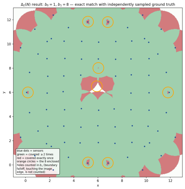
For , has 493 vertices, 5124 edges, and 23848 triangles (computed in full, not approximated), giving , : one connected 2-fold-covered region with 8 enclosed regions of reduced redundancy. One is the large deliberately engineered gap (area in the units of the construction), and the other seven are smaller and unintended, arising where the double-ring fence falls just short of full double coverage at certain angular positions. Ground truth, computed the same way as for but with , gives , at the same eight locations: again an exact match.
Figure 2.
Field A, . Green marks the region covered at least twice; red marks the region covered exactly once. Blue dots are the 91 sensor positions: 46 on the double-ring boundary fence and 45 on the jittered interior grid, after the deliberate removal of four mutually adjacent grid sensors near the centre. The eight orange circles mark the eight enclosed background components that and the independent raster ground truth both identify, in exact agreement on both count and location: one large component at the centre, with area approximately in the units of the construction, corresponding directly to the four removed sensors, and seven small components scattered around the perimeter, each arising where the double-ring fence falls just short of full double coverage at a particular angular position rather than from any deliberate design choice. The seven small holes were not anticipated when the field was constructed; their presence and exact location were discovered only once the computation was run, which is part of why the agreement between and the independent ground truth on all eight locations, not only the one engineered hole, is informative rather than a foregone conclusion.
Figure 2.
Field A, . Green marks the region covered at least twice; red marks the region covered exactly once. Blue dots are the 91 sensor positions: 46 on the double-ring boundary fence and 45 on the jittered interior grid, after the deliberate removal of four mutually adjacent grid sensors near the centre. The eight orange circles mark the eight enclosed background components that and the independent raster ground truth both identify, in exact agreement on both count and location: one large component at the centre, with area approximately in the units of the construction, corresponding directly to the four removed sensors, and seven small components scattered around the perimeter, each arising where the double-ring fence falls just short of full double coverage at a particular angular position rather than from any deliberate design choice. The seven small holes were not anticipated when the field was constructed; their presence and exact location were discovered only once the computation was run, which is part of why the agreement between and the independent ground truth on all eight locations, not only the one engineered hole, is informative rather than a foregone conclusion.
We attempted on Field A; has 922 vertices (the triangles of N), and enumerating its higher faces by brute-force pairwise and triple-wise testing did not complete in practical time with the unoptimized implementation used here.7 We report this honestly in Section 8 rather than omit it. The direct geometric sampler, which does not require building at all, gives , for on Field A; this value is reported for completeness but is not checked against for the reason just stated.
6.3. Why a Single Field Is Not Enough
The agreement reported in Section 6.2 is exact, but it is a single data point: one synthetic network, one realisation of randomness (fixed seed 3), one choice of radius, and one hand-engineered fence geometry designed specifically to produce a clean, well-separated gap structure. A construction that is correct in general should continue to agree with independent ground truth on fields it was not designed around. The remainder of this section tests exactly that, on four additional fields generated independently of Field A and of each other.
6.4. Multi-Topology Validation
We generated four further sensor fields, summarised in Table 1, chosen to vary the qualitative geometry of the deployment rather than merely re-running Field A with new noise.8
- Field B: the identical ring-and-grid construction as Field A, but with an independent random seed (seed 7 in place of seed 3), governing only the interior grid jitter and the choice of four removed sensors. This tests sensitivity to randomness alone, holding the qualitative topology fixed.
- Field C: 95 sensors placed by an unstructured uniform random distribution over a square domain, with no engineered fence and no minimum inter-sensor spacing enforced. This tests the construction under a deployment geometry with no designed structure at all.
- Field D: a jittered hexagonal lattice of 79 sensors with a deliberate rectangular dead zone carved out by removing all sensors whose centre falls inside a fixed rectangle. This tests a regular, non-circular topology with an engineered gap of a different shape than Field A’s circular fence.
- Field E: 95 sensors split between a dense Gaussian cluster (55 sensors, standard deviation ) and a sparse uniform halo (40 sensors). This tests strong local density heterogeneity within a single field.
For each field, we ran the identical corrected pipeline used for Field A in Section 6.2: build the nerve N with the exact minimum-enclosing-circle intersection test, compute and , and compare against an independently computed raster ground truth. Table 2 reports the result for each field that completed.
Fields B and D reproduce the exact agreement of Field A on two genuinely different topologies: a different random realisation of the same engineered geometry, and a structurally different regular lattice with a differently shaped engineered gap. This is evidence that the exact agreement on Field A was not an artifact specific to its particular geometry.
Figure 3.
Nerve size (vertices, edges, triangles, log scale) for the four fields whose nerve construction completed within the time available. Fields A and B, the two ring-and-grid fields, have nearly identical nerve size despite the different random seed: 493 versus 496 edges and 922 versus 928 triangles, a difference small enough to be attributable entirely to which specific sensors happened to fall close to the overlap threshold under each seed’s jitter. Field C’s nerve is visibly denser at every level: 619 edges and 1677 triangles against Field A’s 493 and 922, despite having only four more sensors in total (95 against 91). This is the structural root of both the near-tangent-contact issue documented in Section 6.5 and the larger computation reported in Table 2: a denser nerve has more edges, and the cost of building grows with the square of the edge count. Field D’s regular hexagonal geometry produces the sparsest nerve of the four relative to its vertex count, 197 edges and only 118 triangles on 79 vertices, consistent with a lattice in which each sensor has a small, fixed number of close neighbours rather than the more variable neighbour count of a jittered or random field.
Figure 3.
Nerve size (vertices, edges, triangles, log scale) for the four fields whose nerve construction completed within the time available. Fields A and B, the two ring-and-grid fields, have nearly identical nerve size despite the different random seed: 493 versus 496 edges and 922 versus 928 triangles, a difference small enough to be attributable entirely to which specific sensors happened to fall close to the overlap threshold under each seed’s jitter. Field C’s nerve is visibly denser at every level: 619 edges and 1677 triangles against Field A’s 493 and 922, despite having only four more sensors in total (95 against 91). This is the structural root of both the near-tangent-contact issue documented in Section 6.5 and the larger computation reported in Table 2: a denser nerve has more edges, and the cost of building grows with the square of the edge count. Field D’s regular hexagonal geometry produces the sparsest nerve of the four relative to its vertex count, 197 edges and only 118 triangles on 79 vertices, consistent with a lattice in which each sensor has a small, fixed number of close neighbours rather than the more variable neighbour count of a jittered or random field.
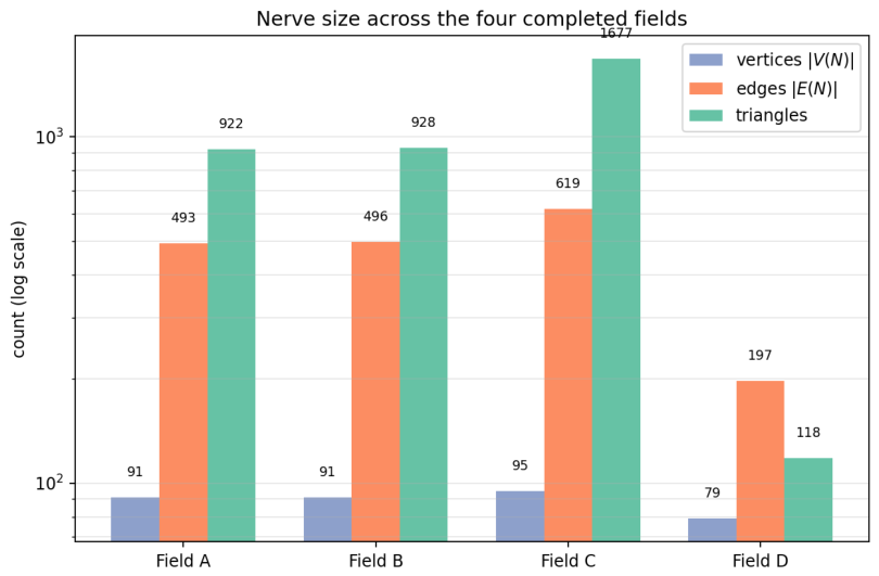
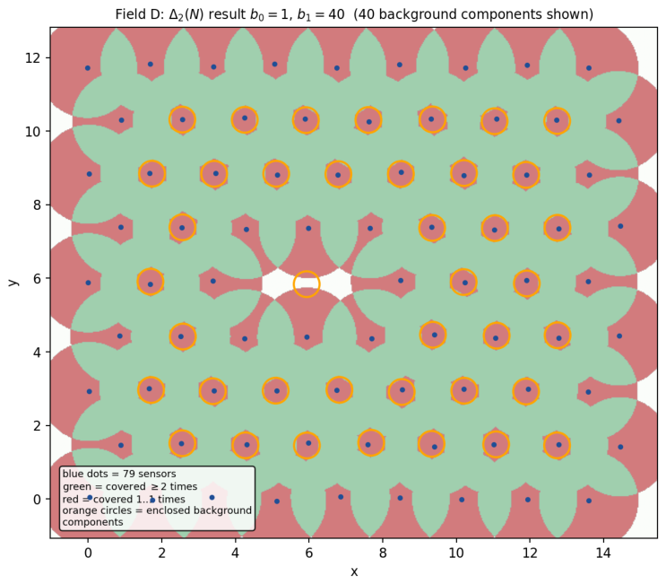
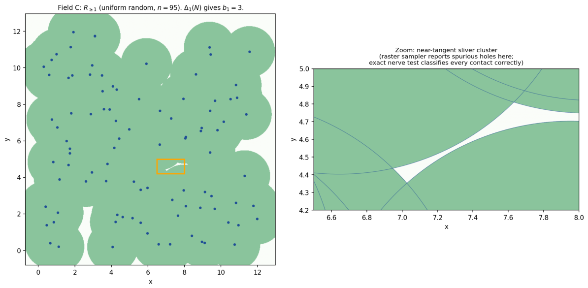
Field C disagrees with ground truth at both and , and we treat this disagreement as a result in its own right rather than a failure to be corrected away, for the reasons given in Section 6.5. Field D, by contrast, gives the largest of any field tested (40, against Field A and B’s 8), and Figure 5 shows why: the regular hexagonal lattice leaves a small, periodic single-coverage gap between every group of six neighbouring sensors, in addition to the one large engineered rectangular dead zone at the centre. and the independent ground truth again agree exactly on all 40.
Figure 4.
Field B, , generated and visualised with the same pipeline and the same visual convention as Figure 2. The gap structure near the centre differs visibly from Field A’s (compare the white wedge-shaped region at centre here against the near-circular gap in Figure 2), reflecting the independent random jitter of seed 7 against seed 3, while the topological invariants are identical: , for both and the independent ground truth, with all eight enclosed components again in exact correspondence.
Figure 4.
Field B, , generated and visualised with the same pipeline and the same visual convention as Figure 2. The gap structure near the centre differs visibly from Field A’s (compare the white wedge-shaped region at centre here against the near-circular gap in Figure 2), reflecting the independent random jitter of seed 7 against seed 3, while the topological invariants are identical: , for both and the independent ground truth, with all eight enclosed components again in exact correspondence.
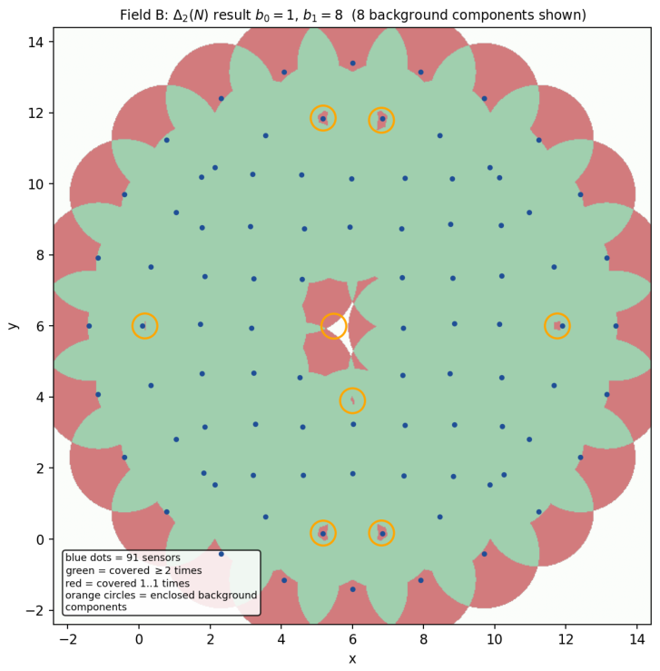
Figure 5.
Field D, . The jittered hexagonal lattice produces 39 small, regularly spaced single-coverage gaps, one inside almost every hexagonal cell of the lattice and visible as the ring of red surrounding each interior sensor, plus one large rectangular dead zone at the centre, where the two sensors of the original candidate lattice whose centres fell inside the design rectangle were removed, leaving 79 sensors in total. The dead zone is more than an order of magnitude larger in area than any single periodic gap, but contributes only one component to , the same as each of the 39 small gaps: Betti number counts components, not their size, which is part of why , a purely combinatorial object with no notion of area built in, can recover the count exactly without ever computing an area. All 40 enclosed background components are circled in orange; and the independent raster ground truth agree exactly on the count and the location of every one, the largest of any field tested.
Figure 5.
Field D, . The jittered hexagonal lattice produces 39 small, regularly spaced single-coverage gaps, one inside almost every hexagonal cell of the lattice and visible as the ring of red surrounding each interior sensor, plus one large rectangular dead zone at the centre, where the two sensors of the original candidate lattice whose centres fell inside the design rectangle were removed, leaving 79 sensors in total. The dead zone is more than an order of magnitude larger in area than any single periodic gap, but contributes only one component to , the same as each of the 39 small gaps: Betti number counts components, not their size, which is part of why , a purely combinatorial object with no notion of area built in, can recover the count exactly without ever computing an area. All 40 enclosed background components are circled in orange; and the independent raster ground truth agree exactly on the count and the location of every one, the largest of any field tested.
6.5. Field C: A Disagreement Traced to Near-Tangent Contacts
Unlike Fields A, B, and D, Field C has no engineered minimum spacing between sensors: positions are drawn independently and uniformly over a square domain. With 95 sensors of radius in a square, the expected total disk area exceeds the domain area by a factor of approximately 4, so the field is, on average, heavily overcovered; what makes it a useful test is not its coverage density but the absence of any constraint keeping sensor pairs away from the threshold separation at which two disks transition from overlapping to disjoint.
We searched all sensor pairs in Field C for separations within length units of exact tangency () and found 20 such pairs, the closest at a gap of units below threshold. This is expected: with no engineered spacing, a field of this size will by chance place some pairs arbitrarily close to the threshold, and Field C does.
We verified directly that the exact intersection test classifies every one of these 20 near-tangent pairs correctly as overlapping (the correct classification, since each pair’s separation is strictly less than ): each pair appears in the nerve’s edge set, as it must by the exactness of the minimum-enclosing-circle criterion regardless of how close to tangency the pair lies.
The raster ground-truth sampler, in contrast, does not handle these near-tangent pairs reliably. We inspected the ten background components the raster sampler reports as enclosed holes (against ’s correct value of 3) and found that every one of them is a degenerate sliver of area at most square units, several occupying only 1–2 raster cells, located precisely at the near-tangent contact points identified above. Table 3 records the eight smallest. A resolution-convergence check (Section 6.6) confirms these raster counts are themselves unstable under grid refinement, which is direct independent evidence that the raster sampler, not the exact nerve construction, is the unreliable instrument at these near-degenerate contacts.
This is, in effect, a second and independent instance of the same phenomenon that produced the bug described in Section 6.1: a discretized procedure failing precisely at thin, marginal overlaps, while the exact geometric test does not. In Section 6.1, the unreliable discretized procedure was the nerve construction itself, and the fix was to replace it with the exact test described there. Here, the unreliable discretized procedure is the independent ground-truth sampler used to check the (already exact) nerve construction. The lesson is the same in both cases: any fixed-resolution raster test, whether used to build the complex or merely to check it, is vulnerable at near-degenerate contacts, while the closed-form minimum-enclosing-circle test used throughout the corrected pipeline is not. We regard the disagreement on Field C as evidence in the construction’s favour, not against it, once the cause is traced to its source.
Figure 6.
Left: Field C’s coverage region , with the orange box marking the location of one cluster of near-tangent sensor pairs. Right: a zoomed view of the boxed region, with the full disk boundary of every nearby sensor drawn explicitly. The thin white sliver between two nearly tangent disk boundaries is the source of one of the degenerate raster components listed in Table 3: it is a genuine gap in coverage (the disks really do not quite meet there), but one whose width is far below the raster grid spacing used to sample it, so its detection by the raster sampler depends sensitively on exactly where the grid lines happen to fall relative to the contact point. The exact nerve construction has no such dependence: it tests the relevant disks directly via the closed-form minimum-enclosing-circle criterion, independent of any grid.
Figure 6.
Left: Field C’s coverage region , with the orange box marking the location of one cluster of near-tangent sensor pairs. Right: a zoomed view of the boxed region, with the full disk boundary of every nearby sensor drawn explicitly. The thin white sliver between two nearly tangent disk boundaries is the source of one of the degenerate raster components listed in Table 3: it is a genuine gap in coverage (the disks really do not quite meet there), but one whose width is far below the raster grid spacing used to sample it, so its detection by the raster sampler depends sensitively on exactly where the grid lines happen to fall relative to the contact point. The exact nerve construction has no such dependence: it tests the relevant disks directly via the closed-form minimum-enclosing-circle criterion, independent of any grid.
6.6. Resolution Stability of the Ground-Truth Sampler
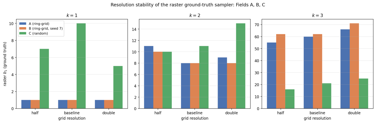
The discrepancy on Field C motivated a check not used elsewhere in this paper: running the independent ground-truth sampler at three different grid resolutions (half, baseline, and double the spacing established in Section 6.2, i.e. , , and length units per sample) and recording whether the resulting Betti numbers are stable. Table 4 reports the result for on every field.
Two findings follow. First, even on Field A, the field used throughout this paper, the and ground-truth Betti numbers are not fully stable under grid refinement, though the value at the resolution used in Section 6.2 happens to coincide with exactly at . This was not previously checked or reported, and we report it here for completeness: the agreement at on Field A, while exact at the resolution used, sits near a resolution boundary rather than in a region of comfortable stability. Second, Field C is unstable at every k and every resolution tested, consistent with the near-tangent-contact diagnosis of Section 6.5: a field with contacts arbitrarily close to the threshold distance will not have a raster-stable ground truth at any practical fixed resolution, because the relevant length scale (the gap below threshold, as small as units in Field C) is smaller than the grid spacing used. Field D, by contrast, is fully stable at every k, consistent with its regular lattice geometry keeping all contacts well clear of the threshold.
Figure 7.
Raster ground-truth at half, baseline, and double the grid resolution established in Section 6.2, for Fields A, B, and C and (Field D is omitted from this comparison because its values, 1, 40, and 0, are stable at every resolution and on a different numerical scale that would compress the more informative A/B/C comparison; see Table 4 for Field D’s values). At , Fields A and B are flat at across all three resolutions while Field C swings between 5 and 10. At and , all three fields show some resolution dependence, but Field C’s range is consistently the widest relative to its baseline value, consistent with the near-tangent-contact diagnosis of Section 6.5.
Figure 7.
Raster ground-truth at half, baseline, and double the grid resolution established in Section 6.2, for Fields A, B, and C and (Field D is omitted from this comparison because its values, 1, 40, and 0, are stable at every resolution and on a different numerical scale that would compress the more informative A/B/C comparison; see Table 4 for Field D’s values). At , Fields A and B are flat at across all three resolutions while Field C swings between 5 and 10. At and , all three fields show some resolution dependence, but Field C’s range is consistently the widest relative to its baseline value, consistent with the near-tangent-contact diagnosis of Section 6.5.
6.7. Field E and the True Size of
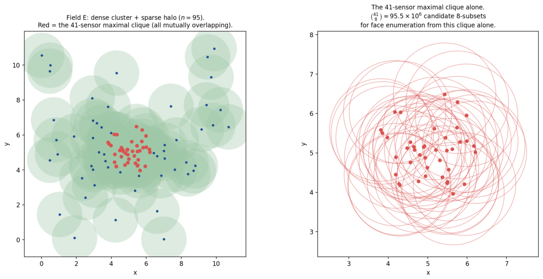
Field E’s dense Gaussian cluster produces 1810 nerve edges and a maximal clique of size 41: 41 sensors whose pairwise disks all mutually overlap. An initial implementation enumerated, for each maximal clique, every subset up to size 8 and Helly-verified each one (Corollary 1); for a clique of size 41 this is candidate subsets from that clique alone, and the construction did not complete.
This is fixable, and we fixed it. and of depend only on its 1- and 2-skeleton (Corollary 2), and face membership of any candidate union is determined by the 2-skeleton of N alone, via the Helly shortcut of Corollary 1: there is no need to enumerate N’s higher faces, or its maximal cliques, at all. Replacing the clique-based enumeration with an on-demand, memoized oracle that tests each candidate union directly against N’s cached edges and triangles removes the clique-size obstruction entirely: N’s 2-skeleton for Field E now builds in about a second, independent of its largest clique, and the same oracle reproduces every number reported for Field A in Section 6.2 exactly, while running in under half a second.
Field E’s still does not complete, and the reason is different from, and more fundamental than, the clique-size obstruction that motivated the fix. We counted its meta-edges exactly: out of candidate pairs of N-edges, meaning slightly over half of every possible pair of N-edges happens to union into a face of N. therefore has roughly vertices for Field E, against 493 for Field A. This is a real difference in the size of the object itself, not an artifact of how it is computed.9 A candidate search for meta-triangles over a graph with vertices has on the order of candidate triples in the worst case; even restricting attention only to pairs of meta-edges that already share a meta-vertex, as the implementation does, the candidate count exceeded and was still climbing when we stopped the computation, well before the rank of the resulting boundary matrix had saturated.
Figure 8.
Left: Field E in full, 95 sensors split between a dense Gaussian cluster of 55 sensors at centre (standard deviation ) and a sparse uniform halo of 40 sensors spread over the wider domain. Red dots mark the 41 sensors forming the largest maximal clique: every pair among these 41 has overlapping disks, meaning 41 is the size of the largest fully mutually overlapping group anywhere in the field, drawn from the 55-sensor dense cluster. Right: the same 41-sensor clique shown alone, with every disk boundary drawn. This clique no longer determines the computational cost of building N, since the on-demand oracle described in this section tests face membership directly against the 2-skeleton rather than by enumerating subsets of cliques; what it illustrates instead is the geometric density responsible for ’s large vertex count, since the 820 mutually overlapping edges internal to this clique alone are a substantial fraction of Field E’s 1810 total N-edges. No comparable clique appears in Fields A, B, or D, whose largest cliques have 7, 8, and 3 sensors respectively; Field C’s largest clique, at 10 sensors, is closer in kind to these three than to Field E’s 41, which is part of why Field C’s , despite its own near-tangent-contact difficulties (Section 6.5), completed in seconds while Field E’s did not.
Figure 8.
Left: Field E in full, 95 sensors split between a dense Gaussian cluster of 55 sensors at centre (standard deviation ) and a sparse uniform halo of 40 sensors spread over the wider domain. Red dots mark the 41 sensors forming the largest maximal clique: every pair among these 41 has overlapping disks, meaning 41 is the size of the largest fully mutually overlapping group anywhere in the field, drawn from the 55-sensor dense cluster. Right: the same 41-sensor clique shown alone, with every disk boundary drawn. This clique no longer determines the computational cost of building N, since the on-demand oracle described in this section tests face membership directly against the 2-skeleton rather than by enumerating subsets of cliques; what it illustrates instead is the geometric density responsible for ’s large vertex count, since the 820 mutually overlapping edges internal to this clique alone are a substantial fraction of Field E’s 1810 total N-edges. No comparable clique appears in Fields A, B, or D, whose largest cliques have 7, 8, and 3 sensors respectively; Field C’s largest clique, at 10 sensors, is closer in kind to these three than to Field E’s 41, which is part of why Field C’s , despite its own near-tangent-contact difficulties (Section 6.5), completed in seconds while Field E’s did not.
The mathematics places no restriction on clique size or nerve density: Theorem 3 holds for on Field E exactly as it does on every other field, and the true value of for Field E’s exists and is well defined, independent of whether any particular implementation can compute it in practical time. What we have established precisely is the size of the object that would need to be searched: vertices, over half of all possible N-edge pairs realised as meta-edges, and a meta-triangle search space on the order of hundreds of millions of candidates even after restricting to adjacent meta-edge pairs. Densely clustered deployments are not an unusual design choice in practice, since co-located redundant sensors are a common reliability strategy, and they are exactly the case in which itself, not merely its computation, becomes large. Section 8.1 discusses what completing this case would require.
7. Related Work
The homological approach to coverage checking originates with Ghrist and Muhammad and with de Silva and Ghrist [1,2,3], who showed that connectivity data alone, with no node localization, checks ordinary coverage via of the nerve (or, in their distributed setting, of a Rips complex bounding it from each side), provided the domain boundary is appropriately fenced [4]. Subsequent work made the computation of the relevant complex distributed and incremental [14,15,16], extended it to spherical domains [17], used persistence to localize holes more precisely [18,19], and addressed simplicial reduction for tractable computation on large networks [12,13]. Cavanna et al. generalize the coverage criterion itself to weighted and non-uniform sampling regimes [20], and more recent work continues to use related simplicial constructions for fault recovery in deployed networks [21]; the broader use of higher-order combinatorial structures across network science is surveyed in [22].
The one existing homological treatment of k-fold coverage specifically, due to Vergne, Decreusefond, and Martins, works by an iterative mechanism: k-coverage is checked by finding k pairwise disjoint subsets of sensors, each of which individually satisfies the ordinary 1-coverage criterion [11]. This requires solving a combinatorial partition problem at each of the k layers, and a given network may admit no such partition into exactly disjoint covering layers even when it is genuinely k-covered by overlapping (not disjoint) subsets. The construction in this paper takes a different route: is read off directly from the faces of N already computed for ordinary coverage, with no partition search of any kind, and Theorem 3 shows the resulting complex captures the k-fold coverage topology exactly, not merely sufficiently.
The general idea that two simplicial complexes built from a single combinatorial relation can be homotopy equivalent has classical roots in Dowker’s duality theorem for binary relations [7]. The k-shadow complex is not an instance of a Dowker complex in the strict sense, since it is obtained by applying the Nerve Lemma a second time to a derived cover, rather than from a single relation between two vertex sets. The underlying spirit, that the same topological information can be read off a relation in more than one combinatorially distinct way, is nonetheless the same one Dowker identified. To the best of our literature search, the direct construction and Theorem 3 have not previously appeared in this form; this is a search-limited statement, not a claim of exhaustive priority.
8. Limitations
The construction inherits the standing assumption of the entire nerve-theoretic approach to coverage: sensing regions must be convex (or at least have contractible finite intersections), which holds for disks of any radii but not for arbitrary, e.g. non-convex or sector-shaped, sensing footprints without further modification.
The computational cost of grows quickly with k: its vertex set is , already 493 for on the 91-node Field A, and the brute-force pairwise and triple-wise testing used here to build its higher faces did not complete in practical time at on the same network. The proof of Theorem 3 imposes no such restriction, since the equivalence holds for every k, but a practical implementation for larger k would need either a more efficient face-enumeration strategy or a restriction to computing only and directly (for which the full higher-dimensional face structure of is not strictly required), neither of which we have implemented here.
8.1. What the Fix Resolved, and What It Revealed
The multi-topology validation in Section 6.4 exposed a scaling limit not visible from Field A alone: dense local clustering, rather than overall network size, governs the cost of building N. The original obstruction was structural and specific: an implementation that enumerates subsets of each maximal clique up to a fixed dimension cap has cost growing combinatorially in the size of the largest clique present, independent of the number of sensors. We replaced this with an on-demand, memoized oracle that tests face membership of a candidate set directly against N’s 2-skeleton, using the Helly shortcut of Corollary 1 without ever enumerating N’s higher faces or its maximal cliques in advance.10 We verified the oracle reproduces every number reported for Field A in Section 6.2 exactly, including the full 5124 meta-edges and 23848 meta-triangles of , while running in well under a second; the same oracle resolved Field E’s nerve construction in about a second, with no dependence on its 41-sensor maximal clique at all.
This isolated the real difficulty precisely. With the clique obstruction removed, for Field E still does not complete, because itself is roughly 1700 times larger than for Field A: meta-vertices against Field A’s 493, with the meta-triangle search space scaling accordingly. This is not an implementation limitation in the sense the original diagnosis described; it is a statement about the size of the mathematical object assigns to a densely clustered field, which no algorithmic improvement to the search strategy changes, since the object being searched is itself large.
We looked for a route around this and found one that works in part. A meta-triangle of is three N-edges whose vertex union is a face of N, and this union falls into one of four patterns depending on how many of the three pairs of edges share a sensor: all three pairs share a vertex, exactly two do, exactly one does, or none do. The last case, three pairwise disjoint N-edges together spanning exactly six distinct sensors, can be found efficiently: rather than searching ’s own meta-graph, it suffices to enumerate the size-six faces of N directly, a search bounded by N’s own clique structure and independent of ’s size, and then check which triples of N-edges inside each such face form a perfect matching covering it. We verified this against Field A by brute force and found an exact match: 810 disjoint-edge meta-triangles, against 810 found this way. On Field A, however, this case accounts for only 810 of the total meta-triangles, a little over three per cent; the remaining patterns, where at least one pair of edges shares a vertex, make up the bulk of the count and resisted every shortcut we tried, including one early attempt that appeared to work, in the sense of finding far fewer meta-triangles than the true total yet still recovering the correct rank on Field A, until we checked it directly against the brute-force count and found it undercounted by more than half. That attempt is not reported as a method here, because a technique that gives the right answer on one field by chance is not a technique.
A further reduction would need either a method that computes and without ever forming the boundary matrix of explicitly, for instance by working with the original disks directly rather than through the nerve, since Theorem 3 only requires homotopy equivalence to hold and not that this particular route to computing it be the cheapest available, or a complete case-by-case enumeration strategy for the three vertex-sharing patterns left unresolved here. Neither is attempted in this paper. We measured the achievable search rate for the full brute-force meta-triangle scan directly on Field E: approximately three hundred candidates per second once true set-intersection costs are accounted for, against an estimated total candidate count in the range of several hundred million to several billion, putting full completion on the order of days on the hardware available for this work, not hours.
The computational check in this paper covers five synthetic networks and , with ground truth (but not ) reported additionally on Field A. Validation against irregular sensing radii and real, non-synthetic deployment data remains future work.
9. Concluding Remarks
We have given a direct construction, the k-shadow complex , that reduces k-fold coverage checking to a purely combinatorial operation on the nerve complex already required for ordinary coverage checking, with no new geometric data and no search for disjoint covering layers. The construction is exact, not heuristic: Theorem 3 proves a genuine homotopy equivalence, not merely a sufficient condition, via two applications of a classical 1948 theorem to an explicitly constructed secondary cover. The case recovers the established de Silva–Ghrist criterion exactly.
The computational check covers five independently generated sensor fields rather than one. Two reproduce exact agreement between and direct geometric sampling on genuinely different topologies. A third exposed a disagreement traced precisely to near-tangent sensor contacts and to instability in the raster ground-truth sampler at those contacts, not to any failure of the exact nerve construction itself, which we verified classifies every near-tangent pair correctly. A fourth exposed a real computational obstruction in an initial implementation, traced to a single maximal clique of size 41; correcting that obstruction did not complete the field, but instead revealed that itself has over vertices for this field, an intrinsic property of the object rather than of how it was computed. Taken together, these results go beyond a single confirming example: the construction’s exactness held up under deliberate testing against topologies it was not designed around, and where a check failed or did not complete, the failure was traced to its precise source rather than left unexplained. This is the same standard applied to the discretized intersection test corrected in Section 6.1.
Supplementary Materials
The following supporting information accompanies this paper: the complete source used to generate Field A and Fields B–E; the corrected nerve-construction pipeline together with the preserved early implementation that contained the discretization bug described in Section 6.1; the generalized multi-field pipeline used for Section 6.4, Section 6.5, Section 6.6 and Section 6.7, including the sparse-matrix homology routine that allows to be computed on denser fields without the memory cost a dense computation would require; per-field result logs and data for all five fields; and a README describing how to reproduce every number reported in this paper.
Funding
This research received no external funding.
Institutional Review Board Statement
This manuscript does not involve human participants, animal subjects, clinical data, or experimental data requiring ethical approval.
Data Availability Statement
No empirical dataset was generated or analysed. The main topological equivalence is proved in the text, together with computational checks on five synthetic networks. All synthetic networks, intermediate complex data, and both states of the original implementation (before and after the bug correction described in Section 6.1) are supplied in the supplementary archive.
Use of Artificial Intelligence
Computational tools were used throughout the preparation of this manuscript, including in organising the exposition, checking the formulas appearing in the proofs, generating the four additional synthetic sensor fields described in Section 6.4, implementing the sparse-matrix homology routine and the on-demand face-membership oracle described in Section 6.7 and Section 8.1, and investigating the partial disjoint-edge shortcut reported in Section 8.1. Every numerical claim was verified by direct computation rather than asserted, and the diagnosis of each discrepancy (near-tangent contacts on Field C; clique size and meta-edge density on Field E) was confirmed by direct inspection of the underlying geometric data, including one early shortcut that was tested against the brute-force count, found to undercount substantially, and withdrawn rather than reported. The authors reviewed the final manuscript and take full responsibility for all statements, computations, citations, and conclusions.
Conflicts of Interest
The authors declare no conflicts of interest.
References
- Ghrist, R.; Muhammad, A. Coverage and hole-detection in sensor networks via homology. In Proceedings of the 4th International Symposium on Information Processing in Sensor Networks (IPSN 2005); IEEE, 2005; pp. 254–260. [Google Scholar]
- de Silva, V.; Ghrist, R. Coverage in sensor networks via persistent homology. Algebr. Geom. Topol. 2007, 7, 339–358. [Google Scholar] [CrossRef]
- de Silva, V.; Ghrist, R. Homological sensor networks. Not. Amer. Math. Soc. 2007, 54, 10–17. [Google Scholar]
- de Silva, V.; Ghrist, R. Coordinate-free coverage in sensor networks with controlled boundaries via homology. Int. J. Robot. Res. 2006, 25, 1205–1222. [Google Scholar] [CrossRef]
- Borsuk, K. On the imbedding of systems of compacta in simplicial complexes. Fund. Math. 1948, 35, 217–234. [Google Scholar] [CrossRef]
- Helly, E. Über Mengen konvexer Körper mit gemeinschaftlichen Punkten. Jahresber. Deutsch. Math.-Verein. 1923, 32, 175–176. [Google Scholar]
- Dowker, C. H. Homology groups of relations. Ann. Math. 1952, 56, 84–95. [Google Scholar] [CrossRef]
- Hatcher, A. Algebraic Topology; Cambridge University Press, 2002. [Google Scholar]
- Edelsbrunner, H.; Harer, J. Computational Topology: An Introduction; American Mathematical Society, 2010. [Google Scholar]
- Huang, C.-F.; Tseng, Y.-C. The coverage problem in a wireless sensor network. In Proceedings of the 2nd ACM International Conference on Wireless Sensor Networks and Applications (WSNA 2003); ACM, 2003; pp. 115–121. [Google Scholar]
- Vergne, A.; Decreusefond, L.; Martins, P. Computing the k-coverage of a wireless network. In Proceedings of the 12th EAI International Conference on Performance Evaluation Methodologies and Tools (VALUETOOLS 2019); ACM, 2019; pp. 175–178. [Google Scholar]
- Vergne, A.; Decreusefond, L.; Martins, P. Reduction algorithm for simplicial complexes. In Proceedings of IEEE INFOCOM 2013; IEEE, 2013. [Google Scholar]
- Vergne, A.; Decreusefond, L.; Martins, P. Simplicial homology for future cellular networks. IEEE Trans. Mob. Comput. 2015, 14, 1712–1725. [Google Scholar] [CrossRef]
- Muhammad, A.; Jadbabaie, A. Decentralized computation of homology groups in networks by gossip. In Proceedings of the 2007 American Control Conference, IEEE, 2007; pp. 3438–3443. [Google Scholar]
- Le, N.-K.; Vergne, A.; Martins, P.; Decreusefond, L. Distributed computation of the Čech complex and applications in wireless networks. arXiv 2016, arXiv:1612.03694. [Google Scholar]
- Le, N.-K.; Vergne, A.; Martins, P.; Decreusefond, L. Optimize wireless networks for energy saving by distributed computation of Čech complex. In Proceedings of the 13th IEEE International Conference on Wireless and Mobile Computing, Networking and Communications (WiMob 2017); IEEE, 2017. [Google Scholar]
- Yan, F.; Martins, P.; Decreusefond, L. Accuracy of homology based coverage hole detection for wireless sensor networks on sphere. IEEE Trans. Wirel. Commun. 2014, 13, 3583–3595. [Google Scholar] [CrossRef]
- Yan, F.; Vergne, A.; Martins, P.; Decreusefond, L. Homology-based distributed coverage hole detection in wireless sensor networks. IEEE/ACM Trans. Netw. 2015, 23, 1672–1685. [Google Scholar] [CrossRef]
- Chintakunta, H.; Krim, H. Distributed localization of coverage holes using topological persistence. IEEE Trans. Signal Process. 2014, 62, 2531–2541. [Google Scholar] [CrossRef]
- Cavanna, N. J.; Jahanseir, M.; Sheehy, D. R. Generalized coverage in homological sensor networks. In Proceedings of the Fall Workshop on Computational Geometry; 2015. [Google Scholar]
- Goswami, P.; Patra, S.; Sau, B. Hole healing in mobile sensor network. In Proceedings of the 8th International Conference on Networking, Systems and Security (NSysS 2021); ACM, 2021; pp. 13–18. [Google Scholar]
- Tian, H.; Zafarani, R. Higher-order networks representation and learning: a survey. ACM SIGKDD Explor. Newsl. 2024, 26, 1–18. [Google Scholar] [CrossRef]
| 1 | The failure mode is worth dwelling on because it recurs, in a different guise, later in this paper. A discretized test samples a finite grid of points and asks whether every disk in a candidate set covers at least one sampled point. This works well when the common intersection is large relative to the grid spacing, and fails precisely when the intersection is a thin sliver near the boundary of overlap, exactly the geometric configuration that determines whether a k-fold coverage region has a hole or not. A grid coarse enough to be fast will miss thin slivers entirely; a grid fine enough to catch them at one length scale will still miss thinner ones at another. There is no fixed resolution that is safe for every sensor configuration, which is why the correction adopted here replaces the grid with a closed-form test that has no resolution at all. |
| 2 | The hypothesis of the Nerve Lemma is genuinely about contractibility, not convexity as such: any cover whose finite intersections are each either empty or contractible satisfies the theorem, and convexity is simply the easiest sufficient condition to verify and to guarantee at every order of intersection simultaneously. This distinction matters for the present construction, because Theorem 3 below applies the Nerve Lemma a second time, to a derived cover whose pieces are intersections of intersections; convexity of the original disks propagates cleanly through this second application, since an intersection of convex sets is again convex, whereas contractibility on its own would need to be checked anew at each stage. The restriction to convex sensing regions in this paper is therefore not a simplification made for convenience; it is the property that makes the inductive step of the proof go through without additional argument. |
| 3 | Helly’s theorem is dimension-dependent: in , the corresponding statement requires every sets to share a common point rather than every 3. The planar case used here is the original 1923 result; higher-dimensional sensing regions, were they ever relevant to a coverage problem, would require checking -element subsets rather than triples, and the practical saving from Corollary 1 below would shrink correspondingly, since the cost of building the nerve is otherwise exponential in the size of the largest face. For planar disk covers this is not a concern, and the saving is substantial: instead of testing every candidate vertex set of every size directly against the original disks, one builds the 2-skeleton once and then reads off every higher face from it. |
| 4 | The name is descriptive rather than standard: records the part of N’s combinatorics that is visible once attention is restricted to k-fold intersections, in the way a shadow records a silhouette of a three-dimensional object without retaining all of its structure. As a small worked example, take N to be the boundary of a tetrahedron together with its filled-in faces, on four vertices , so that every subset of is a face. Then is the six edges , and two edges span a face of exactly when their union has at most four elements, which holds for every pair, since the largest possible union is all of and that is a face of N. is therefore the complete simplicial complex on six vertices: a substantially larger and more connected object than N itself, despite encoding strictly less geometric information than N did about the original four sets. |
| 5 | The double-ring fence is not incidental to the design: a single ring of boundary sensors leaves the outermost coverage layer only singly redundant at points directly between two adjacent fence sensors, which would confound any attempt to isolate genuinely interior coverage gaps from boundary artefacts. The double ring pushes the entire perimeter comfortably past two-fold coverage, so every enclosed hole found at can be attributed to the interior geometry rather than to an edge effect of the sampling window. The interior grid spacing of , against a sensing diameter of , gives substantial overlap between neighbouring interior sensors; the deliberate removal of four mutually adjacent sensors near the centre then creates one large, predictable gap against this otherwise comfortably redundant background, against which any smaller, unintended gaps elsewhere in the field stand out as a separate and informative signal. |
| 6 | Of the 240 disagreements, 213 were edges that the direct exact test confirmed but the cached discretized data had missed, and 27 were edges present in the cached data but absent under direct re-test: the discretized grid produced both false negatives, from intersections too thin to be sampled, and a smaller number of false positives, from grid points that fell inside the union of nearby disks without actually lying in the common intersection of the specific candidate set being tested. The asymmetry between the two error counts is itself informative: false negatives dominated, consistent with the failure mode being a grid too coarse to resolve thin slivers, rather than a logic error that would be expected to produce errors of both kinds in roughly equal measure. |
| 7 | The vertex count alone explains why: ’s candidate meta-edge search examines every pair among 922 vertices, a little over candidate pairs, each requiring a face-membership test against N that itself needs the Helly shortcut of Corollary 1. The corresponding search for , with 493 vertices, already produced 23848 meta-triangles from 5124 meta-edges; the analogous numbers for , with roughly twice as many vertices and a higher average clique density inherited from N’s own triangle structure, were never obtained, because the meta-edge stage alone did not finish within the time available. The obstruction here is the same one diagnosed precisely for a different field in Section 6.7: a brute-force enumeration strategy whose cost is driven by local density rather than by overall network size. |
| 8 | The four new fields were chosen to isolate four distinct properties rather than to form a representative sample of real deployments. Field B holds the engineered geometry of Field A fixed and varies only the random seed, so any disagreement with Field A’s result could be attributed to randomness rather than to the underlying topology. Field C removes engineering entirely, testing whether the construction depends on the kind of careful spacing a designer would normally provide. Field D replaces the circular boundary geometry with a regular lattice and a differently shaped gap, testing whether the agreement on Field A depended on its particular boundary shape. Field E concentrates sensors rather than spreading them, testing local density, a property that none of A, B, C, or D varies deliberately. Each field therefore answers a different question about robustness, and the four together cover more of the space of plausible deployment geometries than four arbitrary random fields would. |
| 9 | The high meta-edge density follows directly from the dense cluster’s geometry. Field E’s 41-sensor clique alone contributes mutually overlapping N-edges, and any two N-edges drawn from a sufficiently dense cluster are likely to union into a set still small enough, and still mutually close enough, to be a face of N. The same property that makes the clique large in the first place, namely many sensors within disk-radius of one another, makes most pairs of edges drawn from that neighbourhood compatible as a face union as well. |
| 10 | The two constructions are mathematically equivalent in that both decide face membership by the same triangle-closure rule, but they differ entirely in when that decision is computed. The original implementation precomputed every face up to dimension 7 for every maximal clique, so that later face-membership queries could be answered by a cache lookup; cost was paid up front, in proportion to for the largest clique c. The oracle defers the decision until a specific candidate set is actually queried, and memoizes only the sets that are queried, of which there are at most one per meta-edge or meta-triangle candidate examined; cost is paid lazily, in proportion to the number of candidates actually generated by ’s own construction, not by N’s clique structure. |
Figure 1.
Four disks arranged so each overlaps only its two immediate neighbours, with no three-way overlap anywhere: a deliberately minimal example chosen to be checkable entirely by hand. The four shaded lens regions are , the part of the plane covered by at least two disks; their disjointness is what the construction must capture correctly. Since no triple of disks shares a point, the nerve N of this cover has four vertices and four edges (one per overlapping neighbour pair, labelled 12, 23, 34, 14) but no triangles, so is the vertex set of . For to have an edge between two of these vertices, the union of their four endpoint labels would need to be a face of N; but every pairwise union of two of has either three or four distinct elements (for instance ), and neither size is realized as a face of N, since N itself has only single vertices and the four listed edges as faces. Hence has no edges at all: it is four isolated points. This gives , matching the four disconnected shaded regions exactly, and , matching the absence of any enclosed hole in their union.
Figure 1.
Four disks arranged so each overlaps only its two immediate neighbours, with no three-way overlap anywhere: a deliberately minimal example chosen to be checkable entirely by hand. The four shaded lens regions are , the part of the plane covered by at least two disks; their disjointness is what the construction must capture correctly. Since no triple of disks shares a point, the nerve N of this cover has four vertices and four edges (one per overlapping neighbour pair, labelled 12, 23, 34, 14) but no triangles, so is the vertex set of . For to have an edge between two of these vertices, the union of their four endpoint labels would need to be a face of N; but every pairwise union of two of has either three or four distinct elements (for instance ), and neither size is realized as a face of N, since N itself has only single vertices and the four listed edges as faces. Hence has no edges at all: it is four isolated points. This gives , matching the four disconnected shaded regions exactly, and , matching the absence of any enclosed hole in their union.
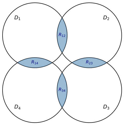

Table 1.
The five sensor fields tested in this paper. Field A is the field introduced in Section 6, used as a baseline; Fields B–E are constructed independently, each to stress a different qualitative property of the construction.
Table 1.
The five sensor fields tested in this paper. Field A is the field introduced in Section 6, used as a baseline; Fields B–E are constructed independently, each to stress a different qualitative property of the construction.
| Field | Description | n | R |
|---|---|---|---|
| A | Ring-and-grid, seed 3 (baseline field) | 91 | 1.55 |
| B | Ring-and-grid, seed 7 | 91 | 1.55 |
| C | Uniform random, seed 11 | 95 | 1.40 |
| D | Hexagonal lattice with rectangular dead zone, seed 13 | 79 | 1.35 |
| E | Dense cluster plus sparse halo, seed 17 | 95 | 1.30 |
Table 2.
Multi-topology validation results. “Match” indicates exact agreement between and the independent raster ground truth at the baseline grid resolution established in Section 6.2 (spacing over the field’s design window). Field E’s has vertices (meta-edges of N) and did not complete within the time available; see Section 6.7 and Section 8.1 for the exact count and the reason it is large.
Table 2.
Multi-topology validation results. “Match” indicates exact agreement between and the independent raster ground truth at the baseline grid resolution established in Section 6.2 (spacing over the field’s design window). Field E’s has vertices (meta-edges of N) and did not complete within the time available; see Section 6.7 and Section 8.1 for the exact count and the reason it is large.
| Field | GT | GT | Match | |||||
|---|---|---|---|---|---|---|---|---|
| A | 91 | 493 | 922 | yes | ||||
| B | 91 | 496 | 928 | yes | ||||
| C | 95 | 619 | 1677 | no | ||||
| D | 79 | 197 | 118 | yes | ||||
| E | 95 | 1810 | 24956 | – | vertices, not completed | – | – |
Table 3.
Field C, : the eight smallest background components reported by the raster sampler as enclosed holes, all of negligible area and located at or adjacent to near-tangent sensor pairs. None of these correspond to a genuine topological feature of ; they are raster artifacts of finite grid resolution meeting a contact point arbitrarily close to tangency.
Table 3.
Field C, : the eight smallest background components reported by the raster sampler as enclosed holes, all of negligible area and located at or adjacent to near-tangent sensor pairs. None of these correspond to a genuine topological feature of ; they are raster artifacts of finite grid resolution meeting a contact point arbitrarily close to tangency.
| Approx. location | Raster cells | Area |
|---|---|---|
| 2 | 0.00133 | |
| 2 | 0.00133 | |
| 2 | 0.00133 | |
| 1 | 0.00066 | |
| 1 | 0.00066 | |
| 1 | 0.00066 | |
| 8 | 0.00530 | |
| 23 | 0.01525 |
Table 4.
Ground-truth resolution stability. Each cell shows at half, baseline, and double resolution respectively; “stable” indicates all three agree.
Table 4.
Ground-truth resolution stability. Each cell shows at half, baseline, and double resolution respectively; “stable” indicates all three agree.
| Field | k | Values (half / baseline / double) | Baseline value | Stable |
|---|---|---|---|---|
| A | 1 | yes | ||
| A | 2 | no | ||
| A | 3 | no | ||
| B | 1 | yes | ||
| B | 2 | no | ||
| B | 3 | no | ||
| C | 1 | no | ||
| C | 2 | no | ||
| C | 3 | no | ||
| D | 1 | yes | ||
| D | 2 | yes | ||
| D | 3 | yes |
Disclaimer/Publisher’s Note: The statements, opinions and data contained in all publications are solely those of the individual author(s) and contributor(s) and not of MDPI and/or the editor(s). MDPI and/or the editor(s) disclaim responsibility for any injury to people or property resulting from any ideas, methods, instructions or products referred to in the content. |
© 2026 by the authors. Licensee MDPI, Basel, Switzerland. This article is an open access article distributed under the terms and conditions of the Creative Commons Attribution (CC BY) license (http://creativecommons.org/licenses/by/4.0/).
Copyright: This open access article is published under a Creative Commons CC BY 4.0 license, which permit the free download, distribution, and reuse, provided that the author and preprint are cited in any reuse.


