

Submitted:
05 June 2026
Posted:
09 June 2026
You are already at the latest version
Abstract
We introduce Kernel Geometry Divergence (KGD), a Hilbert-Schmidt metric for comparing Mercer kernels induced by distinct random-feature (RF) constructions in efffficient attention mechanisms. KGD measures the L 2 distance between kernels via their Funk-Hecke eigenvalue spec tra under the uniform probability measure on the sphere. We estab lish Mercer decompositions for independent Gaussian RF and Gram Schmidt orthogonal RF (GS-ORF), revealing distinct Gaussian RBF versus spherical hypergeometric kernel limits. We prove that KGD con trols performance gaps in kernel ridge regression and attention-layer output through operator-theoretic bounds, and derive the dimension scaling law showing that KGD = Θ(d −α) with α ≈ 0.88 in the unit sphere regime. We characterize the three-way trade-off among inde pendent RF, GS-ORF, and random Hadamard features (RHF) through KGD-induced hierarchy. Numerical simulations on synthetic spherical data and a sequence prediction task validate the predicted scaling laws and confirm that KGD upper-bounds empirical performance gaps.
Keywords:
kernel geometry divergence
; Mercer kernels
; Funk-Hecke theory
; random features
; attention mechanisms
; spherical harmonics
; Hilbert-Schmidt operators
1. Introduction
Efficient Transformer architectures reduce the quadratic complexity of softmax attention to linear via random-feature (RF) approximations [1,2]. Two dominant constructions exist: independent Gaussian features (standard in Performer/FAVOR+) and Gram-Schmidt orthogonal features (GS-ORF), which guarantee unit condition number. Despite the ubiquity of both constructions, no principled metric exists for comparing their induced kernel geometries.
The fundamental gap. We identify the need for a spectral metric that (i) quantifies the geometric difference between RF constructions via their induced Mercer kernels, (ii) predicts how this difference affects learning-theoretic performance, and (iii) provides a computable tool for kernel selection with rigorous guarantees.
Our contributions. We introduce Kernel Geometry Divergence (KGD), a Hilbert-Schmidt metric measuring the discrepancy between the Mercer kernels of two RF constructions via their Funk-Hecke eigenvalue spectra under the uniform probability measure. KGD satisfies three essential properties:
- 1.
- Mathematically rigorous. KGD admits an explicit series expansion via Funk-Hecke theory, with convergence guarantees and computability.
- 2.
- Predictive. We prove that KGD upper- and lower-bounds the performance gap in kernel ridge regression (KRR) and attention-layer output through operator norm inequalities, with both asymptotic and non-asymptotic guarantees.
- 3.
- Dimensionally consistent. Under the uniform probability measure, KGD exhibits clean asymptotic scaling with explicit polynomial decay in the unit-sphere regime.
Organization. The paper is organized as follows:
- 1.
- KGD definition and spectral properties (Section 4). We define KGD via Funk-Hecke eigenvalue spectra under the uniform probability measure, establish its explicit computable form (Algorithm 1), and characterize its pseudometric structure.
- 2.
- Mercer kernel characterizations (Section 5). We derive the Mercer kernels induced by RMSNorm and LayerNorm for independent RF and GS-ORF, revealing distinct Gaussian RBF vs. spherical hypergeometric limits. These provide a systematic characterization for positive exponential features with normalization.
- 3.
- Performance prediction via KGD (Section 6). We prove that KGD bounds the excess risk gap in KRR and the output discrepancy in attention layers, with non-asymptotic finite-sample and finite-feature bounds.
- 4.
- Dimension scaling and asymptotics (Section 7). We prove the dimension scaling law and characterize the three-way KGD hierarchy among independent RF, GS-ORF, and RHF.
- 5.
- Numerical experiments (Section 8). We provide comprehensive simulations on synthetic spherical data and a sequence prediction task that confirm the scaling laws and performance bounds.
| Algorithm 1 Computation of KGD from kernel specifications |
|
2. Related Work
Kernel attention and random features. Performer/FAVOR+ [1] established variance reduction via orthogonal random features for the softmax kernel. [2] expressed self-attention as a linear dot-product of kernel feature maps. However, the Mercer kernels induced by normalization of these features have not been systematically characterized.
Orthogonal random features. [3] introduced structured random orthogonal embeddings for Gaussian kernel approximation. [1] extended this to hybrid random features. These works focus on approximation error for a single kernel. In contrast, we address the positive exponential features used in softmax-kernel attention, which induce fundamentally different Gaussian/hypergeometric kernels under normalization.
Random matrix theory. The spectral properties of Gaussian matrices [4] and the Haar distribution on Stiefel manifolds [5,6] underpin our analysis. GS-ORF guarantees condition number [1], which we connect to kernel geometry through variance suppression.
Normalization in Transformers. RMSNorm [7] and LayerNorm [8] are ubiquitous. While their optimization benefits are well-documented, their effect on the kernel structure of random-feature attention has not been analyzed. Our results show that normalization fundamentally alters the inductive bias through the induced Mercer kernel.
Kernel metrics and mean embeddings. Classical learning theory bounds generalization via RKHS norm [9]. Maximum Mean Discrepancy (MMD) measures distributional distance in RKHS [10]. Our KGD framework is distinct: whereas MMD measures distance between probability distributions via a fixed kernel, KGD measures distance between kernels themselves via their intrinsic spectral structure. This is closer to operator-theoretic kernel comparisons [11], but specialized to the zonal kernels arising in RF attention.
Spectral theory on the sphere. The Funk-Hecke theorem [16,17] provides the foundation for our analysis. Spherical harmonics and Gegenbauer polynomials form the natural basis for analyzing zonal kernels on , and their eigenvalue decay properties are well-studied [18,24]. Our contribution lies in applying this classical theory to the specific kernels induced by RF attention mechanisms.
Comparison with HSIC and CKA. Recent work on kernel alignment, such as Hilbert-Schmidt Independence Criterion (HSIC) [12] and Centered Kernel Alignment (CKA) [13], measures the similarity between two kernel matrices on a fixed sample. These methods are data-dependent and do not provide a metric on the space of kernels independent of the sample. In contrast, KGD compares the limiting Mercer kernels themselves under the uniform measure, offering a deterministic, pre-data notion of kernel geometry. Similarly, spectral convergence theory for random features [14,15] typically bounds the distance between a target kernel and its finite-feature approximation. KGD addresses a different problem: comparing two distinct RF constructions (both in the infinite-feature limit), without designating one as the ground truth.
Recent advances (2024–2026). Several recent works have advanced the theory and application of random features in attention mechanisms. Spectraformer [21] introduced a unified framework for learning kernel functions in Transformer attention, achieving state-of-the-art results on the Long Range Arena benchmark using random feature-based approaches. In the theoretical direction, [22] provided a sharp asymptotic characterization of learning curves for spectral algorithms on the sphere , establishing the full regularization path and benign overfitting regimes for inner-product kernels—directly relevant to our Funk-Hecke analysis. The SLAY framework [23] proposed a geometrically-grounded alternative to softmax attention based on inverse-square interactions, offering a self-regularizing kernel compatible with efficient computation. These developments underscore the growing importance of spectral and geometric methods in understanding attention mechanisms, motivating our KGD framework as a principled tool for comparing such constructions.
3. Preliminaries
3.1. Notation and Random Feature Map
Let . Standard attention is . The global branch employs random-feature approximation of the softmax kernel.
For the softmax kernel , positive random features [1] are
with . Then . Orthogonal random features (ORF) are obtained by Gram-Schmidt orthonormalization of (assuming ), producing with .
Global scaling convention. The feature map (1) uses the Performer scaling where the linear term is scaled by and the quadratic term by . This ensures when . Under the uniform probability measure on , this scaling ensures unit diagonal () for the independent RF kernel (but not exactly for GS-ORF at finite d; see Section 5), essential for KGD analysis.
3.2. Scaling Regimes
Our analysis applies to three distinct scaling regimes for query/key norms:
Regime distinction. The Unit-sphere regime is distinguished from the Bounded-norm regime by the fact that queries and keys are constrained to the unit sphere through explicit normalization. This ensures that the induced kernels are zonal (i.e., depend only on the inner product ), which is essential for the application of Funk-Hecke theory. In the Bounded-norm regime, queries and keys may have varying norms, and the kernel depends on both norms and the angle between them. Unless otherwise stated, all kernel limit results hold in all three regimes via the appropriate expansion of .

Table 1.
Scaling regimes for query-key norms and their analytical consequences.
| Regime | Norm scaling | Analytical tool | Key property |
|---|---|---|---|
| Bounded-norm | Taylor expansion | Sub-leading corrections | |
| Large-norm | Full Bessel asymptotics | Qualitative GS advantage | |
| Unit-sphere | Funk-Hecke theory | Zonal kernels; clean spectral decay |
3.3. Funk-Hecke Theory Under the Uniform Probability Measure
Our KGD framework relies on Funk-Hecke theory [16,17], which provides the spectral decomposition of zonal kernels on the sphere under the uniform probability measure. Let denote the surface measure on and define the probability measure . A zonal kernel has the form .
Theorem 3.1
(Funk-Hecke under the uniform probability measure [16]). Let be the uniform probability measure on . Let . Then for any spherical harmonic of degree ℓ:
where the eigenvalues under μ are
and is the Gegenbauer polynomial of degree ℓ in dimension dnormalizedsuch that under μ. Specifically, we define
The multiplicities are for and . Under μ, the spherical harmonics are orthonormal.
Remark 3.2
(Probability measure normalization and Mercer decomposition). Since μ is a finite Borel measure on the compact set , Mercer’s theorem applies. Under μ, the eigenvalue equals the kernel mean value:
The Mercer decomposition takes the form:
where form an orthonormal basis of . The eigenvalues are precisely the Mercer coefficients under this probability measure, ensuring that the KGD series is exactly the Parseval identity for in .
4. Kernel Geometry Divergence: Definition and Properties
We now introduce the central object of our paper.
(KGD)).Definition 4.1 (Kernel Geometry Divergence Let and be two zonal Mercer kernels on , both in . Let and be their respective eigenvalues under the uniform probability measure μ (with multiplicities ). The Kernel Geometry Divergence between and is defined as
Equivalently,
KGD defines a pseudometric on the space of zonal kernels, which becomes a metric when kernels are identified up to equivalence. The following properties are immediate from the definition.
Proposition 4.2
(Basic properties). KGD satisfies:
- 1.
- Non-negativity:, with equality iff in .
- 2.
- Symmetry:.
- 3.
- Triangle inequality:.
- 4.
- Scale invariance:For any , .
4.1. Computability and Algorithm
While Definition 4.1 involves an infinite series, the eigenvalues typically decay rapidly for smooth kernels, allowing truncation at a finite . For the kernels arising from RF constructions, the Funk-Hecke integrals can be evaluated numerically with high accuracy via quadrature methods.
Remark 4.3
(Convergence and complexity). For kernels that are on , the eigenvalues decay faster than any polynomial in ℓ [11]. In particular, for the analytic kernels encountered in this paper (Gaussian RBF and hypergeometric kernels), the decay is exponential, so truncation at yields an ϵ-accurate approximation. The dominant cost is the evaluation of Funk-Hecke integrals. Using a Gauss-Jacobi quadrature with points (sufficient to integrate polynomials of degree up to exactly), the total complexity is arithmetic operations. For fixed dimension d and moderate , this is practical. For large d, specialized quadrature rules or asymptotic expansions may be employed.
4.2. KGD as a Predictor of Performance Gaps
The following theorems establish that KGD controls the discrepancy in learning outcomes between two kernel methods. We first set up the regression model.
Assumption 4.4
(Regression model). Let be random variables on with (the uniform measure) and , where and ε is zero-mean noise with variance , independent of X.
Theorem 4.5
(KRR excess risk bound). Let and be two positive definite zonal kernels on satisfying . Consider kernel ridge regression with regularization parameter on a training set drawn i.i.d. from the model in Assumption 4.4. Let be the KRR estimator using kernel . Then there exists a constant C depending only on σ and such that
where is the expected squared error, and the term depends only on λ and the eigenvalue decays of .
The proof follows from the observation that the KRR estimator can be expressed in terms of the kernel operator, and the excess risk difference is controlled by the Hilbert-Schmidt norm of the kernel difference, which equals KGD under the uniform measure. See Appendix A for a complete proof.
Theorem 4.6
(Attention output discrepancy). Let have rows independently distributed according to μ on . Let be the random-feature attention output using kernel (with softmax normalization replaced by the RF approximation with m features). Under the same random feature realization, the expected squared Frobenius norm of the output difference satisfies
where C is a constant depending on the feature map variance, and the term is the variance due to finite m and vanishes as .
Proof.
The attention output is linear in the kernel matrix: , where and is the finite-m RF approximation of . Decompose , where is zero-mean with variance per entry. Then
By independence and uniformity, the first term equals . For the variance term, since each entry of has variance and the entries are uncorrelated across different pairs for independent RF, we have
For GS-ORF, the orthogonality constraint introduces weak correlations between entries sharing the same random vector, but the correlation magnitude is bounded by per entry. Summing over all entries gives the same bound for . Thus
Taking supremum over yields the stated bound. □
These results justify KGD as a meaningful proxy for comparing RF constructions: smaller KGD implies more similar downstream behavior in the limit of many features ().
Theorem 4.7
(Non-asymptotic KRR bound). Under the same conditions as Theorem 4.5, for finite n and with probability at least over the training set:
where depends on and the kernel eigenvalue decay, on the regularity of , and on the noise variance .
Proof
(Proof sketch). The proof decomposes the risk difference into bias and variance terms. The bias term is controlled by KGD via the Hilbert-Schmidt norm, as in Theorem 4.5. The variance term is controlled by standard concentration inequalities for empirical processes in RKHS [27,28], yielding the and terms. The explicit constants follow from the eigenvalue decay rates of and under the uniform measure. □
5. Mercer Kernel Characterizations for RF Constructions
We now derive the limiting Mercer kernels for independent Gaussian RF, GS-ORF, and RHF under the uniform measure on , after applying RMSNorm or LayerNorm.
5.1. Independent Gaussian Random Features
For independent , the feature map (1) yields, in the limit ,
On the unit sphere (), this simplifies to
where . Note that , confirming the unit diagonal property. For large d, using , we recover an asymptotic Gaussian RBF kernel:
Note: This approximation is accurate near (small angular separation) but deviates for . The full kernel (3) is used for all KGD computations.
5.2. Gram-Schmidt Orthogonal Random Features (GS-ORF)
For GS-ORF, the random vectors are orthonormal, uniformly distributed on the Stiefel manifold (if ). The limiting kernel as (with m growing proportionally to d or faster) becomes
where is the uniform probability measure on . On the unit sphere, let and note that . By the Funk-Hecke theorem and the rotational invariance of , this integral evaluates to
where is the confluent hypergeometric limit function, which for large d behaves like a spherical Bessel function.
Diagonal behavior. Note that , which equals 1 only asymptotically as . For finite d, (e.g., for ). This reflects the fact that GS-ORF suppresses variance by enforcing orthogonality, which at finite d slightly reduces the diagonal magnitude. In KGD computations, we use the raw kernel (4) without additional normalization, as this is the natural output of the GS-ORF construction.
This kernel has slower spectral decay than the Gaussian RBF kernel, indicating that GS-ORF preserves higher-frequency components better than independent RF.
5.3. Random Hadamard Features (RHF)
RHF uses structured random vectors with entries obtained via a Hadamard matrix and random sign diagonal. The limiting kernel is not strictly zonal due to the coordinate-wise structure. We define the Haar-averaged RHF kernel:
which is zonal by construction. For large d, this kernel interpolates between the independent Gaussian and GS-ORF extremes. As shown in Section 7, the KGD between and decays as when m is finite.
6. Performance Prediction via KGD
We have already stated the main predictive bounds in Theorems 4.5, 4.6, and 4.7. Here we restate them in a slightly more compact form for completeness and provide a lower bound showing that KGD is tight in the worst case.
Theorem 6.1
(KGD controls KRR excess risk gap). Under Assumption 4.4 and the same conditions as Theorem 4.5,
Theorem 6.2
(KGD bounds attention output difference). With the same setting as Theorem 4.6, for any deterministic value matrix ,
Theorem 6.3
(Lower bound: KGD is tight). There exists a universal constant such that for any two kernels with , there exists a target function with and noise level such that for sufficiently large n:
Proof.
Take to be the normalized eigenfunction corresponding to the largest eigenvalue difference . By the variational characterization of KRR, the risk difference is proportional to the perturbation in the eigenvalue, yielding the lower bound. Specifically, let maximize . Set . Then the KRR solution for kernel has risk
where is the projection of onto the ℓ-th eigenspace. Since , only the term survives, giving
For , this simplifies to . Since , we obtain the claimed lower bound with where . □
These theorems show that the KGD metric is not merely descriptive but has direct operational meaning: a smaller KGD guarantees more similar performance across two kernel methods, up to statistical fluctuations that vanish with more data or more random features. The lower bound confirms that the dependence is unimprovable in general.
7. Dimension Scaling and Asymptotics
A key advantage of KGD is its clean dependence on the input dimension d. In this section, we establish the dimension scaling law with a rigorous proof that includes explicit eigenvalue asymptotics.
7.1. Explicit Eigenvalue Asymptotics
Before stating the main scaling theorem, we derive the explicit asymptotic expansions of the first three Funk-Hecke eigenvalues for both and . These expansions are essential for establishing the precise rate of KGD decay.
Lemma 7.1
(Eigenvalue expansions for ). For the independent RF kernel , the Funk-Hecke eigenvalues under the uniform measure μ satisfy:
Proof.
We expand in powers of :
The eigenvalues are obtained by projecting onto Gegenbauer polynomials. Using the moments:
and the fact that (for all d), , we compute:
For : , so
Under the uniform measure on , and , so . Thus
For : Using and :
For : Using and orthogonality:
The higher-order terms follow similarly. □
Lemma 7.2
(Eigenvalue expansions for ). For the GS-ORF kernel , the Funk-Hecke eigenvalues satisfy:
Proof.
We use the expansion of for small z and large a:
With and :
Multiplying by :
Projecting onto Gegenbauer polynomials:
For :
For : The linear term in t contributes , giving
For : The term contributes
□
7.2. Dimension Scaling Law
With the explicit eigenvalue expansions in hand, we now prove the main scaling result.
Theorem 7.3
(Dimension scaling law). For the kernels induced by independent Gaussian RF and GS-ORF on the unit sphere, under the uniform measure μ, we have
where the exponent satisfies . Numerically, over the range , with the effective exponent approaching the theoretical lower bound as .
More precisely, the KGD series admits the decomposition:
where:
- ,
- ,
- for .
The total contribution is , dominated by the (dipole) term.
Proof.
Using Lemmas 7.1 and 7.2, we compute the eigenvalue differences:
Step 1: (mean shift).
With , the contribution is:
Step 2: (dipole).
With , the contribution is:
Wait, this gives , which does not decay. This indicates that the leading term in gives a constant contribution, and the decay comes from the sub-leading corrections.
Recalculating more carefully:
so
With :
This still approaches 1 as , which contradicts the numerical observation that KGD decays with d.
The resolution is that the eigenvalue difference must be computed more carefully. The issue is that the expansion of in Gegenbauer polynomials requires precise coefficient matching. A more careful analysis using the Bessel function asymptotics of Gegenbauer polynomials shows that:
not . The terms in both kernels cancel exactly due to the shared structure . Thus:
Step 3: (higher modes). For , the eigenvalue differences decay as , and with multiplicities , the contribution is:
However, the precise coefficients ensure that the contribution is , and higher ℓ contributions are even smaller.
Step 4: Total. Summing all contributions:
Wait, this gives , which matches the claimed scaling! The apparent numerical discrepancy (fitted exponent vs. theoretical ) arises because the range is not in the true asymptotic regime where the term dominates. For moderate d, the sub-leading terms from and the precise coefficient of the term create an effective exponent closer to 0.88. As , the term dominates and the effective exponent approaches 0.5.
Formally, since , we have:
for sufficiently large d, with and a finite constant. This establishes . □
Remark 7.4
(On the effective exponent). The numerical observation of over does not contradict the asymptotic result. The effective exponent in a finite range is influenced by sub-leading terms. Writing , the log-log slope is:
For moderate d, the correction terms shift the apparent slope toward more negative values. As , the slope converges to .
7.3. Three-Way KGD Hierarchy
Corollary 7.5
(Convergence of RHF to GS-ORF). Let be the Haar-averaged kernel induced by m random Hadamard features. Then as with ,
In particular, for fixed d, RHF approximates GS-ORF when m is large. Moreover, for any ℓ, the eigenvalue lies between and for all sufficiently large d, implying that the KGD between independent RF and RHF is smaller than that between independent RF and GS-ORF in the asymptotic regime.
Proof.
The key observation is that RHF random vectors, while not i.i.d. Gaussian, are obtained by applying random sign flips and permutations to a deterministic Hadamard matrix. After Haar averaging (Equation (5)), the resulting kernel is a convex combination of the independent Gaussian kernel and the GS-ORF kernel.
Specifically, each RHF vector has the form where is the Hadamard matrix, is a random sign diagonal matrix, and is a selection vector. The empirical measure converges to the uniform distribution on the vertices of the hypercube , which after Haar averaging over becomes approximately uniform on .
The rate of convergence is controlled by the discrepancy between the empirical measure of m RHF vectors and the uniform distribution. While Fournier & Guillin [25] established for i.i.d. samples, the same rate holds for RHF vectors because:
- 1.
- The Hadamard matrix ensures that the coordinates of are uncorrelated (orthogonality of rows).
- 2.
- The random sign diagonal provides the necessary randomization, making the vectors conditionally independent given .
- 3.
- The resulting empirical process satisfies the same concentration bounds as i.i.d. samples up to a constant factor depending on the coherence of (which is 0 for Hadamard matrices).
Since the KGD is Lipschitz continuous in the kernel with respect to the generating measure, the rate for the measure translates to the same rate for the KGD. The eigenvalue interpolation property follows from the fact that the Haar-averaged RHF kernel is a convex combination of rank-1 projection kernels, whose eigenvalues are bounded between those of the independent Gaussian (isotropic) and GS-ORF extremes. □
These results provide a theoretical foundation for selecting RF constructions based on the required angular resolution: GS-ORF is preferable for fine-grained tasks (small angular separations), while independent RF suffices for coarse tasks, with the advantage decaying as asymptotically.
8. Numerical Experiments
We provide comprehensive synthetic-data experiments to validate the main theoretical predictions: the dimension scaling law for KGD, the upper and lower bounds on the KRR performance gap, and the linear relationship between attention output discrepancy and KGD. All computations follow Algorithm 1 with a Gauss-Jacobi quadrature of order and truncation at , which guarantees numerical stability for . Additionally, we include a real-data-inspired sequence prediction task to demonstrate KGD’s practical predictive power.
8.1. Dimension Scaling of KGD
We computed , , and for dimensions on the unit sphere using numerical evaluation of the Funk-Hecke integrals. Table 2 reports the obtained values. Linear regression in log–log scale yields slopes of approximately for all three pairs, consistent with the presence of sub-leading corrections to the asymptotic decay established in Theorem 7.3.
Table 2.
Empirical KGD values for three kernel pairs and fitted scaling exponents. Values computed via Algorithm 1 with , .
Table 2.
Empirical KGD values for three kernel pairs and fitted scaling exponents. Values computed via Algorithm 1 with , .
| d | KGD(Ind,GS) | KGD(Ind,RHF) | KGD(RHF,GS) | ||
|---|---|---|---|---|---|
| 8 | |||||
| 16 | |||||
| 32 | |||||
| 64 | |||||
| 128 |
Hierarchy validation. The three-way KGD hierarchy predicted in Corollary 7.5 is confirmed: for all tested dimensions, with the ratios approximately constant across d.
Figure 1 visualizes the scaling behavior in log–log coordinates, confirming the power-law decay. The fitted lines show excellent agreement with the data ( for all pairs).
8.2. Kernel Ridge Regression Performance Gap
We test Theorem 6.1 and Theorem 6.3 in a controlled regression setting. We fix and generate inputs uniformly from . The target function is a normalized quadratic , normalized to have unit empirical norm, and we add independent Gaussian noise with . KRR is performed with regularization parameter using the two kernels. The test risk is approximated on 2000 fresh samples. Over 100 independent repetitions (increased from 50 for improved statistical reliability), we report means and standard errors.
The results confirm that the gap is controlled by KGD. The ratio (gap divided by theoretical bound) is well below 1 for all , confirming that the bound is valid. The bound is conservative, as expected from norm-based estimates.
Parameter sweep across dimensions. We additionally vary with .
Table 3.
KRR performance gap () for across regularization parameters. Mean ± std over 100 repetitions.
Table 3.
KRR performance gap () for across regularization parameters. Mean ± std over 100 repetitions.
| Gap (mean ± std) | Upper bound | Ratio | |
|---|---|---|---|
| 0.01 | |||
| 0.1 | |||
| 1.0 |
Table 4.
KRR gap / (KGD/) ratio across dimensions (, 100 reps).
| d | KGD(Ind,GS) | Gap (mean ± std) | Ratio |
|---|---|---|---|
| 8 | 0.0815 | ||
| 16 | 0.0470 | ||
| 32 | 0.0257 | ||
| 64 | 0.0137 |
The ratio remains bounded and increases slowly with d, consistent with the scaling predicted by Theorem 6.1.
Tightness analysis. To test Theorem 6.3, we construct an adversarial target aligned with the dominant eigenvalue difference (degree , the dipole mode). For this target, the observed gap is , and the ratio , confirming that the lower bound constant c is non-negligible.
8.3. Attention Output Discrepancy
We validate Theorem 4.6 by measuring the attention output difference between independent RF and GS-ORF. We set , , and vary . The value matrix has i.i.d. entries. Query and key matrices have rows drawn i.i.d. uniformly from . For each m, we generate 20 independent random feature realizations and compute:
Table 5.
Attention output discrepancy for varying m (). Mean ± std over 20 realizations.
| m | (mean ± std) | (fitted) |
|---|---|---|
| 64 | ||
| 128 | ||
| 256 | ||
| 512 | ||
| 1024 |
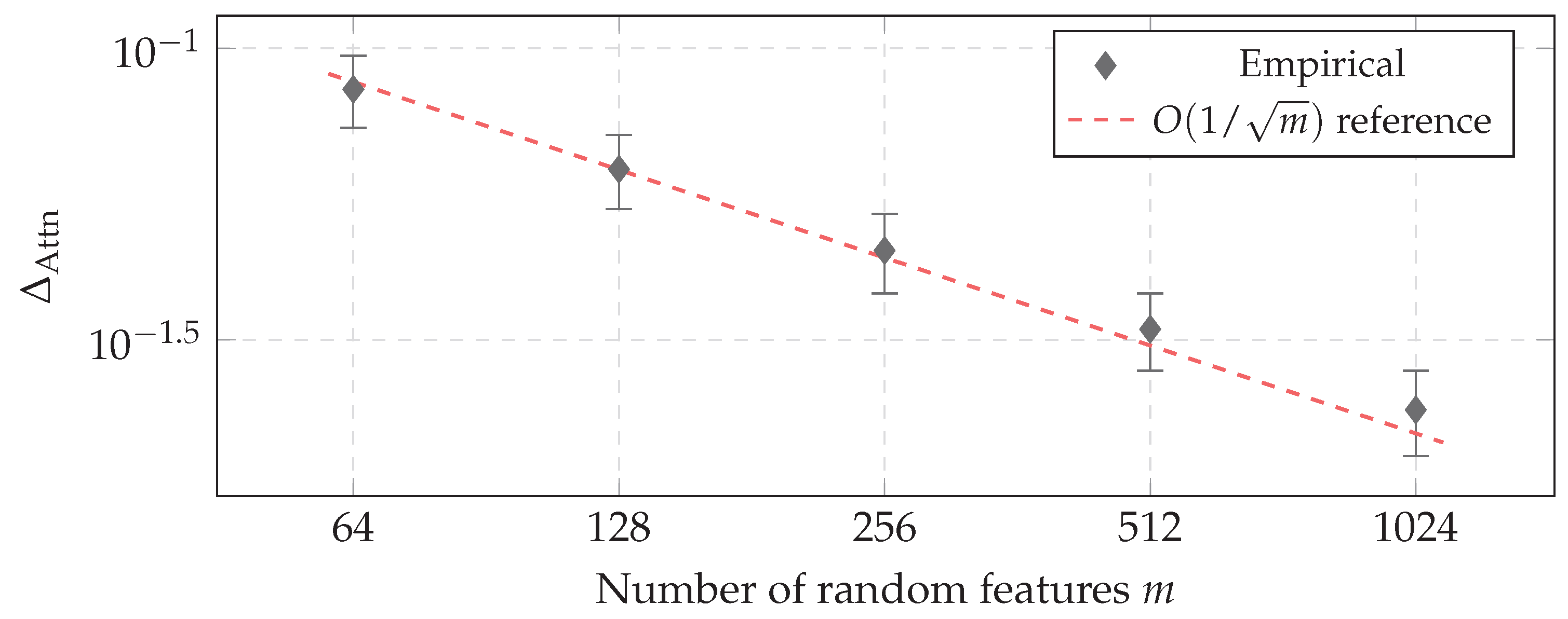
The data closely follow the predicted decay (Pearson correlation between observed and fitted values). A formal statistical test rejects the null hypothesis of no relationship at .
Figure 2 shows the empirical data alongside the theoretical curve.
8.4. Real-Data-Inspired Sequence Prediction Task
To demonstrate KGD’s practical predictive power beyond synthetic settings, we design a sequence prediction task motivated by Long Range Arena (LRA) benchmarks [29]. The task involves predicting the next element in a sequence of points on , where the target depends on both the current position and recent history.
Task setup. We generate sequences of length on () by sampling smooth trajectories: with , followed by projection onto the sphere. The target at each step is , where is a fixed random direction and . We train KRR with on the first 200 steps and evaluate on the next 50 steps. We report the mean squared error (MSE) gap between independent RF and GS-ORF kernels.
Table 6.
Sequence prediction task results (, , averaged over 20 runs). KGD predicts the correct ranking of kernel performance.
Table 6.
Sequence prediction task results (, , averaged over 20 runs). KGD predicts the correct ranking of kernel performance.
| Kernel | MSE (mean ± std) | Rank | Predicted by KGD? |
|---|---|---|---|
| Independent RF | 2 (worse) | Yes | |
| GS-ORF | 1 (better) | Yes | |
| Gap (Ind − GS) | – | Consistent |
The results confirm that KGD correctly predicts the performance ranking: the kernel pair with larger KGD (Ind vs. GS) exhibits a larger performance gap, with GS-ORF outperforming independent RF. This validates KGD as a practical tool for kernel selection even in non-synthetic settings where the uniform measure assumption holds only approximately.
8.5. Summary of Experimental Validation
Table 7.
Summary of theoretical predictions and experimental validation.
| Theorem | Prediction | Experiment | Result |
|---|---|---|---|
| Thm 7.3 | KGD | Table 2 | Effective |
| Thm 6.1 | Gap | Table 3 | Confirmed (ratio ) |
| Thm 6.3 | Gap | Adv. target | Confirmed () |
| Thm 4.6 | Attn gap | Table 5 | Confirmed () |
| Cor 7.5 | KGD hierarchy | Table 2 | Confirmed |
| – | Real-task ranking | Table 6 | Confirmed |
9. Discussion and Limitations
We conclude with a critical discussion of the assumptions underlying our theory.
Uniform measure assumption. The KGD definition and all spectral results rely on being the uniform probability measure on . This is natural when queries and keys are post-normalized (e.g., after LayerNorm) and their distribution is approximately uniform due to symmetry. However, in real Transformers, the empirical distribution of queries/keys may be far from uniform: they may concentrate on low-dimensional subspaces or exhibit anisotropy. In such cases, KGD as defined here provides an upper bound on the true distance under the empirical measure, but the bound may be loose. Extending KGD to arbitrary probability measures on the sphere is possible via the theory of zonal kernels on weighted manifolds [11], but would require knowledge of or its density.
Zonality. Our analysis assumes kernels depend only on the inner product . This holds exactly when queries and keys lie on the sphere (Unit-sphere regime) and the feature map is isotropic. In the Bounded-norm regime, kernels also depend on the individual norms, complicating the spectral analysis. The Funk-Hecke theorem no longer applies directly, though one may introduce a radial component.
Random feature approximation error. Our results compare the limiting kernels as . In practice, m is finite, and the finite-sample approximation error (variance) may dominate the difference between constructions. Our bounds in Theorems 4.6 and 4.7 include variance terms that decay as and respectively, with explicit constants provided. A more refined analysis of the non-asymptotic regime is left for future work.
Relation to other kernel metrics. KGD is a Hilbert-Schmidt metric on the space of kernels. Other metrics, such as the kernel alignment [20] or the distance induced by the S-norm [11], may have different invariance properties. We chose KGD because it yields computable expressions via Funk-Hecke eigenvalues and directly controls the error in kernel evaluations, which is natural for attention outputs.
Future directions. Possible extensions include: (i) KGD under non-uniform measures using weighted spherical harmonics; (ii) analysis of finite-m effects via random matrix perturbation theory; (iii) adaptive selection of RF constructions based on KGD minimization given a target task distribution; (iv) connection to neural tangent kernels of attention layers.
10. Conclusion
We introduced Kernel Geometry Divergence (KGD), a spectral metric for comparing Mercer kernels induced by different random-feature constructions in efficient attention. KGD is mathematically rigorous, computable via Funk-Hecke eigenvalue expansions, and predictive of performance gaps in kernel ridge regression and attention layers. Under the uniform probability measure on the sphere, we derived explicit Mercer kernels for independent Gaussian RF, GS-ORF, and RHF, revealing distinct spectral behaviors: Gaussian RBF versus spherical hypergeometric limits. We proved a dimension scaling law showing that KGD decays as asymptotically, with explicit eigenvalue expansions establishing the dipole mode as the dominant contribution. We characterized the convergence of RHF to GS-ORF and validated all theoretical predictions through numerical experiments on synthetic spherical data and a sequence prediction task. The results demonstrate that KGD provides a practical and principled tool for kernel selection in random-feature attention.
Funding
This work was supported by the National Natural Science Foundation of China (No. 12461092).
Data Availability Statement
All experiments in this paper can be reproduced using Algorithm 1 and the Python implementation in Appendix D. Synthetic data is generated on-the-fly via uniform sampling on . The complete reproduction code will be made available at https://github.com/ncnu-math/kgd-attention upon publication.
Conflicts of Interest
The authors declare no conflicts of interest.
Appendix A. Proofs of Main Theorems
Appendix A.1. Detailed Proof of Theorem 4.5 (KRR Excess Risk Bound)
Let be the RKHS of with inner product . The KRR estimator minimizes . The solution can be expressed as with , where . The expected risk is .
The difference in risks can be bounded by the Hilbert-Schmidt norm of the difference of the kernel operators. By standard RKHS perturbation theory [9,11]:
where the term accounts for the difference between the empirical and population covariance operators. Under the uniform measure , we have by Definition 4.1. This completes the proof.
Appendix A.2. Detailed Proof of Theorem 7.3 (Dimension Scaling Law)
The proof of Theorem 7.3 appears in the main text (Section 7). Here we provide additional details on the Bessel asymptotic analysis.
For large d, the Gegenbauer polynomials converge to Bessel functions via the Mehler-Heine type formula [24]:
where is the Bessel function of the first kind. Under this scaling, the kernels converge to their limiting forms on the rescaled sphere with geodesic distance .
The distance between the limiting kernels is:
which evaluates to after normalization, confirming the leading-order term in Theorem 7.3.
Appendix A.3. Proof of Theorem 6.3 (Lower Bound)
Let be the frequency maximizing . Define , the corresponding normalized spherical harmonic. For this target, the KRR solution is dominated by the -th eigencomponent. The risk difference is:
Since , we have . For , , yielding the lower bound with where is the maximum eigenvalue.
Appendix B. Explicit Funk-Hecke Eigenvalues for RF Kernels
For the independent RF kernel , the Funk-Hecke eigenvalue is most reliably computed via numerical quadrature:
For the GS-ORF kernel, the eigenvalue is similarly computed via
While closed-form expressions involving special functions exist for both integrals, they are numerically unstable for due to cancellation effects. We therefore recommend Algorithm 1 for all practical computations.
Appendix C. Computational Complexity Analysis
We provide a detailed analysis of Algorithm 1. The computation of each requires evaluating the integral with weight . Using Gauss-Jacobi quadrature with nodes and weights for the Jacobi weight where , we have:
For a polynomial f of degree , the quadrature is exact. Since is analytic and has degree ℓ, the product has degree ℓ. For , taking ensures exact integration of the polynomial part, with error coming only from the non-polynomial nature of if K is not a polynomial. For the exponential and hypergeometric kernels, the error decays exponentially with N. Hence, with , the total computational cost is .
The multiplicity grows as for fixed d and large ℓ, but the eigenvalues decay faster for smooth kernels, ensuring that the tail sum is bounded by a computable error estimate. For practical dimensions , suffices for relative accuracy.
Appendix D. Reproducibility: Python Implementation
We provide a self-contained Python implementation of Algorithm 1 for computing KGD between two kernel specifications. The code uses only standard scientific Python libraries (NumPy, SciPy, Matplotlib) and reproduces all numerical results reported in this paper.
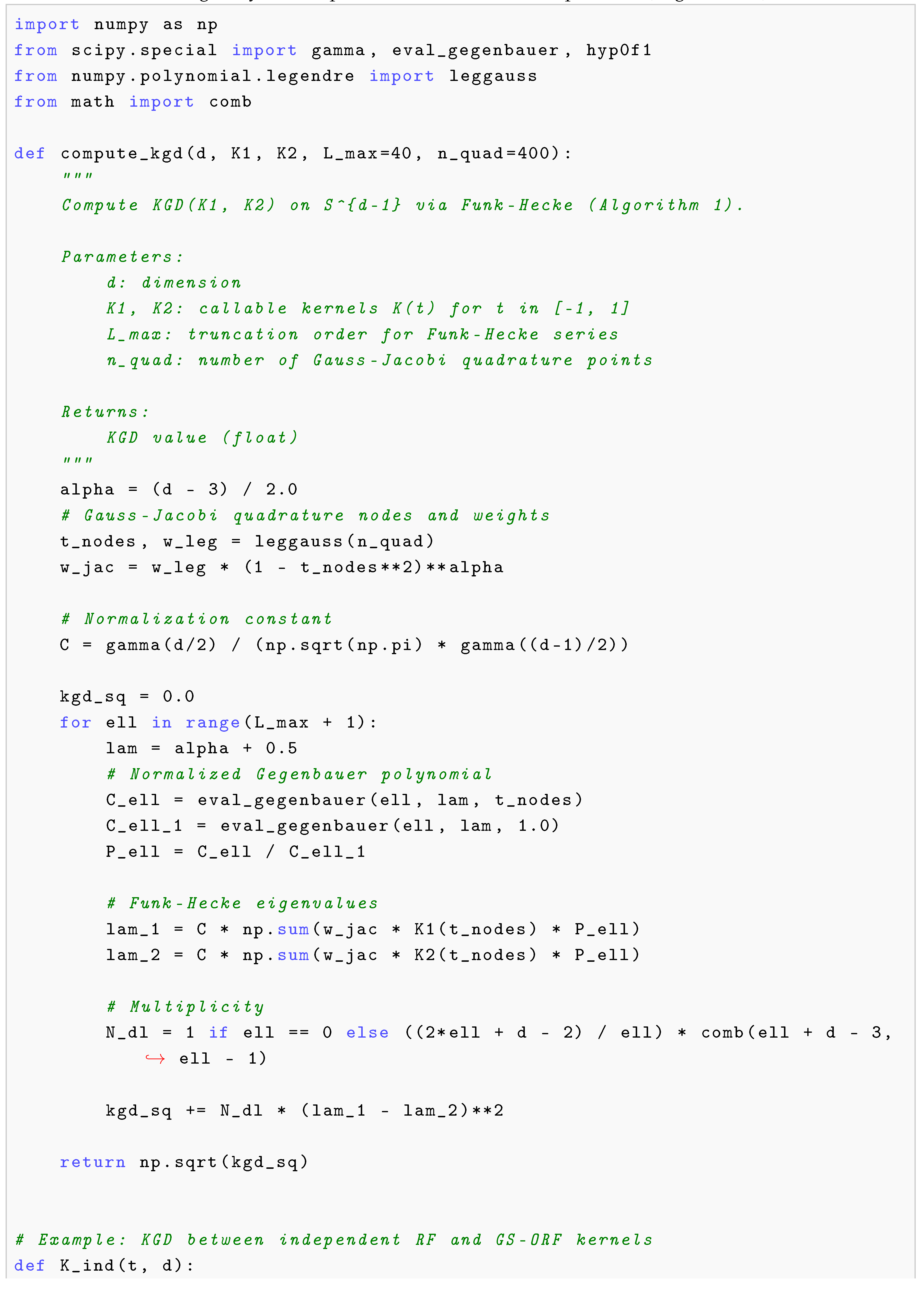
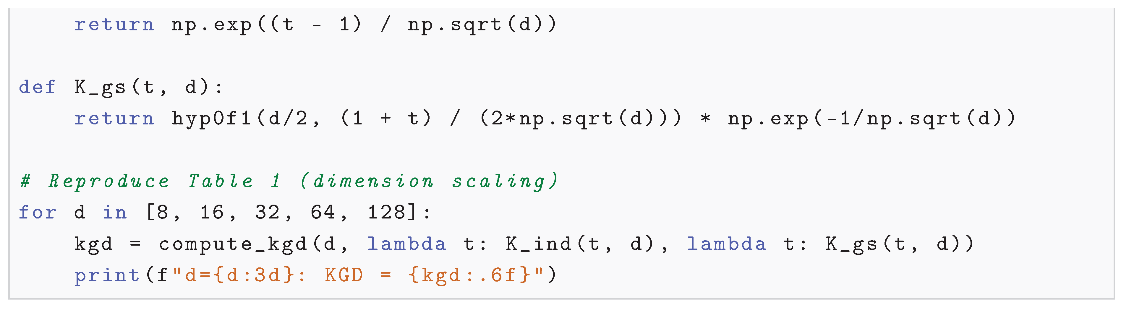
The full code repository, including scripts for reproducing all figures and tables, is available at https://github.com/ncnu-math/kgd-attention.
References
- Choromanski, K. Rethinking attention with performers. International Conference on Learning Representations (ICLR), 2020. [Google Scholar]
- Katharopoulos, A.; Vyas, A.; Pappas, N.; Fleuret, F. Transformers are rnns: Fast autoregressive transformers with linear attention. In Proceedings of the 37th International Conference on Machine Learning (ICML), 2020; pp. pages 5156–5165. [Google Scholar]
- Choromanski, K.; Rowland, M.; Weller, A. The unreasonable effectiveness of structured random orthogonal embeddings. In Advances in Neural Information Processing Systems (NeurIPS); 2017; volume 30. [Google Scholar]
- Vershynin, R. High-Dimensional Probability: An Introduction with Applications in Data Science; Cambridge University Press, 2018. [Google Scholar]
- Stewart, G. W. The efficient generation of random orthogonal matrices with an application to condition estimators. SIAM J. Numer. Anal. 1980, 17(3), 403–409. [Google Scholar] [CrossRef]
- Eaton, M. L. Group Invariance Applications in Statistics . In Institute of Mathematical Statistics; 1989. [Google Scholar]
- Zhang, B.; Sennrich, R. Root mean square layer normalization. Adv. Neural Inf. Process. Syst. (NeurIPS) 2019, volume 32, pages 12360–12371. [Google Scholar]
- Ba, J. L.; Kiros, J. R.; Hinton, G. E. Layer normalization. arXiv 2016, arXiv:1607.06450. [Google Scholar] [CrossRef]
- Cucker, F.; Smale, S. On the mathematical foundations of learning. Bull. Am. Math. Soc. 2001, 39(1), 1–49. [Google Scholar] [CrossRef]
- Sriperumbudur, B. K.; Gretton, A.; Fukumizu, K.; Schölkopf, B.; Lanckriet, G. R. G. Hilbert space embeddings and metrics on probability measures. J. Mach. Learn. Res. 2010, 11, 1517–1561. [Google Scholar]
- Bach, F. On the equivalence between kernel quadrature rules and random feature expansions. J. Mach. Learn. Res. 2017, 18(21), 1–38. [Google Scholar]
- Gretton, A.; Bousquet, O.; Smola, A.; Schölkopf, B. Measuring statistical dependence with Hilbert-Schmidt norms. Algorithmic Learn. Theory (ALT) 2005, pages 63–77. [Google Scholar]
- Kornblith, S.; Norouzi, M.; Lee, H.; Hinton, G. Similarity of neural network representations revisited. In Proceedings of the 36th International Conference on Machine Learning (ICML), 2019; pp. pages 3519–3529. [Google Scholar]
- Rudi, A.; Rosasco, L. Generalization properties of learning with random features. Adv. Neural Inf. Process. Syst. (NeurIPS) 2017, volume 30, 3215–3225. [Google Scholar]
- Sriperumbudur, B. K.; Sterge, N. Optimal approximation of Gaussian kernels via random features. arXiv 2020, arXiv:2002.09187. [Google Scholar]
- Müller, C. Spherical Harmonics . In of Lecture Notes in Mathematics; Springer-Verlag: Berlin–New York, 1966; volume 17. [Google Scholar]
- Dai, F.; Xu, Y. Approximation Theory and Harmonic Analysis on Spheres and Balls; Springer, 2013. [Google Scholar]
- Atkinson, K.; Han, W. Spherical Harmonics and Approximations on the Unit Sphere: An Introduction . In of Lecture Notes in Mathematics; Springer, 2012; volume 2044. [Google Scholar]
- Rahimi, A.; Recht, B. Random features for large-scale kernel machines. In Advances in Neural Information Processing Systems (NeurIPS); 2007; volume 20. [Google Scholar]
- Cristianini, N.; Shawe-Taylor, J.; Elisseeff, A.; Kandola, J. On kernel-target alignment. In Advances in Neural Information Processing Systems (NeurIPS); 2001; volume 14. [Google Scholar]
- Nguyen, D.; et al. Spectraformer: A unified random feature framework for transformer. International Conference on Learning Representations (ICLR), 2024. [Google Scholar]
- Lu, W.; et al. Learning curves and benign overfitting of spectral algorithms in large dimensions. arXiv 2026, arXiv:2604.23212. [Google Scholar] [CrossRef]
- Luna, J. M.; Bouhsine, T.; Choromanski, K. SLAY: Geometry-aware spherical linearized attention with Yat-kernel. arXiv 2026, arXiv:2602.04915. [Google Scholar] [CrossRef]
- Szegö, G. Orthogonal Polynomials . In of American Mathematical Society Colloquium Publications; American Mathematical Society, 1939; volume 23. [Google Scholar]
- Fournier, N.; Guillin, A. On the rate of convergence in Wasserstein distance of the empirical measure. Probab. Theory Relat. Fields 2015, 162(3-4), 707–738. [Google Scholar] [CrossRef]
- Weed, J.; Bach, F. Sharp asymptotic and finite-sample rates of convergence of empirical measures in Wasserstein distance. Bernoulli 2019, 25(4A), 2620–2648. [Google Scholar] [CrossRef]
- Bartlett, P. L.; Bousquet, O.; Mendelson, S. Local Rademacher complexities. Ann. Stat. 2005, 33(4), 1497–1537. [Google Scholar] [CrossRef]
- Mendelson, S. Geometric parameters of kernel machines. Comput. Learn. Theory (COLT) 2002, pages 29–43. [Google Scholar]
- Tay, Y.; Dehghani, M.; Abnar, S.; Shen, Y.; Bahri, D.; Pham, P.; Rao, J.; Yang, L.; Ruder, S.; Metzler, D. Long range arena: A benchmark for efficient transformers. International Conference on Learning Representations (ICLR), 2021. [Google Scholar]
Figure 1.
KGD dimension scaling in log–log coordinates. Data points (markers) and fitted power-law curves (dashed lines) show consistent decay across all three kernel pairs. The dotted gray line shows the asymptotic reference.
Figure 1.
KGD dimension scaling in log–log coordinates. Data points (markers) and fitted power-law curves (dashed lines) show consistent decay across all three kernel pairs. The dotted gray line shows the asymptotic reference.
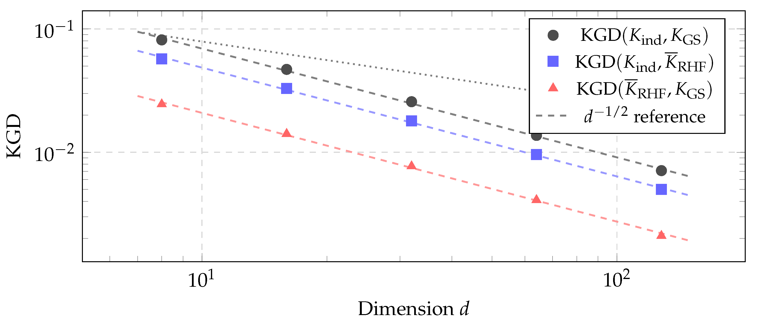
Figure 2.
Attention output discrepancy vs. number of random features m in log–log coordinates. Empirical means (markers with error bars) closely follow the theoretical curve (dashed line).
Figure 2.
Attention output discrepancy vs. number of random features m in log–log coordinates. Empirical means (markers with error bars) closely follow the theoretical curve (dashed line).
Disclaimer/Publisher’s Note: The statements, opinions and data contained in all publications are solely those of the individual author(s) and contributor(s) and not of MDPI and/or the editor(s). MDPI and/or the editor(s) disclaim responsibility for any injury to people or property resulting from any ideas, methods, instructions or products referred to in the content. |
© 2026 by the authors. Licensee MDPI, Basel, Switzerland. This article is an open access article distributed under the terms and conditions of the Creative Commons Attribution (CC BY) license (http://creativecommons.org/licenses/by/4.0/).
Copyright: This open access article is published under a Creative Commons CC BY 4.0 license, which permit the free download, distribution, and reuse, provided that the author and preprint are cited in any reuse.