

Submitted:
06 June 2026
Posted:
09 June 2026
You are already at the latest version
Abstract
Hepatitis B remains a major public health concern worldwide, particularly in developing nations where poor vaccination coverage, lack of screening, unsafe sexual practices, and delayed treatment fuel its spread. We developed a fractional-order model incorporating vaccination, screening, post-exposure prophylaxis (PEP), acute and chronic infection management, and behavioural measures. Theoretical analysis confirmed the model's existence, uniqueness, positivity, and boundedness. Equilibrium states were identified, and the basic reproduction number (R0) was derived via the next-generation matrix. The disease-free equilibrium is locally and globally asymptotically stable when R0< 1, while the endemic equilibrium exists and is globally asymptotically stable when R0>1. Model fitting and parameter estimation used acute Hepatitis B data from Ireland. Sensitivity analysis identified vaccination, screening, and safe practices as the most influential control factors. Numerical simulations showed that conventional strategies alone are insufficient; higher vaccination coverage, efficient screening, improved safe practices, and effective PEP are essential to reduce transmission. Collectively, these interventions minimize progression to chronic disease, reduce long-term burden, lower complications and mortality, particularly when acute infection management is included.
Keywords:
multi-level interventions
; safe practices
; post-exposure prophylaxis
; screening
; fractional-order model
1. Introduction
Hepatitis is a common deadly infectious disease caused by a viral infection that attacks and damages the liver cells (either temporarily or permanently) of a person. One serious type is Hepatitis B, which poses one of the highest threats to humans worldwide. Hepatitis B is caused by the hepatitis B virus (HBV), a member of the Hepatitis virus family that is enclosed. This DNA virus has a circular and partly double-stranded DNA genome. It replicates in the hepatocytes and disrupts normal liver functions, which in turn induces an immune response to produce an immune attack to fight or even clear the viral infection. The inflammation of the liver is due to pathology-caused damages [1,2].
In simple terms, Hepatitis B infects the liver and leads to degenerative changes such as cytolysis, fibrosis, and necrosis, and also induces hepatocellular inflammatory damage. The disease may present itself in acute and chronic forms over time [3]. However, certain percentages of infected individuals remain asymptomatic and may be carriers that can develop chronic infection in the future [4]. Chronic Hepatitis B is diagnosed when the virus is still detected six months after infection, indicating that the virus has not been cleared from the system [5]. After exposure, clinical symptoms may not appear for several weeks. When manifested, symptoms include yellowing of the skin and eyes (jaundice), dark urine, nausea, vomiting, diarrhea, and stomach discomfort [4,5,6].
Reports show that Hepatitis B can be transmitted early in a population. Transmission may be horizontal (contact between infectious individuals or contaminated objects and their body fluids/items) or vertical (from infected mother to baby) [7]. Furthermore, transmission routes differ significantly from the progression of the disease from latent to active infection [8]. Individuals who have undergone organ transplantation or have AIDS have a high probability of developing chronic infection after initial exposure, while infants less than six months old infected with the virus also have a high likelihood of developing chronicity [4].
Efforts to control the Hepatitis B public health threat have been recognized internationally over decades, with the aim of `elimination’ of the disease by 2030 [9]. The addition of a birth dose for the hepatitis B vaccination series is one of the best options to prevent vertical transmission of HBV from infected mothers to their infants [10]. The vaccine has been shown to effectively prevent HBV transmission; studies on Asian and Alaskan populations proved significant in population-wide infant/child vaccination programs [11,12].
Over half of all people living with Hepatitis B are not aware that they have been infected, and up to 50–70% of those with acute hepatitis B infection are asymptomatic [13]. Thus, if undiagnosed individuals are unable to know their status, continued transmission will occur from unknowingly infected individuals to unsuspecting victims [13]. Therefore, screening should be conducted for individuals who have a risk of exposure as long as that risk persists, regardless of age. This includes individuals with histories of sexually transmitted diseases, people who have sex with multiple partners, prison inmates, newborns of HBsAg-positive women, people with HIV, men who have sex with men [8], housemates of people diagnosed with HBV infection, and sex partners or needle sharers of infected individuals. PEP involves the use of medications administered to individuals exposed to HBV to prevent subsequent infection [13,14]. These at-risk groups may undergo PEP to avoid infection.
Mathematical models of infectious diseases are tools that assist in understanding and predicting disease transmission and assessing interventions. This study proposes a fractional-order model for the transmission of Hepatitis B, formulated based on fractional calculus, which emerged as the generalization of integer-order calculus [15]. Fractional-order models have played a substantial role in enhancing results associated with existing classical models [12]. This approach involves the use of nonlocal derivative operators [16].
There are many definitions of fractional derivatives; the most notable for disease modeling are Caputo, Caputo-Fabrizio, and Atangana-Baleanu, which incorporate memory effects [17]. Memory effects represent how a system’s current state is affected by its entire history, not just the immediate past [18]. This makes fractional models more effective for diseases with long incubation periods and long-lasting vaccine waning, such as Hepatitis B. Furthermore, the fractional system allows an infinite number of choices for the order of the derivative, unlike the integer order [19].
Although fractional-order HBV models have been developed in previous studies [6,12,15,16], they do not comprehensively incorporate the combined effects of vaccination, screening, PEP, acute infection management, chronic infection treatment, and safe practice adherence within a single framework. Specifically, [6] focused only on basic vaccination and fuzzy parameters without including screening, PEP, or behavioral interventions; [12] incorporated vaccination and age structure but omitted screening, PEP, and disease management; [15] examined asymptomatic carriers but lacked any clinical interventions; and [16] considered socio-environmental factors and awareness but did not include explicit screening, PEP, or treatment of acute and chronic infection. Furthermore, these existing models lack calibration to country-specific time-series data, such as acute Hepatitis B cases from Ireland, and do not fully assess how the collective impact of these interventions influences disease transmission and elimination thresholds. To address these gaps, this study develops a fractional-order Hepatitis B transmission model that integrates multi-level clinical interventions and behavioral measures, fitted to Irish data, to provide a more realistic tool for public health planning.
The remainder of this paper is organized as follows. Section 2 presents the methodology, which includes the preliminary concepts, model formulation, theoretical analysis, and model validation. Section 3 presents the numerical results. Section 4 provides a discussion of the results. Section 5 concludes the paper.
2. Materials and Methods
This study develops a fractional-order model to describe Hepatitis B dynamics under multi-level clinical control strategies, including vaccination, PEP, effective screening, acute infection management, chronic infection treatment, and compliance with safe practices (e.g., safe sex and personal hygiene). The model is formulated using fractional calculus, whose basic principles are briefly discussed. Boundedness and positivity of solutions are proved using the comparison theorem, while existence and uniqueness are established via the Banach fixed-point theorem. The disease-free equilibrium is obtained by setting all infected state variables to zero. The basic reproduction number is computed using the next-generation matrix approach. Local and global stability of the disease-free equilibrium are established using the Routh-Hurwitz criterion and the Castillo-Chavez method, respectively. The existence condition for the endemic equilibrium is determined using Descartes’ rule of signs.
2.1. Preliminary
2.1.1. Reimann-Liouville Fractional Integral
The Reimann Liouville fractional integral of a function of order is defined as
When , this becomes the standard (first-order) integral of .
2.1.2. Reimann-Liouville Fractional Derivative
Let such that . The Reimann Liouville fractional derivative of assumed to be n-times differentiable, is defined of ,
2.1.3. Caputo Fractional Derivative
Let such that . The Caputo fractional derivative of , assumed to be n-times differentiable, is defined as
In particular, if , it simplifies to
2.1.4. Laplace Transforms of Caputo Derivative
Let denoted the Laplace transform of . The Laplace transform of its Caputo derivatives is:
2.1.5. Mittag-Leffler Functions
The one-parameter Mittag-Leffler function is defined as
2.1.6. Inverse Laplace Transform of Caputo derivative
The inverse Laplace transform is used to retrieve the original function. A fundamental result is the following inverse transform, which yields the Mittag-Leffler function:
2.2. Model Formulation
The whole population is divided into multiple epidemiological compartments according to infection state and intervention status, incorporating both clinical and behavioural intervention effects. The compartments include Susceptible (S), Exposed (E), Acutely infected (A), Chronically infected (C), Screened (Q), Recovered (R), and Vaccinated (V). New members enter the susceptible population through birth and immigration at a constant rate .
The transition from susceptible to exposed occurs when susceptible individuals come into effective contact with infectious populations (either acutely or chronically infected). The transmission rate depends on the force of infection , which incorporates effective behavioural compliance that reduces risky contacts due to behavioural interventions (e.g., safe sex practices with condom usage, avoidance of syringe sharing, etc.).
The exposed class represents individuals in the incubation stage of Hepatitis B infection, which has several biologically plausible pathways for further progression. Screening is applied at rate with effectiveness ; screened individuals may qualify for prophylactic treatment (PEP) and progress to the vaccinated class at rate if treatment is successful, or move to the acutely infected population at rate . However, some exposed individuals may be detected early or develop chronic infection without passing through the acute infection stage, or due to asymptomatic nature hepatitis B, some unscreened infected may progress directly from exposed to chronic stage at rate .
The acutely infected stage reflects an active infection that will either progress to chronic infection or result in recovery. Clinical management is modeled as parameter with effectiveness , promoting recovery by increasing the recovery rate and slowing the progression to the chronic stage.
Chronic infected individuals serve as the reservoir of infection in the community. Entry into the chronic stage occurs through direct transition from exposed or acutely infected individuals at rate . Individuals in the chronic stage may die due to infection at rate . Recovered and vaccinated individuals gain permanent immunity. All compartments are subject to natural death at rate . The compartment dynamics and transitions are shown in Figure 1, and the Caputo fractional-order nonlinear system is given in equation (9).
For
The state variables and parameters of the model are summarized in Table 1.
2.3. Boundedness of the Solution
Theorem 1.
The solution of system (9) is feasible for all if they enter the invariant region in the absence of the disease-induced mortality rate
Proof.
Consider the total population so that;
Substituting the right-hand side of the equations in the system (9) and simplifying, (10) reduced to a linear fractional-order differential equation (11).
since , it follows that:
applying (6) to (12) we get;
applying (8) to (15) we get;
clearly, as .
Thus, .
Therefore, the total population is bounded. Each compartment is also bounded if we can show that all compartments are non-negative. □
2.4. Positivity of the Solution
Theorem 2.
Let the initial data be , then the solution of system (9) is remain non-nagetive for all .
Proof.
Consider the first equation of the system (9) that is;
Applying the same procedure to rest of the equations of (9), we obtained the following non-negative solutions;
□
To conclude the proof of existence and uniqueness for the solution of (9), we establish existence in Appendix A and prove Theorem 3.
Theorem 3.
The fractional order system (9) of hepatitis B has a unique solution if
Proof.
Since have an upper bound, and the kernel satisfies Lipschitz, then (A6) gives
Clearly, as . with this result, the existence of a solution for the fractional order hepatitis B model (9) is established.
To show the uniqueness, consider two solutions S and S, satisfying the first equation of (9) then
Hence, the proof of Theorems 1, 2.4, and 3, together with the uniqueness of the solution established in Appendix A, completes the proof of existence, boundedness, and uniqueness of the solution. □
2.5. Disease-Free Equilibrium (DEF)
The disease-free equilibrium is the state in which no individuals in the population are infected. That is, all infectious classes and recovery are zero. That is, but and . So,
Thus, following disease-free equilibrium points are obtained by setting the derivative of non-zero compartments (S and V ) to zero.
2.6. Basic Reproduction Number
The basic reproduction number (, is a crucial threshold parameter for modelling infectious diseases. It is referred to as the number of secondary infections produced by a single hepatitis B infected individual in a population that is fully susceptible to the disease. If , then the infection will die out, while if implies the disease will persist in the soceity. The basic reproduction number is computed using the method discussed in [11,12,22] and detailed in [23,24].
Let represent the vector of infected compartments, then;
where F and V are Jacobian matrices of and evaluated at DEF respectively.
where and ,
The critical reproduction number is given by the spectral radius . The reproduction number is called the critical (or effective) reproduction number when controls are present.
Thus,
By setting all control parameters to zero — specifically, the vaccination rate , vaccination efficacy , post-exposure prophylaxis (PEP) rate , screening rate , treatment rates and the effectiveness parameters — the model reduces to its baseline form with no interventions. Under this condition, the basic reproduction number is obtained as:
This expression represents the expected number of secondary infections generated by a single infected individual introduced into a completely susceptible population in the absence of any public health interventions.
The basic reproduction number can be decomposed into two contributions:
- Direct chronic contribution:, arising from exposed individuals who progress directly to the chronic state.
- Acute-mediated contribution:, arising from exposed individuals who progress first to the acute state and then to the chronic state.
Both terms are scaled by ,
where is the average duration in the Exposed compartment, is the average duration in the Acute compartment, and is the average infectious period for chronic carriers.
2.7. Local Stability of Disease-Free Equilibrium
Theorem 4.
The disease-free equilibrium (DFE) is locally asymptotically stable (LAS) if all the eigenvalues of the Jacobian matrix of (9) evaluated at disease-free equilibrium satisfy: when otherwise unstable.
The proof of the theorem is provided in Appendix B. From a biological perspective, the theorem implies that when the reproduction number is below one, the introduction of a small number of infected individuals into an otherwise HBV-free population will not lead to an outbreak. Instead, the infection will gradually decline and the population will return to the disease-free state over time.
2.8. Global Stability of Disease-Free Equilibrium
The disease-free equilibrium (DFE) is said to be globally asymptotically stable if the system returns to this equilibrium point regardless of the initial infection levels. The Castillo-Chavez [25] method is used to show the global stability of the fractional-order hepatitis B model (9).
Theorem 5.
The disease-free equilibrium of the system (9) is globally asymptotically stable if Otherwise unstable.
The proof of the theorem is provided in Appendix C. Biologically, this implies that the incidence of Hepatitis B can be controlled regardless of the initial number of infected individuals, even in the midst of a large outbreak, provided the basic reproduction number remains below unity. In other words, the disease-free equilibrium is globally asymptotically stable when .
2.9. Existence of Endemic Equilibrium
When hepatitis B infection is present in the population, the system (9) has an endemic equilibrium point denoted by . And by equating Where the right hand sides of (9) to zero, the following endemic equilibrium points are obtained.
if , then .
So,
The force of infection is expressed as
substituting (33), (34), and (37) into (38) and simplifying, we obtain
where
It is obvious that (39) has a zero root which indicates the existence of stable disease-free equilibrium. If , (39) has a positive root. That is, there is an endemic equilibrium. Consequently, we claimed the following theorem
Theorem 6.
In the absence of control, the endemic equilibrium of the system (9) exists and is unique if and only if .
2.10. Model Validation and Parameter Estimation
Estimates of model parameters were achieved by fitting to time-series data on acute hepatitis B cases obtained from [27] for 20 years (2004–2024) in Ireland. Other population records (such as total population, average life expectancy, etc.) for the country were obtained from [28]. A non-linear least squares method was used for the fitting. To allow the model to effectively reproduce the actual dynamics of hepatitis B transmission, appropriate initial parameter guesses help the optimisation algorithm (Trust-Region-Reflective) towards optimal parameter values. For realistic fitting, parameter bounds are imposed so that the estimated parameters remain in the biologically feasible region.
Figure 2 shows the observed acute hepatitis B cases and the fitted model output over the period 2004–2024. The fitted values (solid blue line) closely track the observed data (solid red circles), capturing the initial peak in 2004, the subsequent decline, and the stabilisation at lower levels in recent years. This close agreement indicates that the model adequately reproduces the transmission dynamics.
Figure 3(a) presents the residual plot, which exhibits random scatter around zero with no systematic pattern, suggesting no significant model misspecification. Figure 3(b) shows the Q-Q plot of the residuals, where the points approximately follow the theoretical diagonal line, supporting the normality assumption. Figure 3(c) presents the box plot, showing that the predicted data closely match the observed data in terms of median, quartiles and range, with no extreme outliers.
The corresponding statistics for the observed and predicted data, including the mean, , RMSE and other summary measures, are summarised in Table 2. These diagnostic checks collectively validate the goodness-of-fit of the proposed model.
The fitted and estimated parameters are summarised in Table 3.
3. Results
The fractional-order system (9) was solved numerically using the Adams-Bashforth-Moulton method with the parameter values listed in Table 1. The section is organised into subsections, each presenting figures relevant to the dynamics under consideration. Further details of the numerical simulation results are given in Section 4 (Results and Discussion).
3.1. Global Convergence
To verify the global stability of the equilibria, numerical simulations were performed using multiple distinct initial conditions for the infected compartments. Specifically, we varied the initial numbers of exposed, acute and chronic individuals to assess whether the system converges to the same equilibrium regardless of the starting point.
Figure 4(a)–Figure 4(f) and Figure 5(a)–Figure 5(b) illustrate that all infected compartments converge to the disease-free equilibrium (DFE) irrespective of the initial infected population size. This behaviour is consistent with the theoretical global stability condition , confirming that the infection dies out over time even when introduced at high levels.
3.2. Sensitivity Analysis
Sensitivity analysis determines the influence of each model parameter on disease transmission, helping to identify which aspects should be the primary focus of intervention strategies as they significantly affect [29,30]. The normalised sensitivity index for a parameter p is defined as:
- indicates that an increase in p increases .
- indicates that an increase in p decreases .
From Table 4, the most influential parameters are , and , which positively affect , while , and have strong negative effects, reducing . The positive indices for and indicate that screening alone, without effective post-screening isolation or treatment, does not reduce disease transmission. In the model, screened individuals either receive PEP (moving to the vaccinated class) or progress to acute and then chronic infection. Thus, screening merely channels exposed individuals through pathways that still lead to chronic infection. This emphasized the necessity of pairing screening with effective follow-up interventions such as PEP to lower .
3.3. Memory Effect
To assess the memory effect on the system, we simulate the compartments at various fractional orders and compare the results with the integer-order case (), as shown in Figure 9(a)–Figure 9(f). The fractional-order parameter captures the memory inherent in biological systems, where past infections and immunity influence future transmission dynamics. Lower values of indicate a stronger memory effect, leading to slower decays and more persistent dynamics compared to the memoryless integer-order case.
3.4. Impact of Vaccination
Figure 10(a) shows the impact of vaccination on the susceptible compartment. As the vaccination rate increases, the susceptible population declines more rapidly, reflecting the protective effect of vaccination. Conversely, the vaccinated compartment increases with higher vaccination rates, as shown in Figure 10(b). This demonstrates that vaccination effectively reduces the pool of susceptible individuals and builds immunity in the population.
3.5. Impact of Screening
3.6. Impact of Safe Practice
3.7. Impact of Post-Exposure Prophylaxis
Post-exposure prophylaxis (PEP) reduces the progression of screened individuals to the acute or chronic compartments. Figure 13(a) demonstrates that as the PEP rate increases, the number of screened individuals declines because they are successfully treated. Consequently, the vaccinated compartment grows with higher PEP rates, as shown in Figure 13(b), indicating that PEP effectively moves individuals from the screened class to the protected vaccinated class.
3.8. Impact of Effective Management of Acute Infection
Effective management of acutely infected individuals enables recovery without progression to the chronic stage. Figure 14(a) and Figure 14(b) show that the recovery rate increases with higher management effectiveness . Figure 14(c) indicates that progression from acute to chronic infection can be minimised with proper management. As effectiveness increases, the progression rate decreases, as shown in Figure 14(d). To further demonstrate that effective management improves recovery, the recovery compartment is studied at different recovery rates (Figure 14(e)) and various levels of management effectiveness (Figure 14(f)).
3.9. Impact of Treatment of Chronic Infection
4. Discussion
In this study, a fractional-order mathematical model was developed to investigate the dynamics of Hepatitis B virus transmission, incorporating multi-level clinical interventions and safe practice adherence. The theoretical analysis established the existence, uniqueness, positivity, boundedness and well-posedness of the model. The basic reproduction number was computed using the next-generation matrix approach. It was shown that the disease-free equilibrium is locally and globally asymptotically stable when , while the endemic equilibrium exists and is globally asymptotically stable when .
Model fitting was performed using acute Hepatitis B case data from Ireland spanning 20 years (2004–2024), with parameter estimation achieved via the nonlinear least squares method. The fitting plot, box plot, residual plot and Q-Q plot of the residuals were presented alongside the summary statistics of the observed and predicted data. These diagnostic checks collectively confirm that the model effectively reproduces the actual transmission dynamics of Hepatitis B in Ireland.
Sensitivity analysis revealed that the contact rate , vaccination rate , PEP rate , progression rate , screening rate and screening effectiveness are the most influential parameters affecting the critical reproduction number . Notably, while screening ( and ) showed positive sensitivity indices, this counterintuitive result arises because screened individuals in the model are not isolated or treated; they merely progress through alternative pathways that still lead to chronic infection. This underscores the critical public health insight that screening must be paired with effective follow-up interventions such as treatment or isolation to achieve meaningful reductions in transmission.
Numerical simulations verified the analytical conclusions regarding the global stability of equilibria. The results demonstrated that each compartment converges to the disease-free equilibrium regardless of whether a small or large number of infected individuals is introduced, confirming the global asymptotic stability of the DFE when .
The impact of vaccination showed that as the vaccination rate increases, the susceptible compartment declines more rapidly while the vaccinated compartment grows correspondingly. Effective screening was shown to reduce progression to chronic infection, although without post-screening interventions, transmission potential may remain unchanged. Safe practices significantly reduced disease transmission, with higher compliance rates leading to greater reductions, even under high transmission rate conditions.
Effective PEP administration reduced progression of screened individuals to acute or chronic infection. As the PEP rate increases, the screened population declines while the vaccinated population increases. Proper management of acute infection () enabled recovery without progression to the chronic stage, with higher effectiveness increasing recovery rates and minimising chronic progression. Treatment of chronically infected individuals () reduced the endemic equilibrium level and increased recovery over time.
To assess the memory effect inherent in the fractional-order system, simulations were performed at various fractional orders and compared with the integer-order case (). Lower values of , corresponding to stronger memory effects, resulted in slower epidemic progression and delayed convergence to equilibrium. This demonstrates that fractional-order modelling captures the long-term memory effects of disease progression and intervention outcomes more accurately than integer-order models, particularly for a disease like Hepatitis B with long incubation periods and chronic persistence.
Compared to existing fractional-order HBV models, our study provides several advances. Unlike [6] and [12], which focused primarily on vaccination without screening or PEP, our results show that combining vaccination with screening, PEP and safe practices achieves a greater reduction in . Unlike [15], which examined asymptomatic carriers without interventions, our model demonstrates that multi-level interventions can control disease spread despite the presence of asymptomatic carriers. Unlike [16], which emphasised behavioural factors but lacked clinical interventions, our findings reveal that adding screening, PEP and treatment significantly lowers chronic infection burden beyond behavioural measures alone. Additionally, to the best of our knowledge, this study is the first to calibrate a fractional-order HBV model to country-specific time-series data (Ireland) and to assess the collective impact of all these interventions on disease elimination thresholds.
5. Conclusions
Hepatitis B remains a significant public health concern worldwide, particularly in developing nations where poor vaccination coverage, lack of screening programmes, unsafe practices and delayed treatment contribute substantially to disease spread and progression. This study successfully developed a fractional-order Hepatitis B transmission model incorporating vaccination, screening, PEP, acute infection management, chronic infection treatment and safe practice compliance. The theoretical and numerical results collectively demonstrate that multi-level clinical interventions and behavioural measures are essential for effective disease control.
The key findings of this study are as follows. Vaccination is the most influential parameter for reducing , with higher coverage accelerating the decline of susceptible individuals and enhancing herd immunity. Screening, while beneficial for reducing progression to chronic infection, requires follow-up interventions such as treatment, PEP or isolation to effectively lower transmission potential. Safe practice compliance significantly reduces transmission, even under high transmission rate conditions. PEP administration reduces progression to acute and chronic stages while increasing the vaccinated population. Proper acute infection management enhances recovery and minimises progression to the chronic stage. Chronic infection treatment reduces the endemic equilibrium level and increases recovery over time. Furthermore, the fractional-order approach captures memory effects, providing a more realistic representation of Hepatitis B dynamics than integer-order models.
Conventional control strategies alone may not be sufficient for mitigating Hepatitis B. Higher vaccination coverage, efficient screening programmes paired with follow-up interventions, improved adherence to safe practices, effective PEP administration and proper management of acute and chronic infections are essential for reducing disease transmission. These interventions collectively minimise progression to the chronic stage and its long-term burden, reduce the risk of Hepatitis B-induced complications such as cirrhosis and hepatocellular carcinoma, and lower disease-induced mortality.
The model has certain limitations. Parameter estimation relied on data from Ireland, and generalisability to other settings requires further validation. The model assumes homogeneous mixing and does not consider spatial heterogeneity or population structure. Future work should extend the model to include age structure, stochastic effects and cost-effectiveness analysis of the proposed intervention strategies.
Author Contributions
Conceptualization, N.A., A.A.U., Y.U.A. and M.A.; methodology, N.A., A.A.U, Y.U.A and M.A.; software, A.A.U. and Y.U.A.; validation, A.A.U., and M.A.; formal analysis, A.A.U.; investigation, N.A. and Y.U.A; resources, N.A.; data curation, A.A.U.; writing—original draft preparation, A.A.U.; writing—review and editing, N.A. and Y.U.A.; visualization, N.A. and A.A.U.; supervision, Y.U.A. All authors have read and agreed to the published version of the manuscript.
Funding
This research received no external funding.
Data Availability Statement
The data used in this work can be accessed in the work.
Acknowledgments
The author would like to thank the Deanship of Graduate Studies and Scientific Research, Taif University for providing resources and facilities that supported this work.
Conflicts of Interest
The authors declare no conflicts of interest.
Abbreviations
The following abbreviations are used in this manuscript:
| PEP | Post-exposure prophylaxis |
| HBV | Hepatitis B |
| DNA | Deoxyribonucleic acid |
| DFE | Disease-free equilibrium |
| EE | Endemic equilibrium |
| RMSE | Root mean square error |
Appendix A. Existence and Uniqueness of the Solution
The existence and uniqueness of the solution of (9) is established by employing the well-known Banach fixed-point theorem [20,21], which is also known as the contraction principle. Let be a Banach space of continuous real-valued function defined on the interval and with the norm
such that
,
Let where be the right-hand side of the system (9). That is,
Applying the Caputo fractional integral to both sides of (9), the following system of integral equations is obtained.
It is important to note that the kernel satisfies the Lipschitz condition if and only if has upper bounds. Consider two functions S and S, so that;
Following the same procedure, we obtained the following
where
With initial condition; , the difference between the successive terms gives the following
Let us consider.
Appendix B. Proof of Theorem 4
Proof.
The Jacobian matrix of the system (9) is evaluated at disease-free equilibrium as follows
And the eigenvalues of (A8) are
All the eigenvalues (A10) of the Jacobian matrix of the system (9) are negative real (with no imaginary part) in the disease-free state. except
Now, consider which the fourth and positive eigenvalue of (A8)
Obviously, if .
Since all the parameters are positive, then
Thus, if
Then
From equation 28, it can be clearly seen that if
So,
Therefore, all the eigenvalues satisfy: for , □
Appendix C. Proof of Theorem 5
The fractional-order system (9) can be expressed in the form;
where with representing hepatitis B uninfected and infected population, respectively.
To prove theorem (5), the system (9) must satisfy the following two conditions as in [25]:
is Metzler (all off-diagonal entries are non-negative).
- First Condition
We show that the non-infected classes S and V are stable
Applying (6) and (8) to (A14), we obtained the following solution
Obviously,
Clearly, S and V return to disease free equilibrium as time goes.
- Second Condition
where A is a Jacobian matrix of .
so, we obtain as follows;
since all the off-diagonal entries are non-negative, then A is Metzler
At disease-free, . But in the presence of disease, . Thus, .
Obviously, the second condition is also satisfied. Therefore. The disease-free equilibrium is globally asymptotically stable if □
References
- World Health Organization. Global hepatitis report 2024: action for access in low- and middle-income countries. 2024. Available online: https://www.who.int/publications/i/item/9789240091672.
- World Health Organization. Hepatitis B (WHO/CDS/CSR/LYO/2002.20). 2002. Available online: https://apps.who.int/iris/handle/10665/67746.
- Agnes, D. T.; Mayanna, H.; Abduraman, A. M. O.; et al. Hematological Profile of Patients with Hepatitis B Aged 18 To 60 Years. Clin. Immunol. Res. 2025, 9(1), 1–4. [Google Scholar] [CrossRef]
- Zada, I.; Naeem Jan, M.; Ali, N.; Alrowail, D.; Sooppy Nisar, K.; Zaman, G. Mathematical analysis of hepatitis B epidemic model with optimal control. Adv. Differ. Equ. 2021, 2021(1), 451. [Google Scholar] [CrossRef]
- Opoku, M.O.; Wiah, E.N.; Okyere, E.; Sackitey, A.L.; Essel, E.K.; Moore, S.E. Stability Analysis of Caputo Fractional Order Viral Dynamics of Hepatitis B Cellular Infection. Math. Comput. Appl. 2023, 28(24). [Google Scholar] [CrossRef]
- Mpeshe, S. C. Fuzzy fractional derivative model to assess the dynamics of hepatitis B infection. Eur. J. Math. App. 2023, 3, 17. [Google Scholar] [CrossRef]
- Asandem, D.A.; Segbefia, S. P.; Kusi, K. A.; Bonney, J. H. K. Hepatitis B Virus Infection: A Mini Review. Viruses 2024, 16, 724. [Google Scholar] [CrossRef] [PubMed]
- Li, C.; Wei, C.; Yang, X. Hepatitis B virus: modes of transmission, immune pathogenesis, and research progress on therapeutic vaccines. Explor Dig. Dis. 2024, 3, 443–58. [Google Scholar] [CrossRef]
- Mirgichan, J. K.; Ngari, C.G.; Karanja, S.; Murigichan, R. Mathematical modeling and simulation of hepatitis B transmission dynamics with passive immunity and control strategies. Heliyon 2025, 11(2). [Google Scholar] [CrossRef]
- Nelson, N. P.; Easterbrook, P. J.; Brian, J. Epidemiology of Hepatitis B Virus Infection and Impact of Vaccination on Disease. Clin. Liver Dis. 2016, 20(4), 607–628. [Google Scholar] [CrossRef]
- Abdulrahman, S.; Tech, M.; Akinwande, N. I.; Awojoyogbe, O. B.; Abubakar, U. Y. Mathematical Analysis of the Control of Hepatitis B Virus in a Population with Vital Dynamics. Pac. J. Sci. Technol. 2013, 14(1), 188–204. [Google Scholar]
- Tilahun, T. D.; Woldegerima, A. W.; Mohammed, N. A fractional order model for the transmission dynamics of hepatitis B virus with two-age structure in the presence of vaccination. Arab J. Basic Appl. Sci. 2021, 28:1, 87–106. [Google Scholar] [CrossRef]
- Centers for Disease Control and Prevention. Clinical testing and diagnosis for hepatitis B. 31 January 2025. Available online: https://www.cdc.gov/hepatitis-b/hcp/diagnosis-testing/index.html.
- Senoo-Dogbey, E. V.; Ohene, A. L.; Wuaku, A. D. Occupational exposure to Hepatitis B virus, disease burden and pathway for post-exposue prophylaxis management: recommendations for healthcare workers in highly endemic settings. Infect. Prev. Pract. 2024. [Google Scholar] [CrossRef]
- Gul, N.; Bilala, R.; Algehyne, A. E.; Alshehri, G. M.; Khan, A. M.; Chu, Y.; Islam, S. The dynamics of fractional order Hepatitis B virus model with asymptomatic carriers. Alex. Eng. J. 2021, 60(4), 3945–3955. [Google Scholar] [CrossRef]
- Sinha, A. K.; Soni, K. Fractional-order modeling of hepatitis B dynamics incorporating socio-environmental factors. In Discover Public Health; 2025. [Google Scholar] [CrossRef]
- Akuka, P. N.; Seidu, B.; Okyere, E.; Abagna, S. Fractional-Order Epidemic Model for Measles Infection. Scientifica 2024, 2024(1), 8997302. [Google Scholar] [CrossRef]
- Bhole, M. K.; Patil, M. D.; Vyawahare, V. A. Stability Analysis of Fractional-order Systems. International Conference & Workshop on Recent Trends in Technology, (TCET). ICWET2012, March 2012; 2012; 11, pp. 12–18. [Google Scholar]
- Qureshi, S.; Yusuf, A.; Shaikh, A. A.; Inc, M.; Baleanu, D. Fractional modeling of blood ethanol concentration system with real data application. Chaos An Interdiscip. J. Nonlinear Sci.> 2019, 29(1), 013143. [Google Scholar] [CrossRef]
- Ahmed, I.; Kiataramkul, C.; Muhammad, M.; Tariboon, J. Existence and sensitivity analysis of a Caputo fractional-order diphtheria epidemic model. Mathematics 2024, 12(13), 2033. Available online: https://www.mdpi.com/2227-7390/12/13/2033#. [CrossRef]
- Addai, E.; Ngungu, M.; Omoloye, M. A.; Marinda, E. Modelling the impact of vaccination and environmental transmission on the dynamics of monkeypox virus under Caputo operator. Math. Biosci. Eng. 2023, 20(6), 10174–10199. Available online: https://www.aimspress.com/article/doi/10.3934/mbe.2023446. [CrossRef]
- Mustapha, U. T.; Ahmad, Y. U.; Yusuf, A.; Qureshi, S.; Musa, S. S. Transmission dynamics of an age-structured Hepatitis-B infection with differential infectivity. Bull. Bio-Math. 2023, 1(2), 124–152. [Google Scholar] [CrossRef]
- Van den Driessche, P.; Watmough, J. Reproduction numbers and sub-threshold endemic equilibria for compartmental models of disease transmission. Math. Biosci. 2002, 180(1-2), 29–48. [Google Scholar] [CrossRef] [PubMed]
- Fosu, O. G.; Akweittey, E.; Adu-Sackey, A. Next-generation matrices and basic reproductive numbers for all phases of the Coronavirus disease. Open J. Math. Sci. 2020, 4, 261–272. [Google Scholar] [CrossRef]
- Castillo – Chavez, C.; Song, B. Dynamical Models of Tuberculosis and their Applications. Math. Bio-Sci. Eng. 2004, 1(2), 361–404. [Google Scholar] [CrossRef]
- Wodajo, A. F.; Gebru, M. D.; aAlemneh, T. H. Mathematical model analysis of effective intervention strategies on transmission dynamics of hepatitis B virus. Int. J. Res. Publ. Rev. 2023, 4(6). [Google Scholar] [CrossRef]
- Health Service Executive-Health Protection Surveillance Centre. Epidemiology of hepatitis B in Ireland: Trends up to 2024. 2025. Available online: https://www.hpsc.ie/a-z/hepatitis/hepatitisb/surveillancereports/Epidemiology%20of%20Hepatitis%20B%20in%20Ireland%20-%20June%202025_Final.pdf.
- World Bank. Ireland. World Bank Data. n.d. Available online: https://data.worldbank.org/country/ireland.
- Rodrigues, H. S.; Monteiro, T.T.; Torres Delfim, F. M. Sensitivity Analysis in a Dengue Epidemiological Model. Conf. Pap. Math. 721406 2013, 7 pages. [Google Scholar] [CrossRef]
- Rathee, S.; Narwal, Y.; Bansal, K. Sensitivity analysis of fractional order SVEIR Lumpy Skin Disease model. Alex. Eng. J. 2025, 119 609–622. [Google Scholar] [CrossRef]
Figure 1.
Schematic diagram of the Hepatitis B model described in equation (9), showing the flow between compartments.
Figure 1.
Schematic diagram of the Hepatitis B model described in equation (9), showing the flow between compartments.
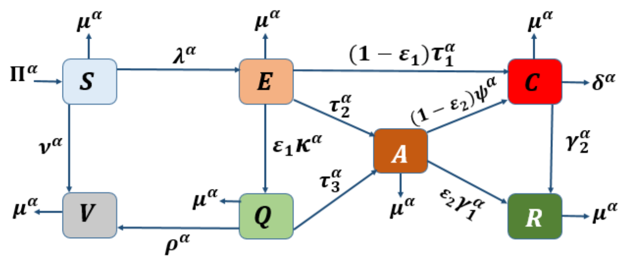
Figure 2.
Description of the acute class A fitted to real-data: The observed data points closely follow the predicted line.
Figure 2.
Description of the acute class A fitted to real-data: The observed data points closely follow the predicted line.
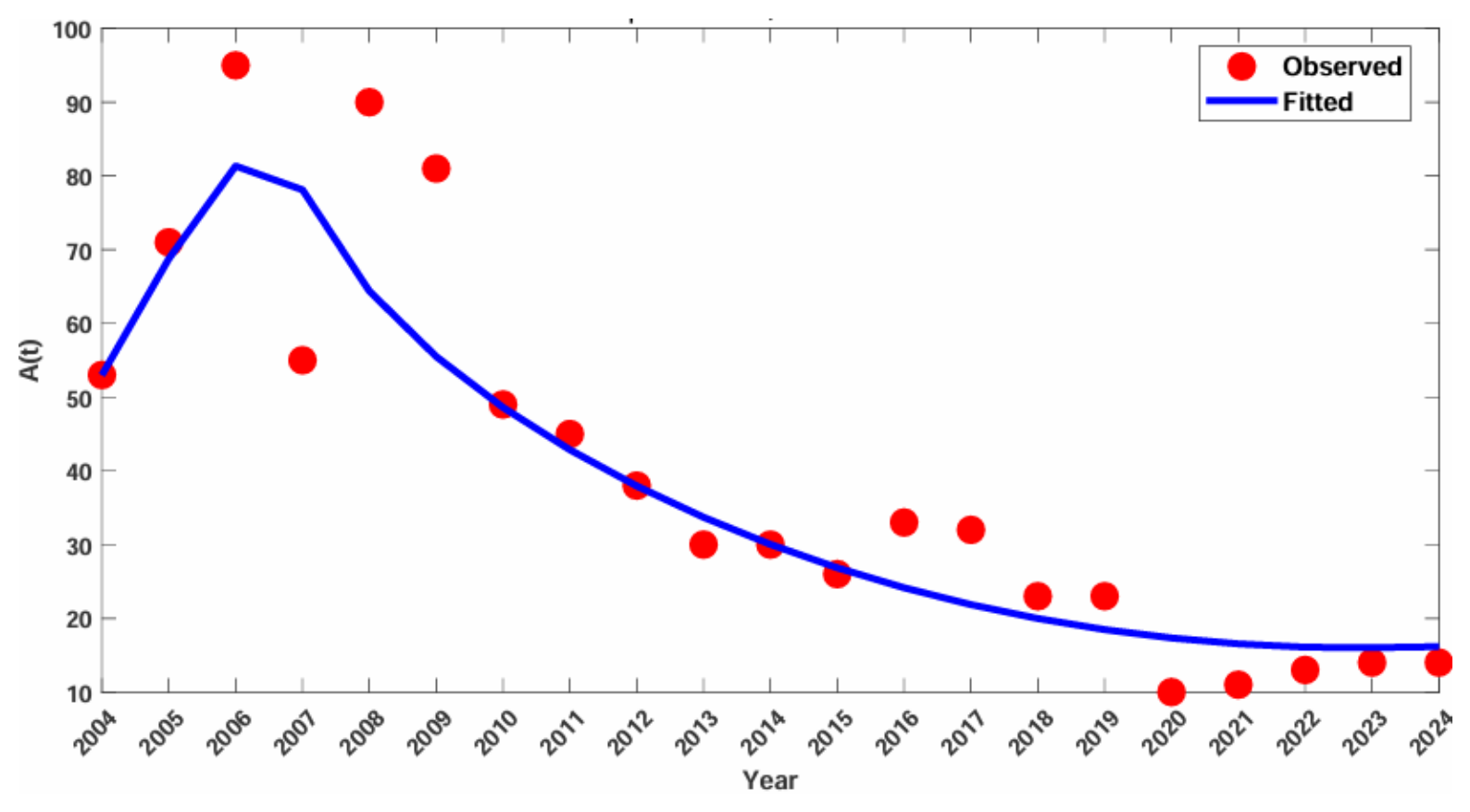
Figure 3.
(a) Description of the residual plot: Random scatter with constant variance. (b) Description of the QQ plot of the residuals: Good fit to the normality line. (c) Description of the box plot of the residuals: Symmetric with no outliers.
Figure 3.
(a) Description of the residual plot: Random scatter with constant variance. (b) Description of the QQ plot of the residuals: Good fit to the normality line. (c) Description of the box plot of the residuals: Symmetric with no outliers.
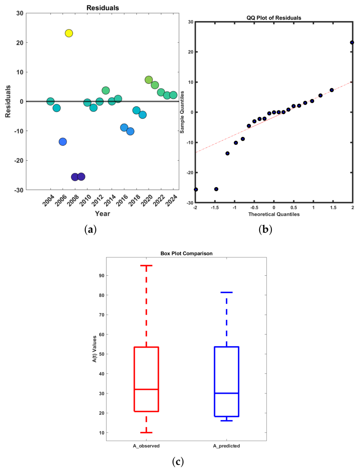
Figure 4.
Description of the global convergence of the infection to the DFE. Panels: (a,b) show the Exposed class. (c,d) show the Screened Exposed class. (e,f) show the Acute class. Within each pair, the two panels differ only by the initial number of infections.
Figure 4.
Description of the global convergence of the infection to the DFE. Panels: (a,b) show the Exposed class. (c,d) show the Screened Exposed class. (e,f) show the Acute class. Within each pair, the two panels differ only by the initial number of infections.
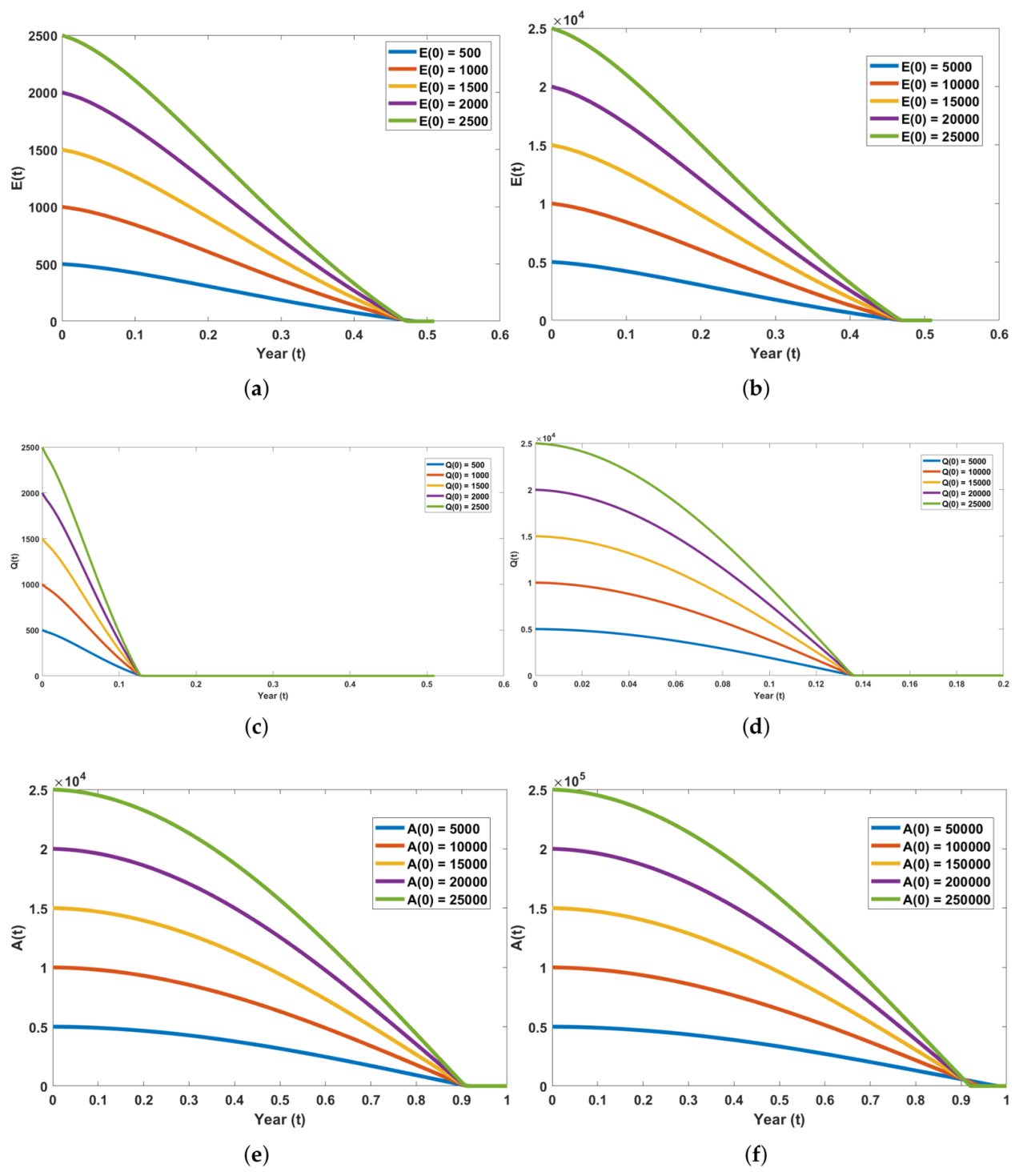
Figure 5.
Description of the global convergence of the infection. Panels: (a,b) show the Chronic class converging to the DFE. (c,d) show the Exposed class converging to the EE. (e,f) show the Screened Exposed class converging to the EE. Within each pair, the two panels differ only by the initial number of infections.
Figure 5.
Description of the global convergence of the infection. Panels: (a,b) show the Chronic class converging to the DFE. (c,d) show the Exposed class converging to the EE. (e,f) show the Screened Exposed class converging to the EE. Within each pair, the two panels differ only by the initial number of infections.
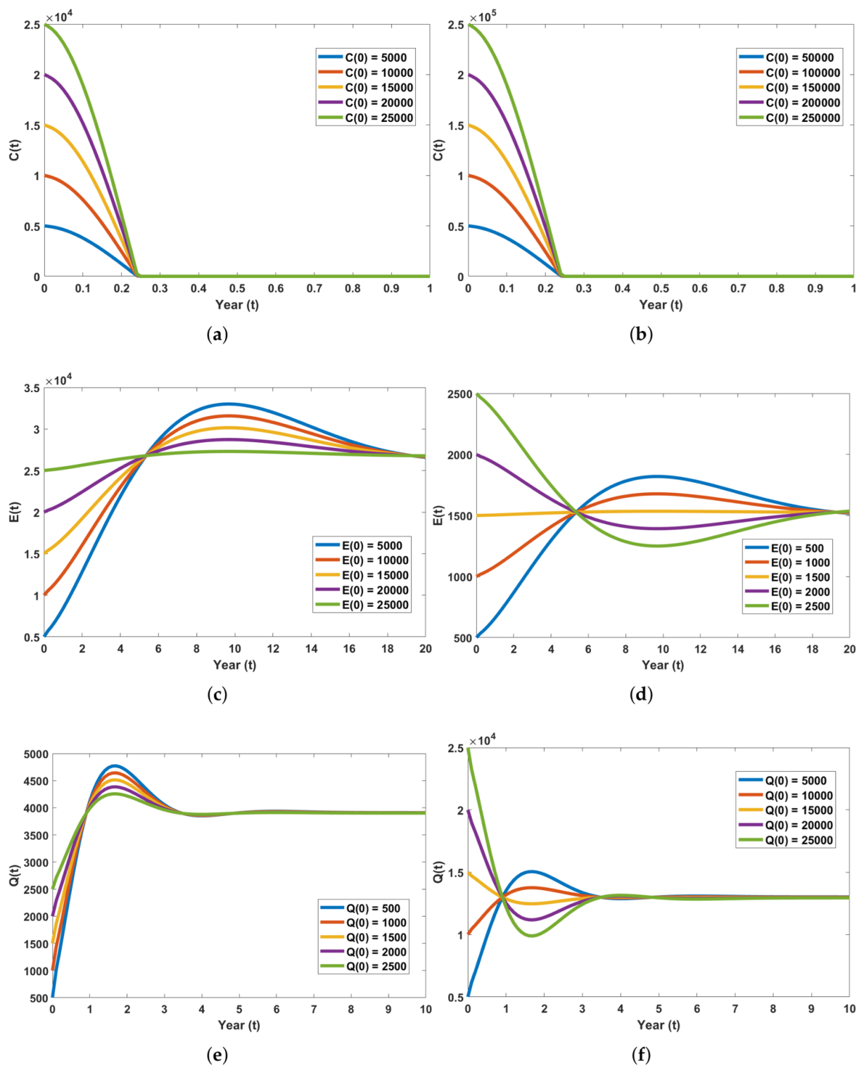
Figure 6.
Description of the global convergence of the infection to the EE. Panels: (a,b) show the Acute class. (c,d) show the Chronic class.
Figure 6.
Description of the global convergence of the infection to the EE. Panels: (a,b) show the Acute class. (c,d) show the Chronic class.
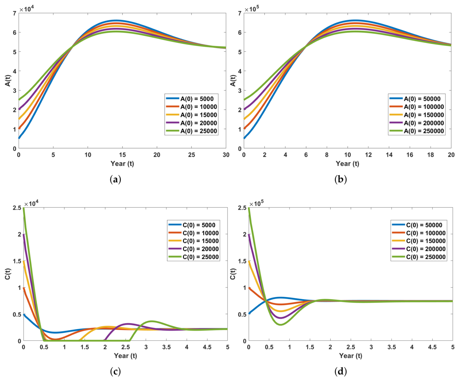
Figure 7.
(a) Description of the bar plot of sensitivity indices for the dominant parameters. (b) Description of the bar plot of sensitivity indices for the near-zero parameters.(c) Description of the 2D contour plot of vaccination rate and contact rate versus the control reproduction number. (d) Description of the 3D contour plot of vaccination rate and contact rate versus the control reproduction number.
Figure 7.
(a) Description of the bar plot of sensitivity indices for the dominant parameters. (b) Description of the bar plot of sensitivity indices for the near-zero parameters.(c) Description of the 2D contour plot of vaccination rate and contact rate versus the control reproduction number. (d) Description of the 3D contour plot of vaccination rate and contact rate versus the control reproduction number.
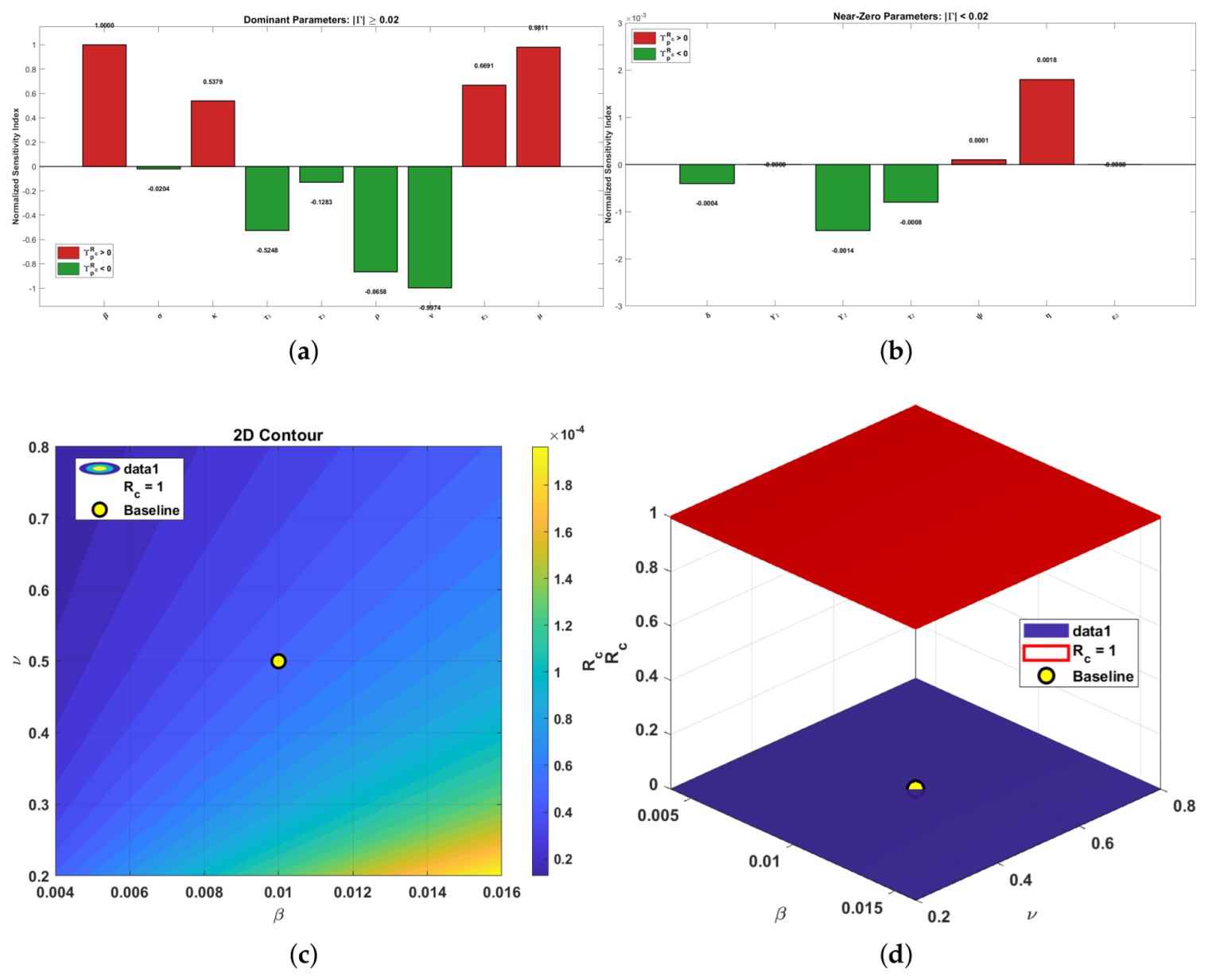
Figure 8.
(a) Description of the 2D contour plot of screening effectiveness and safe practice compliance rate versus control reproduction number. (b) Description of the 3D contour plot of screening effectiveness and safe practice compliance rate versus control reproduction number. (c) Description of the 2D contour plot of PEP rate and chronic infection modification parameter versus the control reproduction number. (d) Description of the 3D contour plot of PEP rate and chronic infection modification parameter versus the control reproduction number.
Figure 8.
(a) Description of the 2D contour plot of screening effectiveness and safe practice compliance rate versus control reproduction number. (b) Description of the 3D contour plot of screening effectiveness and safe practice compliance rate versus control reproduction number. (c) Description of the 2D contour plot of PEP rate and chronic infection modification parameter versus the control reproduction number. (d) Description of the 3D contour plot of PEP rate and chronic infection modification parameter versus the control reproduction number.
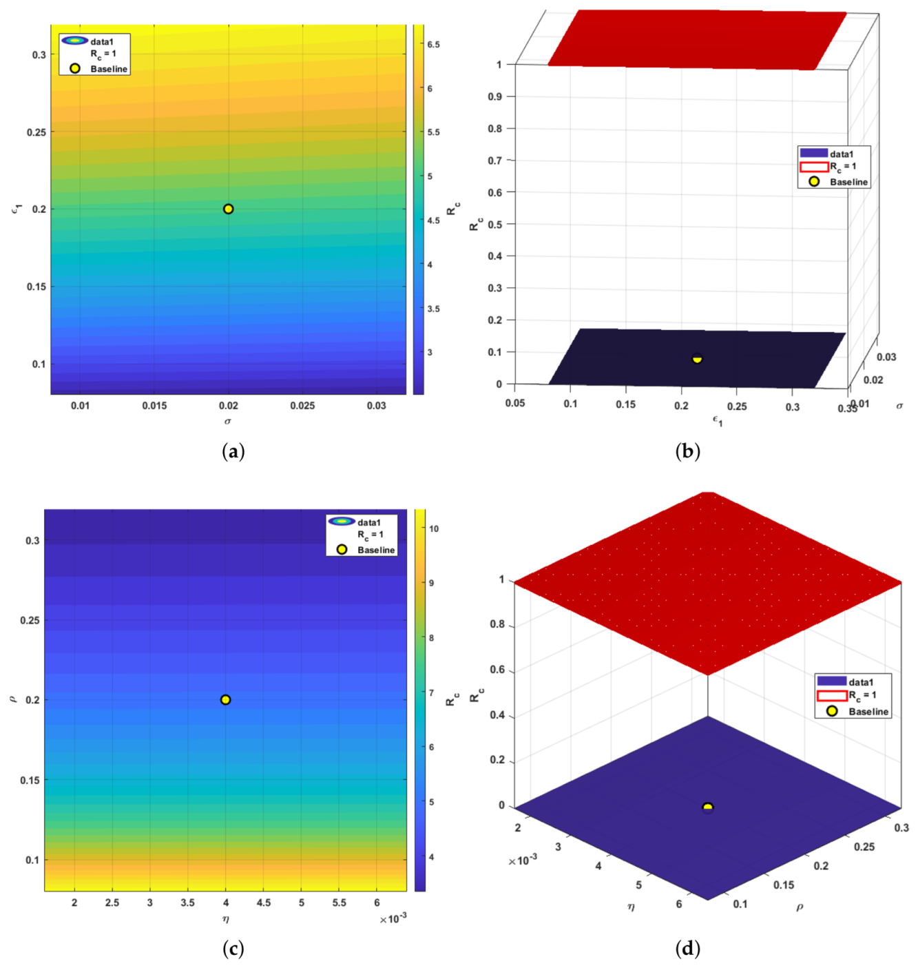
Figure 9.
Description of the memory effect on compartment dynamics: (a) Susceptible. (b) Exposed. (c) Screened Exposed. (d) Acute. (e) Chronic. (f) Vaccinated.
Figure 9.
Description of the memory effect on compartment dynamics: (a) Susceptible. (b) Exposed. (c) Screened Exposed. (d) Acute. (e) Chronic. (f) Vaccinated.
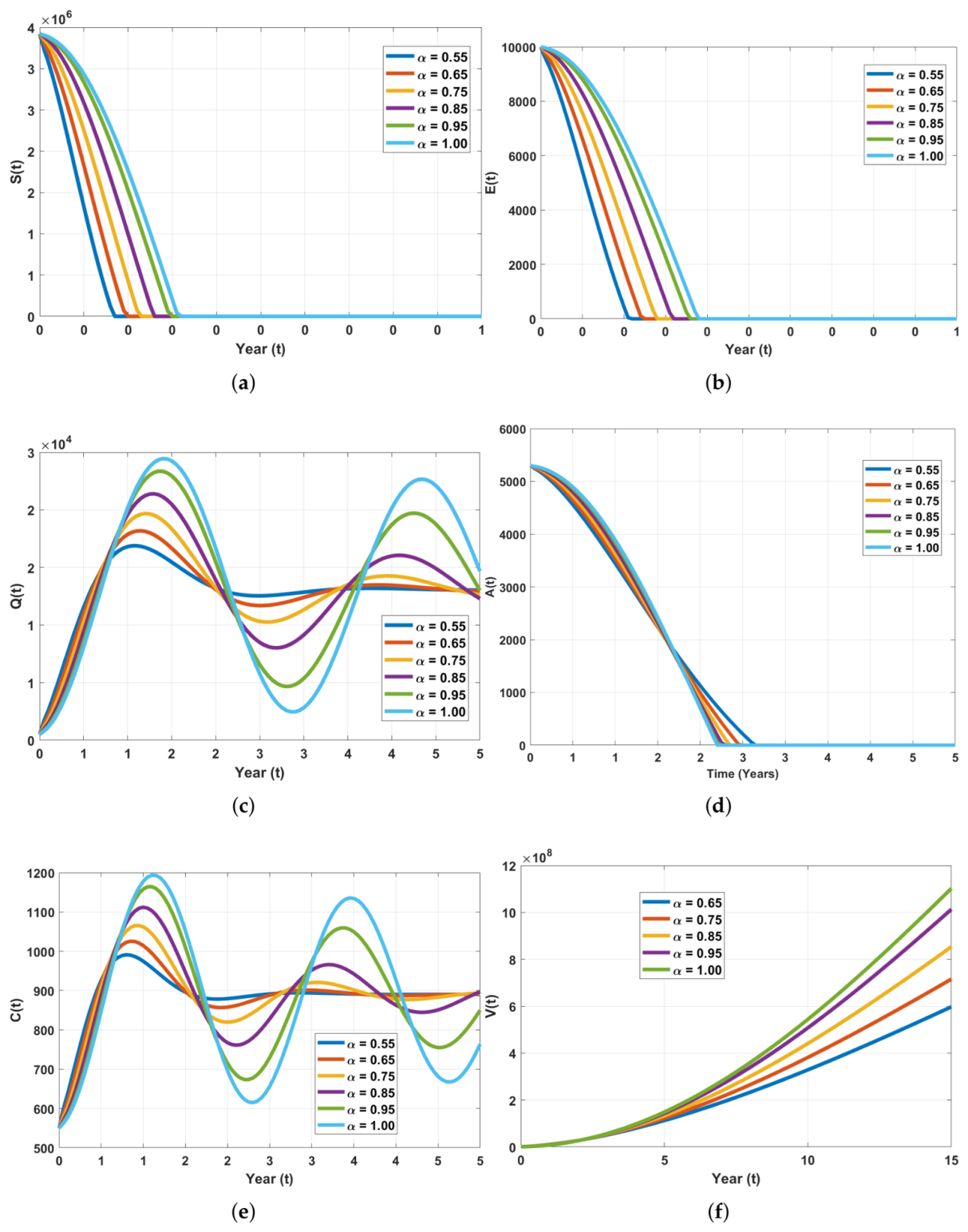
Figure 10.
Description of the impact of vaccination on the (a) Susceptible and (b) Vaccinated compartments.
Figure 10.
Description of the impact of vaccination on the (a) Susceptible and (b) Vaccinated compartments.
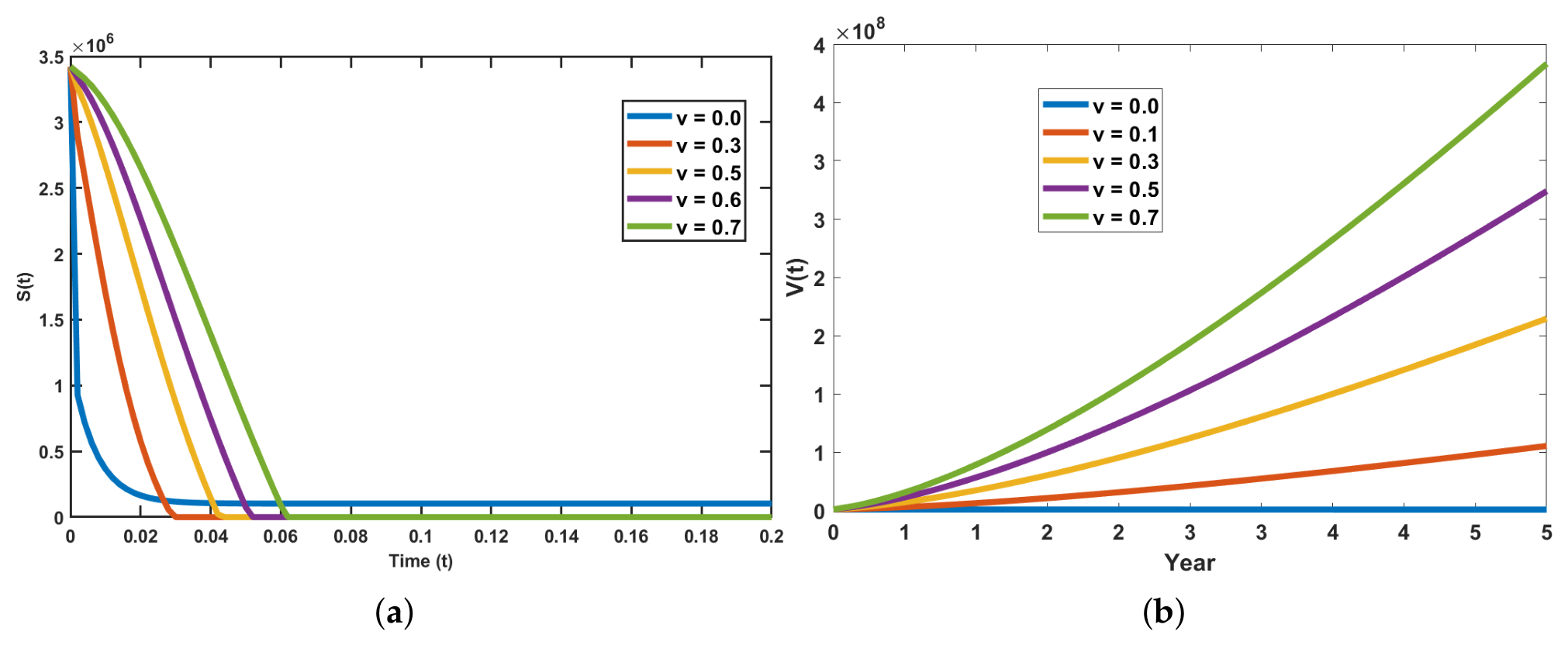
Figure 11.
(a) Impact of screening on the Exposed compartment. (b) Impact of screening effectiveness on the Exposed compartment. (c) Impact of screening effectiveness on the Chronic compartment with a small number of initial infections. (d) Impact of screening effectiveness on the Chronic compartment with a large number of initial infections.
Figure 11.
(a) Impact of screening on the Exposed compartment. (b) Impact of screening effectiveness on the Exposed compartment. (c) Impact of screening effectiveness on the Chronic compartment with a small number of initial infections. (d) Impact of screening effectiveness on the Chronic compartment with a large number of initial infections.
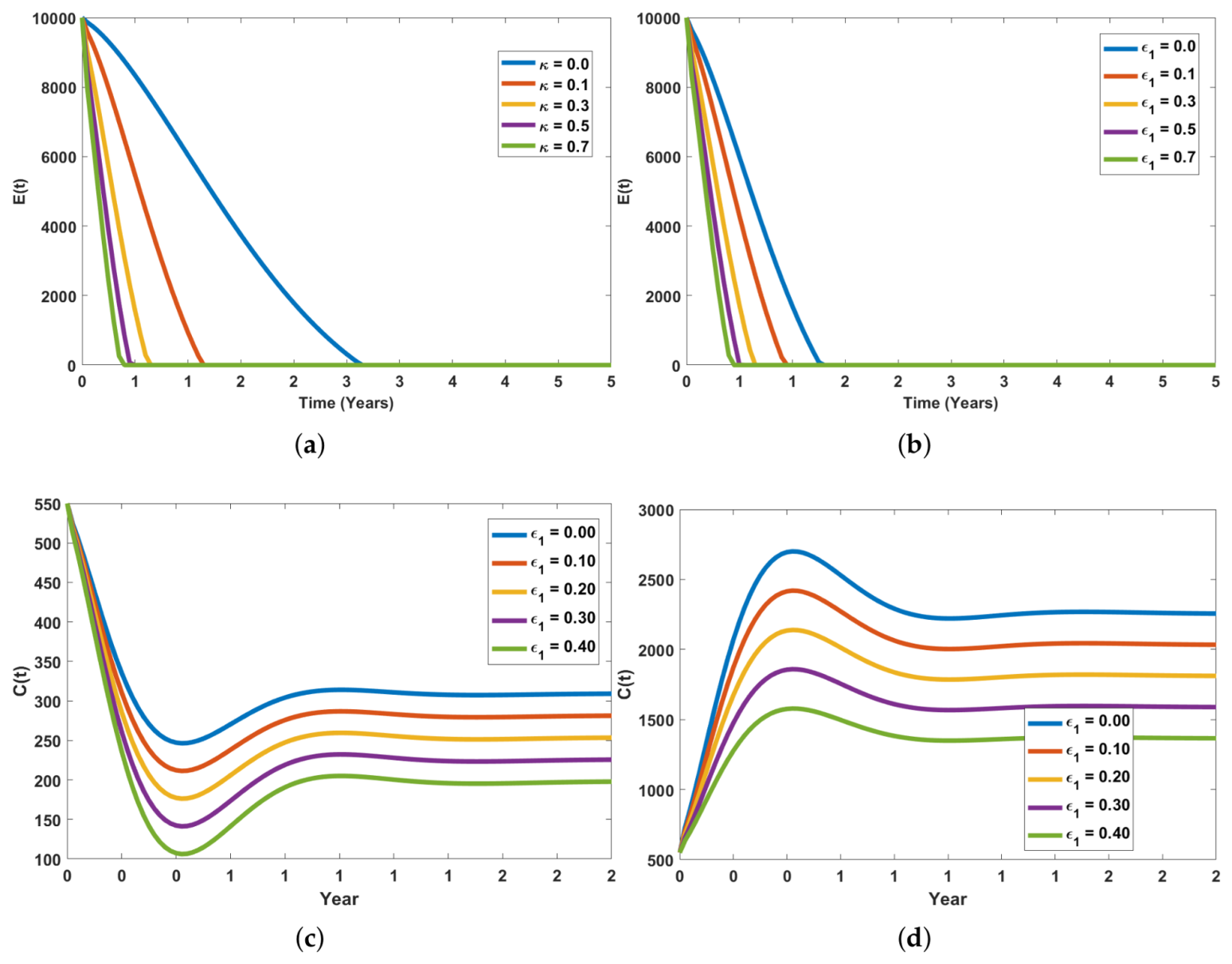
Figure 12.
(a) Safe practice compliance impact: Exposed compartment (low transmission rate). (b) Safe practice compliance impact: Exposed compartment (high transmission rate).
Figure 12.
(a) Safe practice compliance impact: Exposed compartment (low transmission rate). (b) Safe practice compliance impact: Exposed compartment (high transmission rate).
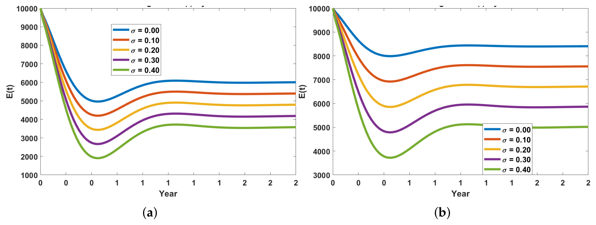
Figure 13.
(a) Impact of PEP on the Screened compartment. (b) Impact of PEP on the Vaccinated compartment.
Figure 13.
(a) Impact of PEP on the Screened compartment. (b) Impact of PEP on the Vaccinated compartment.
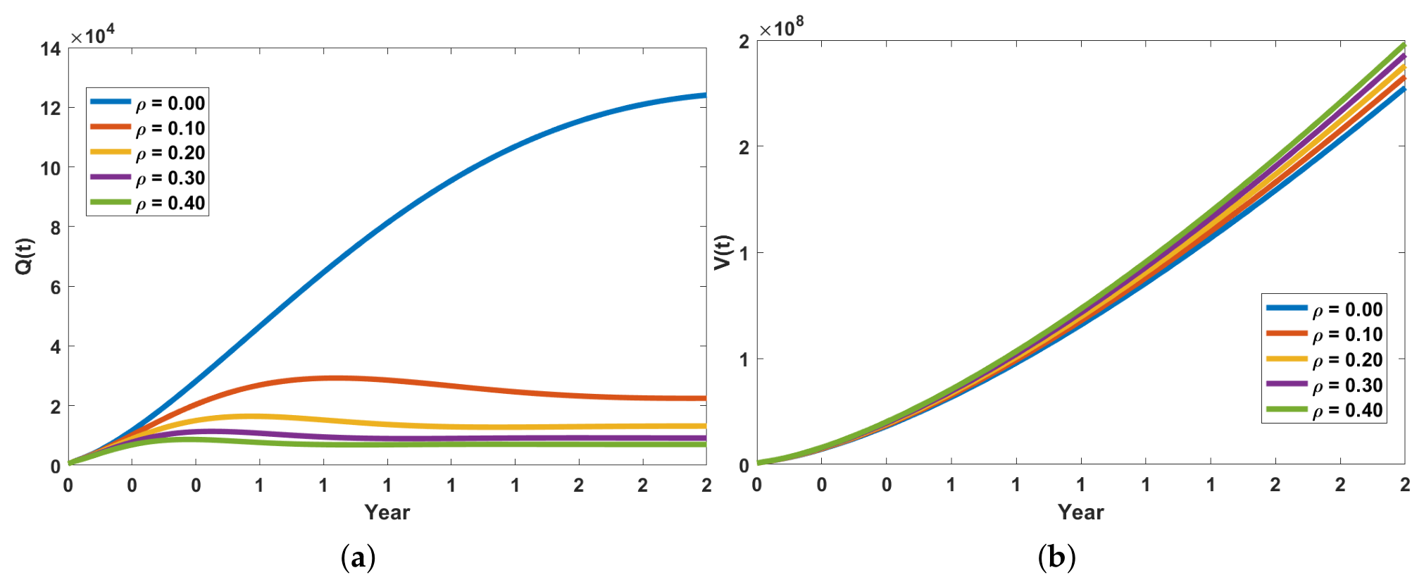
Figure 14.
(a) Impact of acute infection management on the Exposed compartment. (b) Effectiveness of acute infection management on the Exposed compartment. (c) Impact of acute infection management on the Chronic compartment. (d) Effectiveness of acute infection management on the Chronic compartment. (e) Impact of acute infection management on the Recovered compartment. (f) Effectiveness of acute infection management on the Recovered compartment.
Figure 14.
(a) Impact of acute infection management on the Exposed compartment. (b) Effectiveness of acute infection management on the Exposed compartment. (c) Impact of acute infection management on the Chronic compartment. (d) Effectiveness of acute infection management on the Chronic compartment. (e) Impact of acute infection management on the Recovered compartment. (f) Effectiveness of acute infection management on the Recovered compartment.
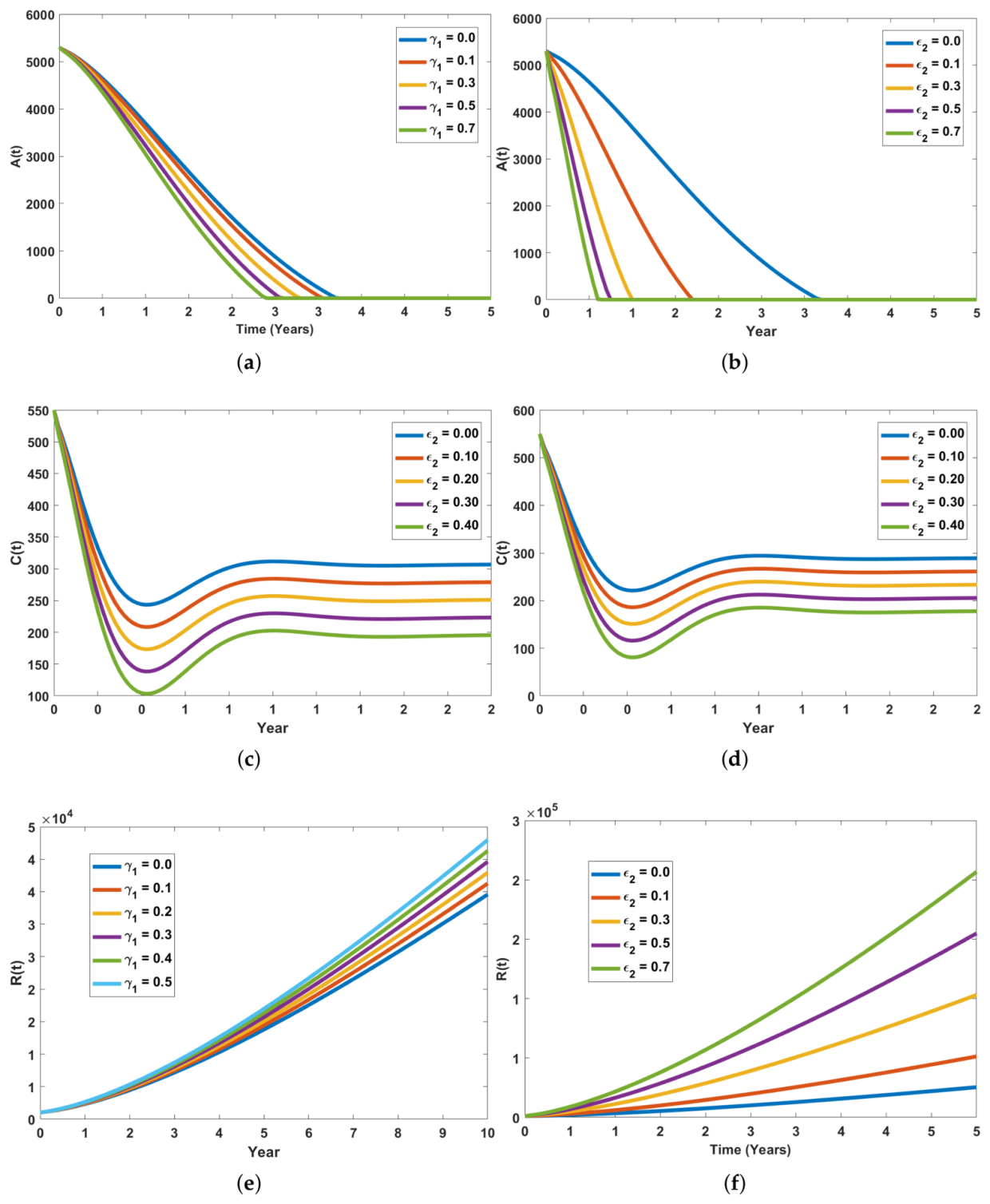
Figure 15.
(a) Impact of treatment on the Chronic compartment. (b) Impact of treatment on the Recovered compartment.
Figure 15.
(a) Impact of treatment on the Chronic compartment. (b) Impact of treatment on the Recovered compartment.
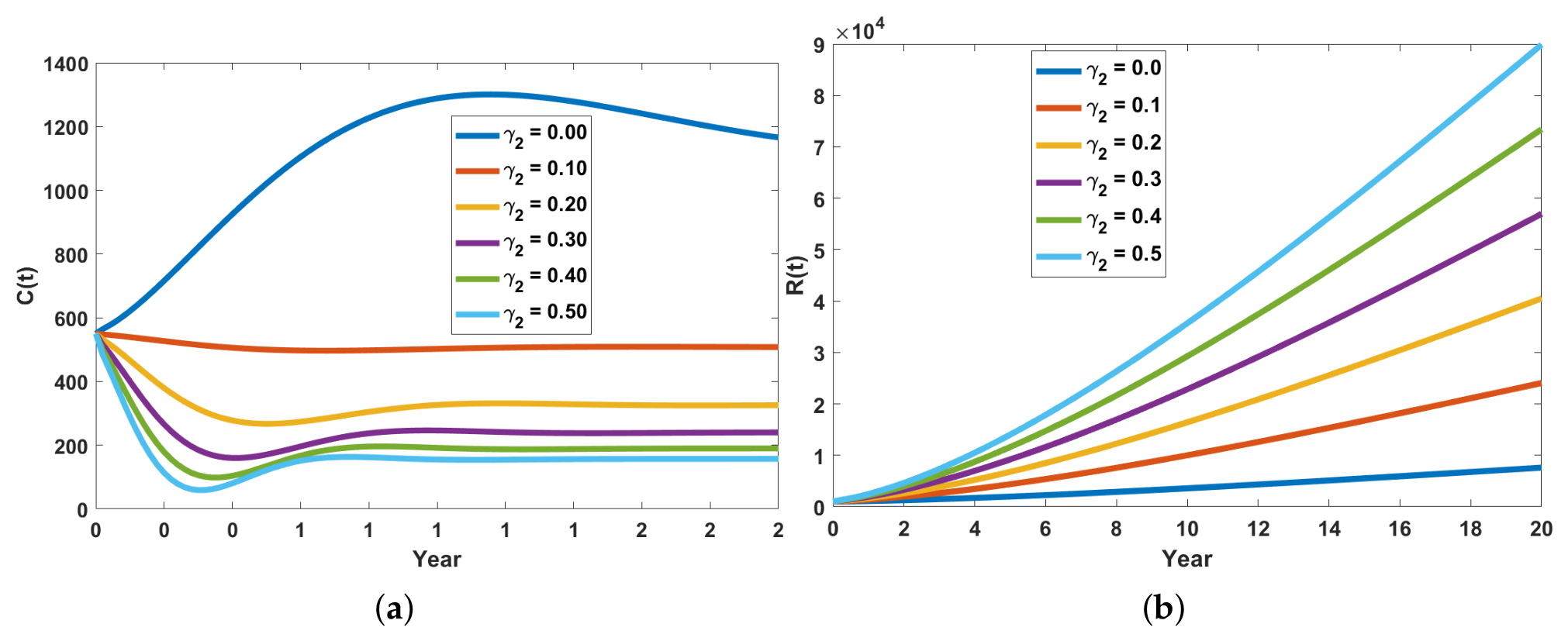

Table 1.
Description of State Variables and Parameters.
| State Variables | Description |
|---|---|
| N | Total population |
| S | Susceptible population |
| V | Vaccinated individuals |
| Q | Screened exposed individuals |
| E | Exposed Individuals in the incubation stage |
| A | Individuals with acute Infection |
| C | Individuals that progressed to chronic stage |
| R | Recovered individuals |
| Parameters | Description |
| Recruitment rate | |
| Contact rate | |
| Screening rate | |
| Effectiveness of screening | |
| PEP rate | |
| Susceptible vaccination rate | |
| Progression rate from exposed to chronic state | |
| Progression rate from exposed to acute state | |
| Progression rate from screened to acute state | |
| Progression rate from acute to chronic state | |
| Rate of managing acute infection | |
| Rate of treating chronic infection | |
| Effectiveness of acute infection management | |
| Chronic Hepatitis B induced death rate | |
| Natural death rate | |
| Rate of compliance to safe practices | |
| Chronic infection modification parameter |
Table 2.
Summary statistics for observed and predicted .
| Statistics | Mean | Std | Mode | Median | Max | Min | RMSE | |
|---|---|---|---|---|---|---|---|---|
| Observed | 39.81 | 26.06 | 14.00 | 32.00 | 95.00 | 10.00 | ||
| Predicted | 37.51 | 21.783 | 16.03 | 30.03 | 81.34 | 16.03 | 0.8258 | 16.21 |
| Difference | 2.30 | 1.97 | -2.03 | 4.28 | -6.03 | 13.66 |
Table 3.
Values of parameters of model.
| Parameter | Values (per year) | CI | Reference |
|---|---|---|---|
| 51450 | Estimated | ||
| [0.00001,0.010] | Fitted | ||
| [0.2959,0.5000] | Fitted | ||
| [22] | |||
| [0.2390,0.5000] | Fitted | ||
| [26] | |||
| Control Parameter | |||
| [0.0001, 0.0036] | Fitted | ||
| [26] | |||
| [0.0074,0.0501] | Fitted | ||
| Control Parameter | |||
| [26] | |||
| [0.1415,0.5000] | Fitted | ||
| [22] | |||
| [0.1340,0.2000] | Fitted | ||
| [0.0044,0.3257] | Fitted | ||
| Estimated |
Table 4.
Forward Normalized Sensitivity Indices.
| Parameter | Elasticity Indices | Values of the Elasticity index |
|---|---|---|
| 1.0000 | ||
| -0.0204 | ||
| 0.5379 | ||
| -0.0004 | ||
| -0.0001 | ||
| -0.0014 | ||
| -0.5248 | ||
| -0.0008 | ||
| 0.1283 | ||
| -0.8658 | ||
| -0.997 | ||
| 0.0001 | ||
| 0.0018 | ||
| 0.6691 | ||
| 0.0001 |
Disclaimer/Publisher’s Note: The statements, opinions and data contained in all publications are solely those of the individual author(s) and contributor(s) and not of MDPI and/or the editor(s). MDPI and/or the editor(s) disclaim responsibility for any injury to people or property resulting from any ideas, methods, instructions or products referred to in the content. |
© 2026 by the authors. Licensee MDPI, Basel, Switzerland. This article is an open access article distributed under the terms and conditions of the Creative Commons Attribution (CC BY) license (http://creativecommons.org/licenses/by/4.0/).
Copyright: This open access article is published under a Creative Commons CC BY 4.0 license, which permit the free download, distribution, and reuse, provided that the author and preprint are cited in any reuse.


