
Submitted:
06 June 2026
Posted:
08 June 2026
You are already at the latest version
Abstract
Nonlinear matrix equation Xp - m∑i=1ATiX-1Ai=Q has extensive applications in control theory, ladder networks, dynamic programming and stochastic filtering. In this paper, we propose a weighted average iterative algorithm to solve this nonlinear matrix equation. Based on the basic characteristics of the Thompson metric space, the convergence and error estimation formula of the algorithm are proved. Numerical experiments to illustrate the feasibility and effectiveness of the proposed algorithm are given.
Keywords:
nonlinear matrix equation
; fixed point iteration algorithm
; Anderson acceleration algorithm
; Thompson metric space
MSC: 15A24, 65F30
1. Introduction
The nonlinear matrix equation
Where p is a positive integer, are non-singular real matrices, and is a positive definite matrix, has been widely used in many fields, such as control theory [1,2], ladder network [3], random filtering [4], statistics [5], etc.
For the nonlinear matrix equation (1.1) with p=1, Duan et al. [6] proved it has a unique positive definite solution and gave the existence interval of the unique Hermitian positive definite solution. They also gave an iterative algorithm to compute the unique Hermitian positive definite solution and a error estimation formula of the iterative approximate solution; Yin et al. [7] considered the perturbation analysis of the positive definite solution, obtained two perturbation bounds of the unique positive definite solution, and derived the expression of the condition number of the unique solution; Li et al. [8] proposed a fixed point accelerated iteration method, and based on the basic characteristics of the Thompson distance, proved the convergence and error estimation of the proposed algorithm. For the general cases of the nonlinear matrix equation (1.1), Lim et al. [9] proved the nonlinear matrix equation with has an unique positive definite solution and gave the existence interval of the unique Hermitian positive definite solution; Jin et al. [10] discussed the solution of the matrix equation through the properties of Thompson metric and two fixed point theorems in ordered Banach spaces, and estimated the bounds of the positive definite solution, and, furthermore, investigated perturbation analysis of the solution with respect to small perturbations on the coefficient matrices. For the similar cases of the nonlinear matrix equation (1.1), Erfanifar et al. [11] first introduced the necessary and sufficient conditions for the existence of the solution of nonlinear matrix equation and then proposed the inversion-free iteration method to find this solution of the nonlinear matrix equation; Liu et al. [12] proposed an iterative algorithm for solving the maximum Hermitian positive definite solution of a nonlinear matrix equation and proved the convergence of proposed algorithm; Li et al. [13,14] derived necessary conditions and sufficient conditions for the existence and uniqueness of the Hermitian positive definite solution for the matrix equation with ; Meng et al. [15] proposed a fixed point iteration method with step parameters to solve the positive definite solution of the matrix equation ; Meng et al. [16] and Mouhadjer et al. [17] studied the nonlinear matrix equation with ; Sayevand et al. [18] studied the nonlinear matrix equation ; Pakhira et al. [19] studied the nonlinear matrix equation with , etc.
In this paper, we propose a weighted average iterative algorithm to solve the nonlinear matrix equation (1.1). Based on the basic characteristics of the Thompson metric space, we will prove the convergence and error estimation formula of the proposed algorithm. Meanwhile, we will give some numerical experiments to illustrate the feasibility and effectiveness of the proposed algorithm.
2. Preliminaries
Let denote the set of real symmetric matrices, denote the set of real symmetric positive semi-definite matrices, and denote the set of real symmetric positive definite matrices. The notations , and represent the conjugate transpose, transpose and Frobenius norm of the matrix , respectively. The notations means , means , and means . The notations and indicate the maximum and minimum eigenvalues of the real symmetric positive definite matrix X, respectively, and indicate the identity matrix of size implied by context.
Definition 2.1.
Thompson distance has the following basic properties:
Lemma 2.1.
hold for any .
Lemma 2.2.
Lemma 2.3.
In addition, the following lemma 2.4 can be obtained by direct calculation according to Thompson’s distance definition:
Lemma 2.4.
For the constant , . We have .
The follow Lemma 2.5 and Lemma 2.6 from [11] can be used to prove the fact that the nonlinear matrix equation (1.1) has a unique positive definite solution in given metric space.
Lemma 2.5.
If is compression mapping on the metric space and has a compression coefficient , then the mapping has a unique fixed point on .
Lemma 2.6.
For any . If , then holds for any , and holds for any .
Lemma 2.7.
Assume that X is a positive definite solution of the nonlinear matrix equation (1.1), then the following inequality holds
Proof.
Since X is a positive definite solution of the nonlinear matrix equation (1.1), then
Hence, we have . And so we have by Lemma 2.6 that
, .
Hence, the inequality (2.1) holds. ■
Let
and
then, we have the following Lemma 2.8.
Lemma 2.8.
The matrix functionsatisfies the Lipschitz condition on Thompson metric space, that is, for any, we have
where
Proof.
It can known from Lemma 2.1, Lemma 2.2, Lemma 2.3 and Lemma 2.6 that
.
Hence, the inequality (2.4) holds. ■
According to Lemma 2.5, Lemma 2.7 and Lemma 2.8, the following lemma can be immediately obtained.
Lemma 2.9.
The nonlinear matrix equation (1.1) has a unique positive definite solution, and, furthermore, its unique positive definite solution X* satisfies given as (2.3).
3. Iterative Algorithm and Its Convergence
This section we first propose a multi-steps weighted average iterative algorithm for solving the nonlinear matrix equation (1.1), and then, based on the basic characteristics of Thompson metric space, prove the convergence of the proposed algorithm and the error estimation formula of the iterative solution. Let . we propose the multi-steps weighted average iterative algorithm to solve the nonlinear matrix equation (1.1) as the following Algorithm 3.1.
Algorithm 3.1 (Weighted average iteration algorithm to solve (1.1)):
Step 1. Given the initial iteration point , error tolerance parametersε, and positive integer s;
Step 2. Calculate , Let ;
Step 3. If , stop (in this case, is an approximate solution of the nonlinear matrix equation (1.1)), otherwise, go to Step 4;
Step 4. Let
Step 5. Calculate ;
Step 6. Let , and if , go to Step 5;
Step 7. Find such that
Step 8. Calculate ;
Step 9. Calculate . Let , and go to Step 3.
For Algorithm 3.1, the following convergence theorem exists.
Theorem 3.1.
The nonlinear matrix equation (1.1) has a unique positive definite solution, and for any initial matrix , the matrix sequence generated by Algorithm 3.1 converges to a unique positive definite solution , and has the following error estimation formula
Proof.
The result that the nonlinear matrix equation (1.1) has a unique positive definite solution X* in Ω given as (2.3}) can be obtained directly by Lemma 2.9, and so we don’t prove it here. We prove the conclusion (2.5) by induction. When k=1and k=2, we have
where , , , . So we have by Lemma 2.2, Lemma 2.4 and Lemma 2.8 that
Assumed that the the conclusion holds for , that is, , then
Hence, by the principle of induction, the error estimation formula holds for all
Notice that the compression coefficient , we have
and this means
Thus, the matrix sequence generated by Algorithm 3.1 converges to the unique positive definite solution of the nonlinear matrix equation (1.1). ■
4. Numerical Experiments
In this section, some numerical experiments will be tested to illustrate the feasibility of Algorithm 3.1. The experiments are divided into two parts. In the first part, the relationship between the fixed points iterations number s and the convergence of the Algorithm 3.1 is analyzed, and the selection range of the best fixed points iterations numbers are given. In the second part, the comparison of the convergence of Algorithm 3.1 with fixed point iterative algorithm [6,20] and Anderson acceleration algorithm [8,21] are given. In all the numerical experiments, the matrices are randomly generated by the MATLAB, that is . To make sure the matrix equation (1.1) has a solution, the matrices Q is chosen as
, .
In all tests, the initial iteration matrix is chosen as , the termination condition is the residual satisfied
. (4.1)
In all data results are obtained in the Window10, 64-bit, Matlab R2013a environment.
4.1. Selection of Fixed Points Iteration Numbers
For each iteration of the Algorithm 3.1, fixed points iteration number (s) has an important relationship with convergence speed. Consider the nonlinear matrix equation
We can be seen from Figure 1 that the convergence speed of Algorithm 3.1 is directly affected by the fixed points iteration number (s) . In general, when s chosen as 5 through 10, Algorithm 3.1 is relatively more efficient than other cases. But how to select the best fixed points iteration number (s) is an important problem which should be studied in future.
4.2. Comparison of Convergence of Different Algorithms
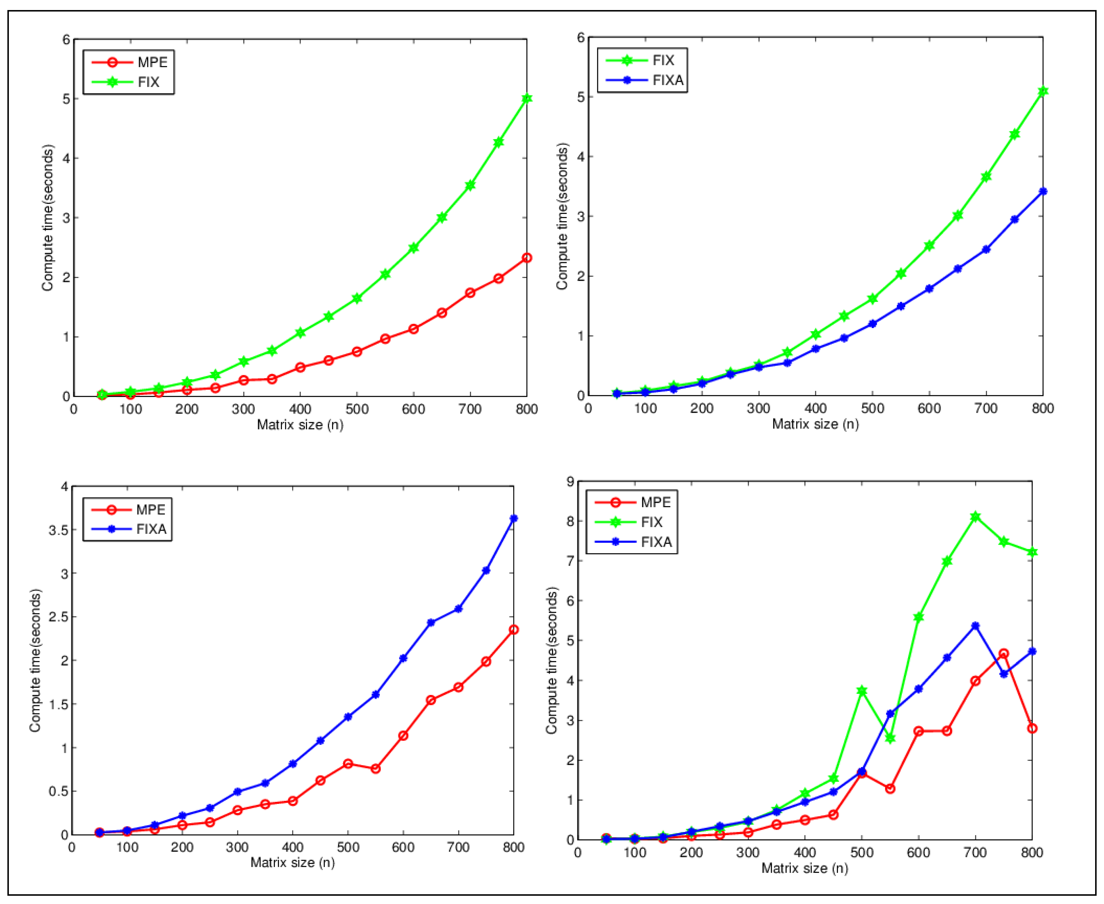
Notice that Algorithm 3.1 is most efficient when the fixed points iteration number s chosen as 5 to 10. Therefore, all the following tests, the fixed points iteration number s in Algorithm 3.1 is fixed at 5. In addition, for the convenience of the expression, we use the notations MPE, FIX and FIXA denote as Algorithm 3.1, fixed-point algorithm proposed in [6,20] and Anderson acceleration algorithm proposed in [8,21], respectively. In all tests, the maximum iteration numbers of each iteration algorithms are restricted to 10000, and the termination condition is the establishment of (4.1). Table 1 and Figure 2 report the comparison of MPE, FIXA and FIX to solve the nonlinear matrix equation (4.2) of the computational time (Time) with different matrix sizes.
Based on the tests reported in Table 1, Figure 2 and many other performed unreported tests which show similar patterns, we have that Algorithm 3.1 is more efficient than the fixed point accelerated iteration algorithm proposed in [8,21] and fixed point algorithm proposed in [6,20].

Table 4.1.
Numerical comparison values of MPE, FIX and FIX with different matrix size.
|
n Time (seconds) Algor |
MPE | FIXA |
FIX |
| 100 | 0.0461 | 0.0285 | 0.0393 |
| 200 | 0.0959 | 0.2193 | 0.1717 |
| 300 | 0.2334 | 0.5372 | 0.4636 |
| 400 | 0.6079 | 1.0863 | 1.2363 |
| 500 | 0.8371 | 1.6197 | 2.1035 |
| 600 | 1.5645 | 2.3805 | 3.2996 |
| 700 | 2.4385 | 3.5413 | 4.8826 |
| 800 | 3.3272 | 4.7722 | 6.8717 |
| 900 | 4.6206 | 6.4310 | 9.6169 |
| 1000 | 6.3372 | 8.2044 | 12.8925 |
| 1100 | 7.7366 | 10.4206 | 16.3306 |
| 1200 | 10.1329 | 12.3955 | 20.7740 |
| 1300 | 16.1424 | 23.8879 | 39.3865 |
| 1400 | 23.5979 | 28.5672 | 48.2884 |
| 1500 | 20.3946 | 20.8011 | 35.7082 |
| 1600 | 22.2414 | 24.5547 | 42.8654 |
| 1700 | 23.6987 | 29.6401 | 48.9275 |
| 1800 | 28.0851 | 34.3586 | 59.1632 |
| 1900 | 32.3917 | 38.3886 | 67.3332 |
| 2000 | 36.9877 | 40.8254 | 76.2251 |
5. Conclusions
In this paper, a weighted average iterative algorithm (Algorithm 3.1) is proposed to solve the nonlinear matrix equation . The convergence and error estimation of the proposed algorithm are proved (Theorem 3.1). Some numerical comparison experiments with existing algorithms are given (Table 1, Figure 2). For Algorithm 3.1, the selection of the fixed point iteration number s is discussed. Problems which should be studied in near future are listed.
Author Contributions
JP wrote the main manuscript text; ST prepared the figures and tables.
Funding
Dr Peng Jingjing, Science and Technology Project of Guangxi (AD25069086) .
Use of AI tools declaration
The authors declare they have not used Artificial Intelligence (AI) tools in the creation of this article. AIMS Mathematics.
Data Availability Statement
The original contributions presented in the study are included in the article; further inquiries can be directed to the corresponding authors.
Conflicts of Interest
The authors declare no conflict of interest.
References
- Abou-Kandil H.; Freiling G.; Ionescu V. Matrix Riccati Equations in Control and Systems Theory, IEEE T. Automat. Contr. 2003, 7, 299-410.
- Gohberg I.; Lancaster P.; Rodman L. Matrix Polynomials, New York: Academic Press,1982.
- Anderson W.N.; Morley T,D.; Trapp G.E. Ladder networks fixpoints and the geometric mean, Circuits, Systems and Signal Processing 1983, 3, 259-268. [CrossRef]
- Pusz W.; Woronowicz S.L. Functional calculus for sesquilinear forms and the purification map, Rep. Math. Phys. 1975, 2, 159-170.
- Bucy R.S. A Priori Bounds for the Riccati Equation, The Regents of the University of California 1972, 3, 645-656.
- Duan X.F.; Cheng H.X.; Duan F.J. Positive defifinite solutions of the matrix equation , Numer. Math. A. J. Chin. Univ. 2012, 34, 141–152.
- Yin X.Y.; Fang L. Perturbation analysis for the positive defifinite solution of the nonlinear matrix equation , J. Appl. Math. Comput. 2013, 43, 199–211.
- Li T.; Peng J.J.; Peng Z.Y.; Tang Z.A.; Zhang Y.S. Fixed-point accelerated iterative method to solve nonlinear matrix equation , Comput. Appl. Math. 2022, 41:415.
- Lim Y. Solving the nonlinear matrix equation via a contraction principle, Linear Algebra Appl. 2009, 4, 1380-1383.
- Jin Z.; Zhai C. Investigation of positive definite solution of nonlinear matrix equation , Comput. Appl. Math. 2021, 40:74.
- Erfanifar R.; Sayevand K.; Hajarian M. An effificient inversion-free method for solving the nonlinear matrix equation , J. Franklin Inst 2022, 359, 3071–3089.
- Liu A.; Chen G. On the Hermitian positive definite solutions of nonlinear matrix equation , Appl. Math. Comput. 2014, 243, 950-959.
- Li J.; Zhang Y.H. The Investigation on two Kinds of Nonlinear Matrix Equations, Bull. Malays. Math. Sci. Soc. 2019, 42, 3323–3341.
- Li J.; Zhang Y.H. Solvability for a Nonlinear Matrix Equation,B. Iran. Math. Soc. 2018, 44, 1171–1184.
- Meng J.; KimH.M. The Positive Definite Solution of the Nonlinear Matrix Equation , Numer. Func. Anal. Opt. 2017, 39, 398-412.
- Meng J.; Chen H.J.; Kim Y.J.; Kim H.M. A further study on a nonlinear matrix equation, Jap. J. Ind. Appl. Math. 2020, 37, 831–849.
- Mouhadjer L.; Benahmed B. A New Inversion-Free Iterative Method for Solving a Class of Nonlinear Matrix Equations, B. Iran. Math. Soc. 2022, 48, 2825–2841. [CrossRef]
- Sayevand K.; Erfanifar R.; Esmaeili H. The maximal positive definite solution of the nonlinear matrix equation ,Math. Sci. 2023,17:4,1-14. https://doi.org/10.1007/s40096-022-00454-4. [CrossRef]
- Pakhira S.; Bose S.; Hossein S.M. Solution of a Class of Nonlinear Matrix Equations, B. Iran. Math. Soc. 2021, 47, 415–434. [CrossRef]
- Ran A.C.; Reurings M.C. A fixed point theorem in partially ordered sets and some applications to matrix equations, Proc. Am. Math. Soc. 2004, 132:5, 1435–1443.
- Walker H.F.; Peng N. Anderson Acceleration for Fixed-Point Iterations, SIAM J. Numer. Anal. 2011, 4, 1715-1735. [CrossRef]
Figure 1.
Fixed points iteration number (s) and compute time curve with different matrix size.
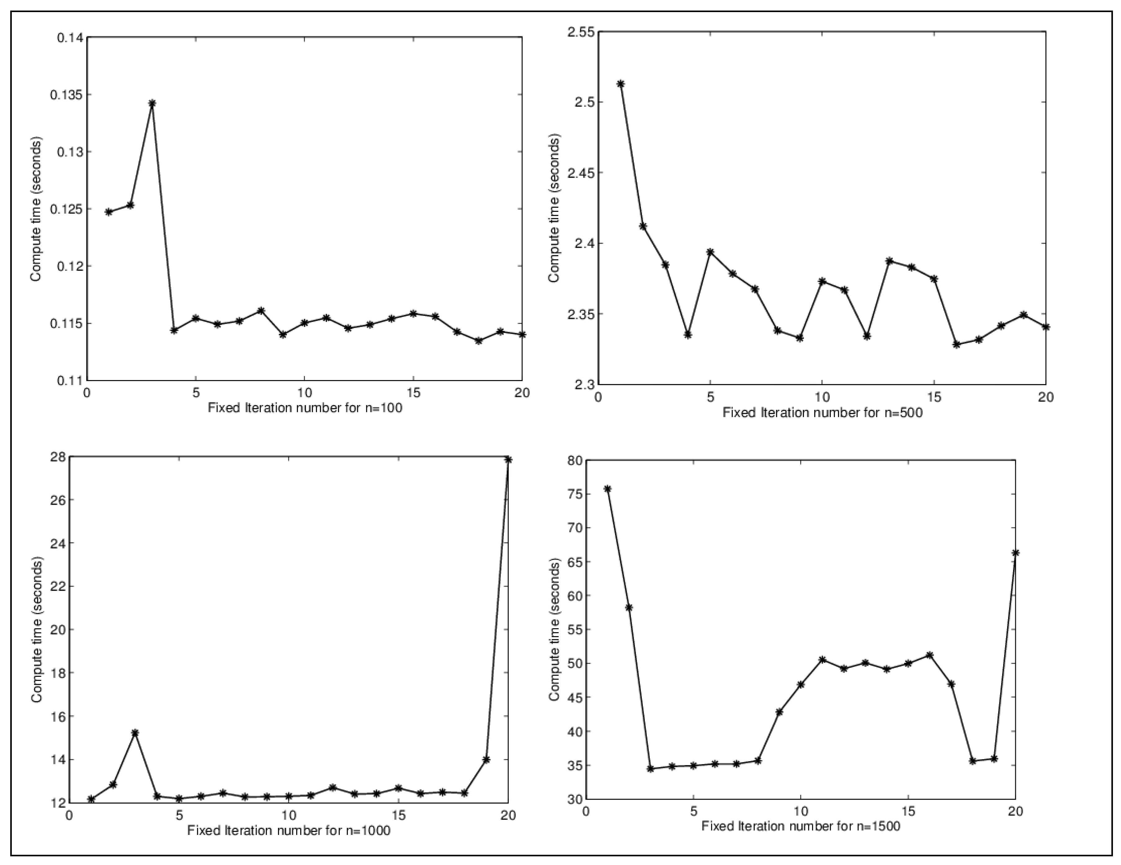
Figure 2.
Numerical comparison curves of FIXA, FIX and MPE with different matrix sizes.
Disclaimer/Publisher’s Note: The statements, opinions and data contained in all publications are solely those of the individual author(s) and contributor(s) and not of MDPI and/or the editor(s). MDPI and/or the editor(s) disclaim responsibility for any injury to people or property resulting from any ideas, methods, instructions or products referred to in the content. |
© 2026 by the authors. Licensee MDPI, Basel, Switzerland. This article is an open access article distributed under the terms and conditions of the Creative Commons Attribution (CC BY) license (http://creativecommons.org/licenses/by/4.0/).
Copyright: This open access article is published under a Creative Commons CC BY 4.0 license, which permit the free download, distribution, and reuse, provided that the author and preprint are cited in any reuse.


