

Submitted:
03 June 2026
Posted:
04 June 2026
You are already at the latest version
Abstract
This study presents a comparative numerical investigation of second-order and fourth-order Runge–Kutta methods for solving chaotic dynamical systems. The Lorenz, Genesio–Tesi, and Rossler systems are considered because of their nonlinear behavior and high sensitivity to initial conditions. The numerical schemes investigated include the Midpoint, Improved Euler, Ralston, and fourth-order Runge–Kutta (RK4) methods. The performance of the methods is evaluated in terms of convergence behavior, numerical accuracy, stability characteristics, and computational cost. Stability analysis of each chaotic system is carried out through equilibrium point determination and Jacobian eigenvalue analysis. Numerical simulations are implemented in MATLAB and comparisons are performed using different step sizes. The results indicate that all numerical methods converge as the step size decreases; however, the RK4 method consistently provides significantly smaller errors and improved stability properties compared with the second-order schemes. The findings further demonstrate that higher-order numerical integration methods provide superior performance for highly sensitive chaotic systems where accuracy and reliability are essential.
Keywords:
Lorenz
; Genesio Tesi
; Rosler
; Runge Kutta methods
; stability
; convergence rate
; computational time
MSC: 65M06; 65M12; 65N06
1. Introduction
The study focuses on investigating the efficiency and effectiveness of solving the Lorenz, Genesio Tesi and Rosler systems of equations by using the Midpoint, Improved Euler’s, Ralson methods and Runge Kutta method of order four. The Lorenz equations is a system of ordinary differential equations which were first studied by a mathematician and meteorologist Edward Lorenz. This system is used to model the unpredictable behavior of weather. They represent the convective motion of fluid cell that is warmed from below and cooled from above [1]. The Genesio-Tesi system is a system of ordinary differential equations which were implemented by Roberto Genesio and Alberto Tesi in 1992 as an electronic circuit. They are made of three-dimensional differential equations with one of them being quadratic. The Rossler system is a system of three nonlinear ordinary differential equations which were studied by Otto Rossler in the 1970s [2]. The ordinary differential equations in the system define a continuous-time dynamical system that exhibits chaotic dynamics associated with fractal properties of the system.
The chaotic system of equations will be solved by using the numerical methods, which are mathematical tools that are designed to solve numerical problems in the study of numerical analysis. In numerical analysis, these numerical methods attempt to find approximate solutions of problems than exact solutions [3]. In theory, a numerical method begins with an initial point and then moves forward in time to find the next solution point. The procedure is repeated in order to map out the solution. To determine the current value, single-step methods refer to only one previous point and its derivative. Runge-Kutta methods, for example, take some intermediate steps to obtain a higher order method, but then discard all previous information before proceeding to the next step, which in contrary to the Multi-step methods which improve efficiency by retaining and using information from previous steps rather than discarding it. In this project the selected numerical methods, the fourth order Runge-Kutta and second order Runge-Kutta methods are used to solve the mathematical problems that are chaotic in nature in order to investigate the accuracy and efficiency of the methods.
The Runge-Kutta methods were developed around the 1990s by two German mathematicians Carl Runge and Wilhelm Kutta [4]. They are a family of implicit and explicit iterative single step methods including the Euler’s method. Runge-Kutta methods are effective and widely used family of numerical methods for solving the initial-value problems of differential equations. The primary disadvantage of these methods is that they require significantly more computational time than multi-step methods whereas their main advantages are that they are easy to implement and stable [5]. We have single step methods such as the Euler, Heun’s, Midpoint and the Ralston methods, which are used to find approximate solutions of Initial Value Problems (IVPs). The main advantage of these other single step methods is that they are simple and direct. They mostly require less evaluations at a point than the Runge-Kutta methods that requires more than just one evaluation at a point to obtain a solution. These methods require less computational time than the Runge-Kutta methods. Although this is the case, the Runge-Kutta methods are more stable than these other single step methods. For instance, the Euler’s methods are conditionally stable. They are only stable when the step size is significantly small [7].
The theory of chaos dates back to 1963 when it was first reported by Lorenz for a system of ordinary differential equations modeling weather phenomena [11]. Since then, a large number of chaotic phenomena and chaotic behavior have been observed and reported in a wide range of systems, including electrical circuits, lasers, fluid dynamics, mechanical devices, population growth, and many other scientific applications [12]. The chaos theory is a study of random or unpredictable behavior in systems [13]. Such behaviour is mostly studied in natural systems such as the weather, biological and physical processes, and electromagnetic processes. Chaos theory states that a system is chaotic if ordered regular patterns can be seen to arise out of random, under certain conditions [14].
The selected chaotic systems are considered to be highly sensitive to their initial conditions, that is, a small change in their initial conditions results in a significant change in the solution. This motivates the investigation and applicability of the fourth order Runge-Kutta and three step Adams Moulton numerical methods. These study presents a novel comparisons of solutions obtained by the Midpoints, improved Eulers, Ralston and Runge Kutta method of order four when solving the Lorenz, Genessio Tesi and Rosler systems of chaotic equations.
The existing literature contains numerous studies on numerical approximations of chaotic systems using Runge–Kutta methods. However, limited studies provide a systematic comparison of multiple second-order Runge–Kutta variants against the fourth-order Runge–Kutta method across different chaotic systems while simultaneously assessing convergence properties, stability characteristics, and computational efficiency. This study addresses this gap through a unified comparative framework using the Lorenz, Genesio–Tesi, and Rössler systems.
2. Problem Formulation
The problems of interest in this research are the Lorenz, Genezio Tesi, and the Rossler chaotic systems. In this chapter, the stability analysis of these systems is done using the Lyapunov stability analysis in the first approximation [23]. The second and fourth orders Runge Kutta methods are derived and applied to the problems.
3. Theoretical Results
3.1. Theorem 1: Existence and Uniqueness of Solution
Theorem
Consider the initial value problem
where is continuous in a region
and satisfies a Lipschitz condition in (y), that is,
for some positive constant .
Then there exists a unique solution of the initial value problem in some interval containing .
Proof
The proof follows directly from the Picard–Lindelöf theorem. Since is continuous and satisfies the Lipschitz condition, successive approximations generated through Picard iteration converge uniformly to a unique solution.
3.2. Theorem 2: Consistency of the Runge–Kutta Methods
Theorem
The Midpoint, Improved Euler, Ralston, and RK4 methods are consistent numerical methods.
Proof
A numerical method is consistent if its local truncation error satisfies
For RK2 methods,
while for RK4,
Thus,
showing that the methods are consistent.
3.3. Theorem 3: Order of Accuracy of RK2 and RK4
Theorem
The Midpoint, Improved Euler, and Ralston methods possess second-order accuracy, while RK4 possesses fourth-order accuracy.
Proof
Expanding the exact solution using Taylor series gives
Comparing the Taylor expansion with the RK2 approximations shows agreement through terms of order , producing local truncation error
and global error
Similarly, RK4 matches terms up to , resulting in
local truncation error and
global error.
Hence the RK2 methods are second-order accurate and RK4 is fourth-order accurate.
3.4. Theorem 4: Convergence of the Runge–Kutta Methods
Theorem
If a numerical method is both consistent and stable, then it is convergent.
Proof
By the Lax Equivalence principle,
Since the considered Runge–Kutta methods are consistent and stable for sufficiently small step sizes, they are convergent.
3.5. Theorem 5: Global Error Bound
Theorem
Assume that (f(t,y)) satisfies the Lipschitz condition with constant (L). Then the global error satisfies
where denotes the local truncation error.
Proof
Using Gronwall’s inequality together with the local truncation error estimate gives the stated bound.
4. Chaotic Systems and Stability Analysis
4.1. Lorenz System
Edward Lorenz derived the system [24], given by the following system of ordinary differential equations
where , , and are greater than zero. These equations (1) were derived by Lorenz to model two-dimensional fluid cell between two parallel plates at different temperatures [25]. In this project we study the case where , , and with initial conditions , , and , which is the case study that Lorenz conducted [26].
4.1.1. Stability Analysis of the Lorenz System
Given the Lorenz system (1), we set , , and to determine the equilibrium points of the system [27]. In setting the Lorenz system equations to zero, we obtain the following equations
Solving equation (84), (85), and (4) simultaneously, we learn that
By substituting and as determined in equation (7) into equation (4), we obtain the following
From equation (7) and (8) we learn that the origin is one the the equilibrium points of the system, that is
It follows from equation (10) that when , and from equation (5), . From this we learn that the Lorenz system has two more equilibrium points which are
and
By substituting the parameters , , and , the equilibrium points of the system are
To analyse the stability of the system, a Jacobian matrix [27] of the form is constructed. Where
such that
is the Jacobian matrix corresponding to the system.
By finding the first partial derivatives of equation (14), (15), and (16) with respect to u, v and s, and substituting them into the Jacobian matrix (17) we obtain the following Jacobian matrix
Using the given parameters of , and for the Lorenz system (1) the Jacobian matrix becomes
To make conclusions about the stability of the system, the eigenvalues of the Jacobian matrix (19) are determined with respect to each equilibrium point [27], that is
For the equilibrium point
is greater than zero, this implies that the equilibrium point is unstable.
Subsequently, the same procedure is followed to determine the eigenvalues for the other equilibrium points and .
The real parts of and are all greater than zero, this suggests that is an unstable equilibrium point.
The real parts of and are all greater than zero, this suggests that is an unstable equilibrium point.
For the given values of the parameters of , and , none of the equilibrium points of the Lorenz system are stable. This implies that the system is unstable at all its equilibrium points.
4.2. Genesio-Tesi System
This system was proposed by Roberto Genesio and Alberto Tesi [28]. It is given by the following differential equations
where the parameters , , and with initial conditions , and . It is said that the three ordinary differential equations of this system depend on real negative parameters of , , and [29].
4.2.1. Stability Analysis of the Genesio Tesi System
Given the Genesio Tesi System (33), we set , , and to determine the equilibrium points of the system. This leads to the following the equations
We learn from equation (34) and (35) that v=0 and s=0, using this in equation (36) we obtain
For the stated parameters of , , and of the system (33), we learn that the equilibrium point (39) is
By setting
and finding the first partial derivatives with respect to u, v, s of equation (41), (42) and (43) to construct a Jacobian matrix (17) corresponding to the system , we obtain
The eigenvalues of the Jacobian matrix (45) with respect to the equilibrium point (38) are given by
which leads to the following equation.
The real parts of and are both greater than zero, this means that the equilibrium point (38) is unstable.
The eigenvalues corresponding to the Jacobian matrix (45) with respect to the equilibrium point (40) are given by
Determining the eigenvalues from equation (50) we obtain
We learn that is greater than zero, this implies that the equilibrium point of the system is also unstable.
The Genesio Tesi system (33) is unstable at both of its equilibrium points. This means that for the stated parameters of , and , the system is unstable.
4.3. Rossler System
The system was studied by Otto Rossler [2]. It is represented by the following set of ordinary differential equations
where the parameters , , and are greater than zero. The system (55) defines a continuous-time dynamical system that exhibits chaotic dynamics with the fractal properties of the attractor for selected values of , and [17]. Rossler observed a chaotic behavior when conducting the study [30] with , , and subject to the initial conditions , , and .
4.3.1. Stability Analysis of the Rossler System
Given the Rossler system (55), by setting , , and to find the equilibrium points of the system, we obtain the following equations
By substituting from equation (59) into equation (57) we obtain
From equation (60) , using this in equation (58), it follows that
For the stated parameters of , , and of the system (55), the equilibrium points (64) and (65) of the system are
By letting
and finding the first partial derivatives of (68), (69) and (70) with respect to u, v, s to construct a Jacobian matrix (17) corresponding to the system we obtain
The eigenvalues of the Jacobian matrix with respect to the equilibrium point (66) are determined by evaluating
Evaluating equation (72) gives
The real parts of and are greater than zero, this indicates that the equilibrium point is unstable.
The eigenvalues of the Jacobian matrix (71) with respect to the equilibrium point (67). are determined by evaluating
Evaluating (77) gives
The real parts of and are greater than zero, this indicates that the equilibrium point is also unstable.
The Rossler system (55) is unstable at all its equilibrium points for the stated parameters of , , and .
4.4. Derivation of the Runge-Kutta Methods of Order Two and Four
The second order Runge-Kutta method forms part of the family of explicit iterative Runge-Kutta methods. It is used to solve ordinary differential equations of the form given an initial condition . It provides the approximate value of y for a given point x. It is considered to be more effective than the other explicit Runge-Kutta methods as its local truncation error is of order 5 (i.e., ) [31].
The general s-stage Runge–Kutta recurrence formula is
where the stage values are defined by
The coefficients ,, and define the specific Runge-Kutta method.
with
The Taylor series expansion of about is given as follows
where
By substituting equation 85 into 84 with the use of Taylor expansion, we obtain the following equation
Since we have 3 equations and 4 unknowns, we can assume the value of one of the unknowns. The other three will then be determined from the three equations. Generally the value of is chosen to evaluate the other three constants. The three values generally used for are , 1 and , and are known as Heun’s Method, the midpoint method and Ralston’s method, respectively. The Improved Euler’s(Heun’s method) is given as follow:
where
The Midpoint is given as follow:
where
The Ralston’s method is given as follow:
where
4.5. Derivation of Runge-Kutta Method of Order Four
The fourth order Runge-Kutta method forms part of the family of explicit iterative Runge-Kutta methods. It is used to solve ordinary differential equations of the form given an initial condition . It provides the approximate value of y for a given point x. It is considered to be more effective than the other explicit Runge-Kutta methods as its local truncation error is of order 5 (i.e., ) [31].
In general, the Runge-Kutta method of order is given by
where
where the fixed scalars , and are the coefficients of the Runge Kutta formula.
In order to derive the 4th order Runge-Kutta method, we obtain the following recurrence equation for the 4th order Runge-Kutta method from (100)
where,
Therefore, by using the Taylor method to expand the terms (104) of the Runge Kutta method (102) we obtain the following
By substituting (105) into equation (102) gives the following equation
Using the Taylor method to expand equation (106) on the right gives
Comparing the coefficients of equation (107) and equation (106) we obtain the following system of equations
Solving the above system of equation gives , , , and . It then follows that equation (102), which is the Runge Kutta method of order 4 is
5. Algorithm Addition
Algorithm 1: Numerical Solution Procedure
- 1.
- Define chaotic system parameters
- 2.
- Specify initial conditions
- 3.
- Select step size h
- 4.
- Implement Midpoint method
- 5.
- Implement Improved Euler method
- 6.
- Implement Ralston method
- 7.
- Implement RK4 method
- 8.
- Compute numerical solutions
- 9.
- Determine infinity norm errors
- 10.
- Evaluate convergence rates
- 11.
- Compute computational time
- 12.
- Compare numerical results
- 13.
- Plot trajectories and phase portraits
6. Results and Discussion
MATLAB implementation details of Runge–Kutta methods.
For the Lorenz system in Table 1, all second-order methods (Midpoint, Improved Euler, and Ralston) exhibit relatively large errors for coarse step sizes. As the step size decreases from to , the errors reduce significantly, confirming convergence of the methods. Among the second-order schemes, the Improved Euler method initially produces slightly smaller errors than the Midpoint and Ralston methods, while the Ralston method shows competitive performance for smaller step sizes. However, the RK4 method clearly outperforms all second-order methods, producing errors several orders of magnitude smaller across all step sizes. For example, at h=0.00500, RK4 attains an error of , whereas the second-order methods still produce errors of order to . This behaviour confirms the superior accuracy and stability of the fourth-order Runge–Kutta scheme for highly sensitive chaotic systems such as the Lorenz equations. Table 2 presents the convergence results for the Genesio system. The Midpoint, Improved Euler, and Ralston methods display nearly identical error values for all step sizes, indicating that these second-order methods possess comparable numerical behaviour for this problem. The errors decrease consistently as the step size is refined, which verifies the expected convergence property of the methods. The RK4 method again provides substantially smaller errors than the second-order methods. Interestingly, the RK4 error remains almost constant around even as the step size decreases. This suggests that the method has already reached a very high level of accuracy, where further refinement of the step size contributes only marginal improvement, possibly due to machine precision limitations or accumulated round-off effects.
Similarly, the results for the Rossler system in Table 3 indicate strong convergence properties for all methods. The Midpoint, Improved Euler, and Ralston methods again produce identical numerical errors, with the error decreasing rapidly when the step size is reduced from to . However, beyond this point, the reduction becomes less pronounced, indicating that the solutions are approaching a limiting numerical accuracy. The RK4 method consistently achieves the smallest errors, approximately , and remains highly stable for all step sizes considered. The near-constant RK4 error for smaller step sizes further demonstrates the robustness and efficiency of the fourth-order method for solving chaotic dynamical systems.
The numerical results presented in Table 1, Table 2 and Table 3 illustrate the convergence behaviour of the Midpoint, Improved Euler, Ralston, and RK4 methods when applied to the Lorenz, Genesio, and Rossler chaotic systems. In general, the results demonstrate that decreasing the step size h improves the numerical accuracy of all methods, although the rate of improvement differs among the schemes and dynamical systems considered. The numerical experiments confirm that all methods converge as the step size decreases, but the RK4 method provides the highest accuracy and best stability characteristics among the methods investigated. The second-order methods are computationally simpler and still produce acceptable approximations for sufficiently small step sizes, but their errors remain significantly larger than those of RK4, particularly for strongly nonlinear and chaotic systems such as the Lorenz model. These findings demonstrate the advantage of higher-order numerical integration techniques when solving sensitive dynamical systems where accuracy is critical.
The results presented in Table 4 illustrate that the computational results show that the performance of the numerical methods varies depending on the chaotic system being solved. RK4 achieved the best computational efficiency for the Lorenz system, while the Ralston method performed best for the Genesio–Tesi system, and the Midpoint method was most efficient for the Rössler system. Although RK4 is a higher-order method, it did not consistently produce the lowest computational cost across all systems. Overall, the findings indicate that computational efficiency is problem dependent, and lower-order methods can sometimes outperform higher-order methods for certain chaotic systems.
The infinity norm plots shown in Figure 1, Figure 2 and Figure 3 further validate the theoretical orders of convergence of the methods. The slopes corresponding to the second-order methods align closely with , while the RK4 method follows the expected convergence trend. This agreement between theoretical and numerical convergence confirms the correctness of the implementation of the methods.
The time evolution plots and phase portraits presented in Figure 1, Figure 2, Figure 3, Figure 4, Figure 5, Figure 6, Figure 7, Figure 8, Figure 9, Figure 10, Figure 11, Figure 12, Figure 13, Figure 14, Figure 15, Figure 16, Figure 17, Figure 18 and Figure 19 illustrate the qualitative behaviour of the chaotic systems. The numerical solutions generated by all methods generally followed similar trajectories, especially for smaller step sizes. However, the RK4 solutions remained smoother and more stable over longer integration intervals, whereas slight deviations became visible in the second-order methods due to accumulated truncation errors. The phase portraits also successfully captured the chaotic attractors associated with the Lorenz, Genesio–Tesi, and Rossler systems, demonstrating that the numerical schemes were capable of reproducing the essential dynamics of the systems.
The results indicate that while the Midpoint, Improved Euler, and Ralston methods are computationally simpler and easier to implement, they are less accurate for highly sensitive chaotic systems. In contrast, the RK4 method provides significantly better numerical accuracy, stronger stability properties, and more reliable long-term approximations. These findings highlight the importance of using higher-order numerical integration techniques when solving nonlinear chaotic differential equations where precision and stability are critical.
The superior performance of RK4 can be attributed to its higher-order truncation accuracy and multiple intermediate evaluations within each time step. Chaotic systems are highly sensitive to small perturbations, and numerical errors propagate rapidly over time. The RK4 method effectively reduces the accumulation of these local errors, thereby providing more stable long-term approximations than second-order methods.
Future work may extend this analysis to adaptive Runge–Kutta methods, fractional chaotic systems, and hybrid machine-learning-assisted numerical solvers.
7. Conclusions
This study investigated the efficiency and effectiveness of the Midpoint, Improved Euler, Ralston, and fourth-order Runge Kutta numerical methods when solving the Lorenz, Genesio Tesi, and Rossler chaotic systems. The stability analysis showed that all selected systems are unstable at their equilibrium points, confirming their chaotic nature and sensitivity to initial conditions.
The numerical experiments demonstrated that all methods converge as the step size decreases. However, the RK4 method consistently produced the smallest errors and exhibited superior stability and convergence properties compared to the second-order methods. The Midpoint, Improved Euler, and Ralston methods produced acceptable approximations for sufficiently small step sizes, but their errors remained considerably larger than those of RK4, especially for the Lorenz system where chaotic effects are more pronounced.
The infinity norm analysis and graphical comparisons confirmed the theoretical convergence orders of the methods, with the second-order schemes following convergence and RK4 following . Furthermore, the phase portraits and solution trajectories successfully reproduced the chaotic dynamics of the systems under consideration.
Based on the obtained results, it can be concluded that the fourth order Runge Kutta method is the most efficient and reliable method among the investigated schemes for solving chaotic systems of ordinary differential equations. Its high accuracy, improved stability, and robustness make it highly suitable for nonlinear and highly sensitive dynamical systems. Future studies may extend this work by investigating adaptive step-size Runge Kutta methods, implicit schemes, or machine learning-based numerical approaches for solving more complex chaotic and hyperchaotic systems.
Author Contributions
Formal analysis, N.N.; Investigation, N.N.; Supervision, N.N.; Writing—original draft, N.N.; Writing—review editing, N.N. I have read and agreed to the published version of the manuscript.
Funding
This work is funded by the University of Venda. The authors wish to acknowledge the financial support from University of Venda.
Data Availability Statement
The original contributions presented in this study are included in the article. Further inquiries can be directed to the corresponding author.
Acknowledgments
The authors wish to acknowledge the financial support from University of Venda.
Conflicts of Interest
The authors declare that there is no conflict of interests regarding the publication of this paper.
Abbreviations
| Abbreviations: | |
| ADR | Advection–Diffusion–Reaction Equation |
| PINNs | Physics-Informed Neural Networks |
| NSFD | Non-Standard Finite Difference |
| CPU time | Computational time |
| Nomenclature: | |
| x | Spatial variable |
| t | time variable |
| Change in spatial variable | |
| Change in time variable |
References
- Buscarino, A.; Fortuna, L.; Frasca, M.; Sciuto, G. A concise guide to chaotic electronic circuits; Springer International Publishing: Heidelberg, Germany, 2014. [Google Scholar]
- Letellier, C.; Roulin, E.; Rössler, O.E. Inequivalent topologies of chaos in simple equations. Chaos Solitons Fractals 2006, 28(2), 337–360. [Google Scholar] [CrossRef]
- Suli, E.; Mayers, D.F. and University of Oxford. Solution of Equations by iteration. An Introduction to Numerical Analysis. 2003; pp. 2–35. [Google Scholar]
- Butcher, J.C. A history of Runge-Kutta methods. Appl. Numer. Math. 1996, 20(3), 247–260. [Google Scholar] [CrossRef]
- Ahamad, N.; Charan, S. Study of numerical solution of fourth order ordinary differential equations by fifth order runge-kutta method. Int. J. Sci. Res. Sci. Eng. Technol. 2019, 6(1), 230–238. [Google Scholar] [CrossRef]
- Hahn, G.D. A modified Euler method for dynamic analyses. Int. J. Numer. Methods Eng. 1991, 32(5), 943–955. [Google Scholar] [CrossRef]
- Hahn, G.D. A modified Euler method for dynamic analyses. Int. J. Numer. Methods Eng. 1991, 32(5), 943–955. [Google Scholar] [CrossRef]
- Bashforth, F.; Adams, J.C. An attempt to test the theories of capillary action by comparing the theoretical and measured forms of drops of fluid; University Press, 1883. [Google Scholar]
- Dattani, N.S. Linear multistep numerical methods for ordinary differential equations. arXiv 2008, arXiv:0810.4965. [Google Scholar] [CrossRef]
- Reibman, A.; Trivedi, K. Numerical transient analysis of Markov models. Comput. Oper. Res. 1988, 15(1), 19–36. [Google Scholar] [CrossRef]
- Kapitaniak, T. Chaotic oscillations in mechanical systems; Manchester University Press, 1991. [Google Scholar]
- Oestreicher, C. A history of chaos theory. Dialogues in clinical neuroscience. 2022. [Google Scholar]
- Marion, R. Complexity theory for organizations and organizational leadership. Complexity leadership, part, 1. 2008; 1, pp. 1–15. [Google Scholar]
- Mann, S.R. Chaos theory and strategic thought; Army War Coll Carlisle Barracks PA, 1992. [Google Scholar]
- Lorenz, E.N.; Haman, K. The essence of chaos. Pure Appl. Geophys. 1996, 147(3), 598–599. [Google Scholar]
- Gleick, J. Chaos: Making a new science; Penguin, 2008. [Google Scholar]
- Dlamini, P.G. On spectral relaxation and compact finite difference schemes for ordinary and partial differential equations; University of Johannesburg (South Africa), 2015. [Google Scholar]
- Dogan, N. Numerical solution of chaotic Genesio system with multi-step Laplace Adomian decomposition method. Kuwait J. Sci. 2013, 40(1). [Google Scholar]
- Eftekhari, S.A.; Jafari, A.A. Numerical simulation of chaotic dynamical systems by the method of differential quadrature. Sci. Iran. 2012, 19(5), 1299–1315. [Google Scholar] [CrossRef]
- Jun-Mei, L.; Yu-Lan, W.; Zhang, W. Numerical Simulation of the Lorenz-Type Chaotic System Using Barycentric Lagrange Interpolation Collocation Method. Advances in Mathematical Physics. 2019.
- Ghorbani, A.; Saberi-Nadjafi, J. A piecewise-spectral parametric iteration method for solving the nonlinear chaotic Genesio system. Math. Comput. Model. 2011, 54(1-2), 131–139. [Google Scholar] [CrossRef]
- Moaddy, K.; Hashim, I.; Momani, S. Non-standard finite difference schemes for solving fractional-order Rössler chaotic and hyperchaotic systems. Comput. Math. With Appl. 2011, 62(3), 1068–1074. [Google Scholar] [CrossRef]
- Unbehauen, H. (Ed.) Control systems, robotics and automation-volume III: System Analysis and Control: Classical Approaches-III; EOLSS Publications, 2009. [Google Scholar]
- Leonov, G.A.; Kuznetsov, N.V. On differences and similarities in the analysis of Lorenz, Chen, and Lu systems. In Applied Mathematics and Computation; 2015; Volume 256, pp. 334–343. [Google Scholar]
- Mathale, D.; Dlamini, P.G.; Khumalo, M. Compact finite difference relaxation method for chaotic and hyperchaotic initial value systems. 2018, 37(4), 5187–5202. [Google Scholar] [CrossRef]
- Lorenz, E.N. 1996, September. Predictability: A problem partly solved. In Proc. Seminar on predictability (Vol. 1, No. 1). No. 1.
- DeJesus, E.X.; Kaufman, C. Routh-Hurwitz criterion in the examination of eigenvalues of a system of nonlinear ordinary differential equations. Phys. Rev. A 1987, 35(12), 5288. [Google Scholar] [CrossRef]
- Faieghi, M.R.; Delavari, H. Chaos in fractional-order Genesio–Tesi system and its synchronization. Commun. Nonlinear Sci. Numer. Simul. 2012, 17(2), 731–741. [Google Scholar] [CrossRef]
- Wu, X.; Wu, H.; Yan, Z.; Huang, Y. Chaos Anti-Synchronization between Chen System and Genesio System. Open Access Libr. J. 2016, 3(7), 1. [Google Scholar] [CrossRef]
- Li, C.; Hu, W.; Sprott, J.C.; Wang, X. Multistability in symmetric chaotic systems. Eur. Phys. J. Spec. Top. 2015, 224(8), 1493–1506. [Google Scholar] [CrossRef]
- Carpenter, M.H.; Kennedy, C.A. Fourth-order 2N-storage Runge-Kutta schemes (No. NASA-TM-109112). No. NASA-TM-1091121994. [Google Scholar]
- Peinado, J.; Ibáñez, J.; Arias, E.; Hernández, V. Adams–Bashforth and Adams–Moulton methods for solving differential Riccati equations. Comput. Math. With Appl. 2010, 60(11), 3032–3045. [Google Scholar] [CrossRef]
- Kaps, P.; Rentrop, P. Generalized Runge-Kutta methods of order four with stepsize control for stiff ordinary differential equations. Numer. Math. 1979, 33(1), 55–68. [Google Scholar] [CrossRef]
- Amma, B.B.; Melliani, S.; Chadli, L.S. Numerical solution of intuitionistic fuzzy differential equations by Runge-Kutta Method of order four. Notes Intuitionistic Fuzzy Sets 2016, 22(4), 42–52. [Google Scholar]
- Galeone, L.; Garrappa, R. Fractional adams–moulton methods. Math. Comput. Simul. 2008, 79(4), 1358–1367. [Google Scholar] [CrossRef]
- Park, J.H. Synchronization of Genesio chaotic system via backstepping approach. Chaos Solitons Fractals 2006, 27(5), 1369–1375. [Google Scholar] [CrossRef]
- Ogata, S.; Iwayama, T.; Terachi, S. Effect of system noise on chaotic behavior in Roessler type nonlinear system. Int. J. Bifurc. Chaos 1997, 7(12), 2871–2879. [Google Scholar] [CrossRef]
- Yu, Y.; Li, H.X.; Wang, S.; Yu, J. Dynamic analysis of a fractional-order Lorenz chaotic system. Chaos Solitons Fractals 2009, 42(2), 1181–1189. [Google Scholar] [CrossRef]
- Roman, P. Application of the Adams-Bashfort-Mowlton method to the numerical study of linear fractional oscillators models. AIP Conf. Proc. 2021, Vol. 2365(No. 1), 020007. [Google Scholar]
Figure 1.
Comparison Infinity norm error when solving the Lorenz System by Midpoint, Improved Eulers, Ralston and RK4 Methods.
Figure 1.
Comparison Infinity norm error when solving the Lorenz System by Midpoint, Improved Eulers, Ralston and RK4 Methods.
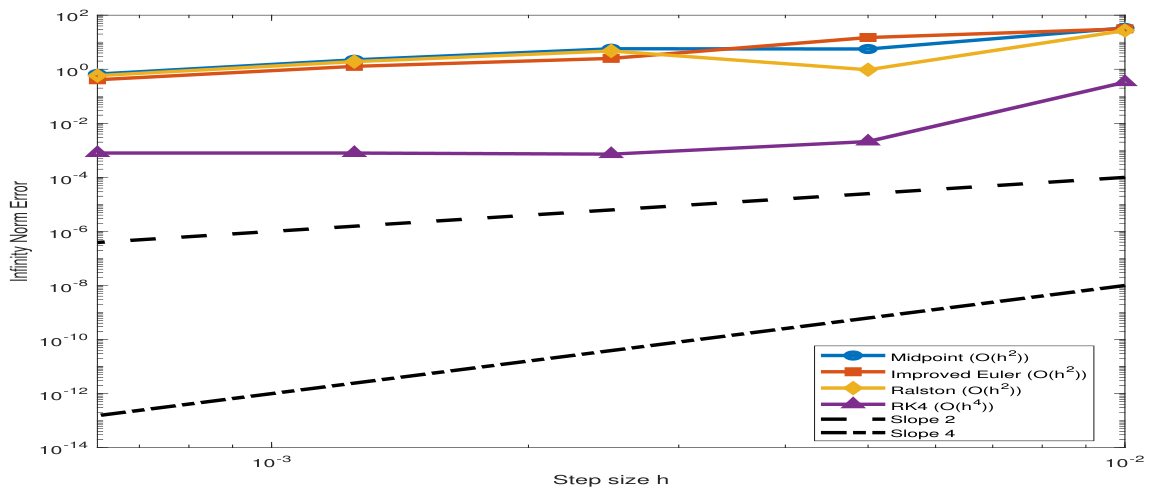
Figure 2.
Comparison Infinity norm error when solving the Genesio Tesi System by Midpoint, Improved Eulers, Ralston and RK4 Methods.
Figure 2.
Comparison Infinity norm error when solving the Genesio Tesi System by Midpoint, Improved Eulers, Ralston and RK4 Methods.
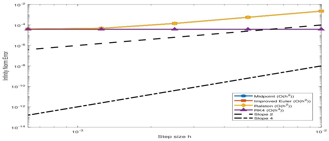
Figure 3.
Comparison Infinity norm error when solving the Rossler System by Midpoint, Improved Eulers, Ralston and RK4 Methods.
Figure 3.
Comparison Infinity norm error when solving the Rossler System by Midpoint, Improved Eulers, Ralston and RK4 Methods.
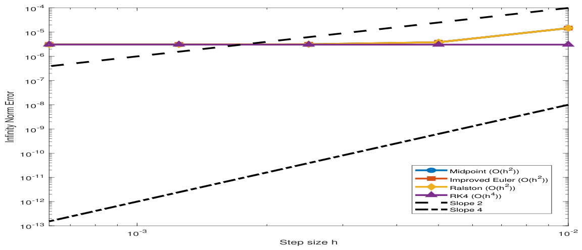
Figure 4.
Comparison of solution u when solving the Lorenz System by the Midpoint, Improved Eulers, Ralston and RK4 Methods with .
Figure 4.
Comparison of solution u when solving the Lorenz System by the Midpoint, Improved Eulers, Ralston and RK4 Methods with .
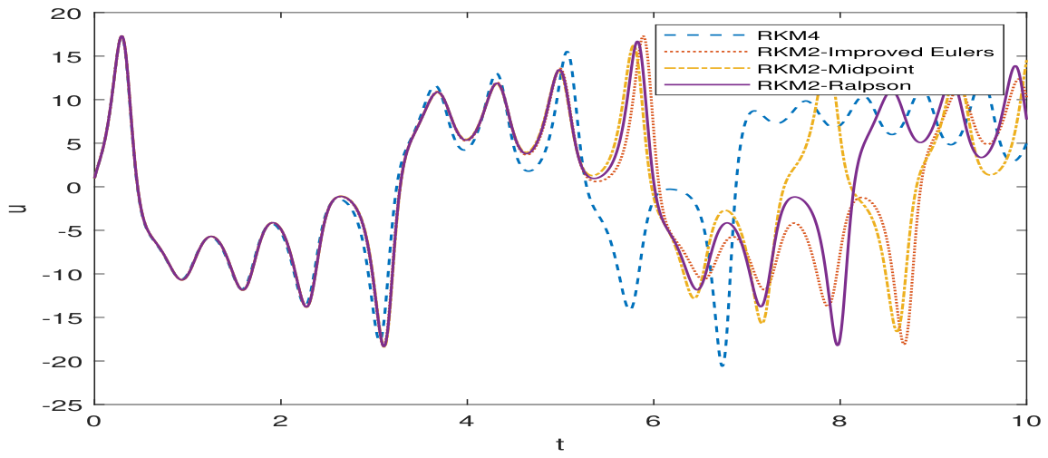
Figure 5.
Comparison of solution v when solving the Lorenz System by the Midpoint, Improved Eulers, Ralston and RK4 Methods with .
Figure 5.
Comparison of solution v when solving the Lorenz System by the Midpoint, Improved Eulers, Ralston and RK4 Methods with .
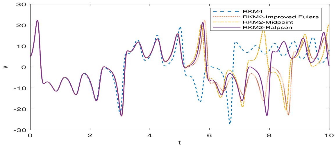
Figure 6.
Comparison of solution s when solving the Lorenz System by the Midpoint, Improved Eulers, Ralston and RK4 Methods with .
Figure 6.
Comparison of solution s when solving the Lorenz System by the Midpoint, Improved Eulers, Ralston and RK4 Methods with .
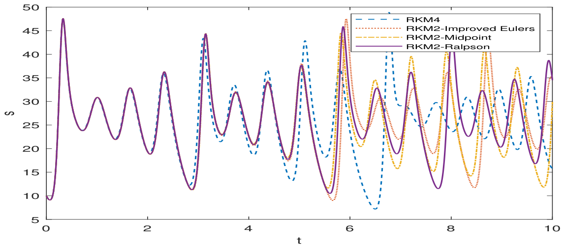
Figure 7.
Solution u versus v when solving the Lorenz System with .
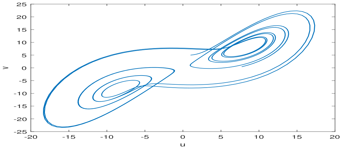
Figure 8.
Solution u versus s when solving the Lorenz System with .
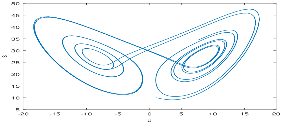
Figure 9.
Solution v versus s when solving the Lorenz System with .
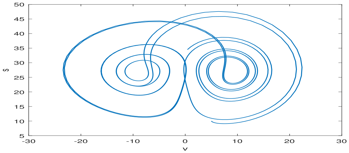
Figure 10.
Comparison of solution u when solving the Genesio System by the Midpoint, Improved Eulers, Ralston and RK4 Methods with .
Figure 10.
Comparison of solution u when solving the Genesio System by the Midpoint, Improved Eulers, Ralston and RK4 Methods with .
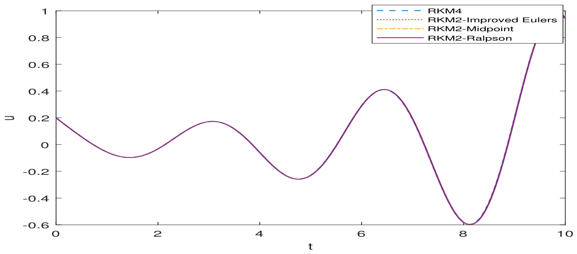
Figure 11.
Comparison of solution v when solving the Genesio System by the Midpoint, Improved Eulers, Ralston and RK4 Methods with .
Figure 11.
Comparison of solution v when solving the Genesio System by the Midpoint, Improved Eulers, Ralston and RK4 Methods with .
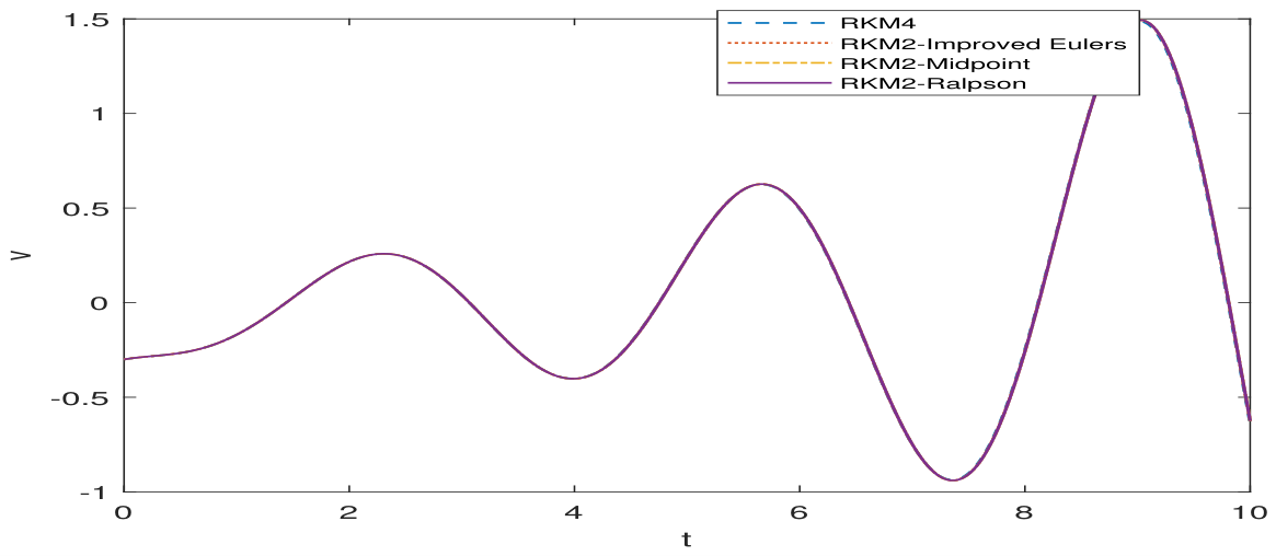
Figure 12.
Comparison of solution s when solving the Genesio System by the Midpoint, Improved Eulers, Ralston and RK4 Methods with .
Figure 12.
Comparison of solution s when solving the Genesio System by the Midpoint, Improved Eulers, Ralston and RK4 Methods with .
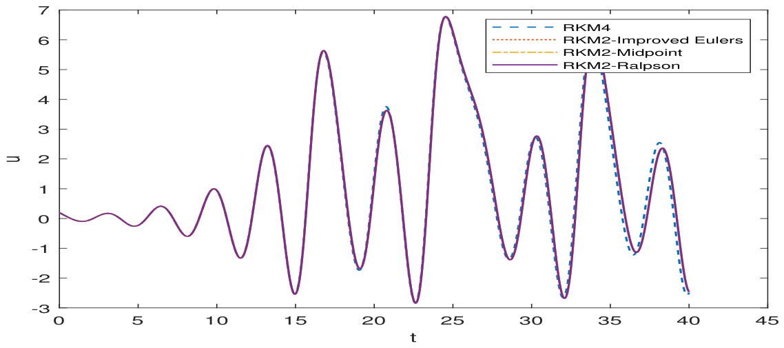
Figure 13.
Solution u versus v when solving the Genesio System with .
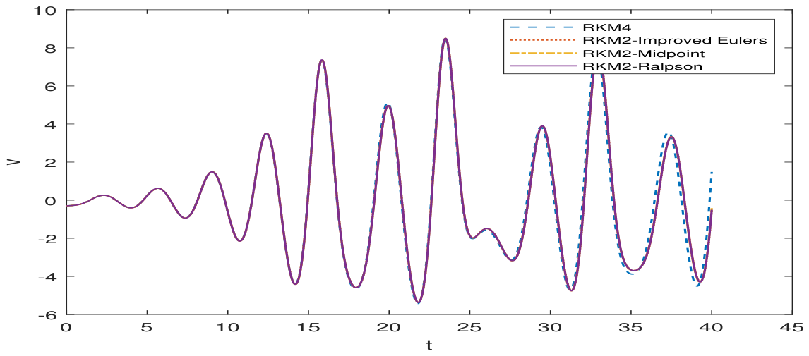
Figure 14.
Solution u and v versus s when solving the Genesio System with .
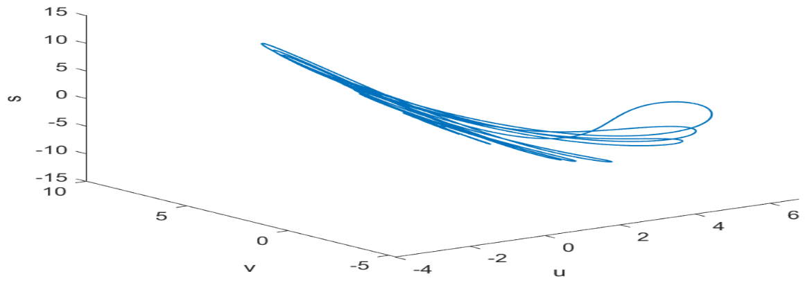
Figure 15.
Comparison of solution u when solving the Rosler System by the Midpoint, Improved Eulers, Ralston and RK4 Methods with .
Figure 15.
Comparison of solution u when solving the Rosler System by the Midpoint, Improved Eulers, Ralston and RK4 Methods with .
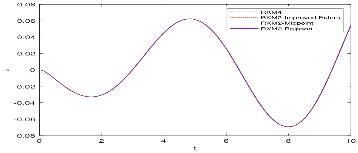
Figure 16.
Comparison of solution v when solving the Rosler System by the Midpoint, Improved Eulers, Ralston and RK4 Methods with .
Figure 16.
Comparison of solution v when solving the Rosler System by the Midpoint, Improved Eulers, Ralston and RK4 Methods with .
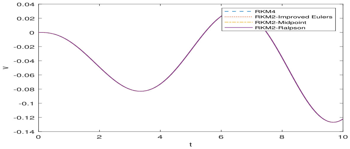
Figure 17.
Comparison of solution s when solving the Genesio System by the Midpoint, Improved Eulers, Ralston and RK4 Methods with .
Figure 17.
Comparison of solution s when solving the Genesio System by the Midpoint, Improved Eulers, Ralston and RK4 Methods with .
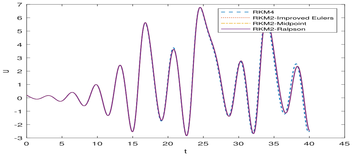
Figure 18.
Solution u versus v when solving the Rosler System with .
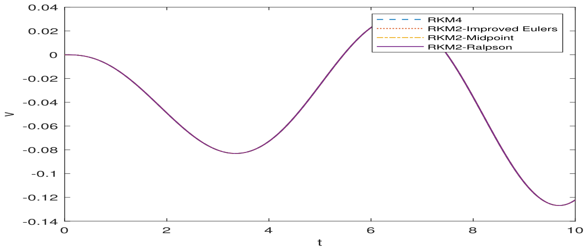
Figure 19.
Solution u and v versus s when solving the Rosler System with .
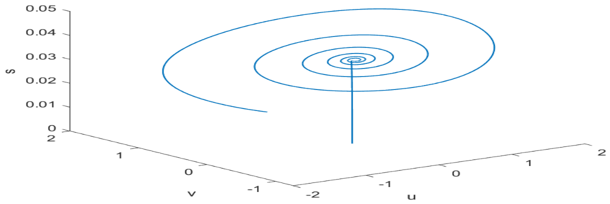

Table 1.
Convergence Rate for the Lorenz System
| h | Midpoint | Improved Euler | Ralston | RKM4 |
|---|---|---|---|---|
| 0.01000 | ||||
| 0.00500 | ||||
| 0.00250 | ||||
| 0.00125 | ||||
| 0.00063 |
Table 2.
Convergence Rate for the Genesio System
| h | Midpoint | Improved Euler | Ralston | RK4 |
|---|---|---|---|---|
| 0.01000 | ||||
| 0.00500 | ||||
| 0.00250 | ||||
| 0.00125 | ||||
| 0.00063 |
Table 3.
Convergence Rate for the Rosler System
| h | Midpoint | Improved Euler | Ralston | RK4 |
|---|---|---|---|---|
| 0.01000 | ||||
| 0.00500 | ||||
| 0.00250 | ||||
| 0.00125 | ||||
| 0.00063 |
Table 4.
Computational characteristics of numerical methods when solving Lorenz, Genesio Tesi and Rosler Systems.
Table 4.
Computational characteristics of numerical methods when solving Lorenz, Genesio Tesi and Rosler Systems.
| Method | Order | Lorenz | Genesio Tesi | Rosler |
|---|---|---|---|---|
| Midpoint | 2 | |||
| Improved Euler | 2 | |||
| Ralston | 2 | |||
| RK4 | 4 |
Disclaimer/Publisher’s Note: The statements, opinions and data contained in all publications are solely those of the individual author(s) and contributor(s) and not of MDPI and/or the editor(s). MDPI and/or the editor(s) disclaim responsibility for any injury to people or property resulting from any ideas, methods, instructions or products referred to in the content. |
© 2026 by the authors. Licensee MDPI, Basel, Switzerland. This article is an open access article distributed under the terms and conditions of the Creative Commons Attribution (CC BY) license (http://creativecommons.org/licenses/by/4.0/).
Copyright: This open access article is published under a Creative Commons CC BY 4.0 license, which permit the free download, distribution, and reuse, provided that the author and preprint are cited in any reuse.


