
Submitted:
01 June 2026
Posted:
02 June 2026
You are already at the latest version
Abstract
Bit allocation is a core design problem in spatially correlated sensor fields under limited communication resources since per-sensor bit depth determines quantization fidelity and thus the quality of acquired information. We address this problem by formulating bit allocation as a cooperative game whose payoff is given in the criterion of mutual information, and by using Shapley value to quantify each sensor’s contribution; to ensure this formulation scales well in larger networks, we approximate Shapley values via Neyman stratified sampling. We compare Shapley value-based allocation against four heuristic baselines – uniform allocation, greedy allocation, Voronoi-based geometry-aware allocation, and conditional variance-based allocation – with both randomly distributed and clustered deployments, using five complementary metrics: mutual information, global RMSE, boundary RMSE, worst-10% RMSE, and weighted posterior trace. Numerical experiments on sampled random fields show that stratified sampling achieves tight efficiency consistency with reasonable runtime and scales to larger sensor counts. Reconstruction performance is context-dependent: geometry-aware allocation often performs best under tight budgets, particularly on boundary and tail errors, while Shapley value-based allocation yields the best performance in stringent small-scale fields and becomes competitive under high budgets for global and tail errors. Overall, mutual information and weighted posterior trace provide complementary rankings, highlighting trade-offs between information-centric objectives and reconstruction-error objectives under heterogeneous spatial redundancy.
Keywords:
bit allocation problem
; Shapley value
; cooperative game theory
; stratified random sampling
; mutual information
1. Introduction
Wireless sensor networks (WSNs) have been widely used to monitor spatial phenomena such as environmental variables, electromagnetic fields, and infrastructure conditions. A fundamental constraint in WSNs is the limited communication resources – e.g., bandwidth or energy – available for delivering each sensor’s measurement to a sink or fusion center, which makes quantization and bit allocation a critical design issue. Many previous studies related to WSNs have paid attention to transmission cost that dominates sensor’s resource consumption and network design that focuses on managing constrained transmission resources with maintaining monitoring fidelity [1].
In many WSNs that monitors especially spatial phenomena, sensor measurements generally exhibit the feature of spatial correlation significantly, which implies that allocating transmission resources such as quantization bits uniformly to all sensors often degrades the measurement quality; densely located sensors may convey redundant information, while isolated ones may provide more distinct information about the field. Gaussian process (GP) models provide a principle for representing the feature of spatial correlation and for quantifying predictive uncertainty and information gain under partial observations [2]. Information theoretic criteria – most notably mutual information (MI) – have been widely adopted in sensor placement (or selection) and resource allocation problems in spatially correlated WSNs since they can estimate the amount of information given by a set of sensors [3,4].
Generally, resources such as transmission power and bandwidth are finite in WSNs, therefore they need to be allocated in a proper way: allocating more resources to sensors that have more information. In this paper, we focus on WSNs under bit-budget constraints, that is, there is a limit on the total number of transmission bits to be distributed among sensors. Therefore, this budget should be allocated in proportion to the amount of information each sensor holds.
Bit allocation interacts with spatial correlation; increasing resolution at one sensor can diminish the marginal utility gain from increasing the resolution at neighboring sensors. Thus, the optimal allocation depends on the redundancy patterns induced by both deployment geometry and the field’s correlation structure.
To address bit allocation under spatial correlation in a principled manner, we model the problem as a cooperative game where the payoff of a sensor coalition is given by MI. Then Shapley value provides an axiomatic solution concept to quantify each sensor’s average marginal contribution across all possible sensor coalitions offering a fairness- and contribution-consistent basis for resource allocation [5]. However, the exact Shapley value is often computationally intractable as it requires evaluating each player’s marginal contributions over all possible coalitions, which hinders its real-world deployment [6]. To tackle this intractability, recent work on Shapley value estimation has shown that sampling-based approximations can be substantially improved through stratified sampling such as Neyman approach that leverages complementary contributions and optimal sample allocation rules to minimize estimator variance for a given sample budget [7,8]. This result motivates efficient Shapley value-based bit allocation in WSNs where utility evaluations (e.g., MI under GP models) are themselves nontrivial.
In this paper, we investigate optimal bit allocation strategies for spatially correlated sensor fields subject to stringent bit-budget constraints, which arises from limited transmission bandwidth (or energy) in WSNs. To this end, we: (i) formulate the bit allocation problem as a cooperative game with an MI-based payoff function, applying Shapley value to derive contribution-aware allocations; (ii) adopt Neyman stratified sampling to approximate Shapley values, making this approach computationally feasible even for moderate network sizes; (iii) conduct a systematic evaluation in stationary fields under both random and clustered sensor deployments, comparing contribution-aware Shapley value-based allocation (both exact and approximate) against multiple heuristic baselines that represent distinct principles: uniform allocation, Voronoi-based geometry-aware allocation, greedy MI-driven allocation, and conditional variance-based correlation-aware allocation. The evaluations are conducted using complementary metrics – MI, global reconstruction root mean square error (RMSE), boundary RMSE, worst-10% RMSE, and weighted posterior trace – across two deployment policies: random and clustered. Our results characterize the conditions under which contribution-aware allocation provides clear benefits and when simpler heuristics remain competitive, thereby offering practical guidance for choosing bit allocation strategies across various deployments and target metrics.
The remainder of this paper is organized as follows. Section 2 briefly reviews related work on the context of resource allocation in WSNs. Section 3 details several system models employed throughout this study. Section 4 introduces our Shapley value-based bit allocation framework including its approximation and four heuristic baselines. Section 5 details the experimental setup and evaluation protocols. Section 6 provides a detailed analysis of the numerical evaluations, and finally, we conclude this paper in Section 7.
2. Related Work
2.1. Communication Constraints and Resource-Efficient WSN Design
WSNs typically operate under stringent resource constraints, where wireless communication dominantly influences energy consumption and system lifetime. Therefore, this motivates network designs that can manage transmissions carefully. Recent surveys have emphasized communication-efficient operations (e.g., aggregation and clustering) as core design principles for enhancing the sustainability of sensor monitoring [9,10]. In this study, we focus on bit-budget constraints as an abstraction of limited bandwidth (or transmission energy) in periodic sensing and reporting.
2.2. Spatially Correlated Fields and Information-Theoretic Criteria (GP/MI)
Spatial phenomena often involve strong spatial correlation among the values to be measured. GPs provide a principled framework for modeling such correlated fields and for quantifying uncertainty under partial observations [2].
Information-theoretic criteria –especially MI – have been widely used to quantify the value of observations for learning or reconstructing latent fields. A few representative studies have addressed near-optimal sensor placement (or selection) within the framework of GP models by exploiting the structure of MI (e.g., submodularity) to enable efficient greedy approximations with provable guarantees [3].
In contrast to the sensor placement problem, our work focuses on the precision of data to be reported. – that is, allocating a limited number of quantization bits across sensors. This allocation becomes particularly crucial when redundancy is inherent in both the spatial correlation and the deployment geometry.
2.3. Bit (Bit-Rate) Allocation Under Communication Constraints
Bit allocation (or bit-rate allocation) has been studied in various estimation or control domains, where quantization resolution directly impacts both bandwidth consumption and estimation accuracy. Recently, [11] has addressed bit-rate-constrained distributed filtering, explicitly considering the effects of protocol-level rate allocation on estimation accuracy in WSNs. The authors have proposed a channel coding scheme that filters error dynamics in sensor networks, aiming to maximize filtering performance subject to the bit rate constraint in sensor communication links.
A complementary study [12] has analyzed bit-depth allocation from an optimization perspective. By employing a relaxed bit-depth formulation, the authors have established convexity results for LMMSE (linear minimum mean square error) estimation problems, yielding globally optimal allocations subject to discretization.
The joint allocation of bits and power [13] has been investigated to maximize the transmission rate in sensor communications with MIMO (Multiple-Input Multiple-Output) channels. However, this work has not considered spatial correlation among sensors.
In [14], the authors have studied bit allocation for tracking moving targets using sensors, under a fixed total bit budget. Tracking performance is defined in terms of the determinant of each sensor’s Fisher information matrix.
The problem of determining the minimum transmission bits [15] has been studied under constraints on fixed transmission energy consumption and tracking accuracy, assuming that all sensors transmit the same number of bits.
In [16], a rate-constrained bit allocation problem in sensor networks has been studied, taking into account multiple points of interests and non-uniform error requirements.
In [17], an information-based bit allocation scheme has been developed for cooperative visual sensing in vehicular networks with the goal of allocating quantization bits to minimize the overall sensing error. This work also has employed Fisher information matrix to evaluate sensing performance.
While these studies demonstrate the importance of rate (or bit) constraints, they typically optimize specific estimation objectives. They do not directly address redundancy-aware allocation that exploits spatial correlation through a notion of ‘contribution’ that captures coalitional effects among sensors.
2.4. Geometry-Aware Allocation and MI-Greedy Information Gathering
Voronoi diagram is a canonical geometric tool for partitioning a sensing region into per-sensor responsibility cells based on geometric proximity. It has been widely adopted in coverage control and spatial task allocation. Early coverage-control formulations explicitly define sensing utilities based on Voronoi tessellations to achieve distributed and interpretable geometry-aware strategies [10,18].
In the context of WSNs, Voronoi partitions facilitate the distributed measurements of cells, and drive geometry-aware decisions – most notably for field coverage and sensor clustering. It often serves as a lightweight baseline that reflects geometric coverage responsibility [18].
More recently, weighted Voronoi tessellations have been applied to account for heterogeneous sensing capabilities, enabling the design of coverage strategies that explicitly encode spatial responsibility in such diverse sensing conditions [19]. These works give the technical background of including Voronoi-based geometry-aware allocation baseline to our comparison. While computationally inexpensive, interpretable, and widely considered as the standard for field coverage, this approach does not reflect information redundancy caused by spatial correlation.
Greedy approach under the MI objective is a widely used due to its reasonable computational complexity and effective exploitation of spatial correlation. Generally, MI exhibits submodularity in stationary sensor fields, which allows for greedy selection with provable near-optimal bounds and strong empirical performance for sensor selection and placement [3]. Consequently, greedy MI-driven approaches serve as a natural baseline by exploiting spatial correlation of sensor fields and prioritizing observations expected to reduce field uncertainty. However, they typically optimize a set-selection (or sequential acquisition) objective rather than an explicit bit-budgeted quantization allocation across all sensors. This distinction motivates our comparison between contribution-aware Shapley value-based bit allocation and greedy MI-driven heuristics under identical bit-budget constraints.
2.5. Summary of Gaps and Positioning
Prior work has established: (i) the criticality of resource constraints in WSN design [9,10], (ii) the use of GP/MI as principled tools for sensing in correlated fields and greedy acquisition [2,3], (iii) estimation/control formulations under rate constraints [11], (iv) contribution-aware payoff allocation and scalable Shapley approximation methods [20].
In this work, we integrate these achievements to address bit-budgeted measurement reporting in spatially correlated sensor fields. Our evaluation compares contribution-aware Shapley value-based allocation (both exact and approximate) with multiple heuristic principles – including uniform allocation, Voronoi-based geometry-aware allocation, greedy MI-driven acquisition, and conditional variance-based correlation-aware allocation (For the remainder of this paper, we refer to contribution-aware Shapley value-based allocation as Shapley allocation, Voronoi-based geometry-aware allocation as Voronoi allocation, greedy MI-driven allocation as greedy allocation, and conditional variance-based correlation-aware allocation as CVWA) – under diverse redundancy regimes. Furthermore, we provide design guidance covering various objectives – such as MI vs. reconstruction error - across different deployment patterns.
3. System Model and Problem Formulation
This section presents the sensor field model, the quantization/bit-budget model, and the cooperative game formulation employed to derive Shapley allocation.
3.1. Spatial Field Model
Consider a two-dimensional sensing region discretized into a set of grid locations:
where the field value at grid point u∈U is denoted Xu. All grid values are given by the vector
We assume a zero-mean GP prior over the discretized field:
where KUU is a covariance matrix generated by an isotropic covariance model given in [3]. We let . Then the covariance model is
if , and zero otherwise.
Let S⊂U be the set of grid indices where sensors are placed with |S| = N. The sensor measurement vector is
We denote the complement grid set by
3.2. Bit-Budgeted Quantization Model
Each sensor i∈S is assigned an integer number of quantization bits bi (≥0). A total bit-budget constraint is given by
Incidentally, we allow bi = 0, which represents silencing (no transmission) under stringent budgets.
To incorporate quantization effects analytically, we adopt a standard additive quantization-noise approximation:
where Qi is independent of Xi and modeled as zero-mean with variance representing exponential decay with bits
where ci is the signal variance at sensor i, that is, ci = Var(Xi). This model captures the key trade-off: increasing bi reduces quantization distortion at the cost of consuming the bit budget.
Let be the quantized observation vector and define the diagonal quantization-noise covariance
Then, conditioned on XS, the quantized observation model is
3.3. GP Reconstruction with Bit-Dependent Observation Quality
Given and the GP prior, the posterior distribution of the full field XU remains Gaussian. We denote the prior covariance blocks for a set of sensors S: KUS, KSU, KSS, and KUU. Then the posterior mean used for field reconstruction is
and the posterior covariance is
where Σq(b) = diag(σ2q,i(bi)) and σ2q,i(bi) = . ki is a constant that scales the variance of quantization error, and we let ki = [KSS]ii.
These formulations make the coupling clear: allocating more bits to one sensor can reduce its quantization noise, but the marginal benefit depends on the bit allocations of other sensors due to spatial correlation.
3.4. Information-Theoretic Utility of a Sensor Coalition
To quantify the information contribution of a subset of sensors, we use MI. In our formulation, a coalition corresponds to selecting a subset of sensor locations. Let C⊆S be a sensor coalition, and define its complement in the grid as . Then we define the utility provided by C as
Under the Gaussian prior, MI yields a closed form in terms of log-determinants as
This utility yields larger value with coalitions that provide more exclusive information about the areas where no sensor is located, naturally with capturing redundancy: adding a new sensor near an already-saturated area yields a diminishing marginal gain.
In the game definition that is to be described in the next subsection, v(C) is independent of bit allocation: instead, bit allocation is performed after quantifying each sensor’s contribution using the Shapley value obtained from this MI-based cooperative game.
3.5. Cooperative Game Theoretic Formulation
We define a cooperative game (S, v), referred to as bit allocation game, where the players are sensors (denoted S), and the coalition payoff v(C) is given by (13).
The purpose of the cooperative game theoretic formulation is to quantify a per-sensor contribution score Øi, that is, Shapley value, that satisfies the standard fairness axioms (symmetry, dummy player, additivity, efficiency) [21]. For each sensor i, its Shapley value is defined as:
where Intuitively, Øi represents the expected marginal contribution of sensor i averaged over all possible joining orders.
3.6. Bit Allocation via Shapley Value
Given contribution scores {Øi}i∈S, we allocate the total bit budget B in proportion to the scores as follows:
This is followed by integer rounding and the redistribution of any remaining bits. Allowing bi = 0 enables sensor silencing when Øi is negligible. This pipeline separates (i) contribution estimation under spatial correlation, from (ii) bit assignment under a discrete budget, enabling systematic comparison against heuristic baselines under identical budget constraints.
Specifically, we apply floor rounding (round-down) and allocate the remaining bits to the sensors with the higher contribution scores according to each respective allocation method: Shapley value, MI gained individually, Voronoi coverage area, and conditional variance.
3.7. Computational Challenge and Sampling-Based Approximation
Direct computation of the Shapley value is combinatorial, requiring evaluations across 2N subcoalitions. Consequently, the exact Shapley value becomes computationally intractable even for moderate N [6]. In the next section, we present an approximation approach based on stratified random sampling, referred to as Neyman approach as well. This method efficiently estimates the Shapley value with controlled variance while preserving the core contribution-aware behavior.
4. Shapley Allocation and Its Approximation
This section presents the proposed contribution-aware bit allocation framework. We first describe the computation of the exact Shapley value for the bit allocation game followed by introducing an efficient approximation via stratified random sampling. Furthermore, we delineate the heuristic baselines used in our evaluation to highlight the key differences in our comparison.
4.1. Overview of the Allocation Pipeline
Given a set of sensors S (|S| = N) and GP prior over the discretized field XU, the allocation pipeline consists of:
Contribution scoring, where Shapley value Øi is computed for each sensor i∈S in the cooperative game (S, v) with
Bit mapping, which converts Øi into non-negative integer bit allocations b = (bi)i∈S subject to the constraint Σibi ≤ B, permitting bi = 0;
Reconstruction/evaluation, using the GP posterior mean with bit-dependent quantization noise
Steps 1-2 constitute define the proposed allocation methodology, while Step 3 is utilized for performance evaluation.
4.2. Exact Shapley Value for the Bit Allocation Game
For sensor i, the Shapley value is defined as the average marginal contribution across all possible joining orders, using the utility function v() from in (13) and (14):
where is the set of all permutations and Prei(π) denotes the set of sensors preceding i in permutation π. An equivalent subset-based formulation is provided in (15).
Each marginal contribution requires multiple log-determinant evaluations of the submatrices of the covariance KUU. Consequently, the exact computation scales exponentially with N, rendering it computationally prohibitive even for moderate sensor counts.
4.3. Approximation via Stratified Random Sampling
To mitigate the computational complexity of the exact Shapley value, we adopt a coalition-size stratification, where subsets are grouped by their cardinality [8]. Let the stratum index k∈{0, 1, …, N-1} represent subsets C⊆S\{i} with |C| = k. We define the marginal contribution random variable within stratum k as:
Then the Shapley value can be written as a weighted average across strata:
This decomposition facilitates the estimation E[Δi(k)] independently for each k using samples drawn uniformly from the subsets of size k. These individual estimates are then aggregated using the weights wk to obtain the final value.
4.4. Neyman Approach for Optimal Sample Distribution
Let mk be the number of samples assigned to stratum k. Then it should be subject to a total sampling budget M such that:
For each k, let σ2i,k denote the variance of Δi(k) under uniform sampling of size-k subsets. In practice, σ2i,k is estimated with small pilot samples [8]. Assuming independent sampling across strata, the variance of the stratified estimator is approximately:
Under a fixed budget M, the Neyman approach minimizes this variance by allocating samples as follows:
4.5. Shapley Allocation
This subsection outlines the procedure of mapping the Shapley value to discrete bit allocations. Given Shapley value Øi, we compute nonnegative weights:
We then allocate bits in proportion to these weights as follows:
Floor rounding is applied to the real-valued , after which any residual bits are distributed to sensors in descending order of their Shapley values. That is,
Set bi ← .
Distribute (B – Σibi) bits one-by-one to sensors with the highest until B is exhausted.
Since bi = 0 is allowed, sensor with small may be silenced under tight budgets.
4.6. Heuristic Baselines for Comparison
We benchmark the proposed Shapley allocation by comparing it against the following four heuristics representing distinct design principles:
Uniform allocation: bi = with remainder distributed uniformly among randomly selecting sensors.
Voronoi allocation: Bits are allocated in proportion to the area of each sensor’s Voronoi cells (reflecting lower local density):
where Area(i) denotes the size of the Voronoi cells assigned to sensor i. Any residual bits are distributed one-by-one to sensors in descending order of their cell areas.
Greedy allocation: Bits are allocated in proportion to individual MI gains:
CVWA: Bits are allocated in proportion to a correlation-aware novelty score Var(Xi | XS\{i}), which favors sensors that remain highly uncertain given the observations of others. Consistent with the other heuristics, residual bits are distributed one-by-one to sensors in descending order of their novelty scores.
These baselines cover geometry-only, information-only, and correlation-aware strategies, enabling a comprehensive comparison against the contribution-aware Shapley approach.
4.8. Complexity
As discussed in Section 3, computing the exact Shapley value is prohibitive as it requires evaluating coalitional utilities across all possible subsets. In the subset formulation, this results in a computational complexity of O(2N) utility evaluations per sensor. The stratified sampling approximation reduces this complexity to O(M) evaluations per sensor (or even fewer through coalition sharing and reuse), where M is selected to balance the accuracy-computation trade-off.
5. Experimental Setup and Evaluation Protocol
This section describes the experimental setup used to evaluate bit allocation strategies in stationary, spatially correlated sensor fields. We detail (i) the field and sensor-deployment configurations; (ii) the bit budget settings and allocation methods; (iii) the reconstruction procedure; (iv) the performance metrics; (v) the evaluation scenarios.
5.1. Field Model and Data Generation
We consider a two-dimensional sensing region discretized into a uniform grid of 50 × 50, yielding |U| = 2500 grid points. The latent field XU is drawn from the stationary GP prior given in (3) and (4). When constructing KUU under finite-precision arithmetic, slight indefiniteness may occur. To ensure valid sampling and consistent GP inference, we project the covariance matrix onto positive semidefinite cone via eigenvalue clipping:
where K = QΛQT is the eigen-decomposition and is a small threshold (e.g., 10−10). The projected covariance is used consistently for (i) field sampling, (ii) posterior reconstruction, and (iii) the computation of covariance-based metrics.
For each experimental condition – encompassing deployment type, bit budget, and allocation method -, we generate Nfld independent field realizations and report the mean and standard deviation of performance metrics across these realizations.
5.2. Sensor Deployment and Experimental Parameters
We evaluate multiple scenarios of sensor counts, N ∈ {10, 40} to investigate scaling behavior and the impact of spatial redundancy. We consider two distinct deployment policies: random and clustered. In random deployment, sensors are distributed to cover the field evenly with minimal clustering, thereby reducing local redundancy. On the other hand, the clustered deployment concentrates sensors with specific regions, intentionally introducing high redundancy within clusters while leaving other areas sparsely covered.
We consider a total bit budget B with integer per-sensor allocations bi ≥ 0, and allow sensor silencing (bi = 0). For each N, we evaluate with two distinct scenarios of available budgets:
Low-budget regime: characterized by significant silencing and highly concentrated allocation
High-budget regime: approaching near-full reporting.
More specifically, we set B ∈ {6, 25} for N = 10, while we use B ∈ {30, 100} for N = 40.
For the stratified approximation, we scale M in accordance with the sensor count N: specifically, M ∈ {10, 30} for N = 10 and M = 1800 for N = 40. Determining M for each sensor count N is done through preliminary experiments to ensure sufficient approximation quality. Since computing the exact Shapley value is intractable especially for larger N (e.g., N = 20, 40), we assess the approximation quality by comparing the sum of the approximate Shapley values, ΣiØi, with the grand coalitional utility v(S) that is obtained directly via:
We evaluate our Shapley allocation (both exact and approximate) in comparison with the four heuristic baselines discussed in Section 4.7. Furthermore, we conduct a pilot stage to estimate stratum variances (given in (21)) required for Neyman approach. We draw 20 samples per stratum to obtain these estimates.
5.3. Reconstruction Procedure
Given a field realization xu and sensor observation xS, each method yields a bit allocation vector b. We then reconstruct the full field using the GP posterior mean as defined in (11):
This reconstruction serves as the basis for RMSE-based metrics. In contrast, covariance-only metrics (MI and weighted posterior trace) are computed directly from K and b since they are independent of specific field realizations.
5.4. Evaluation Metrics
We give the five complementary metrics that capture both information-theoretic utility and reconstruction quality.
5.4.1. MI Under Quantization
For a bit allocation b, we compute an MI-based utility that accounts for both spatial correlation and quantization noise. Using the sensor covariance KSS and the diagonal quantization noise covariance Σq(b), the metric is evaluated as:
Since Σq(b) decreases exponentially with bits, this metric explicitly captures the effect of bit allocation and spatial redundancy through KSS.
5.4.2. Global Reconstruction RMSE on Unattended Points
To focus on interpolation quality rather than trivial agreement at sensor grid locations, we evaluate RMSE over non-sensor grid points. This approach is consistent with the definition of v(S), and defined as:
Here μu(b) is the u-th component of the posterior mean μU(b) given in (29). Consequently, the metric depends on b through both active sensors, that is, S+(b) = {i∈S; bi > 0} and quantization noise covariance Σq(b).
5.4.3. Boundary RMSE (B-RMSE)
We define a boundary subset Θ⊂U consisting of the top p% grid points farthest from their nearest sensors (we set p = 10 in our experiments). Then B-RMSE is defined as:
This metric is particularly sensitive to coverage holes induced by deployment geometry, and to sensor silencing under tight bit budgets.
5.4.4. Worst-10% RMSE (W10)
To quantify tail error, we compute the 90th percentile of absolute error over the entire grid:
W10 is particularly informative in clustered deployments, where certain regions may suffer from poor coverage unless the allocation strategy prioritizes sensors that have more information about these regions.
5.4.5. Weighted Posterior Trace (WA-Trace)
As a fifth metric, we evaluate a bit-dependent, covariance-only surrogate of reconstruction uncertainty based on the GP posterior covariance [22]. This metric quantifies how effectively a bit allocation b reduces posterior uncertainty across the domain without requiring field realizations, allowing for optional emphasis on regions of interest (ROI).
Under the additive quantization-noise model, the posterior covariance for the active sensor set S+(b) is given by (12). Let w∈R|U| be a non-negative weight vector such that Σu∈Uwu = 1. The weighted average posterior trace (WA-trace) is defined as:
Equivalently, this presents a weighted average of posterior variances. Smaller values indicate lower residual uncertainty and superior reconstruction performance in expectation. In practice, we compute this efficiently as:
We set w to prioritize challenging regions. Specifically, we assign weights proportional to the prior variance, normalized to sum to one.
Similar to MI(b), WA-trace(b) depends only on the covariance model and the bit allocation, allowing it to be computed once per experimental condition.
6. Experimental Results
6.1. Experimental Protocol and Parameters
This section details the experimental procedures and parameters used throughout the evaluation, and some of which are listed in Table 1.
With the parameters given in Table 1, we compare Shapley allocation (exact one when N = 10, approximate one otherwise) against four heuristic baselines: uniform, Voronoi, greedy, and CVWA. To ensure a fair comparison, a consistent rounding rule is applied across all methods to produce the final integer allocations.
The sample budgets for stratified sampling, M, is determined empirically by selecting the smallest M that approximately keeps the relative approximation error between the exact grand coalitional payoff and the sum of the approximate Shapley values within a 1% threshold. Concretely, we leverage the Shapley value’s efficiency axiom [21] as a calibration target:
and the relative approximation error is evaluated as:
6.2. Approximation Quality and Execution Time
The approximation quality is evaluated in terms of two aspects: (i) efficiency consistency, which measures how closely the sum of the estimated values matches the total utility (), and (ii) runtime scalability. The corresponding results are summarized in Table 2.
6.2.1. Approximation Quality via Efficiency Consistency
Key observations regarding the approximation quality are listed as follows:
High efficiency: In most settings, the approximation is highly efficient, with εeff falling well below 0.1%.
Impact of M: Increasing the sample budget M generally improves efficiency; for instance, in the N = 10 clustered case, εeff decreases from 0.52% at M = 10 to 0.066% at M = 30.
6.2.2. Execution Time and Scalability
Execution time is dominated by repeated coalition-value evaluations. Accordingly, Table 2 reports the wall-clock time for each approximation setting; as previously mentioned, the runtime of computing the exact Shapley values is provided only for N = 10, as it becomes computationally infeasible to obtain exact values within a reasonable timeframe for larger N. Key observations are as follows:
For N = 10, the approximation achieves a two-to-three order of magnitude speedup over the exact Shapley value computation, reducing the runtime approximately 3,900 seconds to just 7 ~ 21 seconds.
For N = 40, the computation time for the approximate Shapley values scales to approximately 1,000 ~ 1,100 seconds.
Notably, the exact computation time doubles whenever adding a single sensor: at N = 10, it requires roughly 3,900 seconds, while at N = 11 and N = 12, the runtime grows to approximately 7,600 and 17,600 seconds, respectively.
6.3. Downstream Reconstruction Performances
6.3.1. Illustrations of Sensor Deployments
First, we illustrate the two deployment regimes used in our experiments. Figure 1 visualizes example sensor fields of 20 sensor locations on the 50 × 50 discretized field (We use the sensor fields of N = 20 only for illustrating the two deployment methods). The random deployment aims to achieve homogenous coverage across the entire field, reducing local redundancy and yielding relatively balanced interpolation distances. In contrast, the clustered deployment places sensor into five clusters intentionally inducing high spatial redundancy among nearby sensors while leaving larger gaps between clusters. This clustered geometry amplifies the impact of allocation decisions under a limited bit budget: allocating many bits to sensors within a dense cluster may provide diminishing returns, whereas allocating more bits to sensors that improve homogeneous coverage can substantially reduce boundary and tail reconstruction errors.
6.3.2. Performance Comparisons at N = 10
We present a comprehensive performance comparison for N = 10, where the exact Shapley value (SV) is computed. We also allow the approximate Shapley value (app-M) to be directly benchmarked against both the SV and heuristic baselines. We present representative results – specifically, RMSE and W10 - using bar plots in Figure 2 and Figure 3. These plots show the mean with standard-deviation error bars, averaged over 20 independent field realizations (We have determined the number of field realizations by progressively increasing it until the reported mean and standard deviation estimates are stabilized).
Figure 2 shows bar plots of RMSE and W10 evaluated in random deployment. At B = 6, SV achieves the best performance across all three reconstruction metrics: RMSE, B-RMSE, and W10. Notably, app-10-M and app-30-M match SV results exactly (yielding identical mean and standard deviation), indicating that the approximation yields the same bit allocation and downstream behavior in this regime. Conversely, uniform allocation performs substantially worse (e.g., RMSE = 0.635, W10 = 1.041), confirming that contribution – or structure-aware allocation is beneficial under tight budgets, even in random deployments.
At B = 25, the performance of all methods largely converges with RMSE values within a narrow range (≈ 0.468 ~ 0.493). Greedy allocation attains the lowest RMSE (0.468) and W10 (0.81) while SV and app-30-M yield competitive results (RMSE = 0.473, W10 = 0.822). This convergence at high budget is expected as more sensors become active and quantization noise is reduced across the network.
Figure 3 shows the measured results with clustered deployment. In this environment, overall error levels are higher than in the random case as reflecting the inherent redundancy and limited field coverage. Interestingly, the relative performance of the methods is measured differently from the random deployment. At B = 6, Voronoi method performs best (RMSE = 0.676, B-RMSE = 0.890, W10 = 1.114), and outperforms SV (RMSE = 0.691, W10 = 1.150). This suggests that, in clustered layout with tight budgets, a geometry-aware coverage proxy can be very effective by giving more bits to sensors that cover sparsely covered regions. At B = 25, greedy allocation achieves the best overall performance on RMSE and W10 (RMSE = 0.589, W10 = 0.998), and app-M-30 yields the superior B-RMSE (0.883). SV remains highly competitive showing similar results (RMSE = 0.596, W10 = 1.01). CVWA performs noticeably worse in this clustered deployment under this high budget (RMSE = 0.663, W10 = 1.114), and can be sensitive to the specific redundancy patterns.
In summary, the results exhibit that SV (and app-M-30) yields consistent performance gains in the low budget and random deployment regime. However, these differences diminish at high budget where all schemes converge towards similar reconstruction quality. In high redundancy environments, Voronoi and greedy allocations show particularly strong performance, while SV and app-M-30 remain near-top. This result indicates that contribution-aware allocation is robust; however, geometry – and information-driven heuristics can be competitive depending on the deployment structure and budget regime.
6.3.3. Performance Comparisons at N = 40
We now examine the case of N = 40, which represents a relevantly large scale where the computation of the exact Shapley value is no longer feasible. We therefore employ bit allocations derived from approximate Shapley values using M = 1800 - selected via the efficiency-consistency criterion described in Section 6.2.1. Consistent with N = 10, we consider two representative bit budgets: a tight budget (B = 30) and a high budget (B = 100). The results of random deployment and clustered deployment are presented in Figure 4 and Figure 5, respectively.
Figure 4 shows the results evaluated under the random deployment. At B = 30, Voronoi allocation outperforms others across all reconstruction metrics, indicating geometry-aware coverage can be highly effective in low budget regimes. CVWA ranks second, slightly outperforming Shapley allocation. This observation can be explained by the following two factors:
First, CVWA is inherently more aligned with reconstruction error-based metrics since it directly targets local predictive uncertainty. Especially when budget is constrained and only a limited subset of sensors can be activated with sufficient resolution, prioritizing sensors that maximize conditional novelty often brings reduced reconstruction errors.
Second, the use of integer budgets and the allowance for sensor silencing mean that even minor shifts in bit placement can change which sensors are activated. These discretization effects may lead to slight ranking reversals among methods.
At B = 100, overall errors decrease and the performance of the various methods partially converges. Shapley allocation achieves the lowest RMSE and W10 (RMSE = 0.171, W10 = 0.277). While Voronoi allocation yields the lowest B-RMSE (0.333), Shapley remains highly competitive with a slightly lower value (0.343). The key trend is that Shapley allocation becomes increasingly favorable as the budget grows, reinforcing the idea that contribution-aware allocation provides stable, global improvements once a sufficient number of sensors are activated.
Figure 5 plots the results measured with clustered deployment. With a low budget (B = 30), Voronoi allocation provides the best overall performance (RMSE = 0.284, W10 = 0.479, B-RMSE = 0.414), while Shapley allocation remains competitive (RMSE= 0.309, W10 = 0.524). In this highly redundant and resource-constrained scenario, geometry-aware approach excels by minimizing redundant bit spending within dense clusters and prioritizing coverage in sparse regions, which is the objective that Voronoi cell size effectively captures. At high budget (B = 100), Shapely allocation achieves the lowest RMSE (= 0.203) and W10 (= 0.349). While Voronoi allocation remains best for B-RMSE (= 0.347), it is almost tied with Shapley allocation (= 0.348). This indicates that even with higher budgets, the clustered geometry preserves a benefit for allocations that explicitly address coverage gaps, especially on boundary-focused error.
In summary, Voronoi allocation shows the lowest reconstruction error under tight budget constraint regardless of the sensor deployment. In contrast, Shapley allocation yields the best (or near-best) results at high budget. Furthermore, it is noticed that boundary error (B-RMSE) is most responsive to geometry-aware allocation approach.
6.4. Covariance-Only Metrics
In this section, we report two covariance-only metrics – MI and WA-trace - that depends only on the covariance model and the bit allocation vector. Theses metrics are computed once per experimental condition without any field realizations. They provide complementary perspectives by quantifying (i) the information content of the quantized sensor reports, and (ii) the residual posterior uncertainty across the field.
6.4.1. Performance Comparisons at N = 10
We first examine N = 10 under both deployments and budgets B ∈ {6, 25}.
Figure 6 shows bar plots of MIs and WA-traces measured with random deployment. At B = 6, Voronoi allocation achieves the highest MI (8.90) and also the lowest WA-trace (0.672), followed closely by CVWA (MI: 8.41, WA-trace: 0.68) and SV (MI: 8.21, WA-trace: 0.706). This indicates that under tight budgets in random deployment, the geometry-aware allocation shows the best performance in both metrics. At B = 25, Voronoi allocation again yields the highest MI (22.32), with CVWA following at 22.01. However, WA-trace is reduced by SV and app-M-30 (0.597). As the budget grows, MI and WA-trace continues to capture diverging aspects of the allocation outcome, highlighting the distinction between increasing information gain and diminishing residual uncertainty.
Figure 7 presents the bar plots for MI and WA-trace measured under clustered deployment. At B = 6, the highest MI is achieved by app-M-30 (7.07), with Voronoi allocation ranking second (6.93). In contrast, Voronoi allocation yields the minimum WA-trace (0.865), slightly outperforming SV (0.874). These results indicate that in a clustered geometry under tight budgets, Voronoi allocation is most effective at reducing global posterior uncertainty (WA-trace), whereas app-M-30 maximizes the information gain (MI). At B = 25, Voronoi allocation yields the highest MI (21.78), while greedy allocation achieves the minimum WA-trace (0.775), with SV performing comparably (0.789). This suggests that in high budget clustered cases, greedy allocation can be the most effective at reducing posterior uncertainty within the weighted ROI even if it does not strictly maximize the information gain (MI).
Across both deployments scenarios, MI tends to be maximized by Voronoi allocation or CVWA, while WA-trace is often minimized by SV (in random deployment) or Voronoi/greedy allocation (in clustered deployment), depending on budget. These results indicate that while MI and WA-trace are both informative, they are not interchangeable: MI captures the information content within the quantized sensor vector, whereas WA-trace directly targets residual posterior uncertainty across the field.
6.4.2. Performance Comparisons at N = 40
We next present the results measured at N = 40. The budget applied here is B∈{30, 100}.
Figure 8 plots the results measured with random deployment. At B = 30, MI is maximized by CVWA (24.80) and remains high with SV (24.66). In contrast, WA-trace is minimized by Voronoi allocation (0.298), which outperforms CVWA (0.336) and SV (0.439). At B = 100, CVWA again maximizes MI (71.87), and yields the minimum WA-trace (0.194), with Voronoi allocation following very closely (0.196). In this scenario, SV shows substantially lower MI and higher WA-trace. These results suggest that CVWA consistently delivers the best performance in MI regardless of bit budgets in random deployment.
Figure 9 shows the results measured with clustered deployment. At B = 30, Voronoi allocation shows the best performance in MI (23.69) and WA-trace (0.353), while SV performs lower on both (MI: 21.53, WA-trace: 0.411). At B = 100, MI is maximized by CVWA (66.89), followed by Voronoi allocation (62.42). In contrast, Voronoi allocation maintains minimum WA-trace (0.216), while uniform allocation shows intermediate performance (0.281). These results demonstrate that Voronoi allocation consistently delivers robust performance across both metrics and budget regimes in clustered environments.
In conclusion, MI performance increasingly favors CVWA, especially at large scale and under high budgets, while WA-trace strongly favors Voronoi allocation in clustered regimes. These results demonstrate that maximizing MI does not necessarily minimize ROI-weighted posterior uncertainty. This discrepancy is particularly evident in clustered deployment, where coverage gaps dominate the reconstruction performance.
6.5. Summary of Experimental Results
We summarize the performance of each allocation method in Table 3 and Table 4, identifying the experimental configurations (N, B, deployment) and metric where each method achieves the ‘Best’ or ‘2nd Best’ performance results. This representation highlights that methodological superiority is highly context-dependent: a specific method may be optimal for certain metrics in one regime, yet underperform in others.
First, in the tight budget regime, geometry-aware allocation consistently yields the lowest reconstruction error. This is particularly evident for N = 40 at B = 30 at across both deployments, and for N = 10 in clustered deployment. For N = 10 at B = 6, contribution-aware allocation yields the lowest reconstruction error. These results explain that prioritizing spatial coverage offers the most significant gains when the bit budget is limited, and sensor silencing is allowed.
Second, in the high budget regime, the results indicate that contribution-aware allocation is the superior choice for reducing reconstruction error. Specifically, for N = 40 at B = 100, Shapley allocation (including its approximation) yields the best RMSE and W10 in both random and clustered deployments, while Voronoi allocation remains best for B-RMSE. This suggests that once sufficient bits are available to activate more sensors, contribution-aware allocation becomes effective at enhancing global reconstruction quality.
Third, the results for the covariance-only metrics diverge from those observed for reconstruction error. CVWA often yields the highest MI (especially at N = 40), while Voronoi allocation is favored by WA-trace under tight-budget and clustered deployments. This discrepancy arises from the distinct aspect each metric exhibits: MI quantifies the amount of mutual content within the quantized measurements, while WA-trace reflects posterior uncertainty, and neither metric is directly beneficial to reducing reconstruction errors.
Finally, the results for N = 10 and random deployment scenarios illustrate that Shapley allocation (including its approximate variant) is highly reliable in reducing reconstruction error.
7. Concluding Remark
This paper studies bit allocation under a global bit budget in spatially correlated sensor fields, where the number of bits assigned to each sensor determines its quantization quality, and consequently, its effective contribution to field reconstruction. We formulate the problem as a cooperative game with a payoff given in mutual-information criterion, and quantify each sensor’s contribution via Shapley value. To tackle the computational intractability of exact Shapley value, we adopt a stratified random sampling approach. The appropriate sampling budget, M, is determined empirically by progressively increasing it until the efficiency consistency of the approximation becomes sufficiently tight.
Experiments on a fixed 50 × 50 grid compare Shapley allocation against four heuristic baselines - uniform, Voronoi, greedy, and CVWA - across both uniform and clustered deployments. The results highlight several key findings. First, the stratified random sampling yields high quality approximations of Shapley value within reasonable runtime, enabling contribution-aware allocation at larger scales where exact computation is intractable. Second, the best allocation strategy is context-dependent: under tight budget, geometry-aware (Voronoi) allocation frequently produces the lowest reconstruction errors, revealing the essence of spatial coverage under stringent quantization constraints and the existence of sensor silencing. In contrast, under high budgets, Shapley allocation becomes highly competitive and, in several scenarios, best for global and tail reconstruction errors. Moreover, we also observe that Shapley allocation yields the lowest reconstruction errors for N = 10 at tight bit budgets. Third, covariance-only metrics (MI and WA-trace) do not always align with reconstruction metrics, which underscores the necessity of evaluating allocation strategies with multiple complementary metrics rather than a single criterion.
Overall, the proposed framework provides both (i) an interpretable, contribution-aware allocation method grounded in cooperative game theory, and (ii) a scalable approximation strategy. Future work will focus on extending the framework to consider non-stationary sensor field and payoff given in the criteria of reconstruction error. Furthermore, adaptive online approaches can be explored to account for time-varying field values and communication environments, facilitating more robust and realistic deployments.
Author Contributions
Conceptualization, methodology, software, validation, formal analysis, investigation, writing – original draft, writing – review and editing, and visualization; S.-S. Byun. The author has read and agreed to the published version of the manuscript.
Funding
This research has received no external funding.
Institutional Review Board Statement
Not applicable.
Informed Consent Statement
Not applicable.
Data Availability Statement
The data supporting the findings of this study are available from the corresponding author upon request.
Acknowledgments
During the preparation of this manuscript, the author used ChatGPT (OpenAI) to assist with organizing and summarizing the experimental results. The author has reviewed and edited the generated content and takes full responsibility for the content of this publication.
Conflicts of Interest
The author declares no conflicts of interest.
References
- Akyildiz, I.F.; Su, W.; Sankarasubramaniam, Y.; Cayirci, E. Wireless sensor networks: a survey. Comput. Netw. 2002, 38, 393–422. [Google Scholar] [CrossRef]
- Rasmussen, C.; Williams, C. Gaussian Processes for Machine Learning; 2005; ISBN 978-0-262-25683-4. [Google Scholar]
- Krause, A.; Singh, A.; Guestrin, C. Near-Optimal Sensor Placements in Gaussian Processes: Theory, Efficient Algorithms and Empirical Studies. J. Mach. Learn. Res. 2008, 9, 235–284. [Google Scholar] [CrossRef]
- Garg, R.K.; Soni, S.K.; Vimal, S.; Dhiman, G. 3-D spatial correlation model for reducing the transmitting nodes in densely deployed WSN. Microprocess. Microsyst. 2023, 103, 104963. [Google Scholar] [CrossRef]
- A Value for n-person Games. Available online: https://scispace.com/papers/a-value-for-n-person-games-58w5vcviy3 (accessed on 29 May 2026).
- Castro, J.; Gómez, D.; Tejada, J. Polynomial calculation of the Shapley value based on sampling. Comput. Oper. Res. 2009, 36, 1726–1730. [Google Scholar] [CrossRef]
- Zhang, J.; Sun, Q.; Liu, J.; Xiong, L.; Pei, J.; Ren, K. Efficient Sampling Approaches to Shapley Value Approximation. Proc. ACM Manag. Data 2023, 1, 1–24. [Google Scholar] [CrossRef]
- Burgess, M.A.; Chapman, A.C. Approximating the Shapley Value Using Stratified Empirical Bernstein Sampling; 2021; Vol. 1, pp. 73–81. [Google Scholar]
- Kaur, M.; Munjal, A. Data aggregation algorithms for wireless sensor network: A review. Ad. Hoc Netw. 2020, 100. [Google Scholar] [CrossRef]
- Nguyen, V.-H.; Tan, N.D. Voronoi diagrams and tree structures in HRP-EE: Enhancing IoT network lifespan with WSNs. Ad. Hoc Netw. 2024, 161, 103518. [Google Scholar] [CrossRef]
- Li, J.-Y.; Wang, Z.; Lu, R.; Xu, Y. Distributed Filtering Under Constrained Bit Rate Over Wireless Sensor Networks: Dealing With Bit Rate Allocation Protocol. IEEE Trans. Autom. Control 2023, 68, 1642–1654. [Google Scholar] [CrossRef]
- Arce, F. de la H.; Patrinos, P.; Verhelst, M.; Bertrand, A. On the Convexity of Bit Depth Allocation for Linear MMSE Estimation in Wireless Sensor Networks. IEEE Signal Process. Lett. 2020, 27, 291–295. [Google Scholar] [CrossRef]
- A Novel Joint Power and Feedback Bit Allocation Interference Alignment Scheme for Wireless Sensor Networks. Available online: https://www.mdpi.com/1424-8220/17/3/563 (accessed on 29 May 2026).
- Masazade, E.; Niu, R.; Varshney, P.K. Dynamic Bit Allocation for Object Tracking in Wireless Sensor Networks. IEEE Trans. Signal Process. 2012, 60, 5048–5063. [Google Scholar] [CrossRef]
- Luo, J.; Han, Y.; He, X. Optimal bit allocation for maneuvering target tracking in UWSNs with additive and multiplicative noise. Signal Process. 2019, 164, 125–135. [Google Scholar] [CrossRef]
- Ababneh, A. Low-Complexity Bit Allocation for RSS Target Localization. IEEE Sens. J. 2019, 19, 7733–7743. [Google Scholar] [CrossRef]
- An, Q.; Wang, J.; Zhang, Z.; Shen, Y. Information-Based Bit Allocation for Cooperative Visual Sensing in Vehicular Networks. IEEE Trans. Veh. Technol. 2023, 72, 2365–2380. [Google Scholar] [CrossRef]
- Wang, M.; Ou, R.; Wang, Y. Multiplicatively weighted Voronoi-based sensor collaborative redeployment in software-defined wireless sensor networks. Int. J. Distrib. Sens. Netw. 2022, 18, 15501477211069903. [Google Scholar] [CrossRef]
- He, C.; Feng, Z.; Ren, Z. Distributed Algorithm for Voronoi Partition of Wireless Sensor Networks with a Limited Sensing Range. Sensors 2018, 18, 446. [Google Scholar] [CrossRef] [PubMed]
- Byun, S.-S.; Moussavinik, H.; Balasingham, I. Fair allocation of sensor measurements using Shapley value. In Proceedings of the 2009 IEEE 34th Conference on Local Computer Networks, 2009; pp. 459–466. [Google Scholar]
- Peleg, B.; Sudhölter, P. (Eds.) The Shapley Value. In Introduction to the Theory of Cooperative Games; Springer: Berlin, Heidelberg, 2007; pp. 151–179. ISBN 978-3-540-72945-7. [Google Scholar]
- Alexanderian, A.; Gloor, P.J.; Ghattas, O. On Bayesian A- and D-Optimal Experimental Designs in Infinite Dimensions. Bayesian Anal. 2016, 11, 671–695. [Google Scholar] [CrossRef]
Figure 1.
Sensor deployments for N = 20 on a 50 × 50 grid: (a) random deployment; (b) clustered deployment with 5 clusters.
Figure 1.
Sensor deployments for N = 20 on a 50 × 50 grid: (a) random deployment; (b) clustered deployment with 5 clusters.
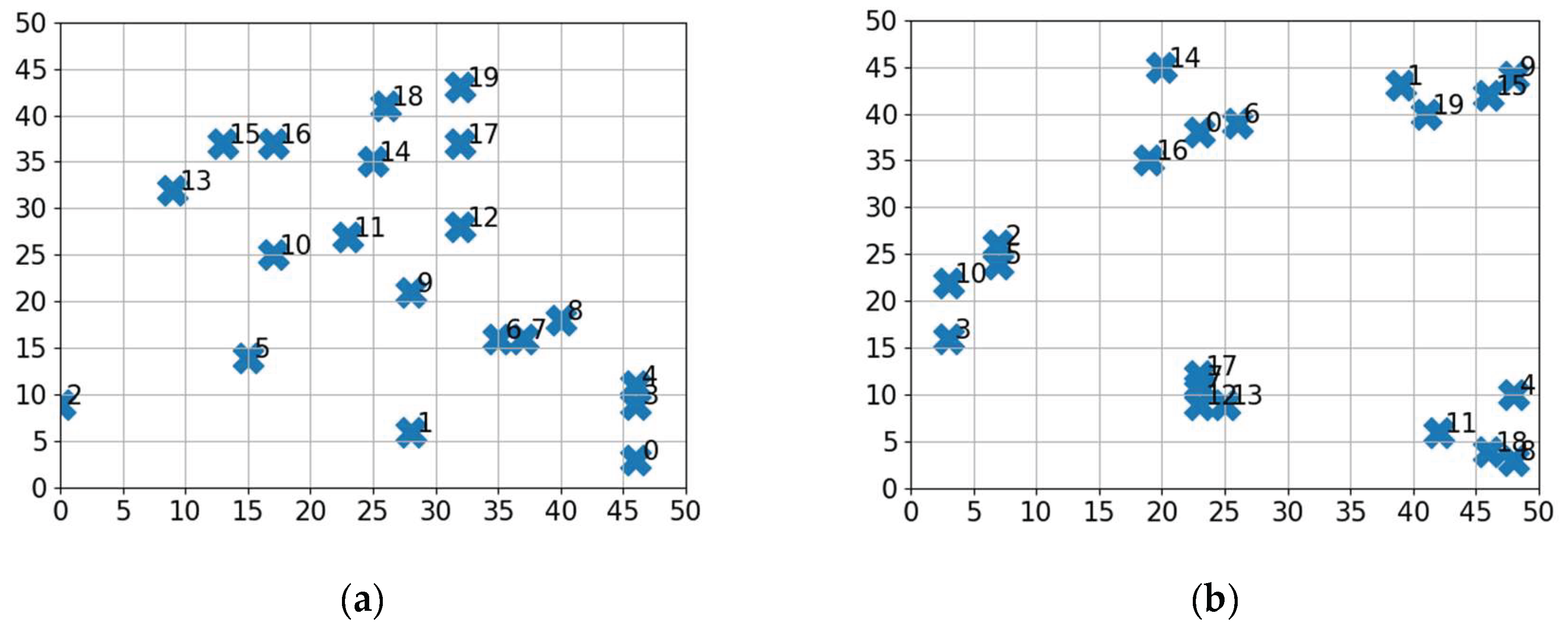
Figure 2.
Mean of RMSEs and W10s measured in the sample fields with random deployment and N = 10: (a) RMSE measured with B = 6; (b) RMSE measured with B = 25; (c) W10 measured with B = 6; (d) W10 measured with B = 25.
Figure 2.
Mean of RMSEs and W10s measured in the sample fields with random deployment and N = 10: (a) RMSE measured with B = 6; (b) RMSE measured with B = 25; (c) W10 measured with B = 6; (d) W10 measured with B = 25.
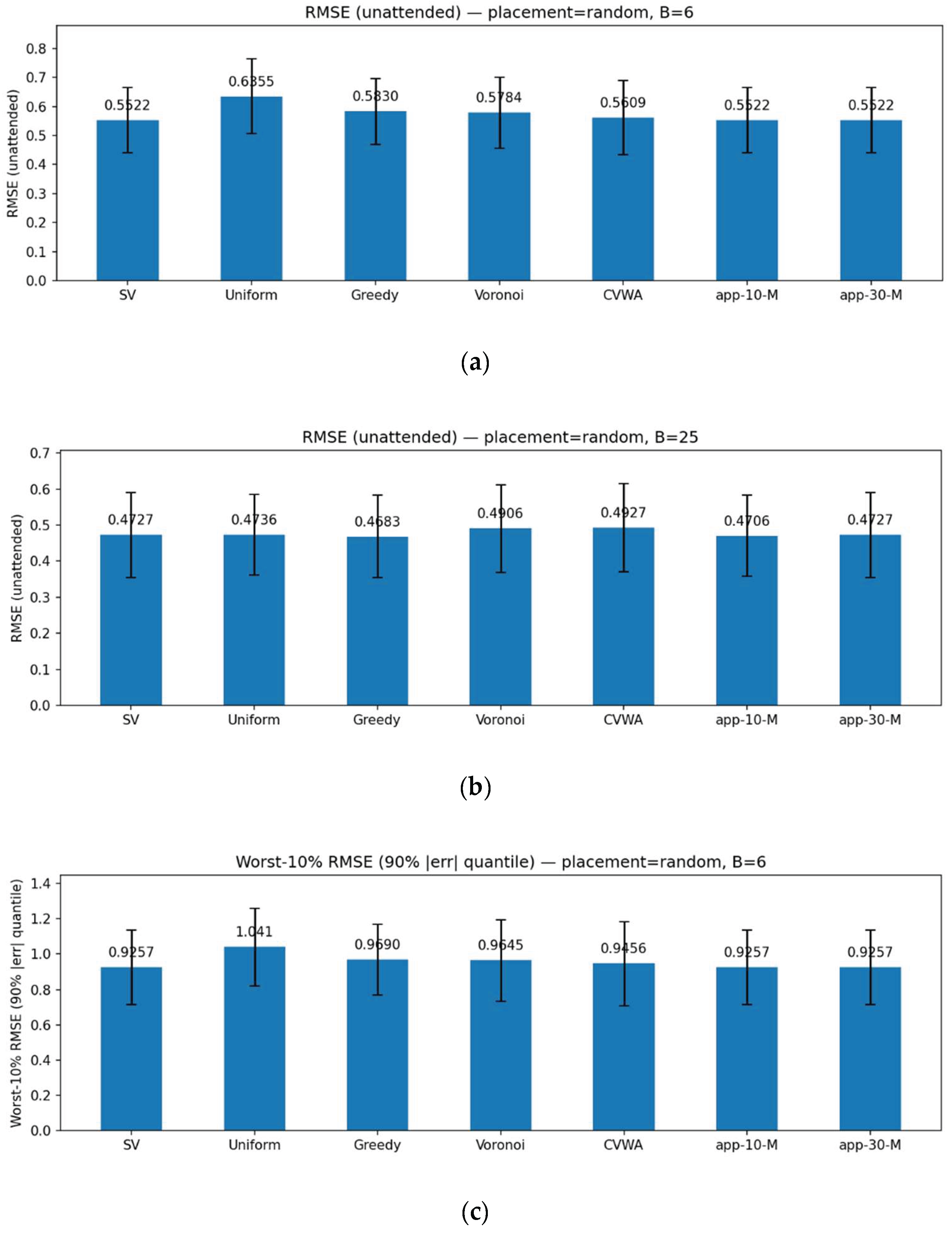
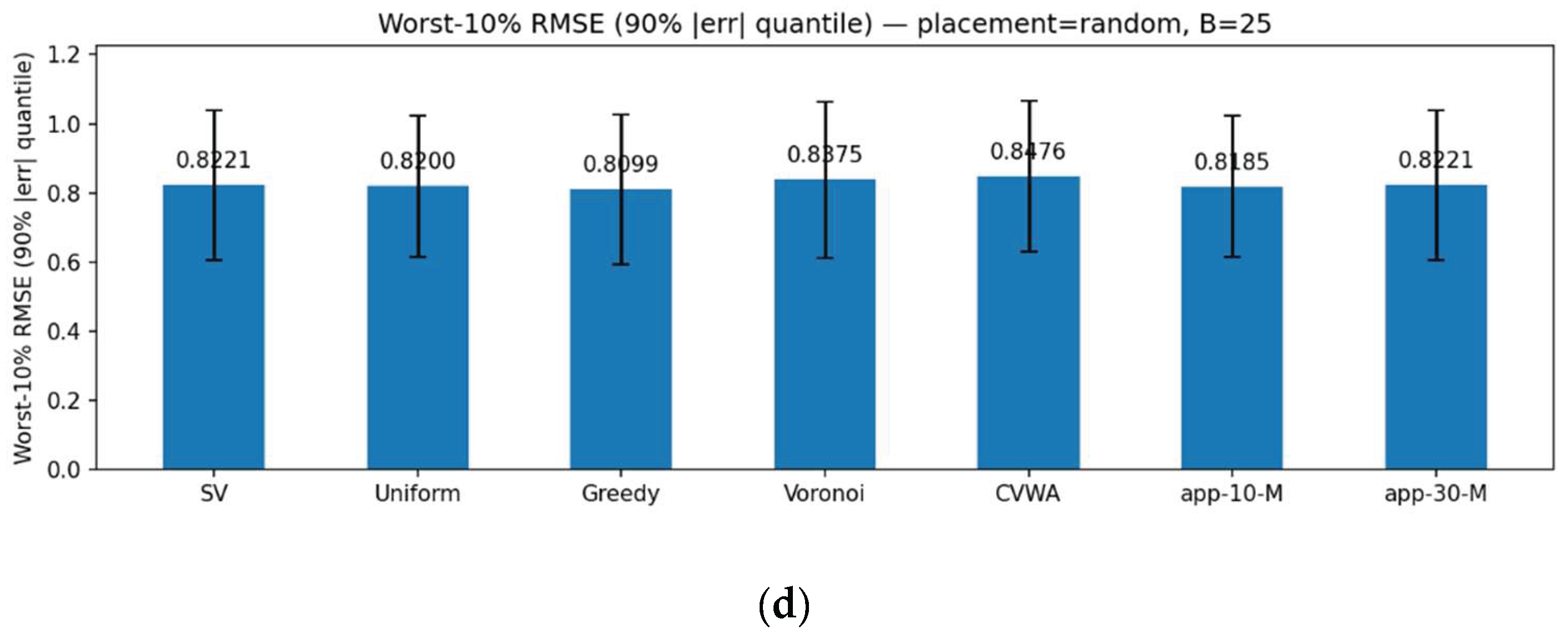
Figure 3.
Mean of RMSEs and W10s measured in the sample fields of clustered deployment and N = 10: (a) RMSE measured with B = 6; (b) RMSE measured with B = 25; (c) W10 measured with B = 6; (d) W10 measured with B = 25.
Figure 3.
Mean of RMSEs and W10s measured in the sample fields of clustered deployment and N = 10: (a) RMSE measured with B = 6; (b) RMSE measured with B = 25; (c) W10 measured with B = 6; (d) W10 measured with B = 25.
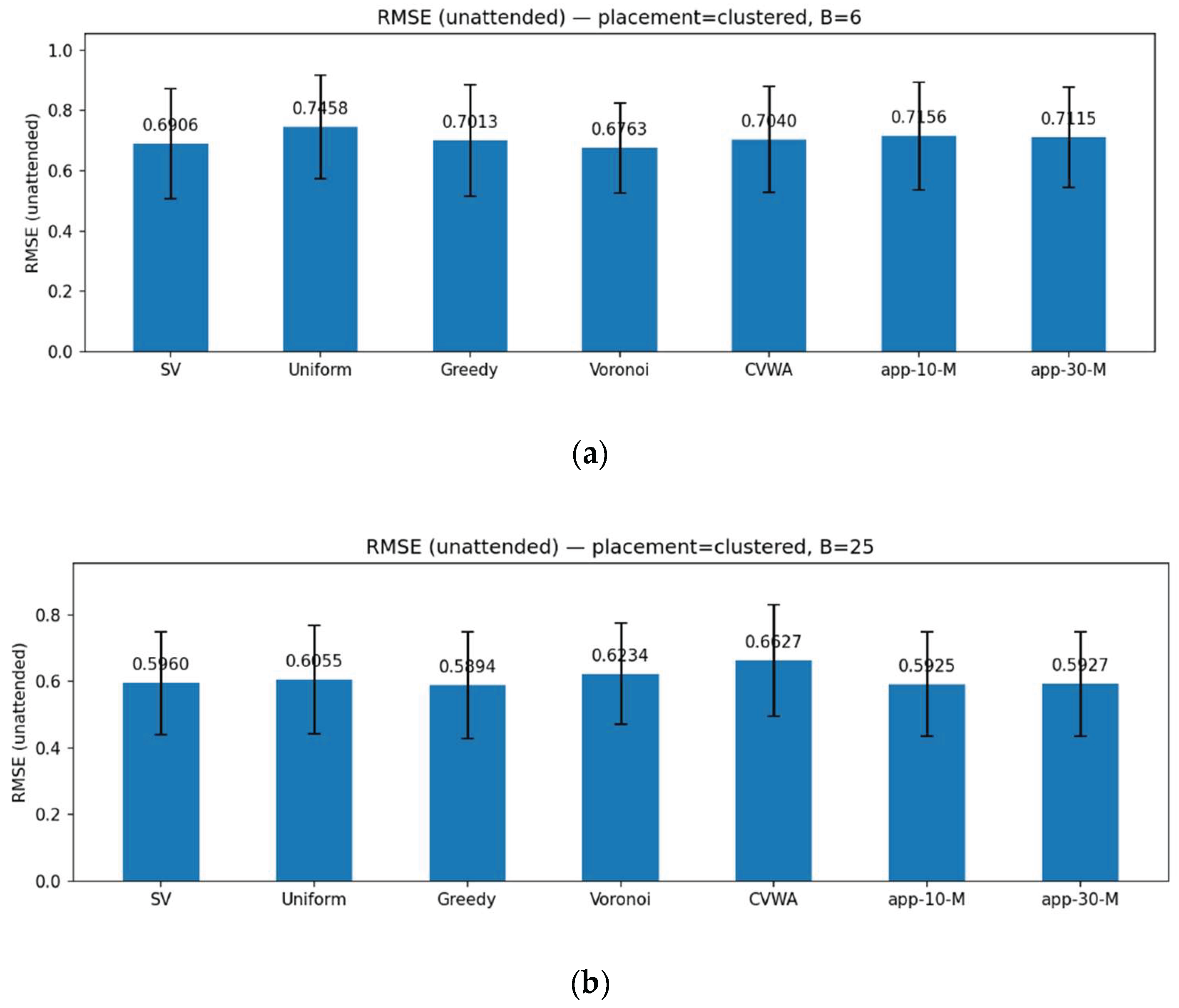
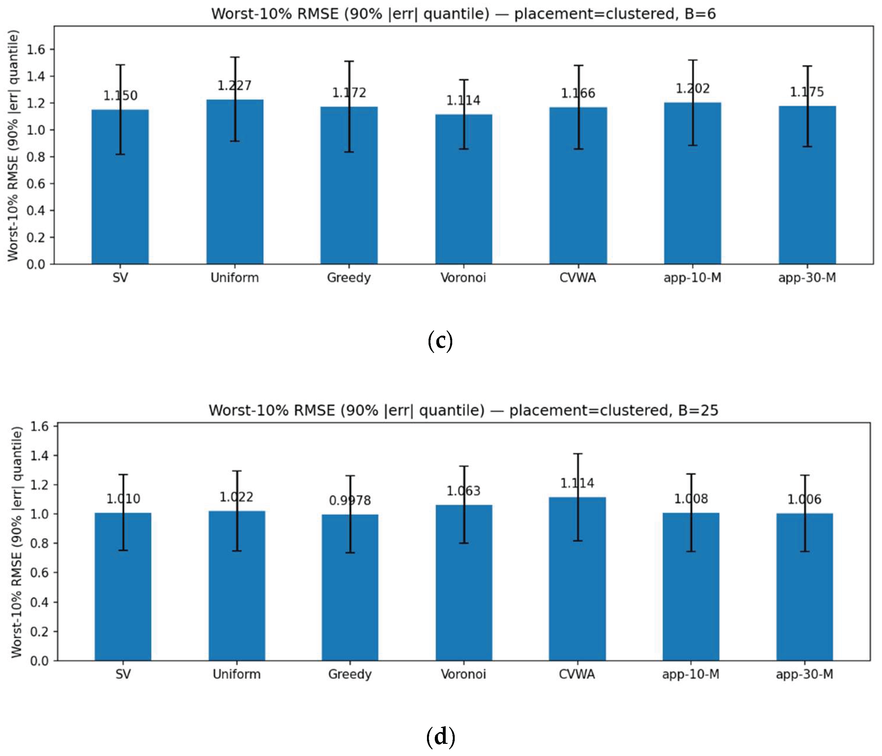
Figure 4.
Mean of RMSEs, W10s, and B-RMSEs measured in the sample fields of random deployment and N = 40: (a) RMSE measured with B = 30; (b) RMSE measured with B = 100; (c) W10 measured with B = 30; (d) W10 measured with B = 100; (e) B-RMSE measured with B = 30; (f) B-RMSE measured with B = 100.
Figure 4.
Mean of RMSEs, W10s, and B-RMSEs measured in the sample fields of random deployment and N = 40: (a) RMSE measured with B = 30; (b) RMSE measured with B = 100; (c) W10 measured with B = 30; (d) W10 measured with B = 100; (e) B-RMSE measured with B = 30; (f) B-RMSE measured with B = 100.
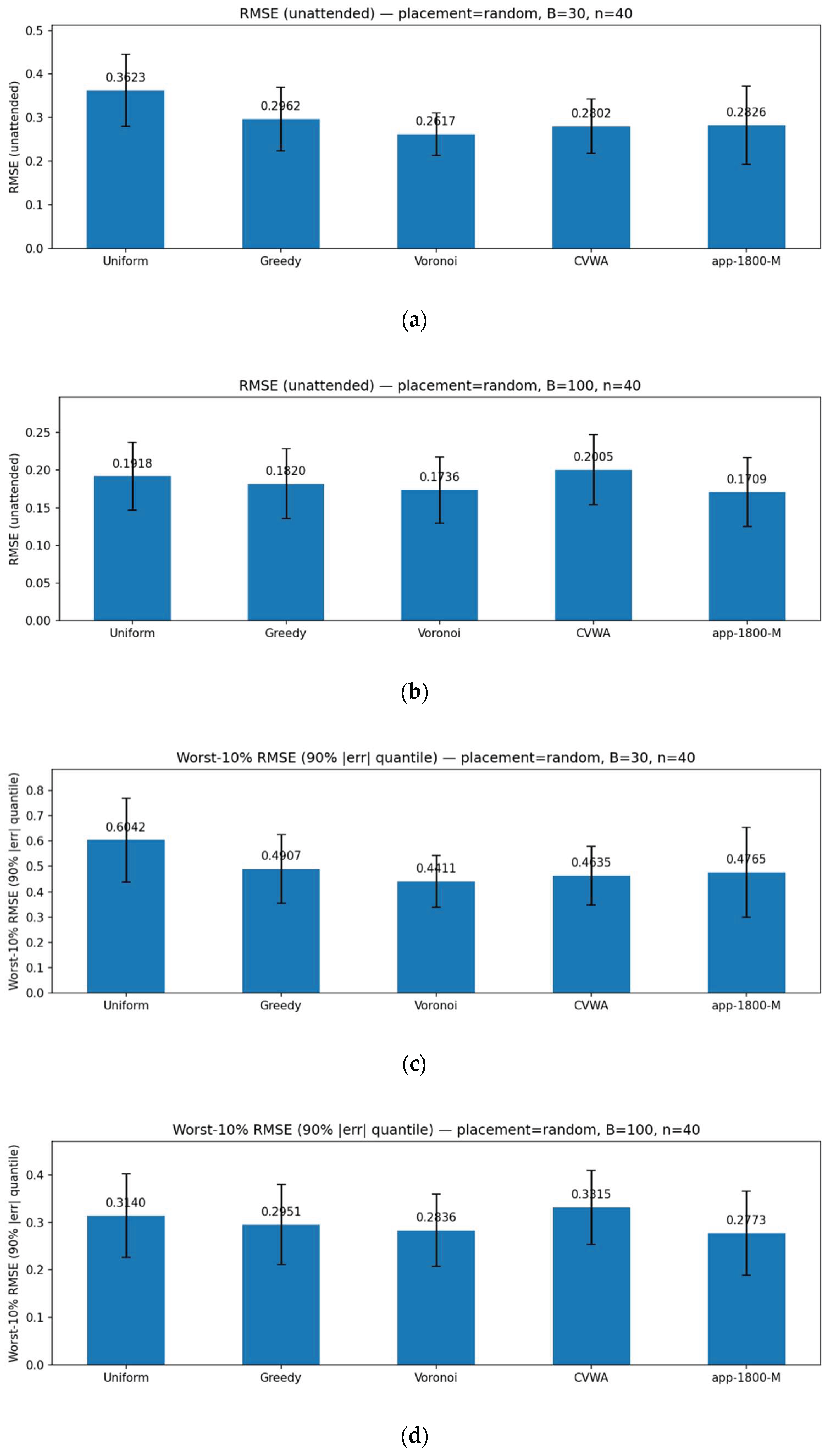
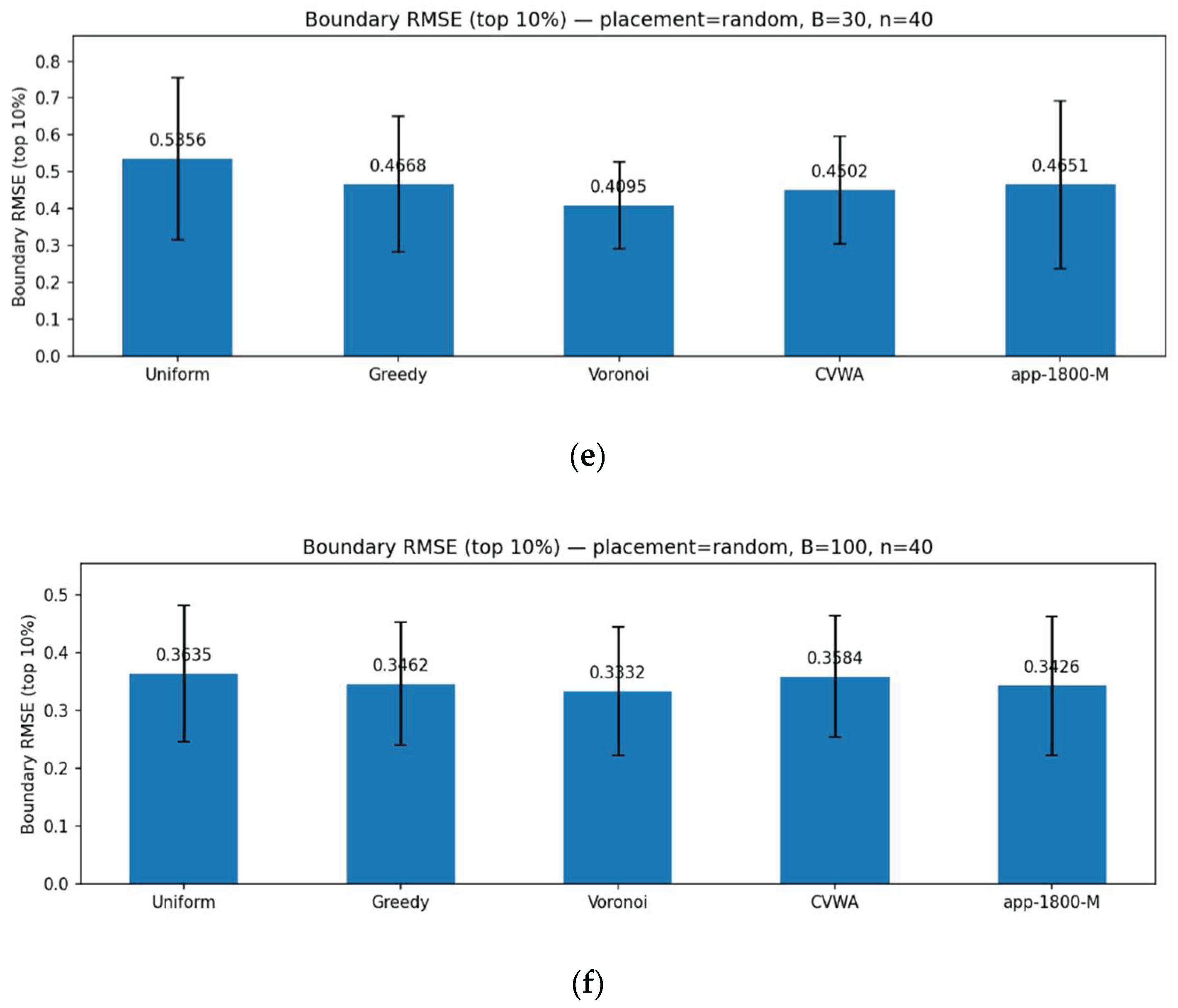
Figure 5.
Mean of RMSEs, W10s, and B-RMSEs measured in the sample fields of clustered deployment and N = 40; (a) RMSE measured with B = 30; (b) RMSE measured with B = 100; (c) W10 measured with B = 30; (d) W10 measured with B = 100; (e) B-RMSE measured with B = 30; (f) B-RMSE measured with B = 100.
Figure 5.
Mean of RMSEs, W10s, and B-RMSEs measured in the sample fields of clustered deployment and N = 40; (a) RMSE measured with B = 30; (b) RMSE measured with B = 100; (c) W10 measured with B = 30; (d) W10 measured with B = 100; (e) B-RMSE measured with B = 30; (f) B-RMSE measured with B = 100.
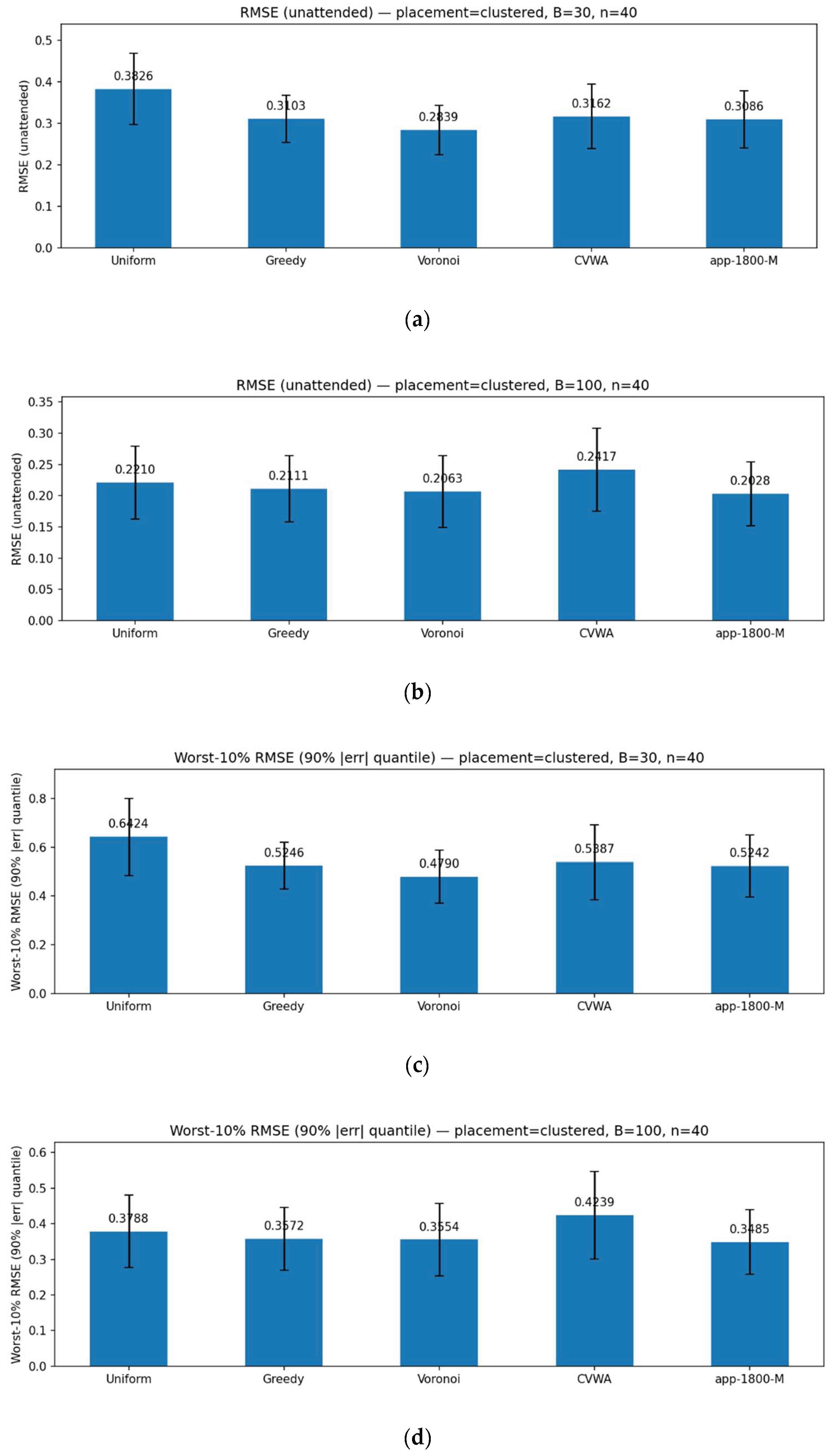
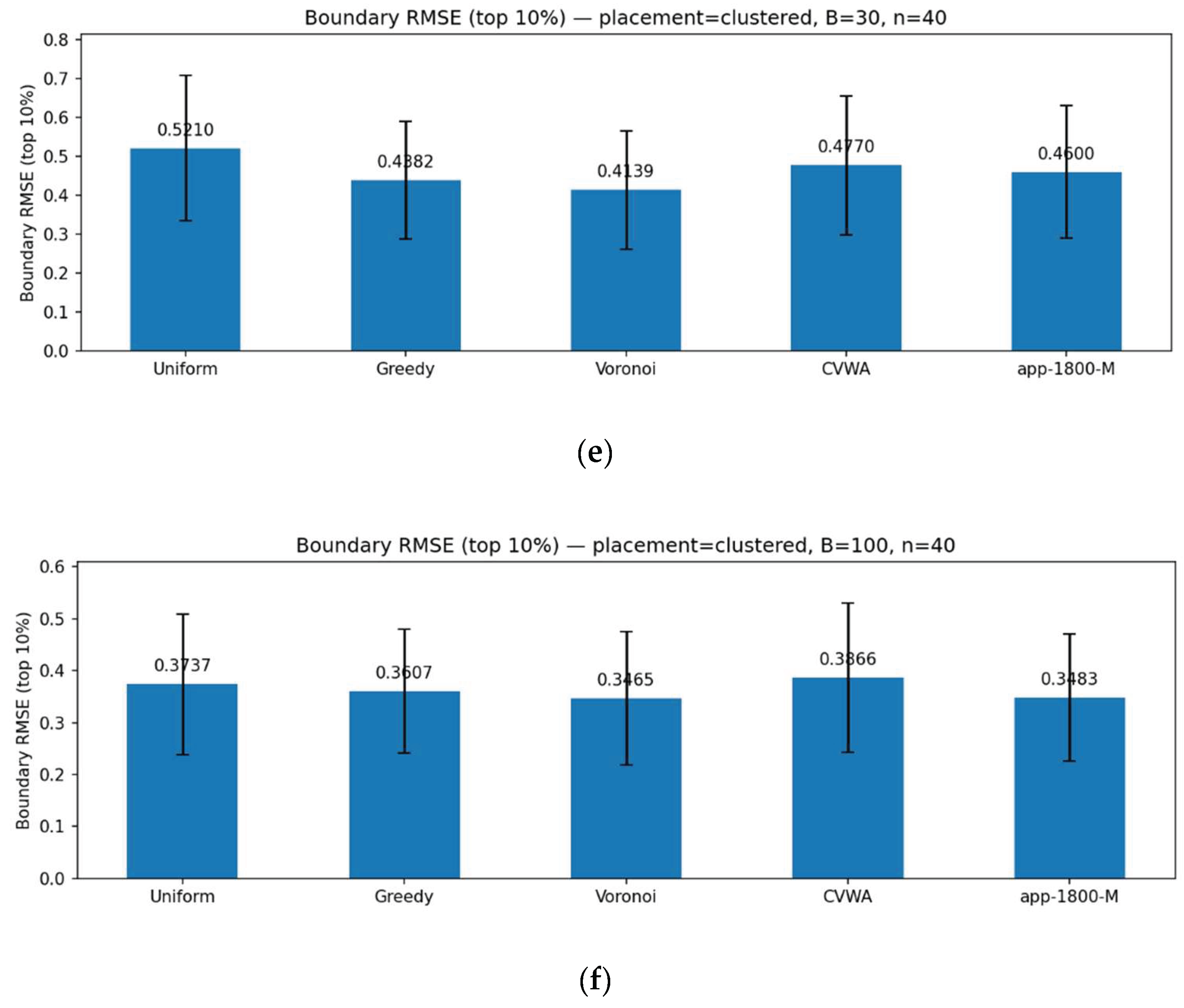
Figure 6.
MIs and WA-traces measured in the sample fields of random deployment and N = 10: (a) MI measured with B = 6; (b) MI measured with B = 25; (c) WA-trace measured with B = 6; (d) WA-trace measured with B = 25.
Figure 6.
MIs and WA-traces measured in the sample fields of random deployment and N = 10: (a) MI measured with B = 6; (b) MI measured with B = 25; (c) WA-trace measured with B = 6; (d) WA-trace measured with B = 25.
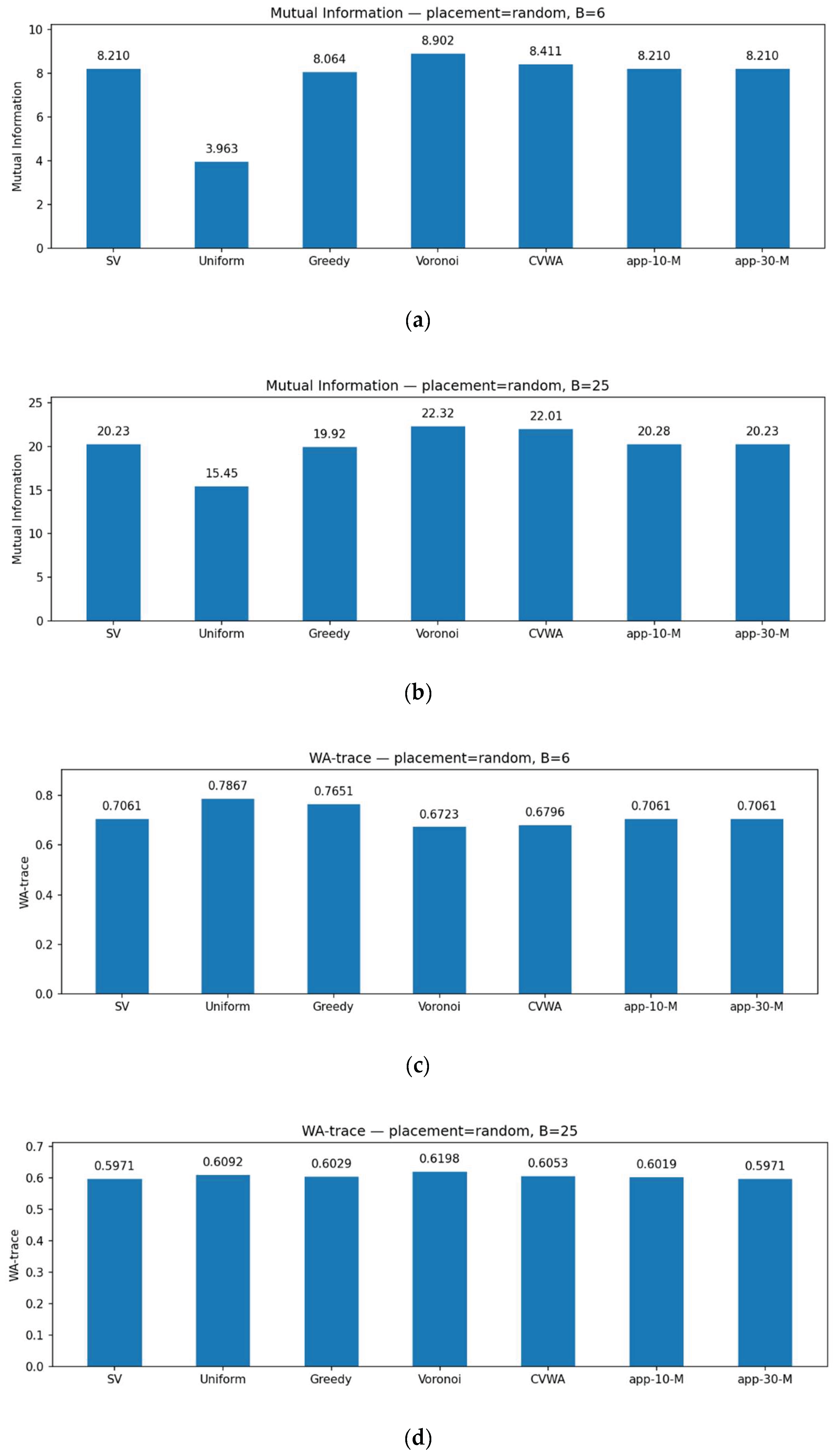
Figure 7.
MIs and WA-traces measured in the sample fields of clustered deployment and N = 10: (a) MI measured with B = 6; (b) MI measured with B = 25; (c) WA-trace measured with B = 6; (d) WA-trace measured with B = 25.
Figure 7.
MIs and WA-traces measured in the sample fields of clustered deployment and N = 10: (a) MI measured with B = 6; (b) MI measured with B = 25; (c) WA-trace measured with B = 6; (d) WA-trace measured with B = 25.
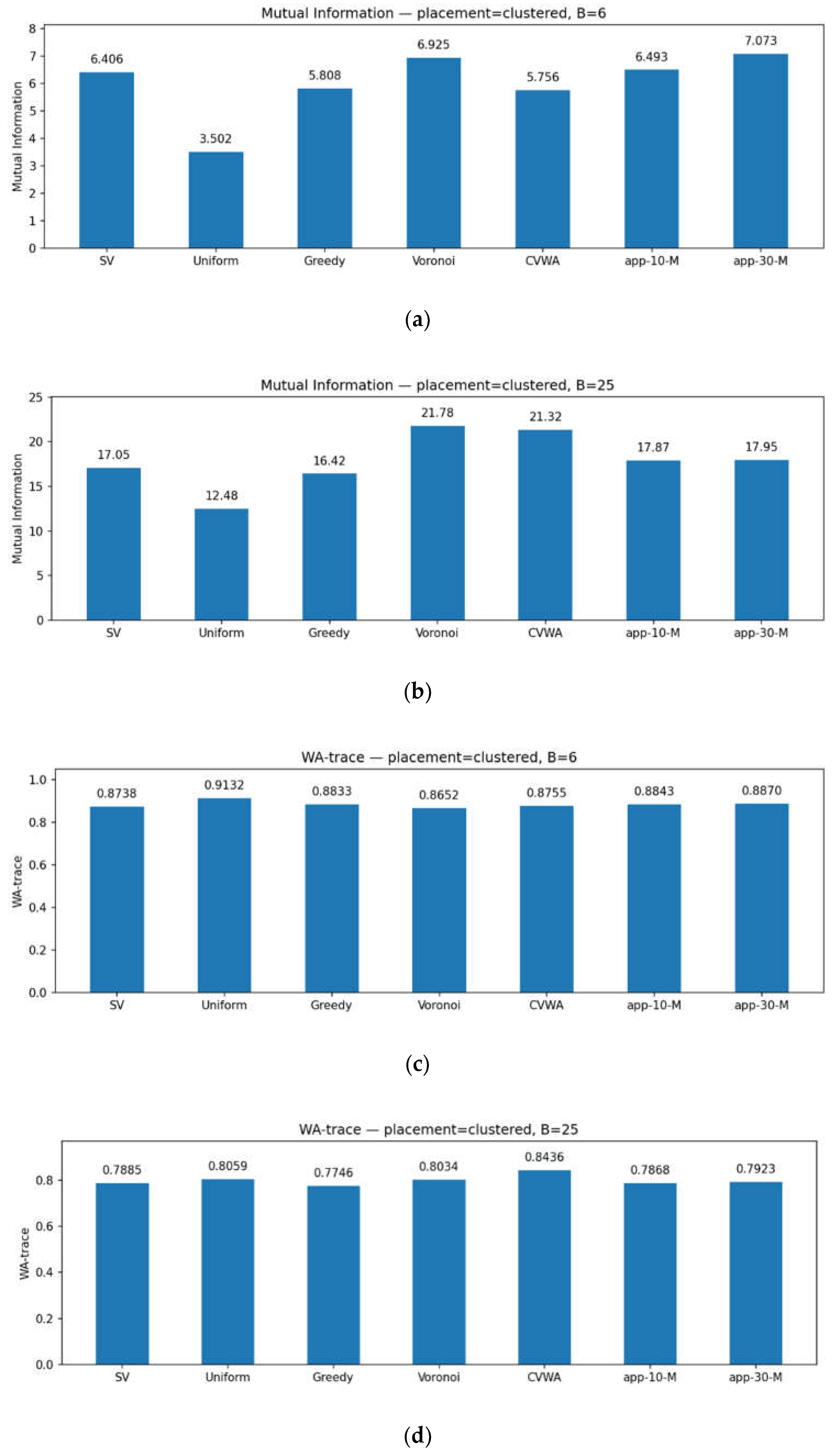
Figure 8.
MIs and WA-traces measured in the sample fields of random deployment and N = 40: (a) MI measured with B = 30; (b) MI measured with B = 100; (c) WA-trace measured with B = 30; (d) WA-trace measured with B = 100.
Figure 8.
MIs and WA-traces measured in the sample fields of random deployment and N = 40: (a) MI measured with B = 30; (b) MI measured with B = 100; (c) WA-trace measured with B = 30; (d) WA-trace measured with B = 100.
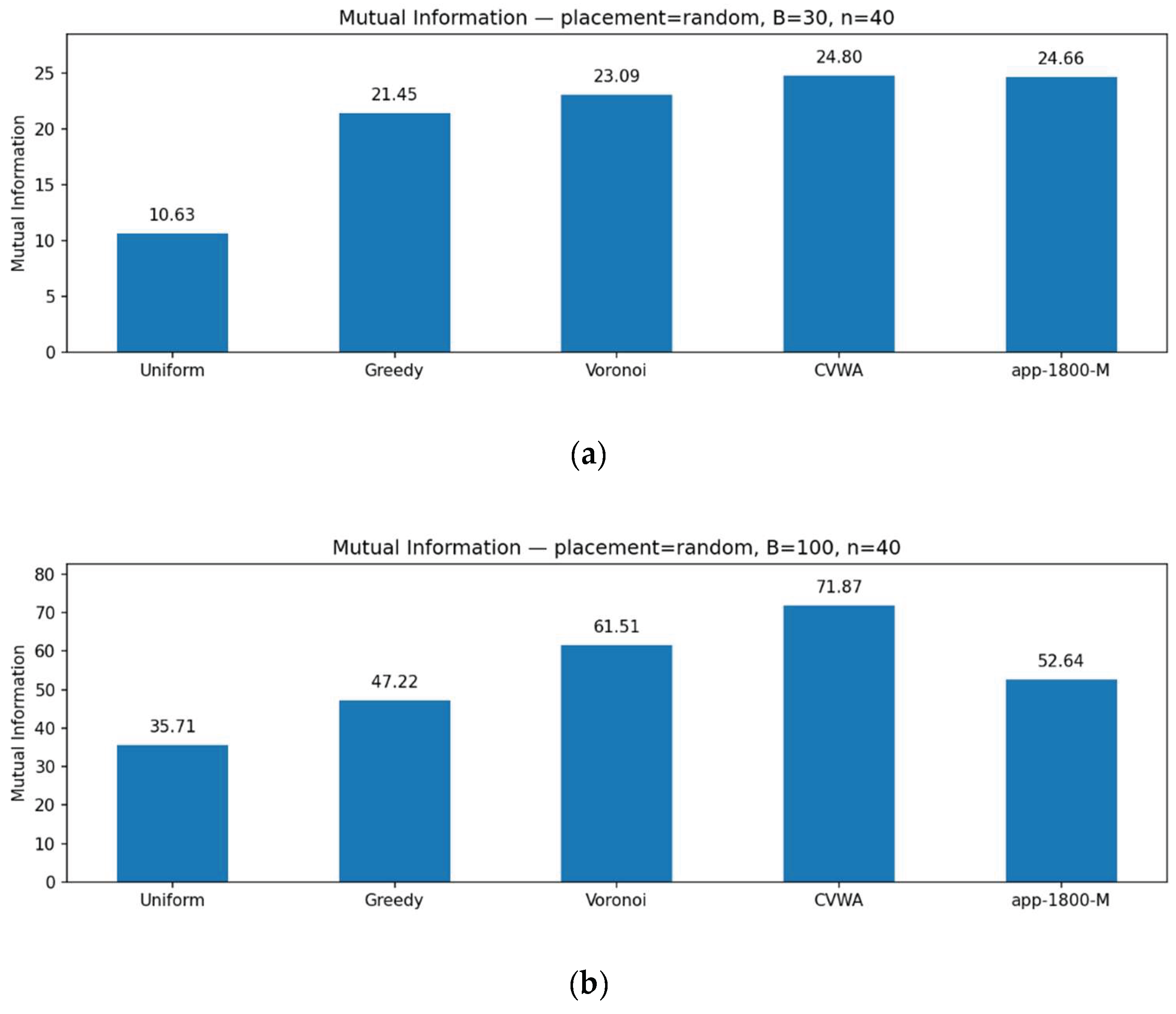
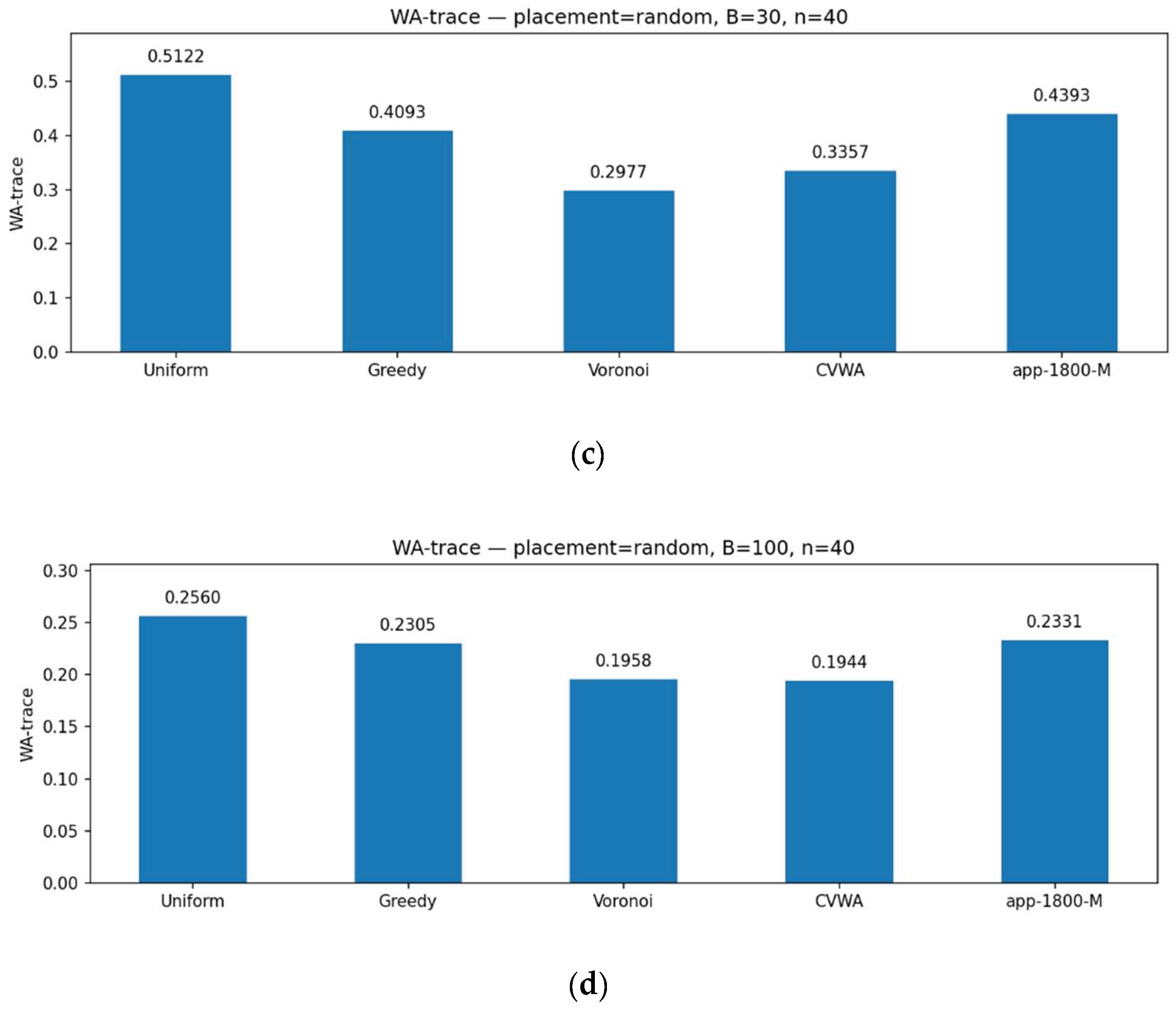
Figure 9.
MIs and WA-traces measured in the sample fields of clustered deployment and N = 40: (a) MI measured with B = 30; (b) MI measured with B = 100; (c) WA-trace measured B = 30; (d) WA-trace measured with B = 100.
Figure 9.
MIs and WA-traces measured in the sample fields of clustered deployment and N = 40: (a) MI measured with B = 30; (b) MI measured with B = 100; (c) WA-trace measured B = 30; (d) WA-trace measured with B = 100.
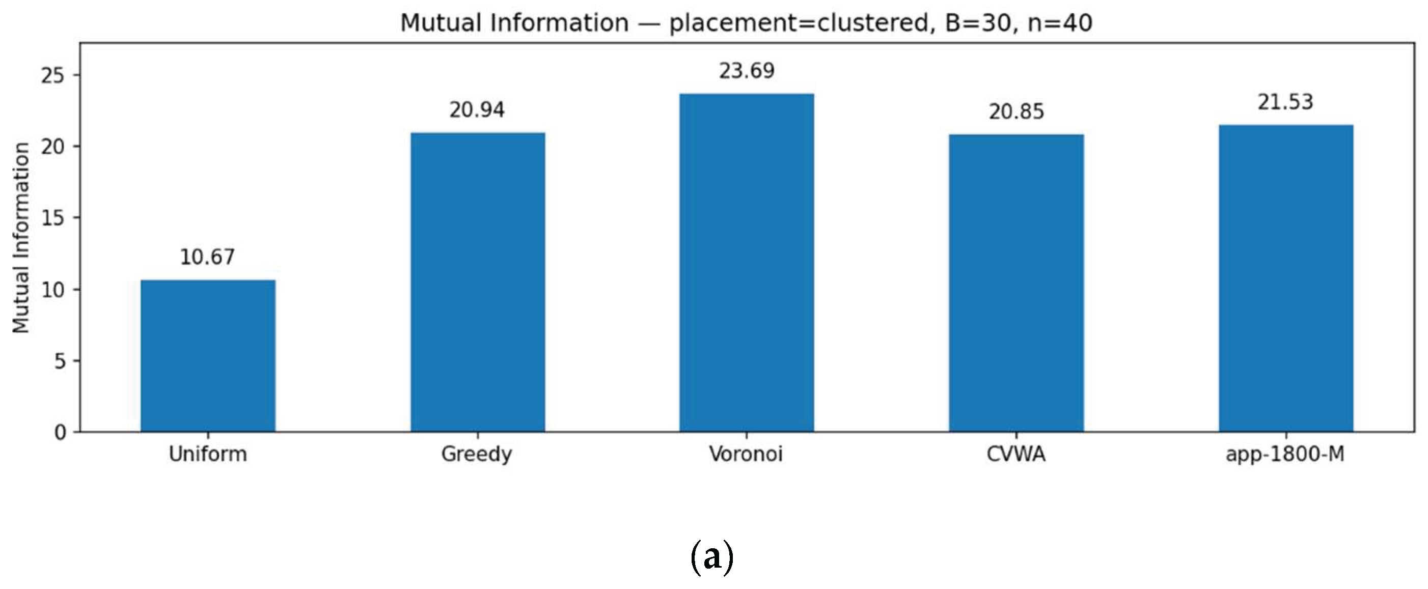
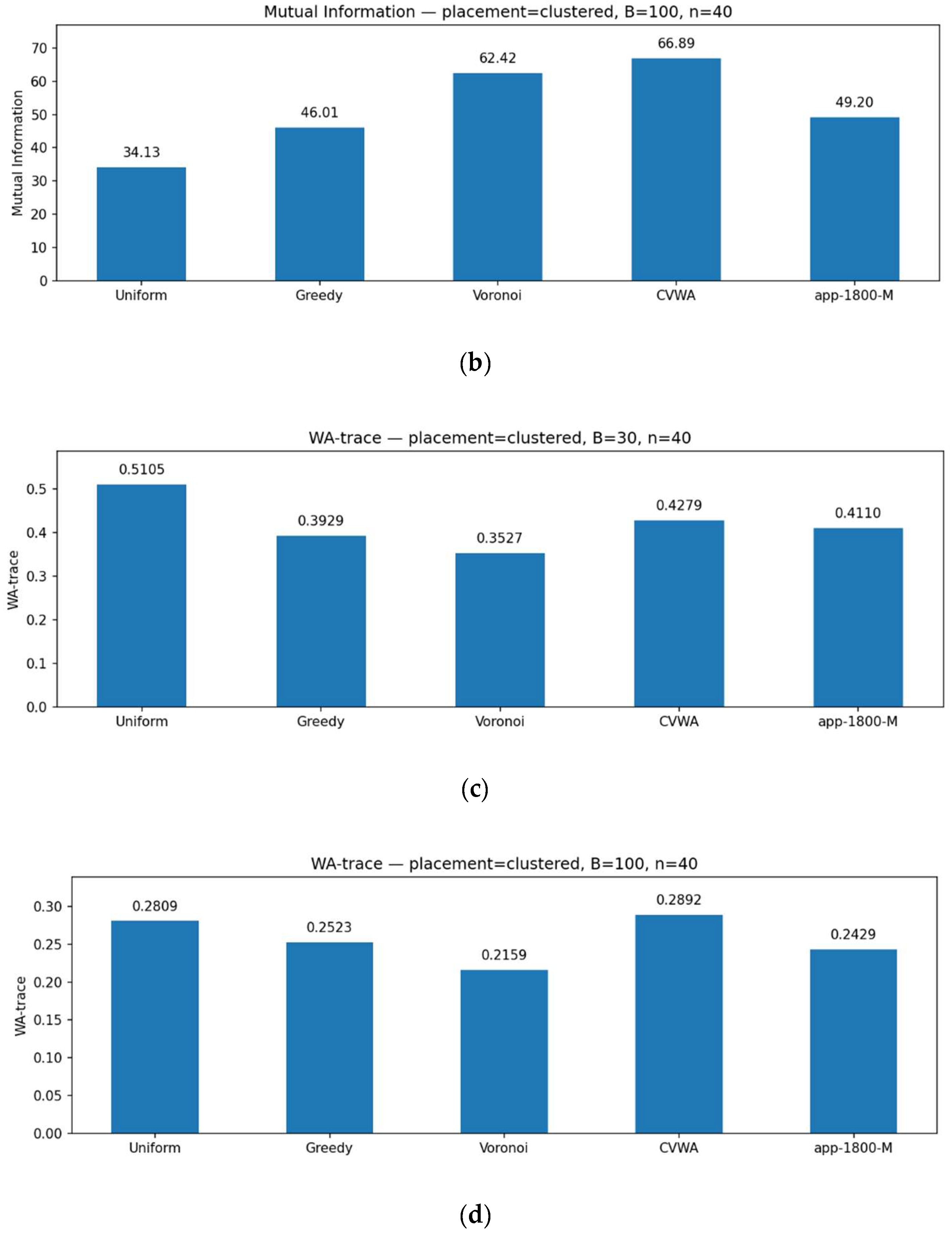

Table 1.
Experimental parameters.
| Item | Settings | |
|---|---|---|
| Field grid size | 50 × 50 | |
| α in the covariance model given in (4) | 0.3 | |
| Sensor deployments | random/clustered | |
| Number of samples used for finding the optimal mk | 20 | |
| Bit budgets (B) | N = 10 | 6, 25 |
| N = 40 | 30, 100 | |
| Sample budgets for stratified sampling (M) | N = 10 | 10, 30 |
| N = 40 | 1800 | |
| Number of clusters for the clustered sensor deployments | N = 10 | 3 |
| N = 40 | 8 | |
Table 2.
Efficiency consistency and execution time of the approximation.
| N | Deployment | M | Time (seconds) | v(S) | εeff (%) | |
|---|---|---|---|---|---|---|
| 10 | random | 10 | 8 | 229.996 | 230.071 | 0.0326 |
| 30 | 21 | 230.155 | 0.0365 | |||
| clustered | 10 | 7 | 208.061 | 206.987 | 0.5189 | |
| 30 | 19 | 206.850 | 0.0662 | |||
| 40 | random | 1800 | 1063 | 806.703 | 806.778 | 0.0093 |
| clustered | 1800 | 1030 | 732.363 | 732.912 | 0.0749 |
Table 3.
The best and 2nd best performing allocation methods in N = 10. Hyphen in ‘2nd best’ field implies two methods share the top rank with identical results in ‘Best’ category. ‘App.’ indicates approximation variants of SV.
Table 3.
The best and 2nd best performing allocation methods in N = 10. Hyphen in ‘2nd best’ field implies two methods share the top rank with identical results in ‘Best’ category. ‘App.’ indicates approximation variants of SV.
| Deployment | B | Metric | Best | 2nd Best |
|---|---|---|---|---|
| random | 6 | RMSE | SV, App. | - |
| B-RMSE | SV, App. | - | ||
| W10 | SV, App. | - | ||
| MI | Voronoi | CVWA | ||
| WA-trace | Voronoi | CVWA | ||
| 25 | RMSE | Greedy | App. | |
| B-RMSE | App. | Greedy | ||
| W10 | Greedy | App. | ||
| MI | Voronoi | CVWA | ||
| WA-trace | SV, App | - | ||
| clustered | 6 | RMSE | Voronoi | SV |
| B-RMSE | Voronoi | Greedy | ||
| W10 | Voronoi | SV | ||
| MI | App. | Voronoi | ||
| WA-trace | Voronoi | SV | ||
| 25 | RMSE | Greedy | App. | |
| B-RMSE | App. | Greedy | ||
| W10 | Greedy | App. | ||
| MI | Voronoi | CVWA | ||
| WA-trace | Greedy | App. |
Table 4.
The best and 2nd best performing allocation methods in N = 40.
| Deployment | B | Metric | Best | 2nd Best |
|---|---|---|---|---|
| random | 30 | RMSE | Voronoi | CVWA |
| B-RMSE | Voronoi | CVWA | ||
| W10 | Voronoi | CVWA | ||
| MI | CVWA | App. | ||
| WA-trace | Voronoi | CVWA | ||
| 100 | RMSE | App. | Voronoi | |
| B-RMSE | Voronoi | CVWA | ||
| W10 | App. | Voronoi | ||
| MI | CVWA | Voronoi | ||
| WA-trace | CVWA | Voronoi | ||
| clustered | 30 | RMSE | Voronoi | App. |
| B-RMSE | Voronoi | Greedy | ||
| W10 | Voronoi | App. | ||
| MI | Voronoi | CVWA | ||
| WA-trace | Voronoi | Greedy | ||
| 100 | RMSE | App. | Voronoi | |
| B-RMSE | Voronoi | App. | ||
| W10 | App. | Voronoi | ||
| MI | CVWA | Voronoi | ||
| WA-trace | Voronoi | App. |
Disclaimer/Publisher’s Note: The statements, opinions and data contained in all publications are solely those of the individual author(s) and contributor(s) and not of MDPI and/or the editor(s). MDPI and/or the editor(s) disclaim responsibility for any injury to people or property resulting from any ideas, methods, instructions or products referred to in the content. |
© 2026 by the authors. Licensee MDPI, Basel, Switzerland. This article is an open access article distributed under the terms and conditions of the Creative Commons Attribution (CC BY) license (http://creativecommons.org/licenses/by/4.0/).
Copyright: This open access article is published under a Creative Commons CC BY 4.0 license, which permit the free download, distribution, and reuse, provided that the author and preprint are cited in any reuse.


