

Submitted:
31 May 2026
Posted:
02 June 2026
You are already at the latest version
Abstract
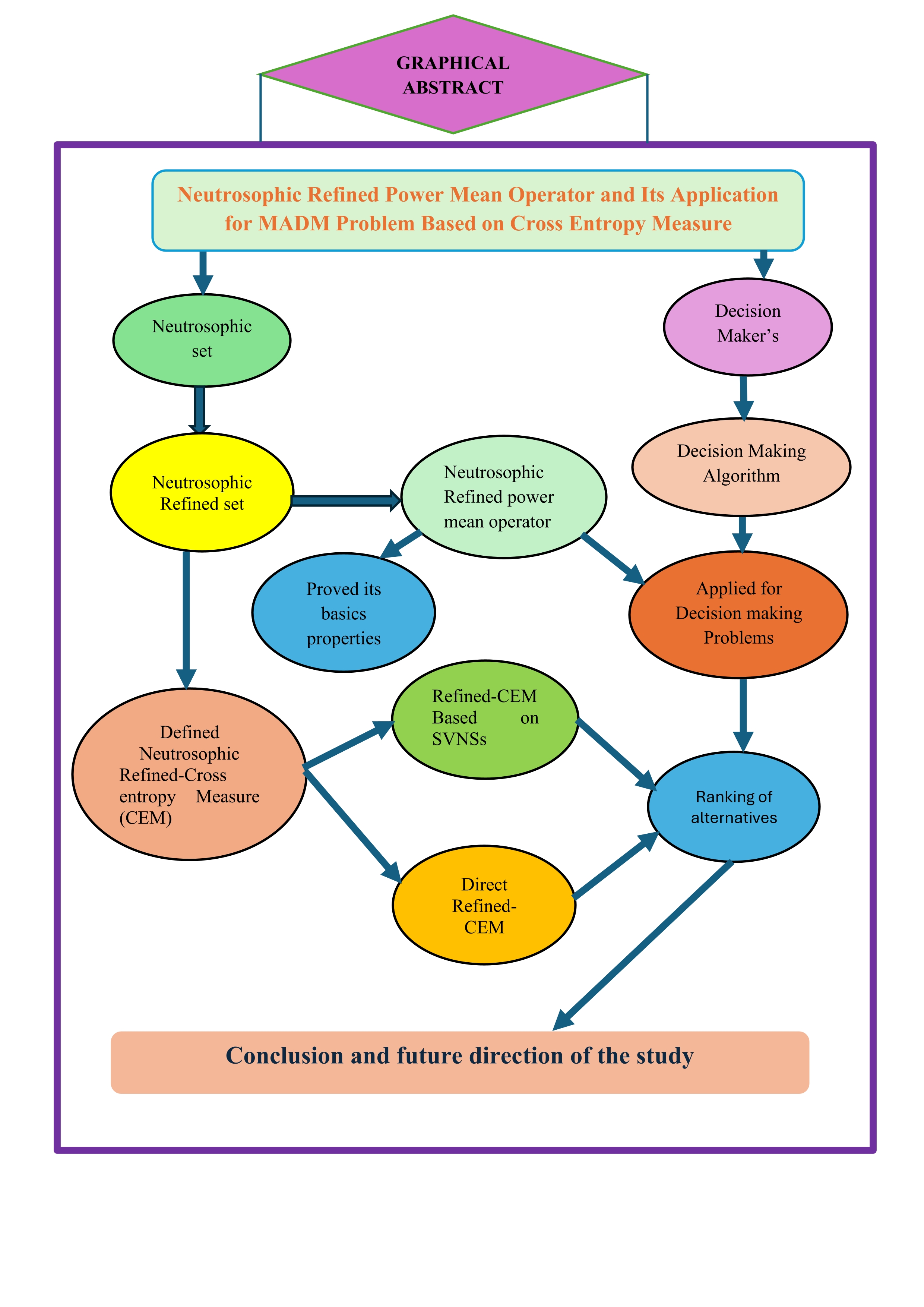
In real-world decision-making, constructing mathematical models is often difficult because the data are incomplete, uncertain, or even contradictory. The neutrosophic refined set provides a robust and flexible approach for effectively handling and representing these types of uncertainties. Various studies have highlighted its significant applications in decision making. In this study, a power mean operator is introduced to aggregate multiple Neutrosophic Refined Sets (NRSs) into a Single-Valued Neutrosophic Set (SVNs). The core mathematical properties of the newly introduced neutrosophic refined power mean operator are established. Moreover, two categories of neutrosophic refined cross-entropy measures are presented: one adapted from the SVNs-cross-entropy measure, and the other specifically formulated for neutrosophic refined sets. By employing the defined measures, an innovative decision making strategy is developed under the neutrosophic refined set environment. To demonstrate the effectiveness and practical relevance of the grounded strategy a numerical example based on the selection of an educational stream is solved.
Keywords:
neutrosophic set
; neutrosophic refined sets
; MADM
; neutrosophic refined power mean operator
; cross entropy measure
1. Introduction
Multi-Attribute Decision Making (MADM) denotes a decision process in which the optimal alternative is determined from a collection of feasible options considering multiple, potentially conflicting, criteria. Because decision-making information is frequently uncertain and incomplete, selecting the most suitable alternative becomes a challenging task. Zadeh was the first to formulate the Fuzzy Set (FS) [1], incorporating a degree of membership for all elements. Since then, numerous researchers have applied fuzzy set theory to various decision-making problems [2,3,4]. Later, Krassimir Atanassov [5] extended the concept of FS by introducing the Intuitionistic Fuzzy Set (IFS), which incorporates an independent degree of non-membership. IFSs have also been utilized in a wide range of decision-making scenarios [6,7]. Despite their broad applicability, FSs and IFSs are insufficient for modeling situations where the indeterminacy function (I-function) has no dependence on either the membership function (T-function) or the non-membership function (F-function). In real-world decision-making processes, indeterminacy inherently arises due to incomplete and imprecise information. To address this limitation, Smarandache [8] proposed the Neutrosophic Set (NS), in which three mutually independent functions T-function, I-function, and F-function are defined over the interval . Subsequently, wang et al. [9] introduced the Single Valued NS (SVNS) as a particular case of the NS framework, where each membership component assumes values from .
Over time, this concept has proven to be effective when applied in numerous fields and practical contexts [10,11,12,13,14,15,16]. Later, the neutrosophic framework was expanded to include interval neutrosophic sets (INS) [17], in which uncertainty is described using interval-based T-, I-, and F- function. Several studies have explored applications of INSs in different domains [18,19,20,21,22,23,24]. Later, the neutrosophic framework was expanded to include INS [17], in which uncertainty is described using interval-based components of T-, I-, and F-function. Several studies have explored the applications of INSs in different domains [18,19,20,21,22,23,24].
Motivation of the Study
In particular cases, a mathematical framework that can represent repeated occurrences of elements is needed, such as the symptoms of a patient measured over different time intervals. To deal with this kind of situation, we use the concept [25]. The concept of a multiset can be found in [26]. Later, several researchers have discussed more properties and applications of multiset [27,28,29]. The concept of fuzzy bags was formally defined by Baowen et al. [30] in 1998. Miyamoto [31] defined the concepts of multisets in fuzzy environment in 2001. Later, Rocacher [32] applied fuzzy bags to build up flexible query. Shinoj and Sunil [33] developed Intuitionistic Fuzzy mMltisets (IFMs) as an extension of fuzzy multisets and proposed various associated operations. In [33] Shinoj and Sunil employed the IFMs in medical diagnosis problem. In 2013, Smarandache [34] introduced the concept of a refined NS (RNS) by further developing the components of NS.
Subsequently, numerous researchers have applied NRSs to MADM problems using various approaches [35,36,37,38,39,40]. Cross entropy measure is a popular divergence measure in recent literature that calculates the divergence of any variable from other variables. The combination of cross entropy measure techniques with several decision-making environments by a lot of researchers are stated in Table 1.
Several researchers discussed more excellent results based on the fuzzy multisets [52,53,54] and intuitionistic fuzzy multisets [55,56,57,58,59,60,61].
However, NRS is a mathematical tool to express an element by the repeated membership, indeterminacy, and falsity degrees. Table 2 shows that few studies have been performed in the environment of NRSs. However, no study has been reported in the literature so far with cross entropy measure in NRS environment despite significant advantages of cross entropy measure in the decision-making field.
Motivated by these innovative ideas, we formulated a cross-entropy measure within the NRS environment and introduced a MADM approach applicable to the educational field.
Contribution of the Study
The primary objective of this research is to develop a methodology to identify the most suitable option among a set of feasible alternatives. To accomplish this objective within a decision-making framework, an aggregation operator is first formulated in general, and its crucial properties are rigorously established. Furthermore, a analysis is performed to show the stability and effectiveness of the grounded operator.
The principal contributions of this research are summarized as:
- A novel concept of the power mean operator is introduced within the neutrosophic refined set (NRS) framework.
- We systematically proved its essential mathematical properties.
- Two distinct formulations of the CEM are proposed in the NRS Setting to quantify the degree of dissimilarity between two NRSs.
- An MADM framework based on the proposed CEM is introduced to address issues related to DM-problems involving uncertainty and imprecision in an efficient manner.
- Solve a real-world MADM problem using the proposed method to demonstrate its practical applicability in the current context.
- A analysis isperformed to explore the effect of varying the parameter q on the decision-making outcomes of the operator.
Structure of This Study
The general structure of the remaining content is presented as follows. Section-2 covers the foundational concepts of NS, SVNS, and NRS, along with basic operations on NRS. This section also introduces the neutrosophic refined power mean operator, establishes its key properties, and discusses several special cases. Section 3 presents two types of NRS-based CEM and examines their main properties. Section 4 introduces an MADM approach utilizing the power mean operator to solve MADM g problems within the NRS framework. Section 5 presents a numerical illustration to assess the of the approach, while Section 6 summarizes the study and outlines the concluding observations and future research directions.
2. Preliminaries
This section briefly discusses SVNS, and NRSs, along with a description of their fundamental set-theoretic operations.
Definition 1: SVNS [9]
Let represent a discourse universe that consists of elements (or objects), where each element in is denoted by , i.e., . An SVNS defined in is characterized by the T-function , the I-function , and the F-function . Each of these functions maps the elements of into the interval , that is,
Consequently, SVNS can be represented as
Since , , and take values in , and their sum lies:
For simplicity, a SVNS can be denoted as , which is referred to as a single-valued neutrosophic number (SVNN). Symbolically, it is represented in the form of an SVNN.
Example 1: Consider an SVNS defined in the universe . Then, can be represented as
Consequently, the corresponding SVNN is expressed as
Definition 2:NRS [34]
Assume that is a non-empty universe with elements denoted by . An NRS defined in is represented by and expressed as
Each of the sequences , , and is a mapping from to .
These sequences represent the T-function, the I-function, and the F-function, respectively.
Example 2: Assume that is a universe and consider as a NRS defined in . Then, can be written as
The operations of NRSs described in [34] are presented below:
- 1.
-
Inclusion of NRSsLet and be two NRSs defined in a universe . The inclusion relation holds if and only if, for every and each refinement index , the following conditions are satisfied:Example 3:Consider two NRSs and on defined as:From the inclusion condition above, it follows that .
- 2.
-
Equality of Two NRSsTwo NRSs and in are said to be equal, denoted by , if and only if for every and each ,
- 3.
-
Complement of an NRSsLet be an NRS defined on the universe . The complement of , denoted by , is defined by:Example 4: Let an NRS on be expressed as:Then, its complement is obtained as:
- 4.
-
Union of two NRSsLet and be two NRSs on the universe . They can be written asandThe union is defined byExample 5: Let usThen
- 5.
-
Intersection of two NRSsLet and be two NRSs on . Their intersection is defined by
2.1. Some Operation of NRSs [34]
Assume that and are two NRss defined in the universe . For every and each , the operations are described as follows:
- 1.
- Additive operation
- 2.
- Multiplicative operation
- 3.
- Scalar multiplication
- 4.
- Scalar exponentiation
Definition 3: Neutrosophic Refined Power Mean Operator
Let denote the family of all neutrosophic refined sets on , and let denote the class of all SVNSs on . Suppose that
is a mapping defined on . Then is called the neutrosophic refined power mean operator, and it is defined as
where is a real parameter and p is a positive integer. Here, , , and denote the refined T-function, I-function, and F-function values of the neutrosophic refined set .
Lemma 1. For the operator defined above,
Proof. For every and ,
Hence,
Thus,
Therefore,
Similarly,
Hence,
which completes the proof.
Special Cases.
Case 1.
For , Eq. (1) simplifies to
Expression (2) is referred to as the arithmetic mean transformation function (AMTF).
Case 2.
For , Eq. (1) reduces to
Equation (3) is known as the geometric mean transformation function (GMTF).
Proof.
To analyze the behavior of Eq. (1), we rewrite it in exponential form:
By expressing each component logarithmically, we obtain
Taking the limit , L’Hospital’s rule yields
Finally, continuity of the exponential function provides
□
Case 3.
For , the expression in Eq. (1) generates a sequence of higher-order refined mean operators. Specifically, for we obtain the quadratic mean transformation function, for the cubic mean transformation function, and similarly for all larger values of q.
Case 4.The limit as
Without affecting generality, suppose that the refined membership values are sorted in non-increasing sequence.
Then,
Because all normalized terms lie within and the largest element dominates as , we obtain
Equivalently,
3. Properties of Neutrosophic Refined Power Mean Operator
Property 1: Idempotency
If all refined T-function values , all refined I-function values , and all refined F-function values are constant, then the operator returns that same constant triple.
Proof. Assume that the refined membership sequences consist of identical values, i.e.,
Then each summation in the operator becomes
and similarly for the indeterminacy and falsity components. Thus,
Hence, the operator is idempotent, completing the proof.
Property 2: Monotonicity
Let
and
be two NRSs defined on .
Assume that componentwise, i.e.,
for every and . Then,
Proof. Since
raising both sides to the power q gives
Summing over i yields
and hence
Similarly, from and , we obtain
Combining (6)–(8), we conclude that
which proves the monotonicity of the operator.
Property 3: Boundedness
Let be any family of neutrosophic refined sets defined on the universe . For this collection, define the upper and lower neutrosophic bounds as
Then the following bound holds:
Proof.
From Properties 1 and 2, each component produced by the operator is bounded below by the corresponding component of and bounded above by the corresponding component of . Thus,
which directly yields
4. CEM for NRSs
Here, two distinct formulations are proposed to evaluate the CEM of NRSs. These formulations are developed by extending the concept of the CEM defined for SVNs, as introduced in [11]. For completeness, we first revisit the notion of cross-entropy within the framework of SVNs.
Definition 4: Single-valued neutrosophic CEM [11].
Let and be two SVNSs defined over the universe
The CEM between and is represented by
and is mathematically expressed as
Theorem 1:Single-valued neutrosophic CEM for any two SVNSs and meets the following conditions:
- if and only if
Definition 5: Neutrosophic Refined CEM
Let and be any two NRSs in . Then, the neutrosophic refined cross-entropy between and is defined as
Theorem 2:
Neutrosophic refined CEMfor any two NRSssatisfies the following properties:
- if and only if
Definition 6: Neutrosophic refined weighted CEM
Let and be two NRSs defined throughout the . Assume that each element is assigned a weight , forming the weight vector , where and . Under these assumptions, the weighted cross-entropy measure for and in the neutrosophic refined framework is defined as follows:
Theorem 3: The neutrosophic refined CEM for any two satisfies the following properties:
- if and only if
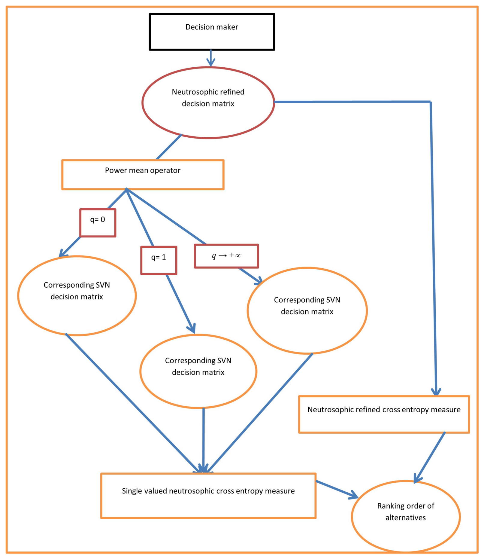
5. Cross Entropy Based MADM Strategy in NRS Environment Using Power Mean Operator
In this section, a systematic procedure is presented to identify the priority ranking of all available alternatives in the NRN framework. Let denote the collection of aspirant candidates. represent the set of evaluation attributes and be the set of alternatives available associated with each candidate.
The decision-maker evaluates each available alternative with respect to each criterion that is sufficient to evaluate the alternatives are denoted by employing . Moreover, the ideal performance levels of all criteria are determined by the decision-maker in the form of SVNN.
Based on the defined aggregation operators, the MADM Technique is implemented through the following steps:
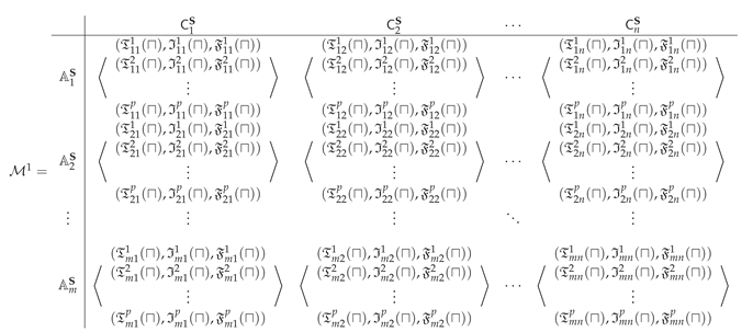
Step 1: Formulation of the decision matrix (D-Matrix) relates the candidates to attributes. The relationship between each candidate and each attribute expressed in terms of NRS information is organized in the following matrix (denoted by ):
Step 2: Construction of attributes–alternative D-Matrix
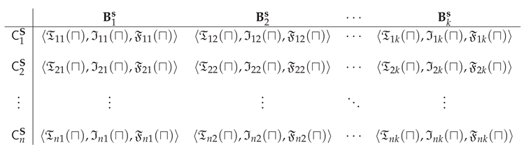
The association between each attribute and each available alternative is organized in the following form, represented by the matrix .
: Attributes versus alternatives SVN’s D-Matrix
Step 3. Convert NRSs to SVNSs
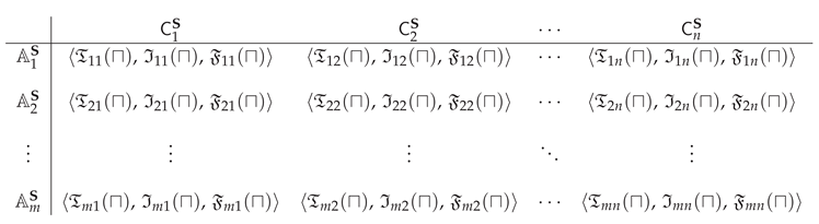
Using the neutrosophic power mean operator defined in Eq. (1), we convert NRSs in to SVNSs and produce in .
: Candidates versus attributes SVNSs D-Matrix
Step 4. Calculation of CE-measure values
We calculate the CE-measure values between and .
Step 5. Order the alternatives according to the results of the evaluation.
The available alternatives are prioritized according to the ascending values of the CE-measure. A lower CE-value indicates a more preferable available alternative.
Step 6. End
Figure 1.
Proposed decision-making procedure.
6. Example: Selection of an Appropriate Educational Stream
Drawing inspiration from [38], we consider an MADM problem related to selecting an appropriate educational stream for higher studies. Choosing the right path after completing the 10+2 level is often a challenge for students and their families. In this example, we determine the preference ranking of various streams for each student using a set of evaluative attributes (see Table 3).
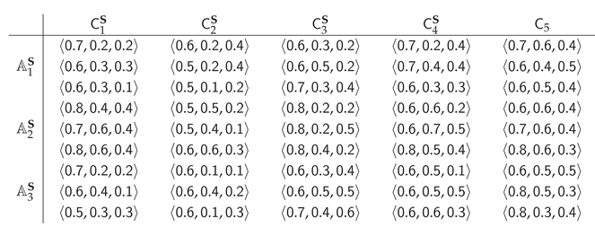
Step 1.Formulation of a D-Matrix between candidates and evaluation attributes.
The relationship between aspirant students and their corresponding attributes is modeled using NRSs, based on three mutually independent evaluations provided by a decision maker. The resulting triplet of relational values for each student is represented in .
The evaluation scores of the available alternatives with reference to the required attributes are represented using SVNSs. These SVNS-based assessments are arranged in the alternatives-versus-attributes decision matrix, denoted by .
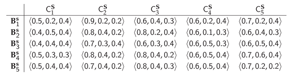
Step 3. Convert NRNs to SVNN
Using the neutrosophic power mean operator defined in Eq. (1) and different values of q, we obtain the following matrices.
When , the single valued decision matrix corresponding to the candidates versus attributes is represented in .
: Candidates versus attributes converted SVNS D-Matrix
When
: Candidates versus attributes converted SVNS D-Matrix
When
: Candidates versus attributes converted SVNS D-Matrix
Step 4. Calculation of cross entropy measure values
Using Eq. (9), we compute the cross-entropy values between and (see matrix ); and (see matrix ); and and (see matrix ). The resulting cross-entropy values are presented in the following table:
: Cross-entropy values between and
| Candidates | Mathematics Honors () | Physics Honors () | Engineering () | Computer Science () | Biochemistry () |
| 1.34 | 2.12 | 1.52 | 1.27 | 1.77 | |
| 2.26 | 1.54 | 1.59 | 1.39 | 1.46 | |
| 1.67 | 2.22 | 1.51 | 1.50 | 1.78 |
: Cross entropy values between and
| Candidates | Mathematics Honors () | Physics Honors () | Engineering () | Computer Science () | Biochemistry () |
| 1.41 | 2.06 | 1.18 | 1.42 | 1.62 | |
| 2.28 | 1.57 | 1.59 | 1.32 | 1.48 | |
| 1.68 | 2.22 | 1.34 | 1.58 | 1.78 |
: Cross entropy values between and
| Candidates | Mathematics Honors () | Physics Honors () | Engineering () | Computer Science () | Biochemistry () |
| 1.76 | 2.24 | 1.41 | 1.32 | 1.85 | |
| 3.01 | 2.12 | 1.70 | 1.86 | 2.31 | |
| 2.47 | 2.85 | 1.69 | 2.02 | 2.21 |
Applying Eq. (10), the CE-measures between and are computed and reported in .
: Cross entropy values between and
| Candidates | : Mathematics Honors | : Physics Honors | : Engineering | : Computer Science | : Biochemistry |
| 1.50 | 2.12 | 1.46 | 1.53 | 2.02 | |
| 2.56 | 1.95 | 1.70 | 1.53 | 1.65 | |
| 1.96 | 2.42 | 1.54 | 1.79 | 1.91 |
Step 5. Ordering of the alternatives according to the results of the evaluation.
The preference order of the available alternatives, based on the increasing values of the cross-entropy values, is given as follows (See Table 4).
Table 4 shows that, when ,
- 1.
- Computer Science () is the best stream for candidates , , and .
When ,
- 1.
- Engineering () is the best stream for candidate .
- 2.
- Computer Science () is the best stream for the candidate .
- 3.
- Engineering () is the best stream for candidate .
When ,
- 1.
- Computer Science () is the best stream for candidate .
- 2.
- Engineering () is the best stream for candidate .
Using Eq. (11)
- 1.
- Engineering () is the best stream for candidate .
- 2.
- Computer Science () is the best stream for candidate .
- 3.
- Engineering () is the best stream for candidate .
Hence, we conclude that the best suitable stream for each candidate changes with the different values of q and two different cross-entropy measures. Therefore, the new operator emphasizes the judgment of uncertainty and provides more sensible and consistent results for MADM problems.
7. Conclusions
Intelligent decision-making techniques-play a crucial role when choices must be made under complex and uncertain conditions. MADM approaches, in particular, have extensive applications in advanced decision analysis. In this work, we introduce a new power mean operator within the neutrosophic refined set (NRS) framework to address MADM problems involving refined neutrosophic information.
To begin with, we formulate the power mean operator in the NRS environment and establish its fundamental properties. This operator is used to transform NRSs into single-valued neutrosophic sets (SVNSs). Additionally, we develop two types of cross-entropy measures in the NRS setting: one based on the SVNS cross-entropy measure after transformation, and the other defined directly on NRSs without requiring conversion. Using these measures, an MADM method is constructed.
An educational decision-making case study is introduced to highlight the effectiveness of the proposed approach. Owing to the significance of the introduced power mean operator, several promising research directions are anticipated. The operator is expected to be applicable in aggregating decision information and designing decision-making procedures in areas such as teacher selection [7], school choice [61], and investment planning [16], among others.
Author Contributions
All authors contributed equally.
Conflicts of Interest
The authors declare no conflict of interest.
Abbreviations
The abbreviations employed in this manuscript are listed below:
| MADA | Multi-attribute decision making |
| CEM | Cross Entropy Measure |
| DM | Decision-making |
| SVNS | Single valued neutrosophic set |
| RNSs | eutrosophic refined sets |
References
- Zadeh, L.A. Fuzzy sets. Inf. Control 1965, 8, 338–353. [Google Scholar] [CrossRef]
- Chou, S.Y.; Chang, Y.H.; Shen, C.Y. A fuzzy simple additive weighting system under group decision-making for facility location selection with objective/subjective attributes. Eur. J. Oper. Res. 2008, 189, 132–145. [Google Scholar] [CrossRef]
- Koyee, R.D.; Eisseler, R.; Schmauder, S. Application of Taguchi coupled fuzzy multi attribute decision making (FMADM) for optimizing surface quality in turning austenitic and duplex stainless steels. Measurement 2014, 58, 375–386. [Google Scholar] [CrossRef]
- Rao, R.V. Decision making in the manufacturing environment: Using graph theory and fuzzy multiple attribute decision making methods; Springer: London, UK, 2007. [Google Scholar]
- Attanassov, K.T. Intuitionistic fuzzy sets. Fuzzy Sets Syst. 1986, 20, 87–96. [Google Scholar] [CrossRef]
- Büyüközkan, G.; Göçer, F.; Karabulut, Y. A new group decision making approach with IF AHP and IF VIKOR for selecting hazardous waste carriers. Measurement 2019, 134, 66–82. [Google Scholar] [CrossRef]
- Pramanik, S.; Mukhopadhyaya, D. Grey relational analysis based intuitionistic fuzzy multi-criteria group decision-making approach for teacher selection in higher education. Int. J. Comput. Appl. 2011, 34, 21–29. [Google Scholar]
- Smarandache, F. Neutrosophy, Neutrosophic Probability, Set and Logic; American Research Press: Rehoboth, USA, 1998. [Google Scholar]
- Wang, H.; Smarandache, F.; Zhang, Y.; Sunderraman, R. Single valued neutrosophic sets. Multi Space Multi Struct. 2010, 4, 410–413. [Google Scholar]
- Abdel-Basset, M.; Mohamed, M. The role of single valued neutrosophic sets and rough sets in smart city: Imperfect and incomplete information systems. Measurement 2018, 124. [Google Scholar] [CrossRef]
- Pramanik, S.; Dalapati, S.; Alam, S.; Smarandache, F.; Roy, T.K. NS-cross entropy-based MAGDM under single-valued neutrosophic set environment. Information 2018, 9, 37. [Google Scholar] [CrossRef]
- Abdel-Basset, M.; Mohamed, M.; Zhou, Y.; Hezam, I. Multi-criteria group decision making based on neutrosophic analytic hierarchy process. J. Intell. Fuzzy Syst. 2017, 33, 4055–4066. [Google Scholar] [CrossRef]
- Abdel-Basset, M.; Manogaran, G.; Gamal, A.; Smarandache, F. A hybrid approach of neutrosophic sets and DEMATEL method for developing supplier selection criteria. Des. Autom. Embed. Syst. 2018, 22, 257–278. [Google Scholar] [CrossRef]
- Biswas, P.; Pramanik, S.; Giri, B.C. TOPSIS method for multi-attribute group decision-making under single-valued neutrosophic environment. Neural Comput. Appl. 2016, 27, 727–737. [Google Scholar] [CrossRef]
- Biswas, P.; Pramanik, S.; Giri, B.C. Entropy based grey relational analysis method for multi-attribute decision making under single valued neutrosophic assessments. Neutrosophic Sets Syst. 2014, 2, 102–110. [Google Scholar]
- Ye, J. Single valued neutrosophic cross-entropy for multicriteria decision making problems. Appl. Math. Model. 2014, 38, 1170–1175. [Google Scholar] [CrossRef]
- Wang, H. Interval neutrosophic sets and logic: Theory and applications in computing. Ph.D. Dissertation, Georgia State University, USA, 2006. [Google Scholar]
- Şahin, R. Cross-entropy measure on interval neutrosophic sets and its applications in multicriteria decision making. Neural Comput. Appl. 2017, 28, 1177–1187. [Google Scholar] [CrossRef]
- Wei, C.P.; Wang, P.; Zhang, Y.Z. Entropy and similarity measure of interval-valued intuitionistic fuzzy sets and their applications. Inf. Sci. 2011, 181, 4273–4286. [Google Scholar] [CrossRef]
- Zhang, H.Y.; Wang, J.Q.; Chen, X.H. Interval neutrosophic sets and their application in multicriteria decision making problems. Sci. World J. 2014. [Google Scholar] [CrossRef] [PubMed]
- Pramanik, S.; Dey, P.P.; Smarandache, F.; Ye, J. Cross entropy measures of bipolar and interval bipolar neutrosophic sets and their application for multi-attribute decision-making. Axioms 2018, 7, 21. [Google Scholar] [CrossRef]
- Garg, H. Non-linear programming method for multi-criteria decision-making problems under interval neutrosophic set environment. Appl. Intell. 2018, 48, 2199–2213. [Google Scholar] [CrossRef]
- Nie, R.X.; Wang, J.Q.; Zhang, H.Y. Solving solar-wind power station location problem using an extended weighted aggregated sum product assessment technique with interval neutrosophic sets. Symmetry 2017, 9, 106. [Google Scholar] [CrossRef]
- Dalapati, S.; Pramanik, S.; Alam, S.; Smarandache, F.; Roy, T.K. IN-cross entropy based MAGDM strategy under interval neutrosophic set environment. Neutrosophic Sets Syst. 2017, 18, 43–57. [Google Scholar]
- Yager, R.R. On the theory of bags (multi sets). Int. J. General. Syst. 1986, 13, 23–37. [Google Scholar] [CrossRef]
- Blizard, W.D. Multiset theory. Notre Dame J. Form. Log. 1989, 30, 36–66. [Google Scholar] [CrossRef]
- Girish, K.P.; John, S.J. Relations and functions in multiset context. Inf. Sci. 2009, 179, 758–768. [Google Scholar] [CrossRef]
- Girish, K.P.; John, S.J. Multiset topologies induced by multiset relations. Inf. Sci. 2012, 188, 298–313. [Google Scholar] [CrossRef]
- Jena, S.P.; Ghosh, S.K.; Tripathy, B.K. On the theory of bags and lists. Inf. Sci. 2001, 132, 241–254. [Google Scholar] [CrossRef]
- Baowen, L.; Peizhuang, W.; Xihui, L.; Yong, S. Fuzzy bags and relations with set-valued statistics. Comput. Math. With Appl. 1988, 15, 811–818. [Google Scholar] [CrossRef]
- Miyamoto, S. Fuzzy multisets and their generalizations. In Workshop on Membrane Computing; Springer: Berlin, Germany, 2000; pp. 225–235. [Google Scholar]
- Rocacher, D. On fuzzy bags and their application to flexible querying. Fuzzy Sets Syst. 2003, 140, 93–110. [Google Scholar] [CrossRef]
- Shinoj, T.K.; John, S.J. Intuitionistic fuzzy multisets and its application in medical diagnosis. World Acad. Sci. Eng. Technol. 2012, 6, 1418–1421. [Google Scholar]
- Smarandache, F. n-Valued refined neutrosophic logic and its applications in physics. Prog. Phys. 2013, 143–146. [Google Scholar]
- Broumi, S.; Deli, I. Correlation measure for neutrosophic refined sets and its application in medical diagnosis. Palest. J. Math. 2016, 5, 135–143. [Google Scholar]
- Ye, S.; Ye, J. Dice similarity measure between single valued neutrosophic multisets and its application in medical diagnosis. Neutrosophic Sets Syst. 2014, 6, 49–54. [Google Scholar]
- Karaaslan, F. Correlation coefficients of single-valued neutrosophic refined soft sets and their applications in clustering analysis. Neural Comput. Appl. 2017, 28, 2781–2793. [Google Scholar] [CrossRef]
- Mondal, K.; Pramanik, S. Neutrosophic refined similarity measure based on tangent function and its application to multi attribute decision making. J. New Theory 2015, 8, 41–50. [Google Scholar]
- Pramanik, S.; Banerjee, D.; Giri, B.C. Multi-criteria group decision making model in neutrosophic refined set and its application. Glob. J. Eng. Sci. Res. Manag. 2016, 3, 12–18. [Google Scholar]
- Pramanik, S.; Banerjee, D.; Giri, B.C. TOPSIS approach for multi attribute group decision making in refined neutrosophic environment. In New Trends in Neutrosophic Theory and Applications; Pons Editions: Brussels, Belgium, 2016; pp. 79–91. [Google Scholar]
- Shang, X.G.; Jiang, W.S. A note on fuzzy information measures. Pattern Recognit. Lett. 1997, 18, 425–432. [Google Scholar] [CrossRef]
- Vlachos, I.K.; Sergiadis, G.D. Intuitionistic fuzzy information applications to pattern recognition. Pattern Recognit. Lett. 2007, 28, 197–206. [Google Scholar] [CrossRef]
- Ye, J. Multicriteria fuzzy decision-making method based on the intuitionistic fuzzy cross-entropy. In 2009 International Conference on Intelligent Human-Machine Systems and Cybernetics; IEEE, 2009; Vol. 1, pp. 59–61. [Google Scholar]
- Maheshwari, S.; Srivastava, A. Application of intuitionistic fuzzy cross entropy measure in decision making for medical diagnosis. Int. J. Math. Comput. Sci. 2015, 9, 254–258. [Google Scholar]
- Zhang, Q.S.; Jiang, S.; Jia, B.; Luo, S. Some information measures for interval-valued intuitionistic fuzzy sets. Inf. Sci. 2010, 180, 5130–5145. [Google Scholar] [CrossRef]
- Ye, J. Fuzzy cross entropy of interval-valued intuitionistic fuzzy sets and its optimal decision-making method based on the weights of alternatives. Expert Syst. With Appl. 2011, 38, 6179–6183. [Google Scholar] [CrossRef]
- Ye, J. Single valued neutrosophic cross-entropy for multicriteria decision making problems. Appl. Math. Model. 2014, 38, 1170–1175. [Google Scholar] [CrossRef]
- Ye, J. Improved cross entropy measures of single valued neutrosophic sets and interval neutrosophic sets and their multicriteria decision making methods. Cybern. Inf. Technol. 2015, 15, 13–26. [Google Scholar] [CrossRef]
- Tian, Z.P.; Zhang, H.Y.; Wang, J.; Wang, J.Q.; Chen, X.H. Multi-criteria decision-making method based on a cross-entropy with interval neutrosophic sets. Int. J. Syst. Sci. 2016, 47, 3598–3608. [Google Scholar] [CrossRef]
- Wu, H.; Yuan, Y.; Wei, L.; Pei, L. On entropy, similarity measure and cross-entropy of single-valued neutrosophic sets and their application in multi-attribute decision making. Soft Comput. 2018, 22, 7367–7376. [Google Scholar] [CrossRef]
- Pramanik, S.; Dalapati, S.; Alam, S.; Smarandache, F.; Roy, T.K. NC-cross entropy based MADM strategy in neutrosophic cubic set environment. Mathematics 2018, 6, 67. [Google Scholar] [CrossRef]
- Syropoulos, A. On generalized fuzzy multisets and their use in computation. Int. J. Fuzzy Syst. 2012, 9, 113–125. [Google Scholar]
- Thomas, A.S.; John, S.J. Multi-fuzzy rough sets and relations. Ann. Fuzzy Math. Inform. 2014, 7, 807–815. [Google Scholar]
- Muthuraj, R.; Balamurugan, S. Multi-fuzzy group and its level subgroups. General. Math. Notes 2013, 17, 74–81. [Google Scholar]
- Ejegwa, P.A.; Awolola, J.A. Intuitionistic fuzzy multiset (IFMS) in binomial distributions. Int. J. Sci. Technol. Res. 2014, 3, 335–337. [Google Scholar]
- Rajarajeswari, P.; Uma, N. On distance and similarity measures of intuitionistic fuzzy multi set. IOSR J. Math. 2013, 5, 19–23. [Google Scholar] [CrossRef]
- Rajarajeswari, P.; Uma, N. A study of normalized geometric and normalized Hamming distance measures in intuitionistic fuzzy multi sets. Int. J. Eng. Sci. Res. Technol. 2013, 2, 76–80. [Google Scholar]
- Rajarajeswari, P.; Uma, N. Intuitionistic fuzzy multi relations. Int. J. Math. Arch. 2013, 4, 244–249. [Google Scholar]
- Rajarajeswari, P.; Uma, N. Zhang and Fu’s similarity measure on intuitionistic fuzzy multi sets. Int. J. Innov. Res. Sci. Eng. Technol. 2014, 3, 12309–12317. [Google Scholar]
- Rajarajeswari, P.; Uma, N. Correlation measure for intuitionistic fuzzy multi sets. Int. J. Res. Eng. Technol. 2014, 3, 611–617. [Google Scholar] [CrossRef]
- Mondal, K.; Pramanik, S. Neutrosophic decision making model of school choice. Neutrosophic Sets Syst. 2015, 7, 62–68. [Google Scholar]
- Ye, J.; Du, S.; Yong, R.; Zhang, F. Arccosine and arctangent similarity measures of refined simplified neutrosophic indeterminate sets and their multicriteria decision-making method. J. Intell. Fuzzy Syst. 2021, 40, 9159–9171. [Google Scholar] [CrossRef]
- Tan, R.P.; Zhang, W.D. Decision-making method based on new entropy and refined single-valued neutrosophic sets and its application in typhoon disaster assessment. Appl. Intell. 2021, 51, 283–307. [Google Scholar] [CrossRef]
- Fan, C. Correlation coefficients of refined single valued neutrosophic sets and their applications in multiple attribute decision-making. J. Adv. Comput. Intell. Intell. Inform. 2019, 23, 421–426. [Google Scholar] [CrossRef]
- Karaaslan, F. Multicriteria decision-making method based on similarity measures under single-valued neutrosophic refined and interval neutrosophic refined environments. Int. J. Intell. Syst. 2018, 33, 928–952. [Google Scholar] [CrossRef]

Table 1.
Cross entropy measure literature review other than NRSs environment.
| Papers | Applied Techniques | Environment |
|---|---|---|
| Shang and Jiang [41] | Cross Entropy Measure () | FS |
| Vlachos and Sergiadis [42] | IFS | |
| Ye [43] | IFS | |
| Maheshwari and Srivastava [44] | IFS | |
| Zhang et al. [45] | Interval-IFS | |
| Ye [46] | interval-IFS | |
| Ye [47] | SVNSs | |
| Wu et al. [50] | SVNSs | |
| Ye [48] | SVNSs | |
| Pramanik et al. [11] | SVNSs | |
| Tian et al. [49] | INSs | |
| Sahin [18] | INSs | |
| Dalapati et al. [24] | INSs | |
| Pramanik et al. [51] | NCSs |
Table 2.
NRSs decision making process literature review.
| Papers | Applied Techniques | Environment |
|---|---|---|
| Broumi and Deli [35] | Correlation measure | NRSs |
| Ye and Ye [36] | Dice similarity measure | ,, |
| Karaaslan [37] | Correlation coefficient measure | ,, |
| Mondal and Pramanik [38] | Cotangent similarity measure | ,, |
| Pramanik et al. [39,40] | Decision making strategy | ,, |
| Ye [62] | Arctangent similarity measures | ,, |
| Tan [63] | New entropy measure | ,, |
| Fan [64] | Correlation coefficients | ,, |
| Karaaslan [65] | Similarity measures | ,, |
Table 3.
Description of aspirant students, their required attributes, and higher educational available streams.
Table 3.
Description of aspirant students, their required attributes, and higher educational available streams.
| Candidates (Symbol) | Description |
|---|---|
| These are three students of Rahara Ramakrishna Mission Boys’ Home (India). They have completed their basic course (10+2 level). | |
| Attributes (Symbol) Description | |
| Proficiency in both English and Bengali languages | |
| Depth in and basic knowledge | |
| In-depth understanding of scientific disciplines. | |
| Concentration | |
| Laborious | |
| Educational Streams (Symbol) Description | |
| Honors | |
| Physics Honors | |
Table 4.
Ranking order of alternatives.
| Values of q | Candidates | Priority ranking order of streams |
|---|---|---|
| Using Eq. (10) | ||
Disclaimer/Publisher’s Note: The statements, opinions and data contained in all publications are solely those of the individual author(s) and contributor(s) and not of MDPI and/or the editor(s). MDPI and/or the editor(s) disclaim responsibility for any injury to people or property resulting from any ideas, methods, instructions or products referred to in the content. |
© 2026 by the authors. Licensee MDPI, Basel, Switzerland. This article is an open access article distributed under the terms and conditions of the Creative Commons Attribution (CC BY) license.
Copyright: This open access article is published under a Creative Commons CC BY 4.0 license, which permit the free download, distribution, and reuse, provided that the author and preprint are cited in any reuse.