Submitted:
30 May 2026
Posted:
01 June 2026
You are already at the latest version
Abstract
Stochastic computing represents numerical values as probabilities encoded in Bernoulli bitstreams, enabling simple logic-based operations but also introducing practical challenges related to bitstream length, correlation, synchronization, and scalability. These challenges become especially important when heterogeneous physical signals are processed directly by mapping each low-level feature into a separate stochastic stream. This work proposes a hierarchical event-oriented stochastic processor architecture for continuous monitoring of event probabilities. Instead of directly encoding all physical signal features as independent bitstreams, the proposed architecture introduces local event-probability formation blocks. Each local block converts task-relevant features of a physical channel into a compact set of calibrated or model-defined event probabilities, which are then represented by Bernoulli bitstreams and processed by a stochastic event-fusion core. The processor output is not a single static decision value but a time-resolved global event-probability signal, Pevent (t), enabling temporal analysis of event persistence, repetition, trend, and accumulated exposure. As a proof of principle, the architecture is demonstrated using a synthetic acoustic monitoring scenario. Acoustic features associated with warning-like, repeated, prolonged, impact-like, and background sound patterns are converted into local event probabilities and subsequently into stochastic bitstreams. The results show that the proposed hierarchical representation can reduce the number of required stochastic streams while preserving event-level interpretability. The numerical demonstration also illustrates the expected compression–accuracy trade-off: direct feature-to-bitstream mapping may provide lower reconstruction error, whereas hierarchical event mapping improves architectural compactness and supports continuous event-level monitoring. The proposed framework provides a basis for future optical, photonic, or hybrid implementations of event-oriented stochastic processors for probabilistic sensing and decision-support systems.
Keywords:
hierarchical stochastic processor
; event‐oriented computing
; stochastic computing
; Bernoulli bitstreams
; event probability
; continuous monitoring
; time‐resolved probability
; acoustic event monitoring
; stochastic event fusion
; probabilistic sensing
; optical stochastic computing
; photonic computing
1. Introduction
Stochastic computing (SC) is an unconventional computing paradigm in which numerical values are represented by probabilities encoded in random or pseudo-random bitstreams. In the unipolar representation, a value is encoded as the fraction of logical ones in a Bernoulli bitstream, while arithmetic and functional operations can be implemented using simple logic structures. This principle has been widely studied in the context of compact arithmetic, approximate computing, neural-network implementation, and energy-efficient hardware [1,2,3,4]. In particular, multiplication can be implemented by an AND gate when statistically independent stochastic streams are used, while addition, selection, and more complex operations can be implemented using multiplexers, finite-state machines, correlation-aware structures, and polynomial-function approximations [3,4,5,6,9,13,16].
The simplicity of stochastic logic is accompanied by important practical limitations. The accuracy of a stochastic estimate depends strongly on the bitstream length, and long streams may be required to reduce statistical error [4,5,6,11]. Moreover, correlation between stochastic streams can either degrade or intentionally improve computation depending on the target operation: multiplication generally requires uncorrelated streams, whereas mean circuits and some inner-product structures may benefit from controlled positive correlation [9,12,13,15,16]. These issues make bitstream length, correlation management, stream generation, and synchronization central design constraints for any processor-level stochastic architecture. Recent studies on deterministic and quasi-stochastic approaches, in-stream correlation manipulation, down-sampling, and adjustable sequence length further confirm that accuracy, latency, and stream-management complexity remain active challenges in SC [6,11,12,18].
SC has also attracted considerable attention in neural and approximate computing. Stochastic implementations of convolutional neural networks, memristive and spintronic SC systems, ReRAM-based in-memory stochastic computing, and Bayesian or quantized neural-network architectures demonstrate that SC can support compact and energy-efficient inference under controlled accuracy degradation [1,7,8,17,18,19,20]. However, most of these works treat SC primarily as a set of arithmetic or neural-network-oriented building blocks. Less attention has been paid to stochastic processor architectures that continuously operate on event probabilities produced by heterogeneous physical signals.
In parallel, optical and photonic implementations of stochastic and probabilistic computing have emerged as an important research direction. Integrated optical stochastic computing architectures and the OSCAR optical stochastic accelerator demonstrated the feasibility of implementing SC functions in optical platforms [21,22]. Photonic-crystal nanocavity architectures have further shown all-optical stochastic logic operations such as XOR and MUX, as well as cascaded stochastic processing and bitstream-length analysis [23,24]. More broadly, probabilistic photonic computing, photonic Bayesian neural networks, optical noise-assisted inference, stochastic photonic spiking neurons, and probabilistic photonic machine-learning systems indicate that photonic hardware can support stochastic or probabilistic information processing using physical randomness, optical noise, or chaotic light [25,26,27,28,29,30,31,32,33,34,35,36,37,38,39,40]. These developments provide a strong technological context for future optical, photonic, or hybrid implementations of stochastic processors.
At the same time, optical logic gates and photonic combinational circuits provide a hardware-level basis for constructing more complex optical processing blocks. Photonic implementations of AND, OR, NOT, NAND, NOR, XOR, XNOR, multiplexers, half adders, full adders, code converters, and programmable photonic logic arrays have been reported using photonic crystals, inverse-designed metamaterials, Mach–Zehnder interferometers, micro-ring resonators, nonlinear photonic waveguides, and diffractive optical neural structures [41,42,43,44,45,46,47,48,49,50,51,52,53,54]. These works show that optical logic gates can serve as elementary building blocks for higher-level photonic circuits. However, the transition from optical logic gates or stochastic optical modules to a continuous, event-oriented stochastic processor remains largely unexplored.
The motivation for the present work arises from this gap. In many sensing and monitoring tasks, the relevant output is not a deterministic number or a single class label, but the time-dependent probability of a target event. Event-based and event-oriented sensing systems already address asynchronous signal acquisition, complex event processing, low-power long-term monitoring, event-triggered estimation, sensor fusion, and neuromorphic event streams [55,56,57,58,59,60,61,62,63,64,65,66,67,68,69,70,71,72,73,74]. These approaches are particularly useful when signals are sparse, irregular, asynchronous, or continuously monitored. Nevertheless, event probabilities in these systems are usually processed at the software or algorithmic level rather than represented as hardware-compatible stochastic bitstreams in a processor architecture.
A direct mapping of physical signal features into Bernoulli bitstreams leads to another scalability problem. A single physical channel may produce many low-level features. For example, an acoustic signal may be described by amplitude, dominant frequency, spectral structure, modulation, repetition, duration, timbre-related descriptors, similarity to warning patterns, and source-class probabilities. Encoding each of these quantities as a separate stochastic stream rapidly increases the number of required input streams, synchronization paths, stochastic logic blocks, and physical channels. This becomes especially problematic when multiple sensing modalities are used simultaneously.
For this reason, the present work proposes a hierarchical event-oriented stochastic processor architecture for continuous monitoring of event probabilities. Instead of directly converting all low-level physical features into separate stochastic streams, the proposed architecture introduces local event-probability formation blocks. Each local block converts a group of task-relevant features from a physical channel into a compact set of local event probabilities. These local probabilities are then encoded as Bernoulli bitstreams and processed by a stochastic event-fusion core. The processor output is not a single static value, but a time-resolved global event-probability signal,
which enables temporal analysis of persistence, repetition, trend, and accumulated exposure.
The acoustic channel is used in this preprint as an illustrative proof-of-principle case. Acoustic event detection, sound event detection, acoustic scene classification, siren and alarm detection, emergency-vehicle sound recognition, and urban sound monitoring are mature research areas [75,76,77,78,79,80,81,82,83,84,85,86,87,88,89,90,91,92]. DCASE-related studies have established standard formulations for acoustic scene classification and sound event detection, including the distinction between scene-level classification and time-localized event detection [75,76,77,78]. Other works have addressed siren detection, emergency vehicle recognition, urban sound classification, multilabel acoustic event classification, and acoustic monitoring in real-world urban environments [79,80,81,82,83,84,85,86,87,88,89,90,91,92]. In the present work, these methods are not used to build a full-scale acoustic recognition system. Instead, the acoustic case is used to demonstrate how low-level physical features can be transformed into local event probabilities and then into Bernoulli event streams that feed a stochastic processor. Table 1 summarizes the main literature directions relevant to the proposed architecture and highlights the gap addressed in this work.
Based on this positioning, the present work treats stochastic computing not only as a set of local arithmetic primitives, but as a basis for a hierarchical processor architecture for continuous event-probability monitoring.
The main contributions of this work are as follows:
- A hierarchical event-oriented stochastic processor architecture is proposed for continuous monitoring of event probabilities.
- The concept of local event-probability formation blocks is introduced to reduce the direct expansion of physical features into many Bernoulli bitstreams.
- A stochastic event-fusion core is used to combine compact local Bernoulli event streams into a time-resolved global event-probability signal.
- A synthetic acoustic monitoring scenario is developed as an architecture-level proof of principle.
- Direct feature-to-bitstream mapping is compared with hierarchical event-probability mapping to illustrate the compression–accuracy trade-off.
The remainder of the paper is organized as follows. Section 2 describes the proposed hierarchical event-oriented stochastic processor architecture. Section 3 introduces the local acoustic event-probability formation model used in the proof-of-principle demonstration. Section 4 describes Bernoulli bitstream generation and stochastic event fusion. Section 5 presents the numerical experiment and time-resolved monitoring results. Section 6 discusses the compression–accuracy trade-off, limitations of the current demonstration, and possible extensions toward optical, photonic, and hybrid implementations. Section 7 concludes the paper.
2. Proposed Hierarchical Event-Oriented Stochastic Processor Architecture
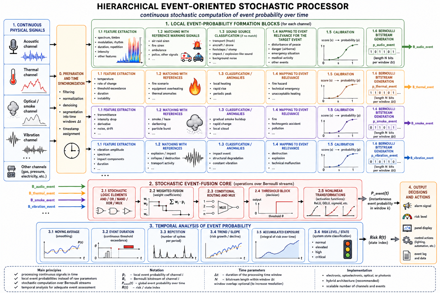
The proposed architecture is intended for continuous processing of heterogeneous physical signals whose relevance is defined not only by their instantaneous values, but also by their contribution to a target event over time. In contrast to a conventional feature-level processing pipeline, where each extracted physical feature may be independently encoded and processed, the proposed processor first forms compact local event probabilities and then processes them as stochastic streams. This design is motivated by the observation that the number of low-level features can grow rapidly when each physical channel is decomposed into amplitude, spectral, temporal, statistical, and contextual descriptors. Directly converting all of these features into Bernoulli bitstreams would increase the number of streams, synchronization paths, stochastic gates, and physical channels required for implementation.
The overall structure of the proposed hierarchical event-oriented stochastic processor is shown in Figure 1.
The proposed processor is therefore organized hierarchically. Its first level consists of local event-probability formation blocks. Each block receives a set of features from one physical channel or from a closely related group of physical measurements. The function of this block is not to preserve all low-level features as separate processor inputs, but to convert them into a compact set of event-level probabilistic descriptors. For example, an acoustic block may convert sound energy, temporal modulation, repetition, and similarity to warning-like patterns into probabilities such as , , and . Similarly, a thermal block could convert temperature, rate of change, threshold duration, and local fluctuations into a thermal event probability, while an optical or smoke-related block could convert transmittance loss, attenuation slope, and fluctuation level into a smoke-event probability.
The second level of the architecture is the stochastic event-fusion core. Local event probabilities are encoded as Bernoulli bitstreams and processed using stochastic logic and functional operations. Depending on the target application, the fusion core may implement OR-like accumulation, AND-like confirmation, weighted fusion, thresholding, majority-like decisions, multiplexer-based conditional routing, or nonlinear activation-like transformations. The exact operation is task-specific, but the computational representation remains stochastic: probabilities are processed through bitstreams rather than only as deterministic floating-point values.
The third level is the temporal event-analysis layer. The output of the stochastic fusion core is interpreted as a time-resolved global event-probability signal,
rather than as a single static output. This signal can then be analyzed in terms of persistence above a threshold, repeated event episodes, moving average, trend, accumulated exposure, and risk-state transitions. This temporal layer is essential for event-oriented monitoring, because two signals with the same instantaneous event probability may have different practical meanings depending on whether the event is isolated, repeated, or sustained over a long interval.
A high-level representation of the proposed architecture can be written as
where denotes the raw or preprocessed signal from physical channel , is the corresponding feature vector, is a compact vector of local event probabilities, and is the Bernoulli bitstream representation of these probabilities. The final output is obtained by stochastic fusion of the local event streams.
In this formulation, the architecture is universal at the structural level but task-specific at the mapping level. The same processing sequence can be applied to acoustic, thermal, optical, vibration, gas, or other sensing channels. However, the mapping from features to local event probabilities must be designed and calibrated for each target event and application domain. Therefore, the processor does not rely on a universal feature-to-probability formula. Instead, it provides a general stochastic processing framework into which task-specific local event-probability formation blocks can be inserted.
2.1. Local Event-Probability Formation
The local event-probability formation block is the first computational level of the proposed processor. It converts a set of physical or derived signal features into one or more local event probabilities. This block is introduced to avoid direct expansion of all low-level signal descriptors into separate stochastic streams. Its role is especially important for signals with rich internal structure, such as acoustic, vibration, or optical time series.
Let be a feature vector extracted from physical channel over a time window centered at time :
A direct stochastic mapping would encode each feature into a separate bitstream. This gives bitstreams for a single physical channel. In contrast, the proposed hierarchical mapping forms a smaller number of local event probabilities,
where each represents the relevance of the channel features to a specific local event descriptor. For an acoustic channel, these descriptors may correspond to a warning-like sound, acoustic disturbance, source confidence, or emergency-related sound activity. For a thermal channel, they may correspond to overheating, fast temperature rise, or abnormal thermal dynamics.
The mapping from to may be implemented using rule-based functions, calibrated logistic mappings, fuzzy logic, Bayesian models, small classifiers, lookup tables, or other task-specific models. The important point is that the output must be interpretable as an event probability or, at minimum, as an event score that can be calibrated into a probability. Therefore, it is useful to distinguish between an event score and an event probability . The score may be an arbitrary normalized detector output, while the probability should be calibrated so that its numerical value is meaningful for event-level processing.
A simple calibration relation can be expressed as
where is a sigmoid function, controls the sharpness of the transition, and is the event-score threshold. This formulation is not intended as the only possible calibration method. It is used here as a simple and transparent mapping for the numerical proof of principle.
2.2. Bernoulli Event-Bitstream Representation
After local event probabilities are formed, they are encoded into Bernoulli bitstreams. For a local event probability , a Bernoulli bitstream of length is defined as
where
The probability estimate obtained from this bitstream is
Thus, the bitstream represents the local event probability statistically. Increasing reduces the sampling variance of the estimate, but also increases the processing latency, memory requirements, and synchronization burden. Therefore, bitstream length is a key design parameter of the proposed processor.
In the context of continuous monitoring, a separate bitstream is generated for each processing window. If the monitoring interval is divided into time windows of duration , then the processor operates on a sequence of bitstream packets,
where is the number of time windows. This packet-based interpretation is useful for physical implementations because it explicitly separates the temporal monitoring scale from the bitstream length used within each window.
The bitstream representation also introduces an important source of uncertainty. Even if the local event probability is known exactly, its stochastic estimate fluctuates due to finite . This finite-bitstream uncertainty is not a defect of the model; it is an intrinsic part of stochastic computing and must be quantified when evaluating the processor output.
2.3. Stochastic Event-Fusion Core
The stochastic event-fusion core combines local Bernoulli event streams into a global event-probability estimate. The specific fusion rule depends on the semantics of the target event. If the event may be triggered by any of several local indicators, an OR-like stochastic fusion can be used. If several conditions must be simultaneously satisfied, an AND-like confirmation can be used. If the local indicators have different relevance levels, a weighted fusion can be used. If one local event selects between processing branches, a multiplexer-based conditional operation can be applied.
For example, if two independent local event streams and encode probabilities and , an AND operation estimates
while an OR operation estimates
A weighted event-fusion operation can be expressed at the probability level as
where are task-specific weights. In stochastic hardware, such a weighted operation may be approximated using multiplexer-based selection, stochastic averaging, or correlation-aware accumulation mechanisms.
The proposed architecture does not require a single universal fusion operation. Instead, it treats the stochastic event-fusion core as a configurable processing block. This is important because the meaning of a local event probability depends on the target application. For example, a warning-like acoustic event may be sufficient to increase a disturbance probability, while a fire-related event may require simultaneous support from smoke, thermal, and gas-related indicators. Therefore, fusion logic must be selected according to the physical and semantic structure of the monitored event.
2.4. Continuous Event-Probability Monitoring
A central feature of the proposed processor is that it operates cyclically over time. The output is not a single probability value but a time-resolved signal,
where denotes the processing window. This output can be interpreted as the global event probability estimated by the stochastic fusion core for the -th time window.
The temporal behavior of is often more informative than its instantaneous value. A short isolated peak, repeated peaks, and a prolonged elevated probability may have different meanings even if they reach similar maximum levels. Therefore, the processor output is further analyzed using temporal metrics such as moving average, persistence above threshold, number of event episodes, accumulated exposure, and trend.
For example, a moving average can be written as
where is the averaging window. Accumulated exposure is quantified in the numerical setup section.
These temporal descriptors allow the processor to distinguish between transient, repeated, and sustained event conditions. This is particularly important for monitoring applications where risk is not determined only by the instantaneous event probability, but also by duration, repetition rate, and temporal trend.
2.5. Direct Feature Mapping versus Hierarchical Event Mapping
The proposed hierarchy introduces a deliberate compression step. This compression is beneficial because it reduces the number of stochastic streams and simplifies the architecture. However, it may also introduce modeling error because multiple low-level features are replaced by fewer local event probabilities. Therefore, the proposed approach should be evaluated not only by output accuracy, but also by the trade-off between stream reduction, interpretability, and probability-estimation error.
In the direct mapping strategy, each feature is converted into a separate Bernoulli stream:
If the channel has features, it produces streams. In the hierarchical event mapping strategy, the same features are first compressed into local event probabilities:
This reduces the number of streams, but the output may deviate from the direct feature-level representation. In this work, the acoustic demonstration explicitly compares these two strategies to quantify the compression–accuracy trade-off.
The purpose of this comparison is not to show that hierarchical event mapping always produces lower numerical error. Rather, the purpose is to demonstrate that event-level representation can reduce the architectural burden while preserving the main event-related temporal structure. This distinction is important because the proposed processor is intended for event monitoring, where continuous interpretability and scalable stream management are as important as instantaneous reconstruction accuracy.
3. Acoustic Proof-of-Principle Model
The proposed architecture is demonstrated using a synthetic acoustic monitoring scenario. The acoustic channel is selected as an illustrative example because sound signals naturally contain multiple low-level descriptors, including amplitude, spectral structure, modulation, repetition, duration, and source-related characteristics. At the same time, many monitoring tasks do not require all of these descriptors as independent processor inputs. Instead, the relevant quantity is often the contribution of the acoustic channel to a target event, such as warning-like acoustic activity, acoustic disturbance, or emergency-related sound occurrence.
The goal of this proof-of-principle model is not to develop a complete acoustic event detection system. Such systems have been extensively studied in the literature, including acoustic scene classification, sound event detection, siren detection, emergency vehicle sound recognition, and urban sound monitoring [75,76,77,78,79,80,81,82,83,84,85,86,87,88,89,90,91,92]. Here, the acoustic signal is used to demonstrate the proposed processor pathway from low-level physical features to local event probabilities, then to Bernoulli event streams, and finally to a time-resolved global event-probability output.
The numerical experiment is based on synthetic acoustic-event scenarios. This allows full control of the event timeline, signal features, local probability mappings, and stochastic bitstream parameters. The model is therefore intended as an architecture-level proof of principle rather than as a benchmark on real-world acoustic datasets.
3.1. Time-Windowed Monitoring Scenario
The monitoring interval is divided into discrete time windows of duration . In the numerical demonstration, a 30-minute monitoring sequence is used, with a processing window of 5 s. This gives processing windows. Each window is assigned one of the following scenario labels: background, isolated warning, repeated warning, vehicle/aircraft hum, impact-like, and prolonged warning.
The synthetic timeline contains both short and sustained events. The background scenario represents normal acoustic conditions. The isolated-warning scenario represents a short warning-like event. The repeated-warning scenario represents multiple warning-like patterns appearing over a longer interval. The vehicle/aircraft-hum scenario represents a lower-frequency sustained acoustic source. The impact-like scenario represents a short high-energy transient. The prolonged-warning scenario represents a sustained high-probability warning-like state.
This scenario design is intentionally simple. It is not intended to reproduce the full diversity of real urban acoustics. Instead, it provides controlled event types with different temporal structures, allowing the processor to be evaluated on isolated, repeated, transient, and prolonged acoustic events.
3.2. Acoustic Feature Representation
For each time window , the acoustic channel is represented by a compact feature vector,
In the proof-of-principle simulation, the features are normalized to the interval [0,1] and are designed to represent event-relevant acoustic descriptors rather than raw waveform samples. The model uses features such as:
where e[k] denotes acoustic energy or intensity, s[k] denotes similarity to a warning-like reference pattern, m[k] denotes temporal modulation or periodicity, r[k] denotes repetition strength, h[k] denotes low-frequency hum content, and q[k] denotes impact-like transient strength.
These features are not treated as final stochastic processor inputs. Instead, they are used inside the local acoustic event-probability formation block. This is a central distinction of the proposed architecture. The processor does not directly require separate Bernoulli streams for all low-level acoustic descriptors. Rather, these descriptors are first mapped into event-level quantities.
3.3. Local Acoustic Event-Probability Formation
The acoustic proof-of-principle block used in this study is summarized in Figure 2.
The local acoustic block converts the feature vector into a compact set of event probabilities. In the present demonstration, three local probabilities are formed: .
The first quantity, , represents the probability that the acoustic window contains a warning-like event. It depends mainly on the similarity to reference warning patterns, temporal modulation, and repetition. The second quantity, , represents the probability that the acoustic channel indicates a disturbance or abnormal acoustic activity. It may be influenced by warning-like patterns, impact-like events, and sustained low-frequency hum. The third quantity, , represents the confidence of the local acoustic interpretation. It is introduced to account for uncertainty in the local event-probability formation process.
The mapping can be written generally as
where
The function is task-specific. In a real acoustic monitoring system, it could be implemented using a trained classifier, a reference-pattern matching algorithm, a Bayesian detector, a rule-based model, or a hybrid signal-processing and machine-learning pipeline. In the present proof-of-principle model, a transparent rule-based score followed by sigmoid calibration is used. This choice makes the numerical experiment reproducible and interpretable.
The event-score-to-probability mapping has the form
where is an intermediate event score, is a threshold, is a slope parameter, and
is the sigmoid function. This calibration step distinguishes an arbitrary detector score from a probability-like event descriptor.
3.4. Reference Matching and Source-Level Interpretation
A key motivation for the acoustic example is that low-level acoustic parameters are not sufficient to define the event-level meaning of a sound. A warning signal may appear with different tones, intensities, durations, or recording conditions, yet still belong to the same semantic event class. Conversely, sounds with similar energy or dominant frequency may have different meanings depending on their source.
Therefore, the acoustic local block is conceptually organized around source-level and event-level interpretation. The first stage evaluates similarity to reference warning-like patterns. The second stage estimates whether the sound belongs to a disturbance or abnormal activity class. The third stage assigns a confidence level to the local acoustic interpretation.
In a practical system, reference matching could be performed using templates, spectral-temporal similarity measures, log-mel or MFCC-based descriptors, neural embeddings, or acoustic-event classifiers. The present model does not attempt to optimize this stage. Instead, it abstracts the reference-matching result as a normalized feature that contributes to . This abstraction is sufficient for demonstrating how a local acoustic interpretation can be converted into a stochastic event stream.
3.5. Local Bernoulli Event Streams
After local event probabilities are obtained, each probability is encoded as a Bernoulli bitstream. For the acoustic block, the resulting streams are
For a bitstream length , each stream is defined as
with
where denotes warning, disturbance, or confidence.
The stochastic estimate of the corresponding probability is
In the baseline simulation, is used as the main bitstream length. Additional values of are tested to evaluate sensitivity to bitstream length. This analysis is necessary because a shorter bitstream reduces computational latency and hardware burden, while a longer bitstream improves statistical accuracy.
3.6. Acoustic Event-Fusion Output
The local acoustic streams are combined to produce a global event-probability estimate for each time window. In the demonstration, the fusion operation is intentionally simple and interpretable. It combines warning-like evidence, disturbance evidence, and confidence information into a time-resolved event probability,
At the probability level, the fusion can be represented generically as
where is the selected event-fusion rule. At the stochastic level, the corresponding operation is performed on the Bernoulli streams,
The output event probability is estimated as
This output is then analyzed over time. The central result of the demonstration is therefore not only whether an acoustic event is detected in a particular window, but how evolves across the full monitoring interval.
3.7. Direct versus Hierarchical Acoustic Mapping
The acoustic example is also used to compare direct feature-to-bitstream mapping with the proposed hierarchical event-probability mapping.
In the direct approach, each acoustic feature is independently encoded as a stochastic stream:
This gives six stochastic streams for the acoustic channel in the present model. In a more realistic acoustic system, the number of features could be much larger because spectral, temporal, cepstral, and neural-embedding descriptors may all be included.
In the hierarchical approach, these features are first mapped to three local event probabilities:
Only these event-level probabilities are encoded as stochastic streams. Thus, in the present demonstration, the number of streams is reduced from six to three. This reduction is modest but sufficient to illustrate the architectural principle. In higher-dimensional physical channels, the same mechanism can provide a stronger reduction.
The comparison between the direct and hierarchical strategies is used to quantify the compression–accuracy trade-off. Direct mapping preserves more low-level information and may produce lower numerical error in certain cases. Hierarchical mapping reduces the number of streams and improves event-level interpretability, but may introduce additional modeling error due to feature compression. Both effects are evaluated in the numerical results.
4. Numerical Experiment Setup
The numerical experiment was designed as a reproducible architecture-level proof of principle. Its purpose is not to benchmark a real acoustic event detection system, but to demonstrate the complete processing pathway of the proposed hierarchical event-oriented stochastic processor. The simulation starts from a time-windowed acoustic scenario, generates normalized acoustic features, forms local event probabilities, converts them into Bernoulli bitstreams, performs stochastic event fusion, and finally analyzes the time-resolved output .
All calculations were implemented in a Python/Colab notebook. The notebook was structured to automatically generate the figures and tables used in the paper and supplementary material. Figures were exported at 600 dpi to ensure publication-quality resolution.
4.1. Monitoring Timeline and Scenario Labels
The simulated monitoring interval corresponds to 30 min of continuous observation. The signal is divided into processing windows of duration Δt=5 s. This gives K=360 time windows. The time axis is represented in minutes as
Each processing window is assigned one acoustic scenario label. The baseline condition is background acoustic activity. Several event intervals are then inserted into the 30 min timeline to represent different temporal structures of acoustic events.
The simulated scenarios are summarized in Table 2.
This timeline allows the model to test several distinct temporal behaviors: isolated events, repeated events, prolonged events, sustained non-warning acoustic activity, and short impulsive disturbances.
4.2. Synthetic Acoustic Feature Generation
For each time window, a normalized acoustic feature vector is generated:
where: e[k] is the acoustic energy or intensity feature; s[k] is similarity to a warning-like acoustic pattern; m[k] is temporal modulation or periodicity; r[k] is repetition strength; h[k] is low-frequency hum content; q[k] is impact-like transient strength.
All features are normalized to the interval [0,1]. The feature values are generated synthetically according to the assigned scenario label. Background windows have low event-related features. Warning-like scenarios have high warning similarity, modulation, and repetition features. Vehicle- or aircraft-like hum has increased low-frequency hum and moderate disturbance-related features. Impact-like events have high transient strength but limited persistence.
The synthetic generation approach was selected to provide full control over the event structure and to make the numerical demonstration transparent and reproducible. The model is therefore not intended to replace real acoustic feature extraction from waveform or spectrogram data.
4.3. Local Event-Probability Formation
The synthetic acoustic features are converted into three local event probabilities:
The warning probability represents the local probability of a warning-like acoustic event. It is mainly controlled by warning similarity, temporal modulation, and repetition. The disturbance probability represents the local probability of an acoustically relevant disturbance and is influenced by warning-like activity, impact-like events, and sustained hum. The confidence probability represents the reliability of the local interpretation of the acoustic signal.
Intermediate event scores are first formed from weighted combinations of acoustic features. These scores are then converted into probability-like outputs using a sigmoid calibration function,
where is the event score, is the threshold parameter, and controls the slope of the score-to-probability transition.
This calibration step is included to emphasize the distinction between arbitrary feature scores and event probabilities. In this proof-of-principle model, the calibration is rule-based and synthetic. In a real application, it could be replaced by empirical calibration, logistic regression, Bayesian calibration, isotonic regression, or a trained classifier output calibration.
4.4. Bernoulli Bitstream Generation
Each local event probability is represented by a Bernoulli bitstream. For a probability , where denotes warning, disturbance, or confidence, a bitstream of length is generated as
with
The corresponding stochastic estimate is
The baseline simulation uses .
To evaluate the effect of bitstream length on statistical error, additional values were tested:
This analysis is important because bitstream length directly affects the trade-off between statistical accuracy and processing cost. Shorter bitstreams reduce latency and hardware burden but increase stochastic sampling error. Longer bitstreams improve probability estimation but require more processing time and synchronization.
For a stochastic fusion operation to be meaningful, all event streams entering the fusion core must refer to the same processing window and must be represented by compatible bitstream packets. Therefore, the architecture assumes a preparation and time-synchronization stage that aligns local event probabilities by timestamp, buffers delayed channels, and generates bitstreams of a common length N for each window. Without this alignment, stochastic logic operations could combine event evidence originating from different physical time intervals, leading to incorrect event interpretation.
4.5. Stochastic Event-Fusion Rules
The local Bernoulli event streams are processed by a stochastic event-fusion core. The proof-of-principle model includes several simple fusion operations designed to illustrate different semantic roles of local event probabilities.
First, an AND-like confirmation operation combines warning-like evidence with confidence:
At the probability level, assuming statistical independence, this approximates
Second, an OR-like accumulation operation combines warning-related and disturbance-related evidence:
At the probability level, for independent streams, this approximates
Third, a weighted fusion output is calculated to obtain the final time-resolved event probability. In the numerical demonstration, the global event probability is formed as a weighted combination of local event estimates and stochastic fusion outputs. This represents a configurable event-fusion rule rather than a universal formula.
The resulting processor output is denoted as .
This value is computed for each time window, producing a time-resolved event-probability signal.
4.6. Temporal Analysis Metrics
The output is analyzed as a continuous monitoring signal. Several temporal metrics are calculated.
The moving average is computed as
where is the number of windows in the averaging interval. In the baseline analysis, a 1 min moving average is used.
Persistence above threshold is calculated as the total duration for which the event probability exceeds a selected threshold:
where is the event threshold and is the indicator function.
Accumulated exposure is defined as
This quantity reflects the cumulative event load over the monitoring interval. It is useful for distinguishing a single short peak from repeated or prolonged elevated event probability.
The number of event episodes is estimated by counting contiguous intervals in which exceeds the event threshold. This metric differentiates isolated events from repeated event activity.
4.7. Direct Feature-to-Bitstream Mapping Baseline
To evaluate the benefit and cost of hierarchical event mapping, a direct feature-to-bitstream baseline is included. In the direct approach, each acoustic feature is independently converted into a Bernoulli bitstream:
Thus, the direct acoustic representation uses six bitstreams in the present model. In contrast, the hierarchical representation uses three event-level bitstreams:
The stream reduction factor is therefore
Although this reduction is moderate in the present simplified acoustic example, it demonstrates the architectural mechanism. In realistic acoustic monitoring systems, the number of low-level features can be much larger, making event-level compression more significant.
The direct and hierarchical strategies are compared using probability-estimation error and stream count. The comparison is not intended to prove that hierarchical mapping is always more accurate. Rather, it evaluates whether the hierarchical strategy can reduce the number of stochastic streams while preserving the main temporal event structure.
4.8. Evaluation Metrics and Outputs
The following metrics are computed in the numerical experiment:
- Mean event probability by scenario. The average value of is computed for each scenario label.
- Local bitstream reconstruction error. The RMSE between each local probability and its stochastic estimate is calculated.
- Bitstream-length sensitivity. The effect of on stochastic estimation error is evaluated for
- Temporal monitoring metrics. Persistence above threshold, number of event episodes, moving average, and accumulated exposure are computed from .
- Direct versus hierarchical mapping error. The direct feature-to-bitstream mapping and the hierarchical event-probability mapping are compared in terms of stream count and RMSE.
The simulation automatically generates publication-quality figures and tables. The main outputs include: synthetic acoustic feature timelines; local event-probability curves; Bernoulli bitstream reconstruction plots; stochastic event-fusion output; time-resolved ; temporal monitoring metrics; direct versus hierarchical mapping comparison; bitstream-length sensitivity plots and tables. These outputs provide the basis for the numerical results presented in the next section.
5. Results
The numerical experiment demonstrates the complete processing pathway of the proposed hierarchical event-oriented stochastic processor. The results are presented in six steps: generation of acoustic-event scenarios, formation of local event probabilities, Bernoulli bitstream reconstruction, stochastic event fusion, temporal event-probability monitoring, and comparison between direct and hierarchical stochastic mappings.
5.1. Synthetic Acoustic Scenarios and Feature-Level Response
The 30 min monitoring sequence contains background activity and five inserted acoustic-event scenarios: isolated warning, repeated warning, vehicle- or aircraft-like hum, impact-like disturbance, and prolonged warning. These scenarios were selected to represent different temporal event structures rather than to reproduce real acoustic recordings. The purpose was to test whether the proposed processor can distinguish transient, repeated, sustained, and non-warning acoustic activity at the event-probability level.
The generated feature trajectories for the synthetic acoustic monitoring sequence are shown in Figure 3.
The generated feature trajectories show that the warning-like scenarios produce high values of warning similarity, temporal modulation, and repetition-related features. The vehicle- or aircraft-like scenario mainly increases the low-frequency hum descriptor, while the impact-like scenario produces a short increase in the transient-impact feature. Background intervals remain at low event-related feature levels. Thus, the synthetic features provide a controlled input for evaluating local event-probability formation.
This feature-level behavior confirms that the scenario generator produces distinguishable acoustic patterns suitable for testing the proposed architecture. However, the features themselves are not used as final processor-level inputs in the hierarchical approach. Instead, they are converted into local event probabilities.
5.2. Local Acoustic Event Probabilities
The local acoustic block converts the six normalized acoustic features into three event-level probabilities: .
The warning probability increases strongly during isolated, repeated, and prolonged warning-like intervals. The disturbance probability responds not only to warning-like acoustic patterns but also to impact-like and sustained hum-like conditions. The confidence probability remains higher when the local acoustic interpretation is consistent and lower when the feature combination is less specific.
This confirms the intended role of the local event-probability formation block: it compresses several low-level acoustic descriptors into a compact set of event-level quantities. Instead of sending all acoustic features directly to the stochastic fusion core, the processor receives local event probabilities that already carry task-relevant semantic meaning.
The resulting local acoustic event probabilities are presented in Figure 4.
The resulting local probabilities are therefore better suited for event-oriented stochastic processing than raw feature streams. They represent not merely “frequency,” “energy,” or “modulation,” but event-level acoustic evidence.
5.3. Bernoulli Bitstream Reconstruction Accuracy
Each local event probability was encoded as a Bernoulli bitstream. The baseline bitstream length was .
The stochastic estimate of each probability was obtained as the fraction of ones in the generated bitstream. The RMSE between the ideal local probability and the stochastic estimate was calculated for each local event stream.
Examples of Bernoulli event-bitstream realizations are shown in Figure 5.

Table 3.
Local Bernoulli bitstream reconstruction error for
| Local probability | RMSE |
| pwarning(t) | 0.0185 |
| pdisturbance(t) | 0.0262 |
| pconfidence(t) | 0.0248 |
The reconstruction errors are small for the baseline stream length, indicating that provides a sufficiently stable stochastic representation for the proof-of-principle demonstration. As expected for Bernoulli sampling, the stochastic estimate fluctuates around the ideal probability, and the magnitude of the fluctuation depends on bitstream length and probability value.
These results confirm that the local event probabilities can be represented by finite Bernoulli bitstreams with controlled statistical error. This is important because the subsequent event-fusion core operates on stochastic streams rather than directly on floating-point probabilities.
5.4. Stochastic Event Fusion and Time-Resolved Output
The local event streams were combined by the stochastic event-fusion core. The resulting output is a time-resolved global event-probability signal,
The mean values of computed for each scenario are summarized in Table 4.
The background scenario produces a low mean event probability. Warning-like scenarios produce high values, with repeated and prolonged warning intervals reaching mean probabilities above 0.90. The isolated warning scenario also produces a high mean value, but only over a short interval. The vehicle- or aircraft-like hum and impact-like scenarios produce intermediate values, reflecting their disturbance-related but less warning-specific character.
The stochastic fusion output and the resulting time-resolved event probability are shown in Figure 6.
These results show that the processor output is sensitive to the event-level meaning of the acoustic pattern. It does not simply respond to any acoustic activity as a high-probability event. Instead, warning-like repeated and prolonged patterns produce stronger event probabilities than background, hum-like, or impact-like scenarios.
5.5. Temporal Event-Probability Monitoring
A central goal of the proposed architecture is continuous monitoring rather than one-time classification. Therefore, the most important output is the full time series , not only the mean value for each scenario.
The time-resolved output shows low event probability during background intervals, a short peak during the isolated-warning event, repeated high-probability intervals during repeated-warning activity, a moderate response during the vehicle- or aircraft-like hum interval, a short transient response during the impact-like interval, and sustained high probability during the prolonged-warning interval.
Temporal analysis of the time-resolved event-probability signal is presented in Figure 7.
Temporal analysis was performed using a threshold-based persistence metric, moving average, accumulated exposure, and event-episode counting. The baseline temporal metrics are summarized in Table 5.
The persistence above threshold indicates that the processor output remains in an elevated event-probability state for a total of 9.42 min during the 30 min monitoring sequence. The number of event episodes equals 3, corresponding to temporally separated high-probability event regions. The accumulated exposure value reflects the integrated event-probability load over the full monitoring interval.
These temporal metrics demonstrate why continuous monitoring is important. A short isolated warning, repeated warnings, and prolonged warning activity may all produce high instantaneous event probabilities, but their temporal signatures are different. The proposed processor therefore supports not only event detection but also event-state interpretation over time.
The accumulated event exposure derived from is shown in Figure 8.
5.6. Direct Feature-to-Bitstream Mapping versus Hierarchical Event Mapping
The direct feature-to-bitstream baseline encodes each of the six acoustic features as an independent stochastic stream. The hierarchical mapping compresses these features into three local event probabilities and then encodes only those event probabilities as Bernoulli streams. Thus, in the present demonstration, the number of streams is reduced from six to three: .
The stream-count reduction achieved by hierarchical event mapping is illustrated in Figure 9.
To evaluate the effect of this compression, the direct and hierarchical mappings were compared over several bitstream lengths. The resulting RMSE values are shown in Table 6.
The direct mapping produces lower RMSE for all tested bitstream lengths. This is expected because direct mapping preserves more feature-level information and avoids the additional modeling error introduced by event-level compression. In contrast, the hierarchical mapping reduces the number of streams but introduces a compression error associated with mapping several low-level features into fewer local event probabilities.
This result is important because it shows that hierarchical event mapping should not be interpreted as a universally more accurate numerical representation. Its advantage is architectural rather than purely numerical: it reduces the number of stochastic streams, improves event-level interpretability, and makes the processor more scalable for continuous monitoring.
Thus, the proposed architecture introduces a compression–accuracy trade-off. Direct mapping may be preferable when preserving all feature-level details is critical and the number of streams is manageable. Hierarchical event mapping becomes more attractive when the number of physical features is large, when synchronization and hardware complexity are limiting factors, or when event-level interpretation is more important than exact feature-level reconstruction.
5.7. Effect of Bitstream Length
The results also confirm the expected influence of bitstream length. In the direct mapping case, the RMSE decreases as the bitstream length increases from to . This reflects the reduction of Bernoulli sampling error with longer streams.
For the hierarchical mapping, the RMSE decreases only slightly and remains around 0.09. This indicates that, in the current model, the hierarchical error is dominated not by Bernoulli sampling noise but by the event-level compression model. Increasing the bitstream length cannot remove this modeling error. This distinction is important for processor design: once stochastic sampling error becomes sufficiently small, further improvements require better event-probability formation rather than longer bitstreams.
The effect of bitstream length on the direct and hierarchical mappings is summarized in Figure 10.
Therefore, the bitstream-length analysis separates two sources of error:
- Stochastic sampling error, which decreases with increasing ;
- Event-compression error, which depends on the local event-probability formation model.
This distinction should be considered when optimizing future implementations.
5.8. Summary of Numerical Findings
The numerical proof of principle supports the main architectural claims of the proposed processor.
First, the acoustic local block successfully converts low-level features into compact local event probabilities. This demonstrates the feasibility of replacing direct feature-level stochastic encoding with event-level encoding.
Second, Bernoulli bitstreams of length reproduce the local event probabilities with low reconstruction error. This confirms that local event probabilities can be represented in stochastic form with controlled statistical fluctuations.
Third, stochastic event fusion produces a time-resolved global probability signal . This output distinguishes background, isolated warning, repeated warning, prolonged warning, hum-like, and impact-like acoustic scenarios.
Fourth, temporal metrics such as persistence, number of event episodes, moving average, and accumulated exposure provide information that is not available from a single static probability value. This supports the idea that the processor should be interpreted as a continuous monitoring system.
Fifth, the direct versus hierarchical comparison demonstrates a clear compression–accuracy trade-off. Hierarchical event mapping reduces the number of bitstreams from six to three in the present example, but produces higher RMSE than direct feature mapping. This result is consistent with the intended role of the hierarchy: it improves architectural compactness and event-level interpretability, not necessarily raw numerical reconstruction accuracy.
Overall, the results validate the proposed architecture as an event-oriented stochastic processing framework. The acoustic demonstration shows how physical signal features can be converted into local event probabilities, encoded as Bernoulli streams, stochastically fused, and analyzed as a time-resolved event-probability output.
6. Discussion
The numerical proof of principle demonstrates the feasibility of representing event-oriented physical information as compact Bernoulli event streams and processing these streams in a continuous stochastic monitoring architecture. The results should be interpreted at the architectural level rather than as a benchmark of acoustic event detection accuracy. The main contribution is the proposed processing principle: local event-probability formation, stochastic event fusion, and time-resolved global event-probability monitoring.
6.1. Interpretation of the Hierarchical Event-Probability Approach
The proposed architecture changes the role of low-level physical features in stochastic processing. In a direct feature-to-bitstream approach, each signal descriptor is treated as a separate stochastic input. This is straightforward, but it scales poorly when the number of descriptors grows. Acoustic signals provide a clear example: amplitude, dominant frequency, spectral structure, modulation, repetition, duration, transient strength, and source-class indicators can all be useful, but encoding each as a separate Bernoulli stream would rapidly increase stream count and synchronization complexity.
The hierarchical approach addresses this issue by introducing local event-probability formation blocks. These blocks do not discard the low-level features; instead, they use them internally to estimate event-level descriptors. In the acoustic example, the feature vector is compressed into warning, disturbance, and confidence probabilities. These probabilities are more directly aligned with the target monitoring task than the original low-level features.
Therefore, the architecture does not simply perform dimensionality reduction. It performs event-oriented abstraction. The output of the local block is not an arbitrary compressed feature vector but a compact probabilistic representation of event relevance. This makes the subsequent stochastic processing stage more interpretable, because the stochastic streams represent event-level quantities rather than raw physical descriptors.
6.2. Compression–Accuracy Trade-Off
The direct versus hierarchical comparison shows that the hierarchical representation introduces a compression–accuracy trade-off. In the present demonstration, direct feature-to-bitstream mapping gives lower RMSE than hierarchical mapping for all tested bitstream lengths. This result is expected because direct mapping preserves the original feature-level information, whereas hierarchical mapping compresses six acoustic features into three event probabilities.
This observation is important for the correct interpretation of the proposed architecture. The hierarchical approach should not be presented as a universal method for reducing numerical error. Its primary advantage is architectural compactness and semantic interpretability. By reducing the number of streams, the architecture reduces the burden on stream generation, synchronization, routing, and stochastic fusion. These factors are especially important for optical, photonic, or hybrid implementations where each additional stream may correspond to an additional physical channel, optical path, detector, modulator, or processing element.
The results also show that increasing bitstream length does not remove the main error source in the hierarchical case. For the direct mapping, RMSE decreases with increasing , indicating that Bernoulli sampling noise is a dominant contribution. For the hierarchical mapping, RMSE remains close to 0.09 even for longer streams, indicating that the error is mainly caused by event-level compression. This separation is useful for future design: bitstream length should be increased only until stochastic sampling error becomes acceptable; further improvement then requires better local event-probability formation rather than longer streams.
6.3. Importance of Continuous Monitoring
A key aspect of the proposed processor is that its output is a time-resolved probability signal, , rather than a single static decision. This is essential for event-oriented monitoring tasks. A short isolated event, repeated events, and a prolonged high-probability state can all produce high instantaneous probability values, but they have different temporal meanings.
The numerical results illustrate this distinction. The isolated warning scenario produces a short high-probability response. The repeated-warning scenario produces multiple elevated intervals. The prolonged-warning scenario produces a sustained high-probability state. These cases are not equivalent from the point of view of monitoring, risk assessment, or decision support. Temporal descriptors such as persistence above threshold, accumulated exposure, and event-episode count provide information that cannot be captured by a single probability value.
This continuous-processing interpretation also strengthens the stochastic nature of the proposed architecture. The processor is not merely a one-time classifier followed by stochastic encoding. Instead, it repeatedly forms local event probabilities, generates Bernoulli event streams, fuses them, and updates over time. The object of computation is therefore a stochastic event-probability process.
6.4. Relation to Optical and Photonic Stochastic Processors
The present work is formulated at the architecture and numerical proof-of-principle level. Nevertheless, it is motivated by optical and photonic stochastic computing. Existing optical SC and probabilistic photonic works demonstrate that stochastic logic, optical random sources, photonic probabilistic bits, stochastic neural components, and optical accelerators are physically plausible building blocks for future processors [21,22,23,24,25,26,27,28,29,30,31,32,33,34,35,36,37,38,39,40]. Optical logic gates and photonic combinational circuits also provide a basis for implementing higher-level processing blocks [41,42,43,44,45,46,47,48,49,50,51,52,53,54].
The proposed architecture can be interpreted as a processor-level framework that could organize such building blocks for event-oriented monitoring. Local event probabilities may initially be formed in digital, electronic, or optoelectronic subsystems. These probabilities can then be encoded into optical or photonic stochastic streams for fusion. Alternatively, in a more advanced implementation, some local event-probability formation and fusion functions could themselves be implemented optically or photonically.
For a bulk-optics demonstrator, the architecture is also useful because it separates the conceptual processor levels. Local event probabilities can be generated electronically or computationally, while the stochastic fusion core can be demonstrated using optical logic modules. This hybrid pathway is realistic for early experimental validation. A fully integrated photonic implementation would require additional development of compact random-bit generation, optical stream synchronization, correlation control, and scalable routing.
Thus, the proposed architecture should not be interpreted as a claim that all processing stages must already be fully optical. Rather, it defines a hierarchical processing framework that is compatible with electronic, optical, photonic, and hybrid implementations.
6.5. Local Event Blocks versus External Frontend
A possible criticism is that the local event-probability formation block may appear to be an external intelligent frontend rather than part of the stochastic processor. In this work, the local blocks are treated as the first computational level of the processor architecture. Their purpose is to transform physical-channel features into local event probabilities that can be processed stochastically.
This distinction is important. If the local block produced a final decision, the stochastic processor would indeed become unnecessary. However, in the proposed architecture, local blocks do not determine the final global event state. They produce intermediate event-probability streams. The final output is obtained only after stochastic fusion and temporal analysis.
For example, an acoustic block may estimate , and . These quantities may be useful, but they are not yet the final target event probability. In a multisensor version of the processor, they would be fused with thermal, optical, vibration, gas, or contextual event streams. Therefore, local event-probability formation is not a replacement for the stochastic processor; it is the first level of its hierarchy.
6.6. Limitations of the Current Proof-of-Principle Model
The present study has several limitations. First, the acoustic scenario is synthetic. The generated features are designed to represent idealized warning-like, disturbance-like, hum-like, impact-like, and background patterns. The model does not yet use real acoustic recordings, measured urban soundscapes, or benchmark datasets. Second, the local event-probability formation model is rule-based. It uses transparent feature combinations and sigmoid calibration for interpretability. In practical applications, this block would need to be trained, calibrated, and validated on real data.
Third, only one physical channel is modeled in detail. The architecture is intended to support multiple physical channels, but the present preprint demonstrates the concept using the acoustic channel only. Multisensor demonstrations involving thermal, optical/smoke, vibration, gas, or context channels are left for future work. Fourth, the stochastic fusion rules are simple. The proof of principle uses interpretable AND-like, OR-like, and weighted fusion operations. More complex event-fusion logic could include adaptive weights, correlation-aware fusion, Bayesian fusion, stochastic finite-state machines, or learned stochastic decision structures. Fifth, correlation between streams is not fully explored. In stochastic computing, correlation may be harmful or beneficial depending on the operation. The present model uses the standard Bernoulli-stream assumption for the baseline demonstration. Future work should explicitly analyze correlation control, decorrelation, and intentional correlation in event-fusion operations. Sixth, the model does not claim hardware superiority over digital processing. The numerical demonstration is not an energy or latency benchmark. Its purpose is to establish the architectural concept and show the processing pathway from physical features to time-resolved stochastic event probability.
6.7. Future Extensions
The next step is to extend the proof of principle from a single acoustic channel to a multisensor event-oriented processor. In such a model, each physical channel would have its own local event-probability formation block. For example:
could be encoded as Bernoulli event streams and fused into a global event probability.
Another important direction is to test the architecture on real or semi-real data. For the acoustic case, this could involve urban sound datasets, siren-detection datasets, or controlled recordings. For optical or environmental monitoring, measured smoke-transmittance, thermal, vibration, or gas-sensor data could be used.
The architecture should also be evaluated under degraded conditions, including missing channels, stale data, asynchronous sampling, noisy features, and conflicting local event probabilities. These conditions are important for continuous monitoring systems and would make the event-oriented stochastic processor more realistic.
Finally, future work should examine hardware implementation pathways. The proposed architecture can support digital, electronic, bulk-optics, integrated photonic, and hybrid realizations. Early experimental work may use bulk-optical stochastic logic modules for fusion while retaining digital local event-probability formation. Later implementations may replace more of the hierarchy with optical or photonic processing blocks.
6.8. Implications for Event-Oriented Stochastic Processing
The proposed architecture suggests that stochastic computing can be extended beyond isolated arithmetic blocks and neural-network accelerators toward continuous event-probability monitoring. This requires a shift from feature-level stochastic representation to event-level stochastic representation.
The main implication is that stochastic processors should not necessarily receive all physical features as independent streams. Instead, local event-probability formation can reduce the stream count and provide more meaningful processor inputs. The stochastic processor then operates on event probabilities rather than raw physical descriptors.
This interpretation is especially relevant for sensing systems, where uncertainty, noise, incomplete data, and time-dependent event evolution are natural. In such systems, the goal is often not to compute a precise deterministic value, but to continuously update the probability of a target event and support decisions based on its temporal behavior.
7. Conclusion
This work proposed a hierarchical event-oriented stochastic processor architecture for continuous monitoring of event probabilities. The main motivation was the scalability limitation of direct feature-to-bitstream mapping. When physical signals are decomposed into many low-level descriptors, direct encoding of each descriptor as an independent Bernoulli bitstream rapidly increases the number of streams, synchronization paths, stochastic processing blocks, and physical channels required for implementation.
The proposed architecture addresses this problem by introducing local event-probability formation blocks. These blocks convert task-relevant physical features into compact local event probabilities before stochastic encoding. The local probabilities are then represented as Bernoulli bitstreams and processed by a stochastic event-fusion core. The processor output is not a single static value, but a time-resolved global event-probability signal, , which enables continuous monitoring of event persistence, repetition, temporal trend, and accumulated exposure.
A synthetic acoustic monitoring scenario was used as an architecture-level proof of principle. The acoustic example demonstrated the full processing pathway from low-level acoustic descriptors to local event probabilities, Bernoulli event streams, stochastic fusion, and time-resolved event-probability monitoring. The results showed that warning-like acoustic patterns produced high event probabilities, background intervals remained at low probability levels, and transient, repeated, and prolonged events could be distinguished through temporal analysis of .
The numerical results also demonstrated a clear compression–accuracy trade-off. Direct feature-to-bitstream mapping provided lower RMSE because it preserved more feature-level information. In contrast, hierarchical event mapping reduced the number of stochastic streams and improved event-level interpretability, but introduced additional compression error. This result supports the main architectural interpretation of the proposed approach: hierarchical event mapping should not be viewed as a universal accuracy-improvement method, but as a strategy for scalable, interpretable, event-level stochastic processing.
The proposed framework is compatible with digital, electronic, optical, photonic, and hybrid implementations. In early experimental systems, local event probabilities may be formed digitally or electronically, while stochastic fusion can be implemented using electronic, bulk-optical, or photonic logic modules. In future integrated implementations, a larger part of the hierarchy may be realized using optical or photonic stochastic computing elements.
Future work should extend the present acoustic proof of principle to multisensor scenarios involving thermal, optical, vibration, gas, and contextual channels. Further studies should also include real or semi-real datasets, calibrated local event-probability formation, explicit stream-correlation analysis, asynchronous sampling, missing or stale data, and experimental validation of optical or hybrid stochastic fusion modules. These extensions would allow the proposed architecture to evolve from a conceptual and numerical proof of principle toward a practical event-oriented stochastic processing platform for probabilistic sensing and decision-support systems.
Supplementary Materials
The following supporting information can be downloaded at the website of this paper posted on Preprints.org.
Data and Code Availability
The Python scripts, processed numerical outputs, and figure data used in the illustrative experiment are provided as supplementary material to this preprint.
Conflicts of Interest
The authors declare no conflict of interest.
References
- Lee YY, Abdul Halim Z. 2020. Stochastic computing in convolutional neural network implementation: a review. PeerJ Computer Science 6:e309. [CrossRef]
- Kim, J., Lim, K., & Kim, Y. (2026). Hardware-efficient stochastic computing-based neural networks with SNN-isomorphic LIF activation. Electronics, 15(4), 768. [CrossRef]
- Lunglmayr, M., Wiesinger, D., & Haselmayr, W. (2020). Design and analysis of efficient maximum/minimum circuits for stochastic computing. IEEE Transactions on Computers, 69(3), 402–409. [CrossRef]
- Alaghi, A., Qian, W., & Hayes, J. P. (2018). The promise and challenge of stochastic computing. IEEE Transactions on Computer-Aided Design of Integrated Circuits and Systems, 37(8), 1515–1531. [CrossRef]
- Metku, P., Seva, R., & Choi, M. (2019). Energy-performance scalability analysis of a novel quasi-stochastic computing approach. Journal of Low Power Electronics and Applications, 9(4), 30. [CrossRef]
- Lin, Z., Xie, G., Wang, S., Han, J., & Zhang, Y. (2021, November 8–10). A review of deterministic approaches to stochastic computing. In 2021 IEEE/ACM International Symposium on Nanoscale Architectures (NANOARCH) (pp. 1–6). IEEE. [CrossRef]
- Lammie, C., Eshraghian, J. K., Lu, W. D., & Rahimi Azghadi, M. (2021). Memristive stochastic computing for deep learning parameter optimization. IEEE Transactions on Circuits and Systems II: Express Briefs, 68(5), 1650–1654. [CrossRef]
- de Lima, J. P. C., Moghadam, M. S., Aygun, S., Castrillon, J., Najafi, M. H., & Khan, A. A. (2025, June 22–25). All-in-memory stochastic computing using ReRAM. In 2025 62nd ACM/IEEE Design Automation Conference (DAC) (pp. 1–6). IEEE. [CrossRef]
- Zhang, Y., Chen, X., Han, J., & Xie, G. (2024). Stochastic mean circuits based on inner-product units using correlated bitstreams. IEEE Transactions on Circuits and Systems II: Express Briefs, 71(2), 867–871. [CrossRef]
- Daniels, M. W., Madhavan, A., Talatchian, P., Mizrahi, A., & Stiles, M. D. (2020). Energy-efficient stochastic computing with superparamagnetic tunnel junctions. Physical Review Applied, 13(3), 034016. [CrossRef]
- Najafi, M. H., & Lilja, D. J. (2021). High quality down-sampling for deterministic approaches to stochastic computing. IEEE Transactions on Emerging Topics in Computing, 9(1), 7–14. [CrossRef]
- Asadi, S., Jalilvand, A. H., Najafi, M. H., & Bayoumi, M. (2025). ECO: Enhanced in-stream correlation manipulation for low-discrepancy stochastic computing. IEEE Transactions on Very Large Scale Integration (VLSI) Systems, 33(11), 3085–3096. [CrossRef]
- Wang, S., Xie, G., Xu, W., Cheng, X., & Zhang, Y. (2022). High-accuracy mean circuits design by manipulating correlation for stochastic computing. International Journal of Circuit Theory and Applications, 50(6), 1515–1531. [CrossRef]
- Wang, S., Wu, Z., Xu, Y., Zhang, Y., Wang, Y., & Zhang, Y. (2026). A counter-based addition circuit design for stochastic computing. IEEE Transactions on Circuits and Systems II: Express Briefs, 73(2), 198–202. [CrossRef]
- Wang, S., Deng, F., Yao, L., Xie, G., & Zhang, Y. (2024). Biased accumulation based on multiplexer using stochastic correlated logic. International Journal of Circuit Theory and Applications, 52(7), 1234–1245. [CrossRef]
- Wang, S., Xie, G., Cheng, X., & Zhang, Y. (2022). Weighted-adder-based polynomial computation using correlated unipolar stochastic bitstreams. IEEE Transactions on Circuits and Systems II: Express Briefs, 69(11), 4528–4532. [CrossRef]
- Sabyasachi, S., Al Misba, W., Shao, Y., Khalili Amiri, P., & Atulasimha, J. (2025). Quantized artificial neural networks implemented with spintronic stochastic computing. Nanotechnology, 36(27), 275202. [CrossRef]
- Wang, Z., Reviriego, P., Niknia, F., Gao, Z., Conde, J., & Liu, S. (2025). Energy-efficient stochastic computing (SC) neural networks for Internet of Things devices with layer-wise adjustable sequence length (ASL). IEEE Internet of Things Journal, 12(14), 26955–26967. [CrossRef]
- Jia, X., Gu, H., Liu, Y., Yang, J., Wang, X., & Pan, W. (2024). An energy-efficient Bayesian neural network implementation using stochastic computing method. IEEE Transactions on Neural Networks and Learning Systems, 35(9), 12913–12923. [CrossRef]
- Morán, A., Crespí-Castañer, L., Frasser, C. F., Font-Rosselló, J., Canals, V., & Roca, M. (2025, November 26–28). A comparative analysis of bipolar and sign-magnitude stochastic computing approaches in quantized neural networks. In 2025 40th Conference on Design of Circuits and Integrated Systems (DCIS) (pp. 1–6). IEEE. [CrossRef]
- El-Derhalli, H., Le Beux, S., & Tahar, S. (2019, March 25–29). Stochastic computing with integrated optics. In 2019 Design, Automation & Test in Europe Conference & Exhibition (DATE) (pp. 1–6). IEEE. [CrossRef]
- El-Derhalli, H., Le Beux, S., & Tahar, S. (2020, March 9–13). OSCAR: An optical stochastic computing accelerator for polynomial functions. In 2020 Design, Automation & Test in Europe Conference & Exhibition (DATE) (pp. 1–6). IEEE. [CrossRef]
- El-Derhalli, H., Constans, L., Le Beux, S., De Rossi, A., Raineri, F., & Tahar, S. (2021). Towards all-optical stochastic computing using photonic crystal nanocavities. ACM Journal on Emerging Technologies in Computing Systems (JETC), 18(1), Article 16, 1–25. [CrossRef]
- El-Derhalli, H., Constans, L., Le Beux, S., De Rossi, A., Raineri, F., & Tahar, S. (2021). Optical stochastic computing architectures using photonic crystal nanocavities. arXiv preprint arXiv:2102.01234. [CrossRef]
- Horodynski, M., Roques-Carmes, C., Salamin, Y., Choi, S., Sloan, J., Luo, D., & Soljačić, M. (2025). Stochastic logic in biased coupled photonic probabilistic bits. Communications Physics, 8, Article 31. [CrossRef]
- Brückerhoff-Plückelmann, F., Ovvyan, A. P., Varri, A., Borras, H., Klein, B., Meyer, L., Wright, C. D., Bhaskaran, H., Syed, G. S., Sebastian, A., Fröning, H., & Pernice, W. (2025). Probabilistic photonic computing for AI. Nature Computational Science, 5, 377–387. [CrossRef]
- Bruckerhoff-Pluckelmann, F., Ovvyan, A., Varri, A., Borras, H., Klein, B., Wright, C., Bhaskaran, H., Syed, G., Sebastian, A., Froning, H., & Pernice, W. (2026). Probabilistic Photonic Computing.
- Aboushelbaya, R., Moslein, A., Azar, H., Tanhaei, H., & Leyen, M. (2025). Self-correcting High-speed Opto-electronic Probabilistic Computer. ArXiv, abs/2511.04300. [CrossRef]
- Zhuge, Y., Ren, Z., Xiao, Z., Zhang, Z., Liu, X., Liu, W., Xu, S., Ho, C., Li, N., & Lee, C. (2025). Photonic Bayesian Neural Networks: Leveraging Programmable Noise for Robust and Uncertainty-Aware Computing. Advanced Science, 12. [CrossRef]
- Wu, C., Yang, X., Chen, Y., & Li, M. (2023). Photonic Bayesian Neural Network Using Programmed Optical Noises. IEEE Journal of Selected Topics in Quantum Electronics, 29, 1-6. [CrossRef]
- Bowen Ma, Zhang, J., Li, X., & Zou, W. (2023). Stochastic photonic spiking neuron for Bayesian inference with unsupervised learning.. Optics letters, 48 6, 1411-1414 . [CrossRef]
- Shi-Yuan Ma, Wang, T., Laydevant, J., Wright, L., & McMahon, P. (2023). Quantum-limited stochastic optical neural networks operating at a few quanta per activation. Nature Communications, 16. [CrossRef]
- Choi, S., Salamin, Y., Roques-Carmes, C., Dangovski, R., Luo, D., Chen, Z., Horodynski, M., Sloan, J., Uddin, S. Z., & Soljačić, M. (2024). Photonic probabilistic machine learning using quantum vacuum noise. Nature Communications, 15, Article 7760. [CrossRef]
- Brückerhoff-Plückelmann, F., Borras, H., Klein, B., Varri, A., Becker, M., Dijkstra, J., Brückerhoff, M., Wright, C. D., Salinga, M., Bhaskaran, H., Risse, B., Fröning, H., & Pernice, W. (2024). Probabilistic photonic computing with chaotic light. Nature Communications, 15, Article 10445. [CrossRef]
- Vatsavai, S. S., Karempudi, V. S. P., Thakkar, I., Salehi, A., & Hastings, T. (2023, May 15–19). SCONNA: A stochastic computing based optical accelerator for ultra-fast, energy-efficient inference of integer-quantized CNNs. In 2023 IEEE International Parallel and Distributed Processing Symposium (IPDPS) (pp. 1–10). IEEE. [CrossRef]
- Afifi, S., Alo, O., Thakkar, I., & Pasricha, S. (2025, June 29). A light-speed large language model accelerator with optical stochastic computing. In GLSVLSI '25: Proceedings of the Great Lakes Symposium on VLSI 2025 (pp. 922–928). ACM. [CrossRef]
- Cardoso, R., Zrounba, C., Abdalla, M., Jimenez, P., Gomes, M., & Charbonnier, B. (2023, June 20–23). Photonic convolution engine based on phase-change materials and stochastic computing. In 2023 IEEE Computer Society Annual Symposium on VLSI (ISVLSI) (pp. 1–6). IEEE. [CrossRef]
- McMahon, P. L. (2023). The physics of optical computing. Nature Reviews Physics, 5, 717–734. [CrossRef]
- Wu, C., Yang, X., Chen, Y., & Li, M. (2023). Photonic Bayesian neural network using programmed optical noises. IEEE Journal of Selected Topics in Quantum Electronics, 29(2), Article 6100606. [CrossRef]
- Ma, B., Zhang, J., Li, X., & Zou, W. (2023). Stochastic photonic spiking neuron for Bayesian inference with unsupervised learning. Optics Letters, 48(6), 1411–1414. [CrossRef]
- Pedraza Caballero, L., Povinelli, M. L., Ramirez, J. C., Guimarães, P. S. S., & Vilela Neto, O. P. (2022). Photonic crystal integrated logic gates and circuits. Optics Express, 30(2), 1976–1993. [CrossRef]
- Qingze Tan, Chao Qian, and Hongsheng Chen, "Inverse-Designed Metamaterials for on-Chip Combinational Optical Logic Circuit," Progress In Electromagnetics Research, Vol. 176, 55-65, 2023. doi:10.2528/PIER22091502.
- Jandieri, V., Khomeriki, R., Onoprishvili, T., Werner, D. H., Berakdar, J., & Erni, D. (2020). Functional all-optical logic gates for true time-domain signal processing in nonlinear photonic crystal waveguides. Optics Express, 28(12), 18317–18331. [CrossRef]
- Fu, Y., Hu, X., & Gong, Q. (2013). Silicon photonic crystal all-optical logic gates. Physics Letters A, 377(3–4), 329–333. [CrossRef]
- He, L., Zhang, F., Zhang, H., Kong, L.-J., Zhang, W., Xu, X., & Zhang, X. (2022). Topology-optimized ultracompact all-optical logic devices on silicon photonic platforms. ACS Photonics, 9(2), 183–190. [CrossRef]
- Soma, S., Gowre, S., Sonth, M., Gadgay, B., & Jyoti, B. (2023). Design and simulation of reconfigurable optical logic gates for integrated optical circuits. Optical and Quantum Electronics, 55, 1-12. [CrossRef]
- Rao, D., Swarnakar, S., & Kumar, S. (2020). Performance analysis of all-optical NAND, NOR, and XNOR logic gates using photonic crystal waveguide for optical computing applications. Optical Engineering, 59, 057101 - 057101. [CrossRef]
- Neseli, B., Yilmaz, Y., Kurt, H., & Turduev, M. (2022). Inverse design of ultra-compact photonic gates for all-optical logic operations. Journal of Physics D: Applied Physics, 55. [CrossRef]
- Zarei, S., & Khavasi, A. (2022). Realization of optical logic gates using on-chip diffractive optical neural networks. Scientific Reports, 12. [CrossRef]
- Wang, Z., Luo, Z., Lai, M., Peng, Z., Yuan, Y., Zhang, Z., & Chen, J. (2025). Inverse-designed monolithic photonic logic gates: multifunctionality and combinational circuit simplification.. Optics express, 33 23, 48381-48392 . [CrossRef]
- Das, S., & Pahari, N. (2023). A new scheme of 2:1 Photonic Multiplexer and Multiplexer-based NOT, OR, AND logic gates in electro-optic Mach-Zehnder Interferometer. e-Prime - Advances in Electrical Engineering, Electronics and Energy. [CrossRef]
- Das, S., & Pahari, N. (2024). Implementation of universal logic gates using 2:1 photonic multiplexer (MUX) of electro-optic Mach–Zehnder interferometer. Journal of Optics, 53, 4059 - 4079. [CrossRef]
- Liu, J., Zhou, S., & Sui, X. (2025). Programmable Photonic Logic Array Based on Micro-Ring Resonators and All-Optical Modulation. Micromachines, 16. [CrossRef]
- Anagha, E., & Jeyachitra, R. (2022). Review on all-optical logic gates: design techniques and classifications – heading toward high-speed optical integrated circuits. Optical Engineering, 61, 060902 - 060902. [CrossRef]
- Tayarani-Najaran, M., & Schmuker, M. (2021). Event-Based Sensing and Signal Processing in the Visual, Auditory, and Olfactory Domain: A Review. Frontiers in Neural Circuits, 15. [CrossRef]
- Lan, L., Shi, R., Wang, B., Zhang, L., & Jiang, N. (2019). A Universal Complex Event Processing Mechanism Based on Edge Computing for Internet of Things Real-Time Monitoring. IEEE Access, 7, 101865-101878. [CrossRef]
- Sarwar, M., Saleem, M., Park, J., Moon, D., & Kim, D. (2019). Multimetric Event-Driven System for Long-Term Wireless Sensor Operation for SHM Applications. IEEE Sensors Journal, 20, 5350-5359. [CrossRef]
- Daupayev, N., Engel, C., & Hirsch, S. (2025). Two-to-One Trigger Mechanism for Event-Based Environmental Sensing. Sensors (Basel, Switzerland), 25. [CrossRef]
- Jitaree, R., & Nuratch, S. (2021). Embedded System Design and Development for Data Acquisition and IoT-based Control and Monitoring using Event-Driven Techniques. 2021 International Conference on Electrical, Computer and Energy Technologies (ICECET), 1-6. [CrossRef]
- Song, H., Lai, M., Hong, Z., Chen, B., Zhang, W., & Yu, L. (2025). Event-Based Probability-Guaranteed Set-Membership Secure Fusion Estimation for Energy-Constrained Multi-Sensor Systems With Asynchronous Samplings. IEEE Transactions on Automation Science and Engineering, 22, 13983-13994. [CrossRef]
- Mohammadi, A., & Plataniotis, K. (2017). Event-Based Estimation With Information-Based Triggering and Adaptive Update. IEEE Transactions on Signal Processing, 65, 4924-4939. [CrossRef]
- Ge, X., Han, Q., Zhang, X., Ding, L., & Yang, F. (2020). Distributed Event-Triggered Estimation Over Sensor Networks: A Survey. IEEE Transactions on Cybernetics, 50, 1306-1320. [CrossRef]
- Chen, G., Zhou, Q., Ren, H., & Li, H. (2025). Sensor-Fusion-Based Event-Triggered Following Control for Nonlinear Autonomous Vehicles Under Sensor Attacks. IEEE Transactions on Automation Science and Engineering, 22, 17411-17420. [CrossRef]
- Wang, Z., Li, X., Zhang, Y., Zhang, F., & Huang, P. (2024). AsynEIO: Asynchronous Monocular Event-Inertial Odometry Using Gaussian Process Regression. IEEE Transactions on Robotics, 41, 5020-5039. [CrossRef]
- Yang, K., Pezeshk, A., Lehman, C., & Arbabian, A. (2024). Asynchronous sensor fusion for multiple object tag-less activity tracking in manufacturing. 1305706 - 1305706-7. [CrossRef]
- Senel, N., Elger, G., Kefferpütz, K., & Doycheva, K. (2023). Multi-Sensor Data Fusion for Real-Time Multi-Object Tracking. Processes. [CrossRef]
- Karle, P., Fent, F., Huch, S., Sauerbeck, F., & Lienkamp, M. (2023). Multi-Modal Sensor Fusion and Object Tracking for Autonomous Racing. IEEE Transactions on Intelligent Vehicles, 8, 3871-3883. [CrossRef]
- Chen, G., Cao, H., Conradt, J., Tang, H., Rohrbein, F., & Knoll, A. (2020). Event-Based Neuromorphic Vision for Autonomous Driving: A Paradigm Shift for Bio-Inspired Visual Sensing and Perception. IEEE Signal Processing Magazine, 37, 34-49. [CrossRef]
- Liu, S., Rueckauer, B., Ceolini, E., Huber, A., & Delbruck, T. (2019). Event-Driven Sensing for Efficient Perception: Vision and audition algorithms. IEEE Signal Processing Magazine, 36, 29-37. [CrossRef]
- Wang, H., Guo, R., , P., Ruan, C., Luo, X., Ding, W., Zhong, T., Xu, J., Liu, Y., & Chen, X. (2025). Event Camera Meets Mobile Embodied Perception: Abstraction, Algorithm, Acceleration, Application. ACM Computing Surveys, 58, 1 - 41. [CrossRef]
- Gehrig, D., Rüegg, M., Gehrig, M., Hidalgo-Carrió, J., & Scaramuzza, D. (2021). Combining Events and Frames Using Recurrent Asynchronous Multimodal Networks for Monocular Depth Prediction. IEEE Robotics and Automation Letters, 6, 2822-2829. [CrossRef]
- Li, D., Li, J., & Tian, Y. (2023). SODFormer: Streaming Object Detection With Transformer Using Events and Frames. IEEE Transactions on Pattern Analysis and Machine Intelligence, 45, 14020-14037. [CrossRef]
- Phelan, O., Molloy, D., George, R., Jones, E., Glavin, M., & Deegan, B. (2025). EPCNet: Implementing an ‘Artificial Fovea’ for More Efficient Monitoring Using the Sensor Fusion of an Event-Based and a Frame-Based Camera. Sensors (Basel, Switzerland), 25. [CrossRef]
- Martin-Turrero, C., Bouvier, M., Breitenstein, M., Zanuttigh, P., & Parret, V. (2024). ALERT-Transformer: Bridging Asynchronous and Synchronous Machine Learning for Real-Time Event-based Spatio-Temporal Data. ArXiv, abs/2402.01393. [CrossRef]
- Mesaros, A., Heittola, T., Benetos, E., Foster, P., Lagrange, M., Virtanen, T., & Plumbley, M. (2018). Detection and Classification of Acoustic Scenes and Events: Outcome of the DCASE 2016 Challenge. IEEE/ACM Transactions on Audio, Speech, and Language Processing, 26, 379-393. [CrossRef]
- Stowell, D., Giannoulis, D., Benetos, E., Lagrange, M., & Plumbley, M. (2015). Detection and Classification of Acoustic Scenes and Events. IEEE Transactions on Multimedia, 17, 1733-1746. [CrossRef]
- Mesaros, A., Heittola, T., Virtanen, T., & Plumbley, M. (2021). Sound Event Detection: A tutorial. IEEE Signal Processing Magazine, 38, 67-83. [CrossRef]
- Mesaros, A., Heittola, T., & Virtanen, T. (2016). TUT database for acoustic scene classification and sound event detection. 2016 24th European Signal Processing Conference (EUSIPCO), 1128-1132. [CrossRef]
- Marchegiani, L., & Newman, P. (2018). Listening for Sirens: Locating and Classifying Acoustic Alarms in City Scenes. IEEE Transactions on Intelligent Transportation Systems, 23, 17087-17096. [CrossRef]
- Tran, V., & Tsai, W. (2020). Acoustic-Based Emergency Vehicle Detection Using Convolutional Neural Networks. IEEE Access, 8, 75702-75713. [CrossRef]
- Shams, M., El-Hafeez, T., & Hassan, E. (2024). Acoustic data detection in large-scale emergency vehicle sirens and road noise dataset. Expert Syst. Appl., 249, 123608. [CrossRef]
- Shabbir, A., Cheema, A., Ullah, I., Almanjahie, I., & Alshahrani, F. (2024). Smart City Traffic Management: Acoustic-Based Vehicle Detection Using Stacking-Based Ensemble Deep Learning Approach. IEEE Access, 12, 35947-35956. [CrossRef]
- Pramanick, D., Ansar, H., Kumar, H., Pranav, S., Tengshe, R., & Fatimah, B. (2021). Deep learning based urban sound classification and ambulance siren detector using spectrogram. 2021 12th International Conference on Computing Communication and Networking Technologies (ICCCNT), 1-6. [CrossRef]
- Farooq, H., Hashmi, M., Author), T., Hafeez, Q., & Mohsin, M. (2024). INTELLIGENT EMERGENCY VEHICLE SOUND CLASSIFICATION FOR PUBLIC SAFETY. Kashf Journal of Multidisciplinary Research. [CrossRef]
- Banchero, L., Vacalebri-Lloret, F., Mossi, J., & López, J. (2025). Enhancing Road Safety with AI-Powered System for Effective Detection and Localization of Emergency Vehicles by Sound. Sensors (Basel, Switzerland), 25. [CrossRef]
- Ye, J., Kobayashi, T., & Murakawa, M. (2017). Urban sound event classification based on local and global features aggregation. Applied Acoustics, 117, 246-256. [CrossRef]
- Domazetovska, S., Gavriloski, V., Anachkova, M., & Petreski, Z. (2021). URBAN SOUND RECOGNITION USING DIFFERENT FEATURE EXTRACTION TECHNIQUES. Facta Universitatis, Series: Automatic Control and Robotics. [CrossRef]
- Markovska, S., Gavriloski, V., Pecioski, D., Anachkova, M., Shishkovski, D., & Ignjatovska, A. (2025). Urban Sound Classification for IoT Devices in Smart City Infrastructures. Urban Science. [CrossRef]
- Vidaña-Vila, E., Navarro, J., Stowell, D., & Pages, R. (2021). Multilabel Acoustic Event Classification Using Real-World Urban Data and Physical Redundancy of Sensors. Sensors (Basel, Switzerland), 21. [CrossRef]
- Zhong, Y., Gu, C., Prieto, G., Fehler, M., Wu, P., Yuan, Z., Xu, W., Xu, S., & Lu, X. (2025). Acoustic Events Detection and Classification for Urban DAS Data with Supervised Learning. Seismological Research Letters. [CrossRef]
- Nogueira, A., Oliveira, H., Machado, J., & Tavares, J. (2022). Sound Classification and Processing of Urban Environments: A Systematic Literature Review. Sensors (Basel, Switzerland), 22. [CrossRef]
- Vidaña-Vila, E., Brambilla, G., & Alsina-Pagès, R. (2025). Sound event detection by intermittency ratio criterium and source classification by deep learning techniques. Noise Mapping, 12. [CrossRef]
Figure 1.
Hierarchical event-oriented stochastic processor architecture for continuous event-probability monitoring. The architecture converts heterogeneous physical signals into local event probabilities, represents these probabilities as Bernoulli bitstreams, processes them in a stochastic event-fusion core, and produces a time-resolved global event-probability signal . The output is further analyzed in terms of persistence, repetition, trend, and accumulated exposure rather than interpreted as a single static decision value.

Figure 2.
Local acoustic event-probability formation block used as the proof-of-principle example. Low-level acoustic descriptors, such as energy, warning-pattern similarity, temporal modulation, repetition, low-frequency hum, and impact-like transient strength, are not directly used as separate processor-level inputs. Instead, they are combined inside a local acoustic block to form compact event probabilities , , and , which are subsequently encoded as Bernoulli event bitstreams.

Figure 3.
Synthetic acoustic feature trajectories used in the proof-of-principle monitoring scenario. The 30 min sequence contains background activity and inserted acoustic-event intervals, including isolated warning, repeated warning, vehicle- or aircraft-like hum, impact-like disturbance, and prolonged warning. The plotted normalized features represent acoustic energy, warning-pattern similarity, temporal modulation, repetition strength, low-frequency hum, and impact-like transient strength. These features serve as controlled inputs for the local acoustic event-probability formation block.

Figure 4.
Local acoustic event probabilities obtained from the synthetic feature trajectories. The local acoustic block maps low-level acoustic descriptors into three event-level probability signals: . Warning-like scenarios produce high warning probability, while impact-like and hum-like scenarios mainly contribute to disturbance-related probability. The confidence signal reflects the consistency of the local acoustic interpretation.

Figure 5.
Example Bernoulli bitstream realizations for local acoustic event probabilities. Each local event probability is represented by a finite Bernoulli bitstream whose fraction of logical ones estimates the corresponding probability. The examples illustrate the stochastic nature of the representation: high event probabilities generate dense one-valued streams, while low probabilities generate sparse one-valued streams. Finite bitstream length introduces sampling fluctuations that are quantified by the reconstruction error.

Figure 6.
Stochastic event-fusion output and time-resolved global event probability. Local Bernoulli event streams are combined by the stochastic fusion core to produce . The output remains low during background intervals, increases sharply for warning-like events, remains elevated during repeated and prolonged warning scenarios, and shows moderate responses to hum-like and impact-like acoustic activity. This demonstrates that the processor output captures event-level acoustic relevance rather than raw acoustic intensity alone.

Figure 7.
Temporal analysis of the global event-probability signal . The figure shows the raw time-resolved event probability together with its moving-average representation and threshold-based event regions. The temporal analysis distinguishes isolated, repeated, and prolonged high-probability intervals, demonstrating why continuous monitoring provides information that is not available from a single static probability value.

Figure 8.
Accumulated event exposure calculated from the time-resolved event-probability signal. The accumulated exposure integrates over the monitoring interval and therefore reflects the cumulative event load. This metric distinguishes short isolated peaks from repeated or prolonged event activity and is useful for interpreting persistent or recurrent event-probability states.

Figure 9.
Reduction of stochastic stream count by hierarchical event-probability mapping. In the direct feature-to-bitstream strategy, six acoustic features are encoded as six separate Bernoulli streams. In the hierarchical strategy, the same features are first compressed into three local event probabilities and only these event-level quantities are encoded as stochastic streams. The present simplified example therefore gives a stream reduction factor of two, illustrating the architectural motivation for event-level stochastic representation.

Figure 10.
Effect of Bernoulli bitstream length on probability-estimation error. The direct feature-to-bitstream mapping shows decreasing RMSE as the bitstream length increases, reflecting the reduction of Bernoulli sampling error. In contrast, the hierarchical event-probability mapping remains dominated by event-compression error after the stochastic sampling error becomes sufficiently small. This separates finite-bitstream uncertainty from modeling error introduced by event-level compression.

Table 1.
Literature overview and positioning of the proposed work.
| Research direction | Established basis | Remaining gap | Role in the present work | Sources |
| Stochastic computing | SC represents values by random or pseudo-random bitstreams and supports compact arithmetic, logic, approximate computing, and neural-network implementations. Key issues include bitstream length, correlation, accuracy, energy cost, and stream generation. | SC is still mainly used as local arithmetic or neural-computing blocks. Complete architectures for continuous event-probability processing remain weakly developed. | Provides the bitstream logic and stochastic representation used for local event streams and stochastic fusion. | [1,2,3,4,5,6,7,8,9,10,11,12,13,14,15,16,17,18,19,20] |
| Photonic SC / probabilistic photonics | Optical and photonic SC/probabilistic systems have demonstrated stochastic multipliers, MAC units, microring-based accelerators, Bayesian photonic processors, and probabilistic photonic neural systems. | Most works focus on individual optical modules, accelerators, or neural layers rather than hierarchical processor-level event monitoring. | Motivates future optical, photonic, or hybrid implementations of the proposed processor architecture. | [21,22,23,24,25,26,27,28,29,30,31,32,33,34,35,36,37,38,39,40] |
| Acoustic event detection | Sound event detection, acoustic scene classification, siren/alarm detection, emergency-vehicle recognition, and urban sound monitoring are well-developed research areas. | Acoustic systems usually output class labels, scores, or probabilities, but their conversion into Bernoulli event streams for stochastic processors is not formalized. | Used as a proof-of-principle local event-probability formation block. | [75,76,77,78,79,80,81,82,83,84,85,86,87,88,89,90,91,92] |
| Event monitoring / stochastic event streams | Temporal point processes, neural event-sequence models, probabilistic filters, event-triggered estimation, sensor fusion, and event-camera-inspired systems model event timing, intensity, and probability. | Time-dependent event probabilities are usually processed in software, not as hardware-compatible stochastic bitstreams at processor level. | Supports the proposed continuous output obtained by stochastic fusion of local Bernoulli event streams. | [55,56,57,58,59,60,61,62,63,64,65,66,67,68,69,70,71,72,73,74] |
Table 2.
Synthetic acoustic monitoring scenarios used in the numerical experiment.
| Scenario label | Time interval | Duration | Interpretation |
| background | remaining intervals | 15.2 min | Normal low-event acoustic background |
| isolated_warning | 4.0–4.8 min | 0.8 min | Short warning-like acoustic event |
| repeated_warning | 8.0–12.0 min | 4.0 min | Repeated warning-like acoustic activity |
| vehicle_or_aircraft_hum | 14.0–17.0 min | 3.0 min | Sustained low-frequency vehicle- or aircraft-like sound |
| impact_like | 19.0–20.0 min | 1.0 min | Short transient impact-like disturbance |
| prolonged_warning | 22.0–28.0 min | 6.0 min | Sustained warning-like acoustic state |
Table 4.
Mean global event probability for each acoustic scenario.
| Scenario | Mean | Interpretation |
| background | 0.138 | Low event probability under normal acoustic conditions |
| isolated warning | 0.842 | Short high-probability warning-like event |
| repeated warning | 0.905 | Repeated high-probability warning-like activity |
| vehicle/aircraft hum | 0.194 | Moderate or context-dependent acoustic contribution |
| impact-like | 0.217 | Short disturbance-related response |
| prolonged warning | 0.902 | Sustained high-probability warning-like state |
Table 5.
Temporal monitoring metrics for .
| Metric | Value |
| Bitstream length | 256 |
| Event threshold | 0.65 |
| Moving-average window | 1 min |
| Persistence above threshold | 9.42 min |
| Number of event episodes | 3 |
| Final accumulated exposure | 12.57 |
Table 6.
Direct feature mapping versus hierarchical event mapping.
| Bitstream length | Direct mapping RMSE | Hierarchical mapping RMSE |
| 32 | 0.0687 | 0.0967 |
| 64 | 0.0552 | 0.0941 |
| 128 | 0.0451 | 0.0930 |
| 256 | 0.0382 | 0.0912 |
| 512 | 0.0357 | 0.0899 |
| 1024 | 0.0343 | 0.0926 |
Disclaimer/Publisher’s Note: The statements, opinions and data contained in all publications are solely those of the individual author(s) and contributor(s) and not of MDPI and/or the editor(s). MDPI and/or the editor(s) disclaim responsibility for any injury to people or property resulting from any ideas, methods, instructions or products referred to in the content. |
© 2026 by the authors. Licensee MDPI, Basel, Switzerland. This article is an open access article distributed under the terms and conditions of the Creative Commons Attribution (CC BY) license (http://creativecommons.org/licenses/by/4.0/).
Copyright: This open access article is published under a Creative Commons CC BY 4.0 license, which permit the free download, distribution, and reuse, provided that the author and preprint are cited in any reuse.


