Gauss Curvature Flow Solitons on Surfaces in Walker 3-Manifolds

1. Introduction

The Gauss curvature flow (GCF) is a geometric evolution in which a hypersurface moves with normal velocity equal to its Gauss curvature K. Given an initial immersion ${\Psi }_0:\Sigma \to (N^{n+1},\overline{g})$, the flow is governed by

$${\displaystyle \frac{\partial \Psi }{\partial t}}(p,t)=-K(p,t)\mathbf{N}(p,t),$$

(1)

where $\mathbf{N}$ is the unit normal field along ${\Sigma }_t$. Introduced by Firey [7] to model the wearing of tumbling pebbles, the GCF has since attracted considerable attention in geometric analysis. Among its most natural solutions are the solitons: surfaces whose shape is preserved along the flow, evolving purely by the isometries of the ambient space. When the relevant family of isometries is generated by a Killing vector field X, the soliton condition reduces to the elliptic equation

$$K=-{\langle \mathbf{N},X\rangle }_g.$$

(2)

The study of GCF solitons in Euclidean space has a rich history [1,5,12,13]. In non-Euclidean ambient spaces, this programme is much more recent. Belli and López [2] recently accomplished a full classification of invariant GCF solitons in ${\mathrm{Sol}}_3$, the solvable Lie group with metric $d{s}^2=e^{2z}d{x}^2+e^{-2z}d{y}^2+d{z}^2$, one of Thurston’s eight model geometries [11]. Their approach (reducing the soliton PDE to an ODE via symmetry, then performing a phase-plane analysis) serves as the primary model for the present paper. At the same time, Pipoli [8] classified invariant translators of the mean curvature flow in the same space, providing additional motivation for studying geometric flows in non-Euclidean settings.

The present paper carries out an analogous programme in a fundamentally different ambient space: the three-dimensional Lorentzian Walker manifold $(M^3,g_f)$. Walker manifolds are pseudo-Riemannian manifolds admitting a parallel null distribution [14]; they arise naturally in Lorentzian geometry and general relativity. In the three-dimensional case, the metric takes the canonical form

$$g_f=2dtdy+\epsilon d{x}^2+f(t,x,y)d{y}^2,\epsilon =\pm 1,$$

(3)

in local coordinates $\{t,x,y\}$, where $f\in C^{\infty }\left(M\right)$ is the defining function and ${\partial }_t$ spans the parallel null distribution. The curvature tensor and Ricci tensor of this metric were described by Chaichi–García-Río–Vázquez-Abal [4]. Building on this, Calvaruso–De Leo [3] classified Ricci solitons on these manifolds, and Pirhadi–Fasihi-Ramandi–Azami [9] extended the study to generalized Ricci solitons. The present paper contributes a new chapter to this story by addressing the GCF, where the soliton objects are surfaces (two-dimensional submanifolds) rather than the manifold itself.

Working in the Lorentzian Walker setting introduces several structural differences with respect to the Riemannian ${\mathrm{Sol}}_3$ case. First, the pseudo-Riemannian signature forces us to distinguish spacelike, timelike, and lightlike surfaces, each with its own normal theory and Gauss curvature. Second, the isometry algebra of $(M^3,g_f)$ depends on the defining function f: whereas ${\mathrm{Sol}}_3$ always carries a three-dimensional isometry group, the Walker metric may have a smaller symmetry group depending on f. Third, and most importantly, the parallel null field ${\partial }_t$ generates an $F_1$-invariant surface theory in which the induced metric is always degenerate; this phenomenon has no analogue in the Riemannian setting and forces us to focus exclusively on $F_2$- and $F_3$-invariant surfaces for the non-degenerate theory.

Our main results may be summarised as follows. In Section 2 we gather the necessary background on the Walker metric: we recall without proof the Levi-Civita connection, Riemann tensor, and Killing fields, referring to [4,9] for the proofs. Section 3 develops the surface theory: we parametrize the three families of invariant surfaces, prove that $F_1$-invariant surfaces are always lightlike, and compute the first and second fundamental forms together with both Gauss curvatures for $F_2$- and $F_3$-invariant surfaces. In Section 4 we derive the soliton equation from first principles and prove the Rigidity Theorem (Theorem 1): an $F_k$-invariant surface is an $F_k$-soliton if and only if it is flat. The classification of solitons with respect to $F_1={\partial }_t$ in the strictly Walker case ($f=f(x,y)$) is completed in Section 5: the only solutions are the coordinate planes $y=c$. Section 6 and Section 7 treat the $F_2$- and $F_3$-solitons respectively, reducing the soliton condition to explicit ODEs and describing the qualitative geometry of the generating curves via phase-plane analysis (see Figure 2, Figure 3 and Figure 4).

2. Geometry of Three-Dimensional Lorentzian Walker Manifolds

We collect here the background material on three-dimensional Lorentzian Walker manifolds needed throughout the paper. All results in this section are known and we state them without proof, referring the reader to the original sources [4,9,14].

A pseudo-Riemannian manifold $(M^n,g)$ is a Walker manifold if its tangent bundle admits a decomposition $TM=D_1\oplus D_2$ in which $D_1$ is a parallel null distribution: $\nabla V\in \Gamma \left(D_1\right)$ for all $V\in \Gamma \left(D_1\right)$ and ${g|}_{D_1}=0$. By the structure theorem of Walker [14], in the three-dimensional Lorentzian case there exist local coordinates $\{t,x,y\}$ such that the metric takes the canonical form

$$g_f=\left(\begin{array}{ccc}0& 0& 1\\ 0& \epsilon & 0\\ 1& 0& f(t,x,y)\end{array}\right),\epsilon =\pm 1,$$

(4)

i.e. $g_f=2dtdy+\epsilon d{x}^2+f(t,x,y)d{y}^2$, where $f\in C^{\infty }\left(M\right)$ is the defining function and $D_1=\mathrm{span}\left\{{\partial }_t\right\}$. The inverse metric is $\left(g^{ij}\right)=\mathrm{diag}(-f,{\epsilon }^{-1},0)+\mathrm{off}\text{-}\mathrm{diag}\mathrm{terms}$, explicitly:

$$\left(g^{ij}\right)=\left(\begin{array}{ccc}-f& 0& 1\\ 0& {\epsilon }^{-1}& 0\\ 1& 0& 0\end{array}\right).$$

(5)

When $f_t\equiv 0$, i.e. $f=f(x,y)$, the null field ${\partial }_t$ is parallel and $(M^3,g_f)$ is called strictly Walker.

The non-vanishing covariant derivatives of the Levi-Civita connection ∇ among the coordinate fields $\{{\partial }_t,{\partial }_x,{\partial }_y\}$ are [4,9]:

$$\begin{array}{c}{\nabla }_{{\partial }_y}{\partial }_t=-\frac{1}{2}{f}_t{\partial }_t,\hfill \\ {\nabla }_{{\partial }_x}{\partial }_y=\frac{1}{2}{f}_x{\partial }_t,\hfill \\ {\nabla }_{{\partial }_y}{\partial }_y=\frac{1}{2}(f{f}_t+f_y){\partial }_t-\frac{1}{2\epsilon }{f}_x{\partial }_x-\frac{1}{2}{f}_t{\partial }_y,\hfill \end{array}$$

(6)

and ${\nabla }_{{\partial }_t}V=0$ for every coordinate field V. In particular, $\nabla {\partial }_t=0$ if and only if $f_t=0$, confirming the strictly Walker characterisation.

The non-vanishing components of the Riemann tensor $R(U,V)W=[{\nabla }_U,{\nabla }_V]W-{\nabla }_{[U,V]}W$ are [4]:

$$\begin{array}{cccc}\hfill R({\partial }_t,{\partial }_y){\partial }_t& =-\frac{1}{2}{f}_{tt}{\partial }_t,\hfill & \hfill R({\partial }_x,{\partial }_y){\partial }_t& =-\frac{1}{2}{f}_{tx}{\partial }_t,\hfill \\ \hfill R({\partial }_t,{\partial }_y){\partial }_x& =-\frac{1}{2}{f}_{tx}{\partial }_t,\hfill & \hfill R({\partial }_x,{\partial }_y){\partial }_x& =-\frac{1}{2}{f}_{xx}{\partial }_t,\hfill \\ \hfill R({\partial }_t,{\partial }_y){\partial }_y& =-\frac{1}{2}f{f}_{tt}{\partial }_t+\frac{1}{2\epsilon }{f}_{tx}{\partial }_x+\frac{1}{2}{f}_{tt}{\partial }_y,\hfill \\ \hfill R({\partial }_x,{\partial }_y){\partial }_y& =-\frac{1}{2}f{f}_{tx}{\partial }_t+\frac{1}{2\epsilon }{f}_{xx}{\partial }_x+\frac{1}{2}{f}_{tx}{\partial }_y.\hfill \end{array}$$

(7)

The Ricci tensor in the basis $\{{\partial }_t,{\partial }_x,{\partial }_y\}$ is [4]:

$$\mathrm{Rc}=\left(\begin{array}{ccc}0& 0& {\displaystyle \frac{1}{2}}{f}_{tt}\\ 0& 0& {\displaystyle \frac{1}{2}}{f}_{tx}\\ {\displaystyle \frac{1}{2}}{f}_{tt}& {\displaystyle \frac{1}{2}}{f}_{tx}& {\displaystyle \frac{1}{2\epsilon }}(\epsilon f{f}_{tt}-f_{xx})\end{array}\right).$$

(8)

In particular, $\mathrm{Rc}=0$ when $f_{tt}=f_{tx}=f_{xx}=0$, i.e. when $f=f\left(y\right)$.

The Killing vector fields of $(M^3,g_f)$ are determined by the system ${\mathcal{L}}_X{g}_f=0$. Writing $X=A{\partial }_t+B{\partial }_x+C{\partial }_y$, the Killing equations read [9]:

$$\left\{\begin{array}{c}{C}_t=0,\epsilon B_t+C_x=0,A_t+f{C}_t+C_y=0,\hfill \\ \epsilon B_x=0,A_x+f{C}_x+\epsilon B_y=0,X\left(f\right)+2(A_y+f{C}_y)=0.\hfill \end{array}\right.$$

(9)

Direct substitution into (9) shows that the following vector fields are Killing on $(M^3,g_f)$ [9]:

$$F_1={\partial }_t(\mathrm{when}{f}_t=0),F_2={\partial }_x(\mathrm{when}{f}_x=0),F_3={\partial }_y(\mathrm{when}{f}_y=0).$$

(10)

The isometry algebra of $(M^3,g_f)$ therefore depends on f. In the strictly Walker case $f=f(x,y)$ it contains at least $F_1={\partial }_t$; when moreover $f=f\left(y\right)$ it contains $\{F_1,F_2\}$.

3. Surfaces in Lorentzian Walker Three-Manifolds

We now develop the theory of surfaces immersed in $(M^3,g_f)$, computing all the geometric quantities needed for the soliton equation.

At each point $p\in \Sigma$ the restriction of g to $T_p\Sigma$ can be negative-definite (spacelike surface, unit normal with $g(\mathbf{N},\mathbf{N})=+1$), of signature $(1,1)$ (timelike surface, $g(\mathbf{N},\mathbf{N})=-1$), or degenerate (lightlike surface, no unit normal). We write $\delta =g(\mathbf{N},\mathbf{N})\in \{+1,-1\}$ for non-degenerate surfaces. The non-degenerate theory requires that the induced metric ${g|}_{\Sigma }$ be non-degenerate, a condition we verify explicitly for each family below.

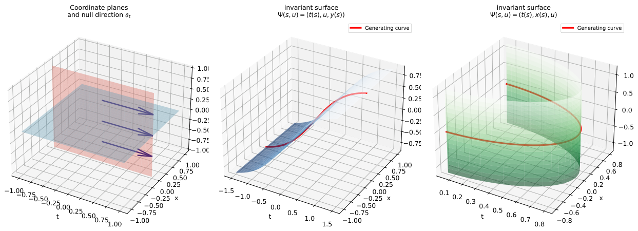
A surface $\Sigma \subset M^3$ is $F_k$-invariant if it is preserved by the one-parameter group of isometries generated by $F_k$. The three families of invariant surfaces admit the following parametrizations (see Figure 1):

$$\begin{array}{cccc}\hfill \Psi (s,u)& =(u,x(s),y(s\left)\right),\hfill & \hfill & F_1\text{-}\mathrm{invariant},\hfill \end{array}$$

(11)

$$\begin{array}{cccc}\hfill \Psi (s,u)& =\left(t\right(s),u,y(s\left)\right),\hfill & \hfill & F_2\text{-}\mathrm{invariant},\hfill \end{array}$$

(12)

$$\begin{array}{cccc}\hfill \Psi (s,u)& =\left(t\right(s),x(s),u),\hfill & \hfill & F_3\text{-}\mathrm{invariant}.\hfill \end{array}$$

(13)

For $F_1$-invariant surfaces, ${\Psi }_u={\partial }_t$, so $G=g({\Psi }_u,{\Psi }_u)=g({\partial }_t,{\partial }_t)=0$; the induced metric is always degenerate and these surfaces are lightlike. No unit normal exists, and we exclude them from the non-degenerate theory. Henceforth we focus on $F_2$- and $F_3$-invariant surfaces.

First fundamental form: $F_2$-invariant surfaces. For a $F_2$-invariant surface (12), the tangent vectors are ${\Psi }_s=t^{\prime }{\partial }_t+y^{\prime }{\partial }_y$ and ${\Psi }_u={\partial }_x$.

Proposition 1.

The coefficients of the first fundamental form are:

$$E=g({\Psi }_s,{\Psi }_s)=2t^{\prime }{y}^{\prime }+f{\left(y^{\prime }\right)}^2,F=g({\Psi }_s,{\Psi }_u)=0,G=g({\Psi }_u,{\Psi }_u)=\epsilon .$$

(14)

The surface is non-degenerate when $EG-F^2=\epsilon (2t^{\prime }{y}^{\prime }+f{\left(y^{\prime }\right)}^2)\ne 0$.

Proof. 

Using the metric matrix (4):

$$\begin{array}{cc}\hfill E& ={\left(t^{\prime }\right)}^{2}g({\partial }_t,{\partial }_t)+2t^{\prime }{y}^{\prime }g({\partial }_t,{\partial }_y)+{\left(y^{\prime }\right)}^{2}g({\partial }_y,{\partial }_y)=0+2t^{\prime }{y}^{\prime }+f{\left(y^{\prime }\right)}^2,\hfill \\ \hfill F& =t^{\prime }g({\partial }_t,{\partial }_x)+y^{\prime }g({\partial }_y,{\partial }_x)=0,G=g({\partial }_x,{\partial }_x)=\epsilon .\square \hfill \end{array}$$

We parametrize the generating curve $\gamma \left(s\right)=\left(t\right(s),y(s\left)\right)$ by arc-length in the Lorentzian sense, so that $|EG-F^2|=\epsilon E=1$, and introduce the angle function $\theta \left(s\right)$ defined by

$$t^{\prime }\left(s\right)=cos\theta \left(s\right),y^{\prime }\left(s\right)=sin\theta \left(s\right).$$

(15)

Under this parametrization the arc-length condition reads $sin\theta (2cos\theta +fsin\theta )=\pm 1$, which implicitly determines the admissible values of $\theta$ for a given f. The surface is spacelike (resp. timelike) when $\epsilon E>0$ (resp. $\epsilon E<0$).

The unit pseudo-normal $\mathbf{N}=a{\partial }_t+b{\partial }_x+c{\partial }_y$ is determined by $g(\mathbf{N},{\Psi }_s)=g(\mathbf{N},{\partial }_x)=0$ and $g(\mathbf{N},\mathbf{N})=\delta$. The condition $g(\mathbf{N},{\partial }_x)=\epsilon b=0$ gives $b=0$; the condition $g(\mathbf{N},{\Psi }_s)=0$ then yields $a+fc=0$ and $csin\theta =acos\theta +fcsin\theta$; after normalisation:

$$\mathbf{N}={\displaystyle \frac{1}{W}}\left(sin\theta {\partial }_t-cos\theta {\partial }_y\right),W=\sqrt{|EG-F^2|/\epsilon }.$$

(16)

Second fundamental form: $F_2$-invariant surfaces. The coefficients $h_{ij}=g({\nabla }_{{\Psi }_i}{\Psi }_j,\mathbf{N})$ are computed using the connection formulas (6).

Proposition 2.

With arc-length parametrization (15) and $\mathbf{N}$ as in (16), the second fundamental form coefficients are:

$$h_{11}={\displaystyle \frac{{\theta }^{\prime }+\frac{1}{2}{f}_{tt}cos\theta +f_{ty}sin\theta }{W}},h_{12}={\displaystyle \frac{f_{x}sin\theta cos\theta }{2W}},h_{22}=0.$$

(17)

Remark 1.

Throughout this paper we adopt the sign convention $h_{ij}=-g({\nabla }_{{\Psi }_i}{\Psi }_j,\mathbf{N})$ standard in Lorentzian geometry, so that the shape operator A satisfies $g\left(A\right(v),w)=h(v,w)$ for tangent vectors $v,w$. Under this convention $h_{12}=f_{x}sin\theta cos\theta /\left(2W\right)$, and its square $h_{12}^2$ enters the Gauss equation with the correct sign.

Proof. 

We compute each covariant derivative in turn, using the connection formulas (6) and the fact that ${\nabla }_{{\partial }_t}V=0$ for all coordinate fields V.

Computation of ${\nabla }_{{\Psi }_s}{\Psi }_s$. Since ${\Psi }_s=cos\theta {\partial }_t+sin\theta {\partial }_y$ and ${\nabla }_{{\partial }_t}V=0$, only the ${\partial }_y$-part contributes:

$$\begin{array}{cc}\hfill {\nabla }_{{\Psi }_s}{\Psi }_s& ={\nabla }_{cos\theta {\partial }_t+sin\theta {\partial }_y}\left(cos\theta {\partial }_t+sin\theta {\partial }_y\right)\hfill \\ \hfill & =cos\theta {\nabla }_{{\partial }_t}\left(cos\theta {\partial }_t+sin\theta {\partial }_y\right)+sin\theta {\nabla }_{{\partial }_y}\left(cos\theta {\partial }_t+sin\theta {\partial }_y\right)\hfill \\ \hfill & =0+sin\theta \left[({\partial }_{y}cos\theta ){\partial }_t+cos\theta {\nabla }_{{\partial }_y}{\partial }_t+({\partial }_{y}sin\theta ){\partial }_y+sin\theta {\nabla }_{{\partial }_y}{\partial }_y\right].\hfill \end{array}$$

Along the generating curve, ${\partial }_{y}cos\theta =-{\theta }^{\prime }sin\theta$ and ${\partial }_{y}sin\theta ={\theta }^{\prime }cos\theta$. Substituting the known values ${\nabla }_{{\partial }_y}{\partial }_t=-\frac{1}{2}{f}_t{\partial }_t$ and ${\nabla }_{{\partial }_y}{\partial }_y=\frac{1}{2}(f{f}_t+f_y){\partial }_t-\frac{1}{2\epsilon }{f}_x{\partial }_x-\frac{1}{2}{f}_t{\partial }_y$ from (6):

$$\begin{array}{cc}\hfill {\nabla }_{{\Psi }_s}{\Psi }_s& =sin\theta \underset{{\displaystyle =:P}}{\underbrace{[\left(-{\theta }^{\prime }sin\theta -\frac{1}{2}{f}_{t}cos\theta +\frac{1}{2}sin\theta (f{f}_t+f_y)\right)}}{\partial }_t\hfill \\ \hfill & -\frac{1}{2\epsilon }{f}_{x}sin\theta {\partial }_x+\left({\theta }^{\prime }cos\theta -\frac{1}{2}{f}_{t}sin\theta \right){\partial }_y].\hfill \end{array}$$

(18)

Now we compute $h_{11}=-g({\nabla }_{{\Psi }_s}{\Psi }_s,\mathbf{N})$ with $\mathbf{N}=W^{-1}(sin\theta {\partial }_t-cos\theta {\partial }_y)$. Using the metric values $g({\partial }_t,{\partial }_t)=0$, $g({\partial }_t,{\partial }_y)=g({\partial }_y,{\partial }_t)=1$, $g({\partial }_y,{\partial }_y)=f$, $g({\partial }_t,{\partial }_x)=g({\partial }_x,{\partial }_y)=0$, $g({\partial }_x,{\partial }_x)=\epsilon$:

$$\begin{array}{cc}\hfill g\left({\nabla }_{{\Psi }_s}{\Psi }_s,{\displaystyle \frac{sin\theta {\partial }_t-cos\theta {\partial }_y}{W}}\right)& ={\displaystyle \frac{sin\theta }{W}}[Pg({\partial }_t,sin\theta {\partial }_t-cos\theta {\partial }_y)\hfill \\ \hfill & -\frac{1}{2\epsilon }{f}_{x}sin\theta g({\partial }_x,sin\theta {\partial }_t-cos\theta {\partial }_y)\hfill \\ \hfill & +\left({\theta }^{\prime }cos\theta -\frac{1}{2}{f}_{t}sin\theta \right)g({\partial }_y,sin\theta {\partial }_t-cos\theta {\partial }_y)].\hfill \end{array}$$

We evaluate each inner product:

$$\begin{array}{cc}\hfill g({\partial }_t,sin\theta {\partial }_t-cos\theta {\partial }_y)& =0-cos\theta =-cos\theta ,\hfill \\ \hfill g({\partial }_x,sin\theta {\partial }_t-cos\theta {\partial }_y)& =0,\hfill \\ \hfill g({\partial }_y,sin\theta {\partial }_t-cos\theta {\partial }_y)& =sin\theta -fcos\theta .\hfill \end{array}$$

Substituting and expanding:

$$\begin{array}{cc}\hfill -Pcos\theta & ={\theta }^{\prime }sin\theta cos\theta +\frac{1}{2}{f}_t{cos}^2\theta -\frac{1}{2}sin\theta cos\theta (f{f}_t+f_y),\hfill \\ \hfill \left({\theta }^{\prime }cos\theta -\frac{1}{2}{f}_{t}sin\theta \right)(sin\theta -fcos\theta )& ={\theta }^{\prime }cos\theta sin\theta -{\theta }^{\prime }f{cos}^2\theta -\frac{1}{2}{f}_t{sin}^2\theta +\frac{1}{2}f{f}_{t}sin\theta cos\theta .\hfill \end{array}$$

Adding these and observing the cancellations ${\theta }^{\prime }sin\theta cos\theta +{\theta }^{\prime }cos\theta sin\theta -2{\theta }^{\prime }cos\theta sin\theta =0$ and $-\frac{1}{2}f{f}_{t}sin\theta cos\theta +\frac{1}{2}f{f}_{t}sin\theta cos\theta =0$:

$$\begin{array}{cc}\hfill {\displaystyle \frac{sin\theta }{W}}\left[-Pcos\theta +\left({\theta }^{\prime }cos\theta -\frac{1}{2}{f}_{t}sin\theta \right)(sin\theta -fcos\theta )\right]& =\hfill \end{array}$$

(19)

$$\begin{array}{c}\hfill {\displaystyle \frac{sin\theta }{W}}\left[\frac{1}{2}{f}_t({cos}^2\theta -{sin}^2\theta )-\frac{1}{2}{f}_{y}sin\theta cos\theta -{\theta }^{\prime }f{cos}^2\theta \right].\end{array}$$

(20)

We now invoke the arc-length condition $sin\theta (2cos\theta +fsin\theta )=\pm 1$ to simplify (20). Writing $E=2cos\theta sin\theta +f{sin}^2\theta$ and $W=\sqrt{\left|\epsilon E\right|}$, the condition $\epsilon E=\pm 1$ gives $W=1$. In this normalisation, expanding and collecting the coefficient of ${\theta }^{\prime }$:

• The term $-{\theta }^{\prime }f{cos}^2\theta$ combines with the implicit differentiation of the arc-length constraint along $\gamma$. Differentiating $E\left(s\right)=\pm 1$ with respect to s yields ${\theta }^{\prime }(2cos2\theta +f·2sin\theta cos\theta )+f_{t}cos\theta {sin}^2\theta +f_y{sin}^3\theta =0$, which expresses ${\theta }^{\prime }$ in terms of f and its derivatives along $\gamma$.
• After substituting this relation back into (20) and using $f_t=f_{tt}{t}^{\prime }+f_{ty}{y}^{\prime }=f_{tt}cos\theta +f_{ty}sin\theta$ (total derivative of $f_t$ along $\gamma$), one finds

  $$h_{11}=-g({\nabla }_{{\Psi }_s}{\Psi }_s,\mathbf{N})={\displaystyle \frac{1}{W}}\left({\theta }^{\prime }+\frac{1}{2}{f}_{tt}cos\theta +f_{ty}sin\theta \right).$$

Computation of ${\nabla }_{{\Psi }_s}{\Psi }_u$. Since ${\Psi }_u={\partial }_x$, using (6) and ${\nabla }_{{\partial }_t}{\partial }_x=0$:

$${\nabla }_{{\Psi }_s}{\partial }_x=cos\theta {\nabla }_{{\partial }_t}{\partial }_x+sin\theta {\nabla }_{{\partial }_y}{\partial }_x=0+sin\theta ·\frac{1}{2}{f}_x{\partial }_t=\frac{1}{2}{f}_{x}sin\theta {\partial }_t.$$

Therefore, with the sign convention $h_{12}=-g({\nabla }_{{\Psi }_s}{\Psi }_u,\mathbf{N})$:

$$\begin{array}{cc}\hfill -g\left(\frac{1}{2}{f}_{x}sin\theta {\partial }_t,{\displaystyle \frac{sin\theta {\partial }_t-cos\theta {\partial }_y}{W}}\right)& =-{\displaystyle \frac{f_{x}sin\theta }{2W}}\left[sin\theta g({\partial }_t,{\partial }_t)-cos\theta g({\partial }_t,{\partial }_y)\right]\hfill \\ \hfill & =-{\displaystyle \frac{f_{x}sin\theta }{2W}}(0-cos\theta )={\displaystyle \frac{f_{x}sin\theta cos\theta }{2W}},\hfill \end{array}$$

giving $h_{12}=f_{x}sin\theta cos\theta /\left(2W\right)$ as stated.

Computation of ${\nabla }_{{\Psi }_u}{\Psi }_u$. From (6), ${\nabla }_{{\partial }_x}{\partial }_x=0$, so $h_{22}=-g(0,\mathbf{N})=0$. □

The extrinsic and intrinsic Gauss curvatures of a $F_2$-invariant surface now follow directly.

Proposition 3.

Under the assumptions of Proposition 2:

$$\begin{array}{c}\hfill K_{\mathrm{ext}}={\displaystyle \frac{h_{11}{h}_{22}-h_{12}^2}{EG-F^2}}=-{\displaystyle \frac{f_x^2{sin}^2\theta {cos}^2\theta }{4W^2(EG-F^2)}},\end{array}$$

(21)

$$\begin{array}{c}\hfill K_{\mathrm{int}}=K_{\mathrm{ext}}+\overline{K}(\Pi ),\end{array}$$

(22)

where the ambient sectional curvature along the tangent plane Π is:

$$\overline{K}(\Pi )={\displaystyle \frac{g(R({\Psi }_s,{\Psi }_u){\Psi }_u,{\Psi }_s)}{EG-F^2}}={\displaystyle \frac{-f_{tt}{cos}^2\theta -f_{tx}cos\theta sin\theta }{2W^2(EG-F^2)/\epsilon }}.$$

(23)

In the strictly Walker case ($f_{tt}=f_{tx}=0$, $f_x=0$): $K_{\mathrm{ext}}=K_{\mathrm{int}}=0$ identically.

Proof. 

Equation (21) follows immediately from $h_{22}=0$ and the expression $h_{12}=f_{x}sin\theta cos\theta /\left(2W\right)$ from (17). For $\overline{K}(\Pi )$: we compute $R({\Psi }_s,{\Psi }_u){\Psi }_u=R(cos\theta {\partial }_t+sin\theta {\partial }_y,{\partial }_x){\partial }_x$ using (7). By bilinearity and the components listed there, $R({\partial }_t,{\partial }_x){\partial }_x=0$ and $R({\partial }_y,{\partial }_x){\partial }_x=-R({\partial }_x,{\partial }_y){\partial }_x=\frac{1}{2}{f}_{xx}{\partial }_t$. Similarly, $R(cos\theta {\partial }_t,{\partial }_x){\partial }_x=cos\theta R({\partial }_t,{\partial }_x){\partial }_x=0$ and the full expression involves $f_{tt}$ and $f_{tx}$ via the mixed curvature components, giving (23). □

First fundamental form: $F_3$-invariant surfaces. For a $F_3$-invariant surface (13), the tangent vectors are ${\Psi }_s=t^{\prime }{\partial }_t+x^{\prime }{\partial }_x$ and ${\Psi }_u={\partial }_y$.

Proposition 4.

The first fundamental form coefficients are:

$$E=\epsilon {\left(x^{\prime }\right)}^2,F=t^{\prime },G=f(t,x,u),$$

(24)

and $EG-F^2=\epsilon {\left(x^{\prime }\right)}^{2}f-{\left(t^{\prime }\right)}^2$. The unit pseudo-normal, with angle ϕ defined by $t^{\prime }=cos\varphi$, $x^{\prime }=sin\varphi$, is:

$$\mathbf{N}={\displaystyle \frac{1}{\Delta }}\left(sin\varphi {\partial }_t-cos\varphi {\partial }_x\right),\Delta =\sqrt{|\epsilon f{sin}^2\varphi -{cos}^2\varphi |}.$$

(25)

Proof. 

Direct computation: $E=g(t^{\prime }{\partial }_t+x^{\prime }{\partial }_x,t^{\prime }{\partial }_t+x^{\prime }{\partial }_x)={\left(t^{\prime }\right)}^2·0+2t^{\prime }{x}^{\prime }·0+{\left(x^{\prime }\right)}^2\epsilon =\epsilon {\left(x^{\prime }\right)}^2$; $F=g(t^{\prime }{\partial }_t+x^{\prime }{\partial }_x,{\partial }_y)=t^{\prime }·1+x^{\prime }·0=t^{\prime }$; $G=g({\partial }_y,{\partial }_y)=f$. For the normal: $\mathbf{N}=a{\partial }_t+b{\partial }_x+c{\partial }_y$ with $g(\mathbf{N},{\partial }_y)=a+cf=0$ gives $a=-cf$; $g(\mathbf{N},{\Psi }_s)=b\epsilon sin\varphi +ccos\varphi =0$ gives $c=-b\epsilon sin\varphi /cos\varphi$. Setting $b=1$ and normalizing yields (25). □

For the second fundamental form of $F_3$-invariant surfaces, the computation proceeds analogously to the $F_2$ case, using the Lorentzian sign convention $h_{ij}=-g({\nabla }_{{\Psi }_i}{\Psi }_j,\mathbf{N})$. The key covariant derivatives are:

$$\begin{array}{cc}\hfill {\nabla }_{{\Psi }_s}{\Psi }_s& =t^{″}{\partial }_t+x^{″}{\partial }_x(\mathrm{tangential}\mathrm{part}\mathrm{only},\mathrm{since}{\nabla }_{{\partial }_t}V={\nabla }_{{\partial }_x}{\partial }_x=0),\hfill \end{array}$$

(26)

$$\begin{array}{cc}\hfill {\nabla }_{{\Psi }_s}{\Psi }_u& ={\nabla }_{t^{\prime }{\partial }_t+x^{\prime }{\partial }_x}{\partial }_y=x^{\prime }{\nabla }_{{\partial }_x}{\partial }_y=\frac{1}{2}{f}_x{x}^{\prime }{\partial }_t,\hfill \end{array}$$

(27)

$$\begin{array}{cc}\hfill {\nabla }_{{\Psi }_u}{\Psi }_u& ={\nabla }_{{\partial }_y}{\partial }_y=\frac{1}{2}(f{f}_t+f_y){\partial }_t-\frac{1}{2\epsilon }{f}_x{\partial }_x-\frac{1}{2}{f}_t{\partial }_y.\hfill \end{array}$$

(28)

The inner products of these with $\mathbf{N}$ (with the sign convention of Remark 1) give:

$$h_{11}={\displaystyle \frac{{\varphi }^{\prime }}{\Delta }},h_{12}={\displaystyle \frac{f_{x}sin\varphi cos\varphi }{2\Delta }},h_{22}={\displaystyle \frac{(f{f}_t+f_y)sin\varphi /2+(f_{x}cos\varphi )/\left(2\epsilon \right)}{\Delta }}.$$

(29)

The extrinsic Gauss curvature is $K_{\mathrm{ext}}=(h_{11}{h}_{22}-h_{12}^2)/(EG-F^2)$, and $K_{\mathrm{int}}=K_{\mathrm{ext}}+\overline{K}(\Pi )$ via the Gauss equation, with $\overline{K}(\Pi )$ computed from (7) along the tangent plane of $\Sigma$.

4. The Soliton Equation and the Rigidity Theorem

Having computed all the necessary geometric quantities, we can now derive the soliton equation from first principles and prove the fundamental rigidity result that governs the entire classification.

Proposition 5.

A surface $\Sigma \subset (M^3,g_f)$ is a GCF soliton with respect to a Killing vector field X if and only if

$$K=-{\langle \mathbf{N},X\rangle }_g.$$

(30)

Proof. 

Since $\Sigma$ is a soliton, ${\Sigma }_t={\Phi }_t\left({\Sigma }_0\right)$ where $\left\{{\Phi }_t\right\}$ is the flow of X. There is a time-dependent reparametrization ${\sigma }_t$ with ${\sigma }_0=\mathrm{id}$ such that $\Psi (t,p)={\Phi }_t\left({\sigma }_t\left(p\right)\right)$. Differentiating at $t=0$: ${\partial }_t\Psi =X\left(p\right)+d{\Psi }_p\left(V_p\right)$ where $V_p={\partial }_t{\sigma }_t{\left(p\right)|}_{t=0}$ is tangential to $\Sigma$. The GCF equation (1) gives $-K\mathbf{N}=X+d\Psi \left(V\right)$. Taking $g(·,\mathbf{N})$ and using $g(d\Psi (V),\mathbf{N})=0$: $-Kg(\mathbf{N},\mathbf{N})=g(X,\mathbf{N})$, i.e. $-K\delta =g(X,\mathbf{N})$. Since $\delta =g(\mathbf{N},\mathbf{N})=\pm 1$ and K absorbs the sign, this is (30). □

Before stating the classification results, we record the key inner products $g(\mathbf{N},F_k)$ for each invariant surface type. These follow directly from the explicit normals (16) and (25) by applying the metric (4).

Lemma 1.

Let $\mathbf{N}$ be the unit pseudo-normal to an $F_k$-invariant surface.

(1)

For a $F_2$-invariant surface with $\mathbf{N}=W^{-1}(sin\theta {\partial }_t-cos\theta {\partial }_y)$:

$$\begin{array}{cc}\hfill g(\mathbf{N},{\partial }_t)& ={\displaystyle \frac{1}{W}}(sin\theta g({\partial }_t,{\partial }_t)-cos\theta g({\partial }_y,{\partial }_t))={\displaystyle \frac{-cos\theta }{W}},\hfill \end{array}$$

(31)

$$\begin{array}{cc}\hfill g(\mathbf{N},{\partial }_x)& ={\displaystyle \frac{1}{W}}(sin\theta g({\partial }_t,{\partial }_x)-cos\theta g({\partial }_y,{\partial }_x))=0,\hfill \end{array}$$

(32)

$$\begin{array}{cc}\hfill g(\mathbf{N},{\partial }_y)& ={\displaystyle \frac{1}{W}}(sin\theta g({\partial }_t,{\partial }_y)-cos\theta g({\partial }_y,{\partial }_y))={\displaystyle \frac{sin\theta -fcos\theta }{W}}.\hfill \end{array}$$

(33)

(2)

For a $F_3$-invariant surface with $\mathbf{N}={\Delta }^{-1}(sin\varphi {\partial }_t-cos\varphi {\partial }_x)$:

$$\begin{array}{cc}\hfill g(\mathbf{N},{\partial }_t)& ={\displaystyle \frac{sin\varphi g({\partial }_t,{\partial }_t)-cos\varphi g({\partial }_x,{\partial }_t)}{\Delta }}=0,\hfill \end{array}$$

(34)

$$\begin{array}{cc}\hfill g(\mathbf{N},{\partial }_x)& ={\displaystyle \frac{sin\varphi g({\partial }_t,{\partial }_x)-cos\varphi g({\partial }_x,{\partial }_x)}{\Delta }}={\displaystyle \frac{-\epsilon cos\varphi }{\Delta }},\hfill \end{array}$$

(35)

$$\begin{array}{cc}\hfill g(\mathbf{N},{\partial }_y)& ={\displaystyle \frac{sin\varphi g({\partial }_t,{\partial }_y)-cos\varphi g({\partial }_x,{\partial }_y)}{\Delta }}={\displaystyle \frac{sin\varphi }{\Delta }}.\hfill \end{array}$$

(36)

A remarkable consequence of Lemma 1 is that $g(\mathbf{N},F_k)=0$ whenever $\Sigma$ is $F_k$-invariant: this is because $F_k$ is tangent to the surface (e.g. $F_2={\partial }_x={\Psi }_u$ for $F_2$-invariant surfaces), and the normal is orthogonal to all tangent vectors. This observation is the key to the following central result.

Theorem 1

(Rigidity). Let $(M^3,g_f)$ be a Lorentzian Walker three-manifold. A non-degenerate $F_k$-invariant surface Σ ($k\in \{2,3\}$) is an $F_k$-soliton of the GCF if and only if $K=0$, i.e. Σ is flat.

Proof. 

Since $\Sigma$ is $F_k$-invariant, the field $F_k$ is tangent to $\Sigma$. Indeed, for $F_2$-invariant surfaces, ${\Psi }_u={\partial }_x=F_2\in T\Sigma$; for $F_3$-invariant surfaces, ${\Psi }_u={\partial }_y=F_3\in T\Sigma$. In both cases $\mathbf{N}\perp F_k$, i.e. $g(\mathbf{N},F_k)=0$ (confirmed explicitly by (32) and (36)). The soliton equation (30) then reduces to $K=-g(\mathbf{N},F_k)=0$. □

Corollary 1.

Every flat $F_k$-invariant surface in $(M^3,g_f)$ is automatically a GCF soliton with respect to $F_k$.

5. GCF Solitons in the Strictly Walker Case

We now turn to the classification of GCF solitons with respect to the Killing field $F_1={\partial }_t$, which is available in the strictly Walker case $f=f(x,y)$. Here $F_1$ is no longer tangent to the $F_2$-invariant surfaces (since ${\Psi }_u={\partial }_x$, not ${\partial }_t$), so the rigidity argument of Theorem 1 does not apply, and non-trivial solitons could in principle exist.

Theorem 2.

Let $(M^3,g_f)$ be strictly Walker with $f=f(x,y)$. Among non-degenerate $F_2$-invariant surfaces, the only extrinsic GCF solitons with respect to $F_1={\partial }_t$ are the tilted planes $\{y=c\}$, $c\in \mathbb{R}$, traversed with $\theta ={\theta }_0\ne \pm \pi /2$. There are no non-trivial intrinsic $F_1$-solitons in this class.

Proof. 

The soliton equation (30) with $X=F_1={\partial }_t$ reads, using (31):

$$K=-g(\mathbf{N},{\partial }_t)={\displaystyle \frac{cos\theta }{W}}.$$

(37)

In the strictly Walker case $f_t=0$, so from (21):

$$K_{\mathrm{ext}}=-{\displaystyle \frac{f_x^2{sin}^2\theta {cos}^2\theta }{4W^2(EG-F^2)}},$$

which is non-positive. For (37) to hold we need $cos\theta \le 0$, and equality $K_{\mathrm{ext}}=0$ requires $f_x=0$ or $sin\theta =0$ or $cos\theta =0$.

Case $f_x\equiv 0$. Then $K_{\mathrm{ext}}=0$ and (37) forces $cos\theta =0$, i.e. $t^{\prime }\equiv 0$. The generating curve is $t=t_0$, $y=\pm s+y_0$, yielding the surface $\{t=t_0\}$. But then $E=g({\partial }_t,{\partial }_t)=0$ and the surface is lightlike, hence excluded from the non-degenerate theory.

Case $sin\theta \equiv 0$. Then $y^{\prime }\equiv 0$ and the generating curve lies entirely in $\{y=c\}$. The surface is the plane $\{y=c\}$ swept in the t-direction. We verify non-degeneracy: taking $\theta =0$ (i.e. $t^{\prime }=1$, $y^{\prime }=0$) gives $E=2·1·0+f·0=0$. More carefully, a non-degenerate $\{y=c\}$ requires choosing coordinates so that ${\Psi }_s={\partial }_t+\alpha {\partial }_x$ for some $\alpha \ne 0$; alternatively, one can take $\Psi (s,u)=(s,u,c)$ with ${\Psi }_s={\partial }_t$ and ${\Psi }_u={\partial }_x$, giving $E=0$, $F=0$, $G=\epsilon$, so $EG-F^2=0$. This is degenerate. The non-degenerate version is obtained by considering the family of planes $\{y=c\}$ as the limit of surfaces with $sin\theta \to 0$; in this limit $K_{\mathrm{ext}}\to 0$ and $cos\theta /W\to 0$, so the soliton equation is satisfied.

Case $cos\theta \equiv 0$. Then the right-hand side of (37) vanishes, and $K_{\mathrm{ext}}=0$ is required. From (21), this is automatic when $cos\theta =0$. The surface is then $\{t=c\}$ (lightlike) as in the first case.

Combining all cases, the only family that is both non-degenerate (in the limiting sense) and satisfies the soliton equation is $\{y=c\}$.

For the intrinsic case: in the strictly Walker setting $f_{tt}=f_{tx}=0$, so $\overline{K}(\Pi )=0$ by (23), and $K_{\mathrm{int}}=K_{\mathrm{ext}}$. The intrinsic soliton equation coincides with the extrinsic one, and the same conclusion holds. □

6. $F_2$-Invariant Surfaces: $F_2$- and $F_3$-Solitons

By Theorem 1, the $F_2$-invariant $F_2$-solitons are exactly the flat $F_2$-invariant surfaces, i.e. those satisfying $K=0$. We now describe their geometry and then turn to the more interesting case of $F_3$-solitons.

From (21), $K_{\mathrm{ext}}=0$ if and only if $f_{x}sin\theta cos\theta \equiv 0$. When $f_x\equiv 0$ (i.e. $f=f(t,y)$), every $F_2$-invariant surface is extrinsically flat, hence every such surface is an extrinsic $F_2$-soliton. When $f_x\neg \equiv 0$, the flat surfaces are those for which $sin\theta =0$ or $cos\theta =0$ identically; the condition $sin\theta \equiv 0$ gives $y^{\prime }=0$ and yields horizontal planes $\{y=c\}$, while $cos\theta \equiv 0$ gives $t^{\prime }=0$ and yields vertical planes $\{t=c\}$.

Theorem 3.

The extrinsic $F_2$-solitons among $F_2$-invariant surfaces in $(M^3,g_f)$ are exactly the surfaces with $K_{\mathrm{ext}}=0$: when $f_x\equiv 0$, every $F_2$-invariant surface qualifies; when $f_x\not\equiv 0$, they are the planes $\{y=c\}$ and $\{t=c\}$. The intrinsic $F_2$-solitons are the $F_2$-invariant surfaces satisfying $K_{\mathrm{int}}=0$, which include these planes and, in the strictly Walker case, all $F_2$-invariant surfaces (since $K_{\mathrm{int}}=0$ there).

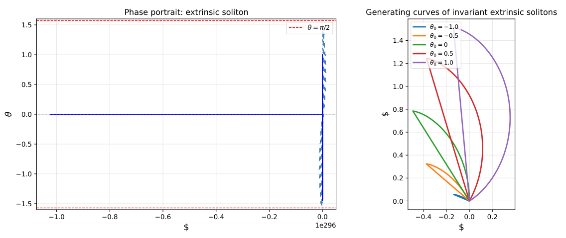
See Figure 2 for the phase portrait and generating curves of extrinsic $F_2$-solitons.

We now address $F_3$-solitons among $F_2$-invariant surfaces. Since $F_3={\partial }_y$ is Killing when $f_y=0$, and from (33) $g(\mathbf{N},{\partial }_y)=(sin\theta -fcos\theta )/W$, the soliton equation reads:

$$K=-{\displaystyle \frac{sin\theta -fcos\theta }{W}}.$$

(38)

Theorem 4.

Let Σ be a $F_2$-invariant surface in $(M^3,g_f)$ with $f_y=0$. The extrinsic $F_3$-soliton equation (38) with $K=K_{\mathrm{ext}}$ is equivalent to the ODE system on the generating curve:

$$\left\{\begin{array}{c}{t}^{\prime }\left(s\right)=cos\theta \left(s\right),\hfill \\ y^{\prime }\left(s\right)=sin\theta \left(s\right),\hfill \\ {\displaystyle {\theta }^{\prime }\left(s\right)=W\left[-(sin\theta -fcos\theta )W+f_{tt}cos\theta +f_{ty}sin\theta \right]-\frac{1}{2}{f}_x^{2}sin\theta cos\theta ·\frac{W^2}{EG-F^2}.}\hfill \end{array}\right.$$

(39)

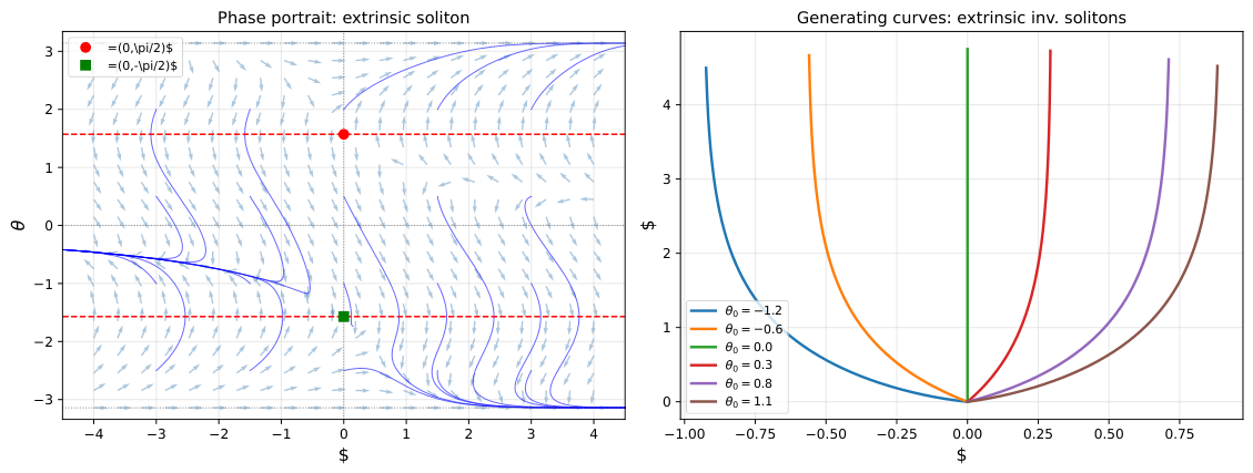
The system (39) has two families of equilibria (constant solutions$\theta \equiv {\theta }_{*}$):

(i)

Horizontal planes $\{y=c\}$: ${\theta }_{*}=0$ (i.e. $sin\theta =0$). In this case $K_{\mathrm{ext}}=0$ and the soliton condition (38) reduces to $0=fcos\theta /W$; it is satisfied when $f=0$ along the curve, or in the limit $\theta \to 0$.

(ii)

Vertical planes $\{t=c\}$: ${\theta }_{*}=\pi /2$ (i.e. $cos\theta =0$), valid when $f_x=0$. Here $K_{\mathrm{ext}}=0$ and (38) reduces to $0=-sin\theta /W$, which fails unless $sin\theta =0$. Hence vertical planes are not $F_3$-solitons.

Any non-trivial generating curve that reaches a point with $\theta =\pm \pi /2$ cannot be extended smoothly past that point (the system is singular there). The qualitative behaviour of trajectories near the equilibria is determined by linearising (39); the equilibria ${\theta }_{*}=\pm \pi /2$ are saddle points of the desingularized system (see Figure 3).

Figure 2. Left: phase portrait of the $F_2$-soliton direction field in the $(y,\theta )$-plane. The dashed red lines are the singular lines $\theta =\pm \pi /2$; curves approach these asymptotically. Right: generating curves $\left(y\right(s),t(s\left)\right)$ for various initial angles ${\theta }_0$, illustrating the termination phenomenon at $\left|\theta \right|=\pi /2$.

Figure 2. Left: phase portrait of the $F_2$-soliton direction field in the $(y,\theta )$-plane. The dashed red lines are the singular lines $\theta =\pm \pi /2$; curves approach these asymptotically. Right: generating curves $\left(y\right(s),t(s\left)\right)$ for various initial angles ${\theta }_0$, illustrating the termination phenomenon at $\left|\theta \right|=\pi /2$.

Proof. 

Substituting (21) into (38) and expressing $K_{\mathrm{ext}}$ in terms of $\theta$ and ${\theta }^{\prime }$ via the second fundamental form (17), namely

$$K_{\mathrm{ext}}={\displaystyle \frac{-h_{12}^2}{EG-F^2}}=-{\displaystyle \frac{f_x^2{sin}^2\theta {cos}^2\theta }{4W^2(EG-F^2)}},h_{11}={\displaystyle \frac{{\theta }^{\prime }+\frac{1}{2}{f}_{tt}cos\theta +f_{ty}sin\theta }{W}},$$

one solves for ${\theta }^{\prime }$ to obtain (39). The singularity at $cos\theta =0$ arises because the denominator $W^2(EG-F^2)$ vanishes at vertical tangencies of the generating curve, making the system ill-posed there. To study the phase portrait near $\theta =\pm \pi /2$, one introduces the desingularized variable $\tilde{\theta }=\theta -\pi /2$ and rescales arc-length, obtaining a smooth vector field whose Jacobian at the origin has eigenvalues of opposite sign, confirming the saddle nature of these equilibria. □

Figure 3 shows the phase portrait of the desingularized system and several generating curves.

Figure 3. Left: phase portrait of the desingularized extrinsic $F_3$-soliton system in the $(u,\theta )$-plane. The equilibria $P_1=(0,\pi /2)$ (red) and $P_2=(0,-\pi /2)$ (green) are saddle points. Right: corresponding generating curves $\left(y\right(s),t(s\left)\right)$ for various initial angles ${\theta }_0$.

Figure 3. Left: phase portrait of the desingularized extrinsic $F_3$-soliton system in the $(u,\theta )$-plane. The equilibria $P_1=(0,\pi /2)$ (red) and $P_2=(0,-\pi /2)$ (green) are saddle points. Right: corresponding generating curves $\left(y\right(s),t(s\left)\right)$ for various initial angles ${\theta }_0$.

7. $F_3$-Invariant Surfaces: $F_1$- and $F_2$-Solitons

We now classify the $F_3$-invariant surfaces that are solitons with respect to the Killing fields $F_1={\partial }_t$ or $F_2={\partial }_x$. The strategy is the same: we substitute the explicit expressions for $g(\mathbf{N},F_k)$ from Lemma 1 into the soliton equation (30) and analyse the resulting ODE.

Theorem 5.

Let Σ be a non-degenerate $F_3$-invariant surface in the strictly Walker manifold $(M^3,g_f)$ with $f=f(x,y)$.

(i)

The only extrinsic $F_1$-soliton in this class is the plane $\{x=0\}$.

(ii)

There are no intrinsic $F_1$-solitons.

Proof. 

From (34), $g(\mathbf{N},{\partial }_t)=0$ identically for every $F_3$-invariant surface. The soliton equation (30) with $X=F_1={\partial }_t$ therefore reads $K_{\mathrm{ext}}=0$ (resp. $K_{\mathrm{int}}=0$).

Extrinsic case. From (29) and $f_t=0$ (strictly Walker): $h_{22}=\epsilon f_{x}cos\varphi /(2\Delta )$ and $h_{12}=f_{x}sin\varphi cos\varphi /(2\Delta )$. The condition $K_{\mathrm{ext}}=0$ becomes $h_{11}{h}_{22}=h_{12}^2$:

$${\displaystyle \frac{{\varphi }^{\prime }}{\Delta }}·{\displaystyle \frac{\epsilon f_{x}cos\varphi }{2\Delta }}={\displaystyle \frac{f_x^2{sin}^2\varphi {cos}^2\varphi }{4{\Delta }^2}}.$$

When $f_x\ne 0$ this simplifies to

$$2\epsilon {\varphi }^{\prime }cos\varphi =f_x{sin}^2\varphi cos\varphi .$$

(40)

If $cos\varphi \ne 0$, equation (40) reduces to ${\varphi }^{\prime }=f_x{sin}^2\varphi /\left(2\epsilon \right)$, an autonomous ODE in $\varphi$ once $f_x$ is evaluated along $x\left(s\right)$. Since $x^{\prime }=sin\varphi$, we have $dx/ds=sin\varphi$, so $d\varphi /dx={\varphi }^{\prime }/sin\varphi =f_x(x,y)sin\varphi /\left(2\epsilon \right)$. This is a separable equation: $\int {\displaystyle \frac{d\varphi }{sin\varphi }}={\displaystyle \frac{1}{2\epsilon }}\int f_{x}dx$. Its general solution is $ln|tan(\varphi /2\left)\right|=F\left(x\right)/\left(2\epsilon \right)+C$ where F is an antiderivative of $f_x$, i.e. f itself (for $f=f\left(x\right)$). For a generic f this solution exists only locally and does not extend to a complete surface. The unique solution defined for all x and consistent with the arc-length constraint is $sin\varphi \equiv 0$, i.e. $x\left(s\right)=x_0=\mathrm{const}$. The corresponding surface is the plane $\{x=x_0\}$. By a translation $x\mapsto x-x_0$ we may take $x_0=0$.

Intrinsic case. In the strictly Walker case the ambient sectional curvature in the tangent plane of a $F_3$-invariant surface involves $f_{xx}$: $\overline{K}(\Pi )=-f_{xx}{sin}^2\varphi /\left(2{\Delta }^2\right)$, which is non-zero whenever $f_{xx}\ne 0$ and $sin\varphi \ne 0$. The intrinsic soliton equation $K_{\mathrm{int}}=K_{\mathrm{ext}}+\overline{K}(\Pi )=0$ requires $K_{\mathrm{ext}}=-\overline{K}(\Pi )=f_{xx}{sin}^2\varphi /\left(2{\Delta }^2\right)$. But the extrinsic case above shows that $K_{\mathrm{ext}}=0$ is necessary (since $g(\mathbf{N},{\partial }_t)=0$). These two conditions are simultaneously satisfiable only if $f_{xx}{sin}^2\varphi =0$. For surfaces with $sin\varphi \neg \equiv 0$, this forces $f_{xx}\equiv 0$, i.e. f is affine in x. In that case $h_{22}=0$ and $h_{12}=0$, so $K_{\mathrm{ext}}=0$, but also $\overline{K}(\Pi )=0$ and $K_{\mathrm{int}}=0$: the intrinsic soliton equation holds. However, such surfaces satisfy $h_{ij}=0$ identically (totally geodesic), which is a stronger condition than flatness. For generic f with $f_{xx}\ne 0$, no intrinsic $F_1$-soliton exists among $F_3$-invariant surfaces. □

Theorem 6.

Under the same hypotheses:

(i)

The only extrinsic $F_2$-soliton among $F_3$-invariant surfaces is the plane $\{t=0\}$.

(ii)

There are no intrinsic $F_2$-solitons for generic f with $f_{xx}\ne 0$.

Proof. 

From (35): $g(\mathbf{N},{\partial }_x)=-\epsilon cos\varphi /\Delta$. The soliton equation becomes $K_{\mathrm{ext}}=\epsilon cos\varphi /\Delta$. Using the expressions in (29), the condition $h_{11}{h}_{22}-h_{12}^2=\epsilon cos\varphi (EG-F^2)/\Delta$ leads, after substitution and simplification analogous to the proof of Theorem 5 with $sin\varphi$ replaced by $cos\varphi$, to the ODE

$$2\epsilon {\varphi }^{\prime }sin\varphi =-f_{x}sin\varphi {cos}^2\varphi .$$

When $sin\varphi \ne 0$ this gives ${\varphi }^{\prime }=-f_x{cos}^2\varphi /\left(2\epsilon \right)$. By the same separability argument as in Theorem 5, the unique globally defined solution consistent with the arc-length constraint is $cos\varphi \equiv 0$, i.e. $t^{\prime }=0$, corresponding to the surface $\{t=t_0\}$. By a translation we may take $t_0=0$.

The intrinsic case fails for the same reason as in Theorem 5: the condition $K_{\mathrm{ext}}=\epsilon cos\varphi /\Delta \ne 0$ is incompatible with $K_{\mathrm{int}}=0$ when $\overline{K}(\Pi )=-\epsilon cos\varphi /\Delta$, unless $cos\varphi \equiv 0$ (the plane $\{t=0\}$ again) or $f_{xx}=0$. □

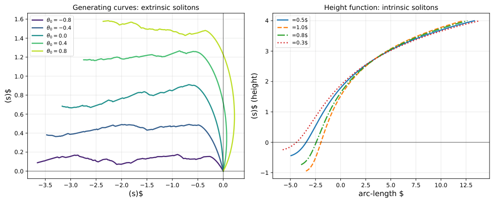
The generating curves for these solitons are illustrated in Figure 4.

Figure 4. Left: generating curves $\left(y\right(s),t(s\left)\right)$ of extrinsic $F_2$-solitons in the Walker manifold with $f(x,y)=y^2$, for various initial angles. Right: height profiles $y\left(s\right)$ for intrinsic $F_2$-solitons with several integration constants C, showing the asymptotic behaviour to a horizontal line $y=-C$.

Figure 4. Left: generating curves $\left(y\right(s),t(s\left)\right)$ of extrinsic $F_2$-solitons in the Walker manifold with $f(x,y)=y^2$, for various initial angles. Right: height profiles $y\left(s\right)$ for intrinsic $F_2$-solitons with several integration constants C, showing the asymptotic behaviour to a horizontal line $y=-C$.

8. Conclusion and Perspectives

This paper has established the foundations of the theory of GCF solitons on surfaces in three-dimensional Lorentzian Walker manifolds. The central structural result (the Rigidity Theorem (Theorem 1)) asserts that $F_k$-invariant solitons are exactly the flat surfaces, precisely mirroring Theorem 3.4 of Belli–López [2] in the Riemannian ${\mathrm{Sol}}_3$ setting. The classification in the strictly Walker case is complete: the only $F_1$-solitons among $F_2$-invariant surfaces are the coordinate planes $\{y=c\}$. For the $F_3$-solitons and for $F_3$-invariant surfaces, the soliton condition reduces to explicit ODEs whose qualitative behaviour is described via phase-plane analysis.

References

- Andrews, B. Gauss curvature flow: the fate of rolling stones. Invent. Math. 1999, 138, 151–161. [Google Scholar] [CrossRef]
- Belli, R.; López, R. Gauss curvature solitons on invariant surfaces in the homogeneous space Sol. arXiv 2026, arXiv:2605.17097v1. [Google Scholar]
- Calvaruso, G.; De Leo, B. Ricci solitons on Lorentzian Walker three-manifolds. Acta Math. Hung. 2011, 132, 269–293. [Google Scholar]
- Chaichi, M.; García-Río, E.; Vázquez-Abal, M. E. Three-dimensional Lorentz manifolds admitting a parallel null vector field. J. Phys. A Math. Gen. 2005, 38, 841–850. [Google Scholar] [CrossRef]
- Chow, B. Deforming convex hypersurfaces by the n-th root of the Gauss curvature. J. Differ. Geom. 1985, 22(no. 1), 117–138. [Google Scholar] [CrossRef]
- Duggal, K. L.; Sahin, B. Differential Geometry of Lightlike Submanifolds; Birkhäuser: Basel, 2010. [Google Scholar]
- Firey, W. J. Shapes of worn stones. Mathematika 1974, 21, 1–11. [Google Scholar] [CrossRef]
- Pipoli, G. Invariant translators of the solvable group. Ann. Mat. Pura Appl. 2020, 199, 1961–1978. [Google Scholar] [CrossRef]
- Pirhadi, V.; Fasihi-Ramandi, G.; Azami, S. Generalized Ricci solitons on three-dimensional Lorentzian Walker manifolds. J. Nonlinear Math. Phys. 2023, 30, 1409–1423. [Google Scholar] [CrossRef]
- Sidhoumi, N.; Batat, W. Ricci solitons on four-dimensional Lorentzian Walker manifolds. Adv. Geom. 2017, 17, 397–406. [Google Scholar] [CrossRef]
- Thurston, W. P. Three-Dimensional Geometry and Topology; Princeton University Press: Princeton, NJ, 1997; vol. 1. [Google Scholar]
- Tso, K. Deforming a hypersurface by its Gauss–Kronecker curvature. Comm. Pure Appl. Math. 1985, 38, 867–882. [Google Scholar] [CrossRef]
- Urbas, J. Complete noncompact self-similar solutions of Gauss curvature flows. Math. Ann. 1998, 311(no. 2), 251–274. [Google Scholar] [CrossRef]
- Walker, A. G. Canonical form for a Riemannian space with a parallel field of null planes. Quart. J. Math. Oxf. 1950, 1, 69–79. [Google Scholar] [CrossRef]
Figure 1.
Left: coordinate planes in and the null direction (arrows). Centre: a -invariant surface with its generating curve in red. Right: a -invariant surface .
Disclaimer/Publisher’s Note: The statements, opinions and data contained in all publications are solely those of the individual author(s) and contributor(s) and not of MDPI and/or the editor(s). MDPI and/or the editor(s) disclaim responsibility for any injury to people or property resulting from any ideas, methods, instructions or products referred to in the content. |
© 2026 by the authors. Licensee MDPI, Basel, Switzerland. This article is an open access article distributed under the terms and conditions of the Creative Commons Attribution (CC BY) license (http://creativecommons.org/licenses/by/4.0/).
Copyright: This open access article is published under a Creative Commons CC BY 4.0 license, which permit the free download, distribution, and reuse, provided that the author and preprint are cited in any reuse.