

Submitted:
27 May 2026
Posted:
28 May 2026
You are already at the latest version
Abstract
Background: Multi-Agent Path Finding (MAPF) has been widely studied in recent years. However, the computational cost of solving MAPF and MAPF for large agents (LA-MAPF) grows exponentially as the number of agents increases. This challenge is particularly severe for LA-MAPF, primarily due to the increased overhead of conflict detection between geometric agents. Objectives: To reduce the computational cost of solving MAPF and LA-MAPF problems, a general method is needed that can accelerate a variety of MAPF algorithms. Methods: We propose a framework that decomposes an LA-MAPFproblem into multiple subproblems, which are solved independently to reduce computational costs. The framework is general and compatible with various MAPF algorithms (e.g., CBS or LaCAM). The decomposition of an LA-MAPF problem is formulated as a combinatorial optimization problem and solved using neighborhood search. To handle unsolvable subproblems generated during decomposition, we introduce a solvability safeguard mechanism that merges subproblems until all are solvable. Results: Our experiments demonstrate the performance of the framework across various mapsasthenumberofagentsincreases, showing substantial acceleration of both MAPF and LA-MAPF methods. Specifically, after applying Break Loops, the average runtime of CBS and LA-CBS is reduced from 49.0 s to 6.8 s and from 54.0 s to 18.65 s, respectively; LaCAM and LA-LaCAM are reduced from 9.5 s to 7.0 s and from 52.9 s to 16.2 s, respectively. The success rate of CBS and LA-CBS increases from 0.27 to 0.98 and from 0.11 to 0.72, respectively; LaCAM and LA-LaCAM increase from 0.85 to 0.97 and from 0.10 to 0.77, respectively. Conclusions: Our results show that incorporating Break Loops into MAPF and LA-MAPF methods significantly reduces computational costs and improves success rates. These f indings demonstrate that solving MAPF problems can be accelerated by decomposing them into subproblems. To facilitate further research, we have made the source code for the framework publicly available at https://github.com/JoeYao-bit/LayeredMAPF/tree/main/algorithm/LA-MAPF.
Keywords:
multi-agent path finding
1. Introduction
In robotics and computer games, multiple agents often need to move simultaneously, and avoiding conflicts between agents has led to the study of Multi-Agent Path Finding (MAPF). MAPF aims to find a path for each agent from its start state to its target state on a given map, ensuring that no agents collide at any time. Numerous MAPF algorithms have been developed in recent years, such as Conflict-Based Search (CBS) [1], Priority-Based Search (PBS) [2], Priority Inheritance with Backtracking (PIBT) [3], and Lazy Constraints Addition for MAPF (LaCAM) [4].
Although previous MAPF algorithms have been applied in some real-world contexts [5,6,7], they are based on a simplifying assumption that limits their applicability. This assumption treats agents as point agents, which occupy exactly one cell at any time, ignoring their actual shape. In reality, agents are geometric with definite shapes (e.g., rectangular or circular), and typically occupy a set of points at any given time. Li et al. [8] refer to such agents as large agents. MAPF algorithms can be applied to large agents by lowering the resolution of the environment’s discretization. However, this approach degrades performance and reduces practical applicability. Therefore, Li et al. [8] formalize and study LA-MAPF, i.e., MAPF for large agents.
Empirical evidence indicates that LA-MAPF is more time-consuming than classic MAPF, as LA-MAPF needs more computational resources to determine whether two agents have conflicts (the definition of conflicts can be found in Section 3). For example, one of the SOTA (state-of-the-art) MAPF methods, LaCAM [4] (one of the fastest MAPF methods), is capable of solving a MAPF problem with 1000 agents in 60 seconds, whereas LA-LaCAM can only solve a LA-MAPF problem with 20 to 30 agents in 60 seconds (on the same map and computation platform). Therefore, reducing the time cost of solving the MAPF problem to enable LA-MAPF to find a solution involving more agents is crucial.
Motivated by the observation that the computational cost of optimally solving MAPF problems grows exponentially with the number of agents [9], we proposed a decomposition approach for MAPF problems [10] in our previous work. This method iteratively bipartitions MAPF problems until no smaller subproblems remain, as illustrated in Figure 1. Subsequently, all subproblems are solved independently and their solutions are merged to obtain a solution to the original problem. The merging is implemented by adding wait actions to ensure that solutions from different subproblems have no conflicts. Experimental results demonstrate that this decomposition significantly reduces the time cost and memory usage required to solve MAPF problems.
However, this approach has several limitations. First, it does not guarantee that every generated subproblem is solvable, which may cause the method to fail even on originally solvable MAPF instances. Second, the bipartition process considers only the agents within the current subproblem rather than all agents globally, leaving room for further decomposition into smaller subproblems.
To address these issues, we propose a novel framework for MAPF problem decomposition that is formulated as a combinatorial optimization problem. It considers all agents during the decomposition process, thereby enabling the generation of smaller subproblems. Inspired by Independence Detection [11], we further introduce a solvability safeguard to ensure that all generated subproblems are eventually solvable. In the worst case, the safeguard merges all subproblems back into the original problem and solves it using the underlying MAPF method.
The main contributions of this article are as follows:
1. We formulate the decomposition of LA-MAPF problems as a combinatorial optimization problem and solve it using a neighborhood search algorithm.
2. We propose a general framework that enables LA-MAPF methods to solve subproblems independently and merge their solutions into a conflict-free solution to the original problem. The framework includes a solvability safeguard mechanism that iteratively merges unsolvable subproblems until all subproblems become solvable.
3. We conduct extensive experiments to evaluate the effectiveness of the proposed decomposition across various maps and increasing numbers of agents. We assess its impact on LA-MAPF and MAPF methods in terms of computational time, success rate, and solution quality (makespan and sum of costs).
It is worth noting that MAPF is a simplified version of LA-MAPF; therefore, our framework can also be applied to standard MAPF problems. By replacing the conflict detection module in our framework with the conflict detection mechanism used in MAPF, the framework can be directly adapted to MAPF settings. However, some MAPF methods (e.g., LaCAM [4]) are already highly efficient and can handle MAPF instances with thousands of agents. As a result, applying our framework to such methods does not lead to significant performance improvements.
Consequently, in this manuscript, we mainly focus on LA-MAPF problems, where conflict detection between large agents is substantially more time-consuming. In this context, our framework can significantly reduce the overall computational cost. More detailed comparisons of our framework and LaCAM on both MAPF and LA-MAPF problems are presented in the Results section.
The remainder of this article is organized as follows. In the Related work section, we review related articles on the decomposition of MAPF problems. In the Preliminaries section, we introduce basic concepts and processes, followed by our method in the Methodology section. This section introduces how we decompose the MAPF problem into subproblems and merge their solutions to obtain a solution to the original problem. Our test results on the performance of the decomposition under various maps and different numbers of agents are presented in the Results section, along with an examination of how decomposition improves LA-MAPF methods. It also compares our new method with our previous method. Finally, the Conclusion section concludes the article.
2. Related Work
2.1. MAPF for Large Agents
Li et al. [8] generalized MAPF to LA-MAPF (MAPF for Large Agents), which considers the shapes of agents. In LA-MAPF, each agent has a fixed geometric shape around a reference point that cannot undergo transformations such as rotations. Therefore, different agents have different traversable subgraphs because of their different shapes. Li et al. [8] adapted CBS (Conflict-Based Search) to LA-CBS (CBS for Large Agents) to find a set of conflict-free paths that move all agents from their start vertices to their goal vertices while minimizing the sum of costs of all paths. To the best of our knowledge, this is the first study to focus on MAPF for agents with different shapes.
To accelerate LA-CBS, Zhang et al. [12] introduce mutex propagation and its concomitant symmetry-breaking to LA-CBS. The algorithm first finds mutexes between MDDs (Multi-Decision Diagrams) of a pair of agents via mutex propagation. Then, it uses these mutexes to identify and automatically resolve cardinal conflicts. The results show that this technique significantly improves the performance of some LA-CBS-based methods in terms of both success rate and runtime. Compared with this technique, our method is not limited to CBS-based methods but can be applied to any classic MAPF methods.
2.2. Related Work to LA-MAPF
Like LA-MAPF, Wen et al. [13] presented a mathematical formalization of the Multi-Agent Path Finding for Car-Like robots (CL-MAPF) problem. This approach considers both the position and orientation of car-like robots. It proposes a novel hierarchical search-based solver called Car-Like Conflict-Based Search to address this problem. It applies a body conflict tree to address conflicts while considering the shapes of the agents. It also introduces a new algorithm called Spatiotemporal Hybrid-State A* as the single-agent planner to generate agent paths satisfying both kinematic and spatiotemporal constraints.
Bai et al. [14] introduced the Heterogeneous Conflict Based Search (HCBS) algorithm as a solution to the Multi-Agent Pathfinding (MAPF) problem in nonholonomic heterogeneous robot scenarios. Leveraging the foundational principles of CBS, HCBS adapts to the diversity of robotic agents by implementing distinct path-planning strategies and incorporating a body conflict detection mechanism for conflict avoidance. Additionally, it introduces two suboptimal derivatives of HCBS—Enhanced HCBS (EHCBS) and Depth-First HCBS (DFHCBS), aimed at improving computational efficiency. While EHCBS tends to be less computationally efficient than HCBS in scenarios with fewer than 20 agents, owing to the overhead of managing additional focal lists, its performance surpasses that of HCBS in more densely populated maps. Conversely, DFHCBS consistently outperforms HCBS in terms of computational speed across all tested scenarios.
2.3. Existing Work on the Decomposition of MAPF Problems
The idea of splitting a MAPF problem into multiple smaller subproblems has been explored by researchers in recent years. Standley et al. [15,16] proposed that if the optimal paths of two agents have no conflicts (in classic MAPF, there are two types of conflicts: vertex conflict (i.e., node conflict), in which two agents visit the same node, and edge conflict, in which two agents visit the same edge in opposite directions; LA-MAPF’s conflict definition can be found in the Preliminaries section), they can be solved independently. Standley [16] introduced the Independence Detection (ID) algorithm to decompose a group of agents into the smallest possible groups. ID first assigns each agent to its own group and finds an initial path for each group independently. It then attempts to find alternative paths to avoid conflicts. If these attempts to find conflict-free paths fail, ID merges the conflicting groups. The process continues until there are no conflicts between agents from different groups.
While ID ensures the solvability of the decomposition, searching the full paths multiple times is very time-consuming. In contrast, our method reduces the time cost of decomposition by using a connectivity graph, which represents connections between regions, instead of cell-by-cell paths. Thus, our method is theoretically more efficient. Additionally, ID does not consider how the order of solving affects whether two agents are independent (e.g., by altering the order of solving, two agents can be solved separately, even if their isolated paths initially have conflicts).
Sharon et al. [17] proposed a continuum between CBS (Conflict-Based Search) and ID called Meta-Agent CBS (MA-CBS). MA-CBS introduces a predefined parameter B, where conflicting agents are merged into a meta-agent and treated as a joint composite agent if the number of conflicts exceeds B. The original CBS algorithm corresponds to the extreme case where B = ∞ (never merges agents), whereas the Independence Detection (ID) framework [15,16] represents the other extreme, where B = 0 (always merges agents when conflicts occur).
Prioritized Planning (PP) [18] decomposes a MAPF problem into multiple subproblems, each associated with a unique priority and containing a single agent. Paths are planned sequentially from the highest-priority agent to the lowest. For each agent, a path is computed that avoids static obstacles as well as the trajectories of higher-priority agents planned in earlier iterations. PP terminates with either success or failure within at most n iterations.
However, PP does not guarantee the existence of solutions that avoid both the start states of lower-priority agents and the regions occupied by higher-priority agents, rendering it incomplete.
To address this issue, Michal et al. [19] suggested well-formed infrastructures (i.e., limitations on the distribution of obstacles, start states, and target states) to ensure that the problem can be solved by priority-based search in all cases. A well-formed infrastructure is defined as one in which the endpoints (the start and target states of each agent) are distributed such that no agent standing on an endpoint can completely prevent other agents from moving between any two other endpoints.
Priority-Based Search (PBS) [2] is an incomplete, suboptimal algorithm designed for prioritized planning. At the high level, PBS employs a depth-first search to dynamically construct a priority ordering, forming a priority tree (PT). When a conflict occurs, PBS greedily assigns a higher priority to one of the agents involved. It efficiently backtracks and explores alternative branches only when no solution is found in the current branch. In this way, PBS incrementally builds a single partial priority ordering until all conflicts are resolved.
Once each agent is assigned a unique priority, PBS computes a minimum-cost path (in priority order) from the agent’s starting state to its target state, ensuring that it does not collide with the paths of higher-priority agents that have already been planned.
PBS ranks among the most efficient methods for solving MAPF. However, prioritized planning with an arbitrary priority ordering does not guarantee completeness or optimality in general [2]. In contrast, while our method cannot always solve each agent separately, it introduces a solvability safeguard to ensure that there is no unsolvable subproblem.
3. Preliminaries
In this section, we introduce the basic concepts of our framework.
3.1. Workspace
Definition 1.
Workspace: An -dimensional Euclidean space (typically, or 3). Each cell (or element) in can be in one of two states: passable or unpassable. The set of all passable cells is denoted by , and the set of all unpassable cells is denoted by .
3.2. Agent State
We define the agent state as a tuple of location and orientation.
Definition 2.
Location: The location is a point in the Euclidean space and is specified by its coordinates , where for .
In an -dimensional Euclidean space, we define possible orientations. Each orientation is a unit vector along one of the coordinate axes.
For example:
- In a 2D space, the four possible orientations are , , , and (i.e., east, west, north, south).
- In a 3D space, the six possible orientations are , , , , , and (i.e., east, west, north, south, up, down).
Definition 3.
Agent Orientation: The orientation of an agent is defined as an integer r, where . Each value of r corresponds to one of the possible orientations in an -dimensional space. Orientation is important with respect to shaped agents as changing orientation changes occupied grids.
For example:
- In a 2D space, corresponds to the orientation , corresponds to , corresponds to , and corresponds to .
- In a 3D space, corresponds to the orientation , corresponds to , corresponds to , and so on up to , which corresponds to .
By considering orientation changes during planning, we can account for conflicts arising from these changes, making our solutions more realistic than those of approaches that consider only locations. Our approach thus makes solutions more transferable to real-world scenarios and makes them more convenient for execution.
Definition 4.
Robot’s State
is defined as . For convenience, we denote the start state of agent as and the target state as .
As mentioned by Li et al. [8], each agent has a fixed geometric shape centered around a reference point, which does not change position during rotations. We say that an agent is in state s when its reference point is located at the position specified by s, and its orientation matches the orientation defined in s.
3.3. Conflict Detection
Considering that different agents have different shapes, we define the process for checking whether agents collide with obstacles or with other agents. To facilitate conflict checks for arbitrary shapes, we discretize these shapes into cells. Next, we check whether the cells of the shapes overlap with the cells of the obstacles or the cells occupied by other agents’ shapes. Examples of this process are shown in Figure 2.
Considering that most agents are located far from other agents and obstacles during path planning, we introduce optimizations to avoid unnecessary conflict checks. We perform conflict detection between an agent and the map only if the agent’s distance to the nearest obstacle is between its circumcircle radius and its inscribed circle radius. Additionally, we perform conflict detection between agents only if the distance between their centers is between the sum of their circumcircle radii and the sum of their inscribed circle radii. If the distance is larger than the circumcircle radius, the configuration is guaranteed to be conflict-free; if the distance is smaller than the inscribed circle radius, a conflict is inevitable, and no further precise conflict detection is required.
Definition 5.
We denote the cells occupied by agent at the robot state s as and the cell occupied by when it transitions from to as . If , then agent at state s collides with obstacles. If , then agent collides with obstacles when it transitions from to .
In the implementation, we do not explicitly compute during conflict detection. Instead, we precompute the cells occupied by each action (e.g., for a 2D MAPF problem, there are three actions: move forward, turn left, and turn right) of every agent during the initialization stage. Then, when conflict detection is required, we look up this table and apply a coordinate transformation to obtain .
This conflict detection strategy may lose some details of the agents’ shapes; however, we adopt this approach to reduce the time cost of conflict detection, as conflict detection accounts for a major portion of the overall time cost of LA-MAPF.
3.4. Actions
To adapt to mobile platforms as much as possible, we only allow three types of actions: waiting at the current state, moving forward, or rotating by 90 degrees to an orthogonal direction. All actions have unit cost.
3.5. Subgraph of an Agent
As mentioned by Li et al. [8], different agents have different traversable subgraphs due to their varying shapes.
Definition 6.
Subgraph : A directed graph that represents all feasible states and valid transitions for agent . The vertex set includes all collision-free agent states, and the edge set contains all collision-free transitions between states. Specifically, for every , the condition must hold, meaning the agent does not collide with obstacles at state v. Similarly, for every directed edge , the transition satisfies , indicating no collision with obstacles during movement. Here, denotes a vertex (state), and denotes a valid transition from state v to .
To ensure that a LA-MAPF problem is solvable, the start state and target state of each agent must be connected by at least one valid path within its subgraph. When constructing the subgraph, only the agent’s own geometric shape and the static map (i.e., the workspace) are considered—other agents are ignored during this phase. Two examples of such subgraphs are illustrated in Figure 3.
At each discrete timestep t, agent can either wait at its current state or transfer to an adjacent state u, where .
Following the definitions in Li et al. [8], we generalize the concept of conflicts to accommodate agents with arbitrary shapes.
Definition 7.
Vertex conflict: If , we say that agent at state u has a conflict with agent at state v. Assuming that the current timestep is t, we define this conflict as a vertex conflict, represented by a five-element tuple: .
Similarly:
Definition 8.
Edge conflict: If , we say that agent and agent have an edge conflict when transfers from state to and transfers from state to . Assuming that the current timestep is t, we represent an edge conflict by a seven-element tuple: .
Examples of vertex and edge conflicts are shown in Figure 4.
3.5.1. State Related to Another Agent’S Start / Target
Since large agents may occupy multiple cells, two large agents can experience conflicts even when they are in different states. This characteristic impacts path planning, particularly when agent attempts to avoid conflicts with agent while is at its start or target state. Because path planning is crucial in the decomposition of LA-MAPF problems, we formally define when a robot’s state in ’s subgraph is related to another agent’s start or target state.
Given two agents and and a node , if , , , or , v is related to ’s start state or target state.
We denote nodes in (the subgraph of an agent ) that are related to the start state of agent as and nodes in that are related to the target state of agent as . A related example is shown in Figure 5.
We denote the set of all start or target states of other agents related to an agent state u in ’s subgraph as . Therefore, if , we have , and if , we have .
An example of when a node in a subgraph is related to another agent’s start or target is shown in Figure 6.
3.6. Solvability Check for a LA-MAPF Problem
In the decomposition of a LA-MAPF problem, it is important to check whether a subproblem is solvable. Therefore, we propose a necessary condition but not sufficient method to check whether a subproblem is solvable. Before introducing this condition, we define a search path function as follows:
Definition 9.
: a complete method to search a path in that connects the start state and target state of agent . The parameter refers to the set of nodes that cannot be part of the path. If a solution exists, we denote this as .
can be implemented using Best-First Search or Breadth-First Search.
Definition 10.
Solvability check: , if , the MAPF problem might be solvable; otherwise, it is unsolvable.
An example of how to check whether a simple MAPF problem is solvable is shown in Figure 7. If a MAPF problem fails to meet this condition, it must be unsolvable, as there is at least one agent that has no path connecting its start and target states even when other agents are ignored; however, if a problem meets this condition, it might be unsolvable, since the presence of other agents may prevent a feasible solution; an example is shown in Figure 8. Similarly, if a LA-MAPF problem fails to meet this condition, it must be unsolvable; however, if a LA-MAPF problem meets this condition, it might be unsolvable.
This means our method may decompose a solvable problem into unsolvable subproblems. Therefore, our framework introduces a solvability safeguard when detecting unsolvable solving subproblems (failed to find solution within a given time threshold). The solvability safeguard ensures all subproblems are solvable by merging unsolvable subproblems with other subproblems until all subproblems are solvable. More details about the solvability safeguard can be found in Section 4.
3.7. Component Connectivity Graph
Since our primary concern in the solvability check is whether an agent’s path passes through nodes that are related to the start or target states of other agents, we first identify which nodes in the subgraph are related to other agents’ start or target states (i.e., their relationships with other agents). Then, we apply strongly connected component (SCC) detection to partition the node set into subsets, where each subset contains nodes that share the same relationship with other agents’ start and target states. Furthermore, all nodes within a subset are mutually reachable.
We say a component is related to an agent if it contains nodes related to that agent. Similarly, a component is considered related to an agent’s start or target state if it contains nodes related to that specific state. A Strongly Connected Component (SCC) is a fundamental concept in graph theory. In a directed graph, an SCC is a maximal subset of nodes such that every node is reachable from every other node in the same subset via directed paths.
In the implementation, we use Tarjan’s algorithm [20] for SCCs detection and ignore edges between nodes that have different relationships with other agents to ensure that nodes within the same component have the same relationships with other agents. Specifically, the start and target states of the agent of the current subgraph are treated as two nodes in the connectivity graph, as they are the start and target of the path search.
Definition 11.
We define the directed graph in which nodes are SCCs of the subgraph that ignore edges between nodes that have different relationships with agents, and edges represent whether a component is connected to another component as the component connectivity graph .
In the decomposition of the LA-MAPF problem, we focus primarily on whether an agent has a relationship with other agents’ start or target states, and ’s nodes are connected components of ; all nodes in the same component have the same relationship with other agents. Therefore, for any path in , there is a path in that has the same relationship with agents, and vice versa. A path in that does not pass through any component related to another agent ’s start or target state is equivalent to a path in that does not pass through any node related to agent ’s start or target state. Thus, we can search for paths in rather than in .
In the implementation, we can simplify the component connectivity graph to minimize its scale by ignoring components that have no relationship with other agents or do not contain the start state or target state of the current agent and by directly connecting the nodes that were connected through them. For example, if there are three nodes in a subgraph’s component connectivity graph and , we can connect v and u directly, , as ignoring has no influence on determining whether one agent’s path is related to another agent’s start or target state. An example of a connectivity graph is shown in Figure 9.
We denote a path in the component connectivity graph as a dependency path, and it reveals whether two agents could be in different subproblems (i.e., one agent does not depend on another) and the order in which to solve them.
3.7.1. Variant of :
To reduce the computational cost of the function during the decomposition of the LA-MAPF problem, we leverage the fact that is smaller than . Based on this, we propose an optimized variant of the path search function: .
returns a dependency path that involves the fewest possible start or target states, subject to the constraints of . The parameter specifies the sets of start states and target states, respectively, that the dependency path is not allowed to be related to.
searches for a dependency path that is related to the fewest start or target states, and returns the related start and target states of the resulting path. If multiple such paths exist, it returns one of them arbitrarily.
Here, we provide several examples to demonstrate how the function operates. For the simplified component connectivity graph shown in Figure 10, the following results are obtained:
- returns one of the following sets: , , , or , as there are four valid paths involving the minimum number of agent dependencies.
- returns either or , as these paths avoid the specified dependency on .
- , since agent must traverse through either or to reach its target.
For any dependency path generated by , produces the same dependency path. Considering is more computationally efficient than , we adopt to search for dependency paths.
3.8. Definition of Decomposition of an LA-MAPF Problem
There are two major requirements for the decomposition of an LA-MAPF problem: (1) each subproblem should be solvable independently; that is, solving one subproblem should not require modifying the solutions of other subproblems; (2) once all subproblems are solved, their combined solutions form a conflict-free solution to the original MAPF problem. We propose a simplified scenario to satisfy these two requirements.
3.8.1. A Simplified Scenario
In the simplified scenario, agents in each subproblem start moving only after all agents in the previous subproblems have reached their target states, while avoiding the start states of subsequent subproblems. In other words, each subproblem treats agents from other subproblems as static obstacles, as illustrated in Figure 11. If a solution can be found for every subproblem under this scenario, then by combining these solutions, we obtain a conflict-free overall solution. Note that some agents may need to wait at their start states for a period to guarantee the final solution is conflict-free. An example is shown in Figure 16. If all subproblems pass the solvability check under this scenario, we say that a legal decomposition of the LA-MAPF problem has been found.
Before introducing our method for decomposing the LA-MAPF problem, we first define the concept of decomposition of the LA-MAPF problem based on the simplified scenario.
Definition 12.
Decomposition of a MAPF problem:splitting a set of k agents, , where , into m disjoint subsets , where and . For any , we have .
For each subset , we construct a subproblem in which the impassable cells are defined as , where and . Here, and denote the cells occupied by the target states of previous subproblems and the start states of subsequent subproblems, respectively.
Thus, the original MAPF problem is decomposed into multiple subproblems, each of which can be solved in a manner similar to a regular MAPF problem.
3.9. Determine Subproblems from Dependency Paths
In this section, we introduce how we determine subproblems from the dependency paths of all agents. The solvability check condition determines whether a decomposition into subproblems is legal; it also identifies which subproblems are legal for agents’ dependency paths. In other words, we could determine subproblems from agents’ dependency paths.
- If ’s dependency path passes ’s start state, should be solved later than if they are in different subproblems, because must leave its start state first. We denote this condition as .
- If ’s dependency path passes ’s target state, should be solved earlier than if they are in different subproblems, because hasn’t reached its target state yet. We denote this condition as .
- If ’s dependency path passes neither ’s start state nor target state, there is no solving order limitation.
Agents’ dependency paths determine the solving order between agents, and the solving order of agents determines subproblems. To determine subproblems from agents’ relations (whether one agent should be solved earlier or later than another agent), we propose a graph representing all agents’ solving orders.
Definition 13.
Solving order graph : a directed graph where nodes are agents and edges represent relations between agents. If , there is an edge in the graph.
If we set subproblems as all SCCs in , every subproblem’s agents’ will meet the solving order constraints between agents. Thus, we obtain subproblems via SCCs detection from . The order of solving subproblems is determined by the edges connecting them. If there is no edge between two components, there is no solving order limitation for them.
Intuitively, a subproblem corresponds to a loop in . For example, given three agents , with , , and , these agents form a loop in the corresponding , so they belong to the same subproblem. Thus, if we can break loops in without introducing larger loops (by updating dependency paths), we can reduce the maximum subproblem sizes and achieve better decomposition.
Consider the component connectivity graph in Figure 12. If have dependency paths , , , and respectively, the corresponding is shown in Figure 13A, where form a loop and thus belong to the same subproblem. However, replacing ’s dependency path with yields the in Figure 13B; the loop is broken, resulting in each subproblem containing only one agent (), i.e., a better decomposition.
For a MAPF problem with k agents, each agent’s dependency path can include or exclude the start and target states of the other agents, resulting in at most possible dependency paths per agent. Therefore, if we consider the dependency paths of all k agents as variables to optimize, the total number of possible combinations is at most .
Thus, it is almost impossible to traverse all possible combinations of dependency paths and determine the one that generates the optimal decomposition. Essentially, this is a combinatorial optimization problem, so it is feasible to solve it via methods for solving classic combinatorial optimization problems. In the Methodology section, we introduce how we use neighborhood search (a method to solve combinatorial optimization problems) to decompose LA-MAPF problems. More details can be found in Section 4.
4. Methodology
In this section, we introduce how we decompose an LA-MAPF problem into subproblems, how we solve all subproblems with a solvability safeguard and merge their solutions to obtain a conflict-free solution for the original problem. Moreover, we analyze the completeness and suboptimality of LA-MAPF methods under our problem decomposition.
4.1. Decompostion of LA-MAPF Problem
4.1.1. Break Loops
As mentioned in the Preliminaries section, we treat decomposition of LA-MAPF problem as a combinatorial optimization problem. The variables we optimize are all agents’ dependency paths (denoted as ). The optimization goal is to minimize the size of the largest subproblem (i.e., the largest loop in ). We define the neighborhood of as the set of all that differ from by exactly one agent’s dependency path. We define the of as and the largest loop in as .
Initially, we obtain initial dependency paths (i.e., initial solution) by implementing using and set . Then we select a random agent from , and attempt to update its dependency path to break the loop it is in and avoid introducing extra loops. If succeeds and the new dependency path reduces the size of the max loop, update . Then repeat this loop-breaking process until a termination condition.
The terminate condition consists of three criteria: 1. Reaching the time limit (e.g., 5 s or 10 s); 2.A continuous series of failed loop-breaking attempts reaches a threshold count (e.g., 50 or 100); 3. The total number of loop-breaking attempts reaches a threshold (e.g., 1000). The terminate condition aims to avoid wasting too much time on failed attempts to break loops.
In detail, the should be set to the start states of agents in earlier subproblems and the target states of agents in subsequent subproblems; otherwise, the new dependency path may introduce new loops, as illustrated in Figure 14A.
To break a loop, we must remove either the incoming edges (from other agents in the loop to the current agent) or the outgoing edges (from the current agent to other agents in the loop), as illustrated in Figure 14B. In the implementation, we randomly select either incoming or outgoing edges to attempt breaking the loop. To ensure these edges are broken, the must also include the target states of agents corresponding to the incoming edges or the start states of agents corresponding to the outgoing edges, accordingly.
Here, we provide an example to demonstrate how loop breaking works. For the solving order graph shown in Figure 12, suppose the initial dependency paths of agents are , , , and , respectively. The resulting is shown in Figure 13A, where , , and form a loop. To break the loop, we select agent and consider its outgoing edges to other agents in the same loop. Accordingly, the is set to . We then compute . By replacing ’s dependency path with this new path, the updated becomes Figure 13B. The loop is successfully broken, resulting in a better decomposition.
4.1.2. Implementation
In this section, we provide details about implementation of breaking loops.
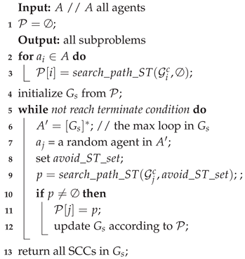
The decomposition based on break loops is presented in Algorithm 1. The algorithm proceeds as follows:
- Lines 1–4: initial dependency paths and ;
- Lines 5–12: break loops iteratively until a terminate condition is met;
- Lines 13–14: return all SCCs in as results of decomposition.
| Algorithm 1: Decomposition_of_MAPF_problems |
 |
4.2. Solving Subproblems and Combine Their Solution
In this section, we present our approach for solving subproblems independently with a solvability safeguard to handle unsolvable cases, and describe the merging process of all subproblem solutions to obtain a conflict-free global solution.
4.2.1. Solving Subproblems with Solvability Safeguard
In solving subproblems, they are processed sequentially while avoiding conflicts with both previous subproblems’ target states and subsequent subproblems’ start states. However, as previously mentioned, the solvability check condition may incorrectly classify unsolvable subproblems as solvable, potentially resulting in some unsolvable subproblems.
To preserve solvability, motivated by ID [11], we propose a solvability safeguard with four components:
- When detecting an unsolvable subproblem (failed to find a solution within a time limit, e.g., 60 seconds), we solve it while ignoring other subproblems’ agents (allowing conflicts with other agents’ start or target states). Since the original LA-MAPF subproblem is assumed solvable, part of it remains solvable.
- We verify whether the solution conflicts with: previous subproblems’ target states, or subsequent subproblems’ start states (the solution must satisfy at least one of: 1) conflict with a previous subproblem’s start state; 2) conflict with a subsequent subproblem’s target state, otherwise, it is solvable (if the raw problem is solvable) while avoiding conflicts with both previous subproblems’ target states and subsequent subproblems’ start states).
- We merge all subproblems between the affected previous and subsequent subproblems into a new subproblem to replace all merged subproblems, creating a new LA-MAPF subproblem decomposition.
- We attempt to solve the subproblems in this new decomposition.
After merging, all subproblems still pass the legality check. In the worst-case scenario, all subproblems may merge into a single problem - reverting to the original problem formulation. This guarantees that our solvability safeguard can always prevent loss of solvability.
4.2.2. Merge Solution
After solving all subproblems and obtaining their solutions, we merge them to construct a conflict-free global solution. As established in the simplified scenario, each subproblem’s solution avoids both: previous subproblems’ target states and subsequent subproblems’ start states. Thus, we can always guarantee a conflict-free solution by inserting wait actions at each subproblem’s solution until all agents from previous subproblems reach their targets. This approach ensures the solution is conflict-free in worst-case scenarios, though potentially at the cost of additional wait actions when agents could otherwise begin moving earlier without conflicts.
To optimize solution quality, we propose an improved merging method:
- Initialize at
- For each subproblem: 1) determine necessary wait actions at the current timestep to avoid conflicts with previous subproblems’ solutions; 2) track the maximum required wait duration
- Apply the maximum wait actions to all paths in the current subproblem to prevent: conflicts with prior solutions and intra-subproblem path conflicts
- , iterate until all solutions are conflict-free.
There are two types of MAPF methods.
- In the first type, the same joint state of all agents is allowed to occur more than once in a solution, as in EECBS.
- In the second type, the same joint state of all agents is not allowed to occur more than once, such as in LaCAM. More details on how LaCAM forbids the same configuration from occurring again can be found in its implementation1.
The first type is complete in terms of avoiding conflicts with external paths (i.e., paths of agents not included in the current subproblem). In contrast, the second type is not complete in this sense, because all agents may need to wait at their current states to avoid conflicts with external agents’ paths, but such waiting is forbidden.
We refer to the first type of MAPF methods as p-complete methods, and the second type as p-incomplete methods. When solving subproblems, p-complete MAPF methods can treat the paths of agents from other subproblems as constraints to be avoided. As a result, no additional wait actions are required during solution merging, since the subproblem solutions are already mutually conflict-free.
In contrast, p-incomplete MAPF methods cannot incorporate external paths as constraints. Therefore, adding wait actions during the merging of subproblem solutions is necessary to ensure a conflict-free global solution.
4.2.3. Implementation
In this section, we present the implementation details for solving subproblems and merging their solutions.
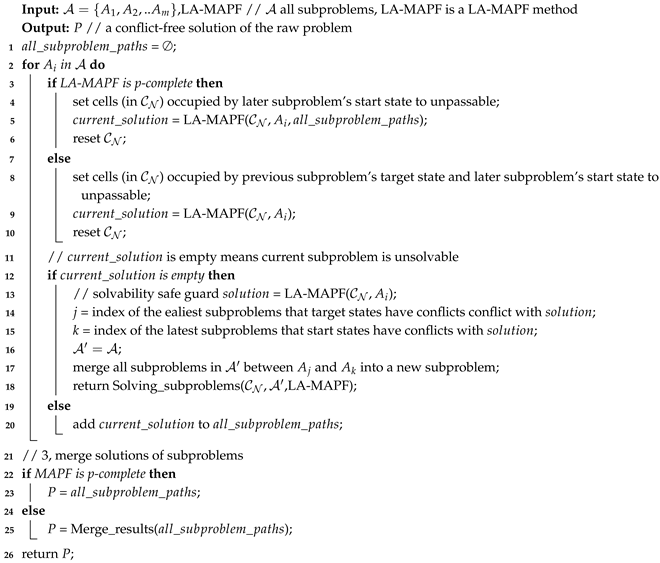
The subproblem-solving process with solvability safeguard is presented in Algorithm 2. The algorithm proceeds as follows:
- Lines 1–10: sequentially solve all subproblems
- Lines 11–18: apply the solvability safeguard by merging unsolvable subproblems with other subproblems and solving subproblems in the new decomposition
- Lines 19–20: stores solutions for the current subproblems
- Lines 21–25: merges subproblem solutions (skipped for p-complete methods, as their solutions inherently avoid conflicts with other subproblems’ solutions)
A toy example about the solvability safeguard is shown in Figure 15.
| Algorithm 2: Solving_subproblems |
 |
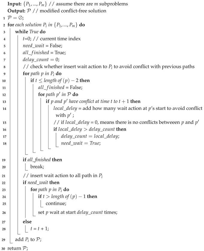
The merging algorithm proceeds through three key phases, as shown in Algorithm 3:
- Conflict Detection (Lines 1–13): 1) verifies whether the current subproblem’s path conflicts with previous subproblems’ solutions; 2) performs pairwise collision checks at each timestep
-
Wait Time Calculation (Lines 14–18):1) computes required wait durations when conflicts are detected;2) maintains the maximum necessary wait time across all conflicts;3) applies temporal padding to ensure safe separation
-
Solution Integration (Lines 19–30):
- –
- Path Modification (Lines 19–28): a) inserts calculated wait actions into unfinished paths; b) ensures all current subproblem paths are conflict-free
- –
- Solution Aggregation (Lines 29–30): a) incorporates modified solutions into the merged plan; b) returns the complete conflict-free solution after processing all subproblems
| Algorithm 3: Merge_solutions |
 |
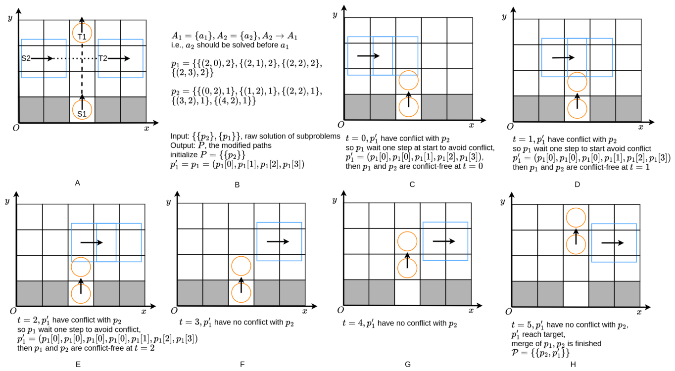
The merging process is illustrated in Figure 16, showing both the temporal adjustments and final coordinated solution.
Figure 16.
This figure shows a LA-MAPF problem containing two agents (Figure A) that belong to different subproblems and the subproblems’ solutions (Figure B), and how to merge them into a conflict-free solution (Figures C∼H).
Figure 16.
This figure shows a LA-MAPF problem containing two agents (Figure A) that belong to different subproblems and the subproblems’ solutions (Figure B), and how to merge them into a conflict-free solution (Figures C∼H).
4.3. Completeness and Suboptimality
Besides efficiency, our major focus, completeness and optimality are two important aspects in the evaluation of MAPF methods. Therefore, in this section, we discuss the completeness of MAPF methods under our problem decomposition, and the suboptimality of the resulting solutions.
4.3.1. Completeness
Although the solvability check may misjudge an unsolvable LA-MAPF problem as solvable, and may decompose a solvable problem into unsolvable subproblems, we introduce a solvability safeguard to ensure all subproblems are solvable. In the worst case, all subproblems are merged back into the original problem and solved by the MAPF method that the framework uses. Therefore, if a complete MAPF method is combined with our MAPF problem decomposition, the resulting approach remains complete.
4.3.2. Suboptimality
In this section, we discuss the suboptimality of the merged solution in the worst case. In summary, since we need to add wait actions when merging solutions of subproblems, the solution produced by our framework is unboundedly suboptimal in the worst case (an example of a bounded-suboptimal MAPF method is EECBS [21]). We analyze both the makespan and the sum of costs in the worst case. The proof consists of two steps: we first discuss how many wait actions each subproblem solution needs to add, and then analyze how many wait actions are introduced in the merged solution.
As the merging solution needs to add wait actions so that the solution is conflict-free, decomposition of the MAPF problem affects the solution quality. Here, we analyze how the decomposition of a MAPF problem affects the makespan and the sum of costs in the best and worst cases.
In the best case, when paths of different subproblems have no conflicts, no wait actions are needed, so decomposition has no side effects. According to empirical evidence, this situation usually arises when the agents are sparsely distributed.
However, when the agents are densely distributed, the merging solution may need to add many wait actions. For quantitative analysis, we assume that a LA-MAPF problem has k agents and n subproblems . We denote the makespan and the sum of costs of subproblem after merging as and . The makespan and sum of costs of the total solution before merging are M and S, respectively, and those after merging are and , respectively. In the worst case, each subproblem’s solution needs waiting actions that are equal to the maximum makespan of the previous subproblems’ solutions (i.e., waiting until all previous subproblems’ agents have reached their targets), because all previous agents remain at their target states.
In the worst case, the last subproblem has the largest makespan, as it needs to wait until the agents of all previous subproblems reach their targets.
In the worst case, the increase in every subproblem’s solution is the product of the current subproblem’s size and the sum of the sizes of all previous subproblems.
Denote .
The first subproblem has the smallest makespan in the worst case, so . As the first subproblem’s solution does not need to wait, .
Denote .
and reflect how much worse the merged solution can be; the larger these values are, the worse the solution. These two values depend on multiple factors, such as the number of subproblems, the minimum makespan of the subproblem solutions, and the minimum subproblem size; therefore, they have no finite upper bound. Therefore, in the worst case, the merging process may produce a suboptimal and unbounded solution, even when an optimal LA-MAPF solver such as LA-CBS is used.
5. Results
In this section, we evaluate the performance of our framework, Break Loops (BL), on both MAPF and LA-MAPF problems. We compare BL with Independence Detection (ID), our previous bipartition-based decomposition method (BP), and the raw MAPF methods. The comparison metrics include time cost, success rate, makespan, and sum of costs to assess overall performance. We also conduct an ablation study to examine how each component contributes to Break Loops. As Break Loops contains two phases: (1) initialization of subproblems and (2) iteratively breaking loops to obtain smaller subproblems, we add Break Loops initialization (BI) to the evaluation.
Additionally, we compare max subproblem size, number of subproblems, and decomposition time cost to evaluate the decomposition approaches (BL, BP, and ID). Specifically, since ID does not separate the process into two distinct phases—decomposition followed by planning—as BL and BP do, only the decomposition time costs of BL and BP are compared.
As a common practice in solving MAPF problems, we set an upper bound of 60 seconds on the time cost. Methods that are complete but fail to find a solution within the given time limit are considered failures.
To ensure a fair comparison on solution quality, we only consider cases in which both methods are successful.
So, we compared the solution quality of methods pair by pair, such as raw CBS and CBS with ID, LaCAM with BP, and LaCAM with BL.
We select 10 maps from the classic MAPF benchmark dataset2 [22,23] as test environments. To evaluate how problem decomposition scales with the number of agents, we vary the number of agents from 10 to 1000 (or the maximum number allowed by the map, as some smaller maps may not support 1000 agents). For each agent count, 100 random instances are generated.
Since MAPF is essentially a simplified version of LA-MAPF, our framework can also be applied to MAPF problems. Therefore, we evaluate its performance on both MAPF and LA-MAPF instances.
For LA-MAPF problems, to the best of our knowledge, no public dataset is currently available. Hence, we randomly generate LA-MAPF problems for experimentation. These problems include two types of agents: circular agents and rectangular agents, each with randomly assigned sizes. The radii of the circular agents range from 0.4 to 2.0 cells, while the widths and lengths of the rectangular agents range from 0.4 to 4.0 cells. An example of a map and a corresponding LA-MAPF problem is shown in Figure 17.
For the MAPF methods, we apply CBS and LaCAM. CBS is an optimal MAPF algorithm, while LaCAM is one of the fastest MAPF methods currently available. For experiments on LA-MAPF, we extend CBS and LaCAM to LA-CBS (CBS for large agents) and LA-LaCAM, following the implementation guidelines in [8]. Below, we provide a brief introduction to both CBS and LaCAM.
Conflict-Based Search (CBS) [1] stands out as one of the most well-known MAPF methods. It is characterized by its completeness and optimality. CBS is a two-level algorithm. At the high level, a search is performed on a tree based on conflicts between agents. At the low level, a search is performed for a single agent at a time. The algorithm updates each agent’s path in isolation at the low level while avoiding all constraints set by the high-level tree. The algorithm exits when it finds a conflict-free solution or all nodes in the high-level tree have been expanded and no new nodes are available. We apply CBS with mutex propagation for comparison [12].
LaCAM [4] is a complete but suboptimal two-level MAPF method. At the high level, it explores a sequence of configurations, where each search node corresponds to a specific configuration. A configuration represents the current locations of all agents. At the low level, LaCAM searches for constraints that determine where each agent should move in the next configuration. If successful, the resulting configuration is added to the high-level search. If no new configurations can be generated, the algorithm terminates with failure.
LaCAM is p-incomplete, as it updates the states of all agents simultaneously at each step. Its implementation forbids repeated configurations, which limits its ability to resolve conflicts with external paths in the same way as CBS. Consequently, we only evaluate Independence Detection (ID) in combination with CBS, and do not test ID with LaCAM.
Given the large number of figures used to present the results, we summarize the key findings in tables placed in the main body of the paper. Details of how the performance of different methods varies with the number of agents are provided in the Appendix.
All experiments were conducted on a computer running Ubuntu 20.04, equipped with a 2.5 GHz CPU and 128 GB of RAM. All implementations were written in C++.
5.1. Application on MAPF
5.1.1. CBS
In this section, we focus on the comparison between raw CBS and CBS enhanced with our Break Loops (BL) framework. A summary of the results is presented in Table 1, Table 2 and Table 3, while detailed results are illustrated in Figure A1 and Figure A2.
As shown in these tables and figures, raw CBS becomes increasingly time-consuming as the number of agents increases, leading to a lower success rate. In contrast, CBS with BL significantly reduces the time cost and achieves a higher success rate, as expected. Some results are shown in Figure 18. However, CBS with problem decomposition yields suboptimal solutions. This is because merging the solutions of subproblems often requires inserting wait actions to ensure global consistency, whereas CBS is an optimal solver when applied directly.
5.1.2. LaCAM
In this section, we focus on the comparison between raw LaCAM and LaCAM combined with the Break Loops (BL) framework. A summary of the results is presented in Table 4, Table 5 and Table 6, while detailed results are illustrated in Figure A3 and Figure A4
As shown in these tables and figures, raw LaCAM is highly efficient on most maps, and the time cost of problem decomposition using BL is comparable to that of raw LaCAM. Therefore, BL provides little benefit in these cases. However, on maps where LaCAM incurs higher time costs than the decomposition overhead (e.g., (1) warehouse-10-20-10-2-1 and (2) warehouse-20-40-10-2-1), BL effectively reduces the total time cost and improves the success rate. Some results are shown in Figure 19.
Similar to CBS, LaCAM with problem decomposition produces lower-quality solutions. This is because merging subproblem solutions requires inserting additional wait actions to ensure a conflict-free global solution.
5.2. Application on LA-MAPF
5.2.1. LA-CBS
In this section, we focus on the comparison between raw LA-CBS and LA-CBS enhanced with the Break Loops (BL) framework. A summary of the results is presented in Table 7, Table 8 and Table 9, while detailed results are illustrated in Figure A5 and Figure A6.
As shown in these tables and figures, similar to CBS, raw LA-CBS is time-consuming and thus exhibits a lower success rate as the number of agents increases. In contrast, LA-CBS with BL significantly reduces the time cost and achieves a higher success rate. Some results are shown in Figure 20. However, LA-CBS with problem decomposition yields lower-quality solutions. This is because merging subproblem solutions often requires adding wait actions to ensure a conflict-free overall plan, and raw LA-CBS is an optimal method.
5.2.2. LA-LaCAM
In this section, we focus on the comparison between raw LA-LaCAM and LA-LaCAM with the Break Loops (BL) framework. A summary of the results is presented in Table 10, Table 11 and Table 12, while detailed results are illustrated in Figure A7 and Figure A8.
As shown in these tables and figures, unlike LaCAM, LA-LaCAM is more time-consuming due to the overhead of conflict detection between large agents. As the number of agents increases, its success rate decreases accordingly. In this case, applying BL significantly reduces the time cost of LA-LaCAM, leading to a higher success rate. Some results are shown in Figure 21. However, similar to previous observations, LA-LaCAM with problem decomposition produces lower-quality solutions. This is because merging subproblem solutions often requires inserting wait actions to ensure a conflict-free final plan.
5.3. Comparison between ID, BP and BL
In this section, we focus on the comparison between raw LA-LaCAM and LA-LaCAM with the Break Loops (BL) framework. A summary of the results is presented in Table 1, Table 4, Table 7, and Table 10, while detailed results are shown in Figure A1, Figure A2, Figure A3, Figure A4, Figure A5, Figure A6, Figure A7 and Figure A8.
In terms of time cost, ID incurs a higher time cost compared to BL and BP, and it also exhibits a lower success rate. The main reasons are as follows:
- ID does not consider the order in which subproblems are solved, whereas both BP and BL do. Consequently, the layered decomposition used in BL is more likely to divide a MAPF problem into smaller and more manageable subproblems.
- When ID attempts to verify whether a group (i.e., a subproblem) can avoid conflicts with another group, it does not prevent previously resolved conflicts from occurring again between the two groups. As a result, ID may fall into infinite loops. For example, suppose Group A is modified to avoid conflicts with Group B. Later, a conflict between Group A and Group C is detected, prompting ID to update Group A’s solution to avoid Group C. However, this new solution may reintroduce conflicts with Group B. ID will then repeat the process of resolving conflicts with Groups B and C, potentially leading to a loop that continues until the time limit is reached. This issue is rare when agents are sparse but becomes frequent in densely populated scenarios.
- In BL and BP, each agent is involved in the multi-agent pathfinding process only once. In contrast, in ID, an agent may participate multiple times, as it can be merged into different groups at various stages. This repeated involvement increases the overall time cost of ID compared to BP and BL.
Compared to BP, BL has a lower decomposition time cost, smaller maximum subproblem size, and a larger number of subproblems. As a result, MAPF with BL requires less overall computation time and achieves a higher success rate. This improvement is mainly due to two factors: (1) BP considers only the agents within the current subproblem during decomposition, while BL takes all agents into account; and (2) BL explicitly aims to minimize the size of the largest subproblem at every step, whereas BP does not. These differences enable BL to produce a better decomposition more efficiently.
5.4. Ablation Study
To evaluate the contribution of each component in our framework, we conduct an ablation study, which compares Break Loops with only initialization (BI) and Break Loops (BI) in the experiments. The related results can be found in Table 1, Table 4, Table 7, and Table 10 and Figure A1, Figure A2, Figure A3, Figure A4, Figure A5, Figure A6, Figure A7 and Figure A8.
As shown in the above results, on maps with sparse agents (e.g., MAPF: Berlin_1_256 and Boston_0_256; LA-MAPF: Berlin_1_256 and Boston_2_256), BI can decompose the original problem into very small subproblems, so there is no significant difference between the performance of BI and BL, as shown in Figure 22 and Figure 23. However, on maps with dense agents (e.g., MAPF: empty-32-32 and random-32-32-20; LA-MAPF: empty-32-32 and empty-48-48), BL uses the optimization technique to decompose the original problem into much smaller subproblems, thereby reducing the time cost and increasing the success rate. In summary, compared to BI, BL has a smaller time cost and a higher success rate on average. The initialization of BL plays a major role on maps with sparse agents, while the optimization technique plays a major role on maps with dense obstacles.
5.5. Summary
In summary, our framework significantly reduces the time cost and improves the success rate of CBS, LA-CBS, and LA-LaCAM. For LaCAM, BL does not improve performance when its time cost is close to the decomposition time cost. However, BL can still enhance LaCAM’s performance when LaCAM requires more time than BL’s decomposition process. Our framework also demonstrates significant advantages over our previous method BP and over Independence Detection (ID), including smaller maximum subproblem sizes, a larger number of subproblems, lower time cost, and higher success rates. Nevertheless, the effectiveness of BL, BP, and ID decreases as the number of agents increases.
6. Conclusions and Discussion
Since each agent occupies multiple cells, solving LA-MAPF (Large-Agent Multi-Agent Path Finding) becomes increasingly time-consuming as the number of agents grows. Motivated by the exponential increase in computational cost with the number of agents, we propose Break Loops, a divide-and-conquer framework for accelerating MAPF algorithms.
Our method employs neighborhood search to iteratively reduce the size of the largest subproblem until a time or iteration limit is reached. Each resulting subproblem is then solved independently, ensuring that agents avoid the target states of earlier subproblems and the start states of later ones. To guarantee solvability, we introduce a safeguard mechanism: when an unsolvable subproblem is detected, it is merged with others until all subproblems become solvable. Finally, the solutions to all subproblems are combined into a conflict-free solution of the original problem.
The experimental results demonstrate that our framework is highly effective for solving LA-MAPF problems. Compared to raw LA-MAPF methods, applying our framework significantly reduces time cost and improves success rate. Furthermore, Break Loops outperforms both Independence Detection and our previous decomposition-based approach. Although our framework can also be applied to classic MAPF problems, it may not yield substantial time savings when the underlying MAPF method is already highly efficient (e.g., LaCAM).
Despite its benefits, Break Loops has limitations: its effectiveness diminishes as the number of agents increases. Nevertheless, even in the worst case—when the problem cannot be decomposed into smaller subproblems—its performance is never worse than that of the raw LA-MAPF methods.
In future work, we plan to apply LA-MAPF decomposition to real-world scenarios, thereby extending our framework to practical applications. We will also focus on optimizing the decomposition process, as there is still room for improvement— for example, by solving multiple subproblems concurrently on parallel threads.
7. Reproducibility Checklist for JAIR
Select the answers that apply to your research – one per item.
All Articles:
- All claims investigated in this work are clearly stated. [yes]
- Clear explanations are given how the work reported substantiates the claims. [yes]
- Limitations or technical assumptions are stated clearly and explicitly. [yes]
- Conceptual outlines and/or pseudo-code descriptions of the AI methods introduced in this work are provided, and important implementation details are discussed. [yes]
- Motivation is provided for all design choices, including algorithms, implementation choices, parameters, data sets and experimental protocols beyond metrics. [yes]
Articles Containing Theoretical Contributions:
Does this paper make theoretical contributions? [yes/no]
If yes, please complete the list below.
- All assumptions and restrictions are stated clearly and formally. [yes]
- All novel claims are stated formally (e.g., in theorem statements). [yes]
- Proofs of all non-trivial claims are provided in sufficient detail to permit verification by readers with a reasonable degree of expertise (e.g., that expected from a PhD candidate in the same area of AI). [yes]
- Complex formalism, such as definitions or proofs, is motivated and explained clearly. [yes]
- The use of mathematical notation and formalism serves the purpose of enhancing clarity and precision; gratuitous use of mathematical formalism (i.e., use that does not enhance clarity or precision) is avoided. [yes]
- Appropriate citations are given for all non-trivial theoretical tools and techniques. [yes]
Articles Reporting on Computational Experiments:
Does this paper include computational experiments? [yes]
If yes, please complete the list below.
- All source code required for conducting experiments is included in an online appendix or will be made publicly available upon publication of the paper. The online appendix follows best practices for source code readability and documentation as well as for long-term accessibility. [yes]
- The source code comes with a license that allows free usage for reproducibility purposes. [yes]
- The source code comes with a license that allows free usage for research purposes in general. [yes]
- Raw, unaggregated data from all experiments is included in an online appendix or will be made publicly available upon publication of the paper. The online appendix follows best practices for long-term accessibility. [yes]
- The unaggregated data comes with a license that allows free usage for reproducibility purposes. [yes]
- The unaggregated data comes with a license that allows free usage for research purposes in general. [yes]
- If an algorithm depends on randomness, then the method used for generating random numbers and for setting seeds is described in a way sufficient to allow replication of results. [yes]
- The execution environment for experiments, the computing infrastructure (hardware and software) used for running them, is described, including GPU/CPU makes and models; amount of memory (cache and RAM); make and version of operating system; names and versions of relevant software libraries and frameworks. [yes]
- The evaluation metrics used in experiments are clearly explained and their choice is explicitly motivated. [yes]
- The number of algorithm runs used to compute each result is reported. [yes]
- Reported results have not been “cherry-picked” by silently ignoring unsuccessful or unsatisfactory experiments. [yes]
- Analysis of results goes beyond single-dimensional summaries of performance (e.g., average, median) to include measures of variation, confidence, or other distributional information. [yes]
- All (hyper-) parameter settings for the algorithms/methods used in experiments have been reported, along with the rationale or method for determining them. [yes]
- The number and range of (hyper-) parameter settings explored prior to conducting final experiments have been indicated, along with the effort spent on (hyper-) parameter optimisation. [yes]
- Appropriately chosen statistical hypothesis tests are used to establish statistical significance in the presence of noise effects. [yes]
Articles Using Data Sets:
Does this work rely on one or more data sets (possibly obtained from a benchmark generator or similar software artifact)? [yes]
If yes, please complete the list below.
- All newly introduced data sets are included in an online appendix or will be made publicly available upon publication of the paper. The online appendix follows best practices for long-term accessibility with a license that allows free usage for research purposes. [yes]
- The newly introduced data set comes with a license that allows free usage for reproducibility purposes. [yes]
- The newly introduced data set comes with a license that allows free usage for research purposes in general. [yes]
- All data sets drawn from the literature or other public sources (potentially including authors’ own previously published work) are accompanied by appropriate citations. [yes]
- All data sets drawn from the existing literature (potentially including authors’ own previously published work) are publicly available. [yes]
- All new data sets and data sets that are not publicly available are described in detail, including relevant statistics, the data collection process and annotation process if relevant. [yes]
- All methods used for preprocessing, augmenting, batching or splitting data sets (e.g., in the context of hold-out or cross-validation) are described in detail. [yes]
Appendix A. Results
Figure A1.
These figures illustrate the performance of raw CBS, CBS with BP, BL, and ID across various maps. The performance of these methods is evaluated in terms of time costs, success rate, makespan, sum of cost, max subproblem size, number of subproblems, and time cost of decomposition. Additionally, we provide information on the scale and the number of passable cells (in brackets).
Figure A1.
These figures illustrate the performance of raw CBS, CBS with BP, BL, and ID across various maps. The performance of these methods is evaluated in terms of time costs, success rate, makespan, sum of cost, max subproblem size, number of subproblems, and time cost of decomposition. Additionally, we provide information on the scale and the number of passable cells (in brackets).
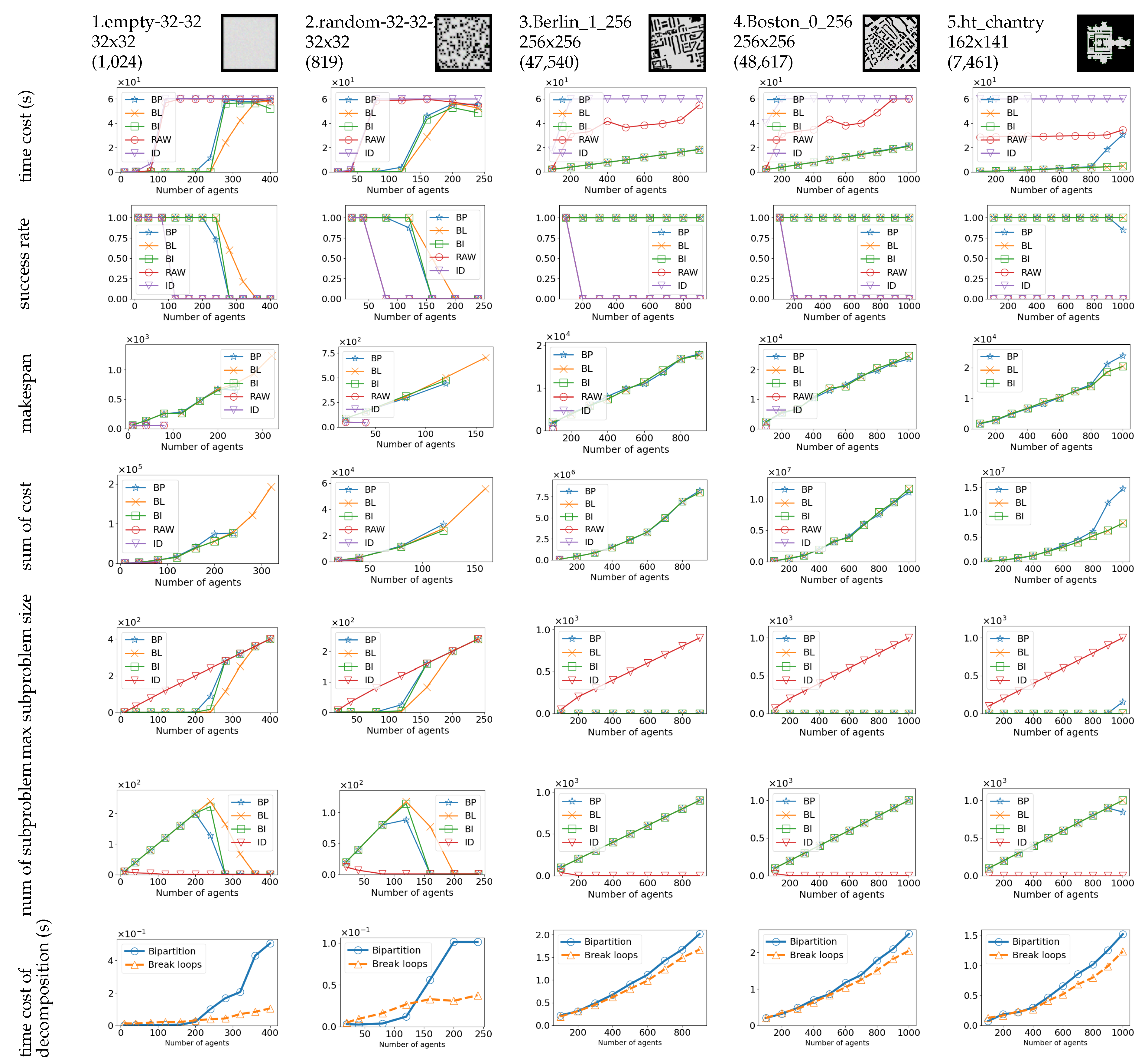
Figure A2.
These figures illustrate the performance of raw CBS, CBS with BP, BL, and ID across various maps. The performance of these methods is evaluated in terms of time cost, success rate, makespan, sum of costs, max subproblem size, number of subproblems, and time cost of decomposition. Additionally, we provide information on the scale and the number of passable cells (in brackets).
Figure A2.
These figures illustrate the performance of raw CBS, CBS with BP, BL, and ID across various maps. The performance of these methods is evaluated in terms of time cost, success rate, makespan, sum of costs, max subproblem size, number of subproblems, and time cost of decomposition. Additionally, we provide information on the scale and the number of passable cells (in brackets).
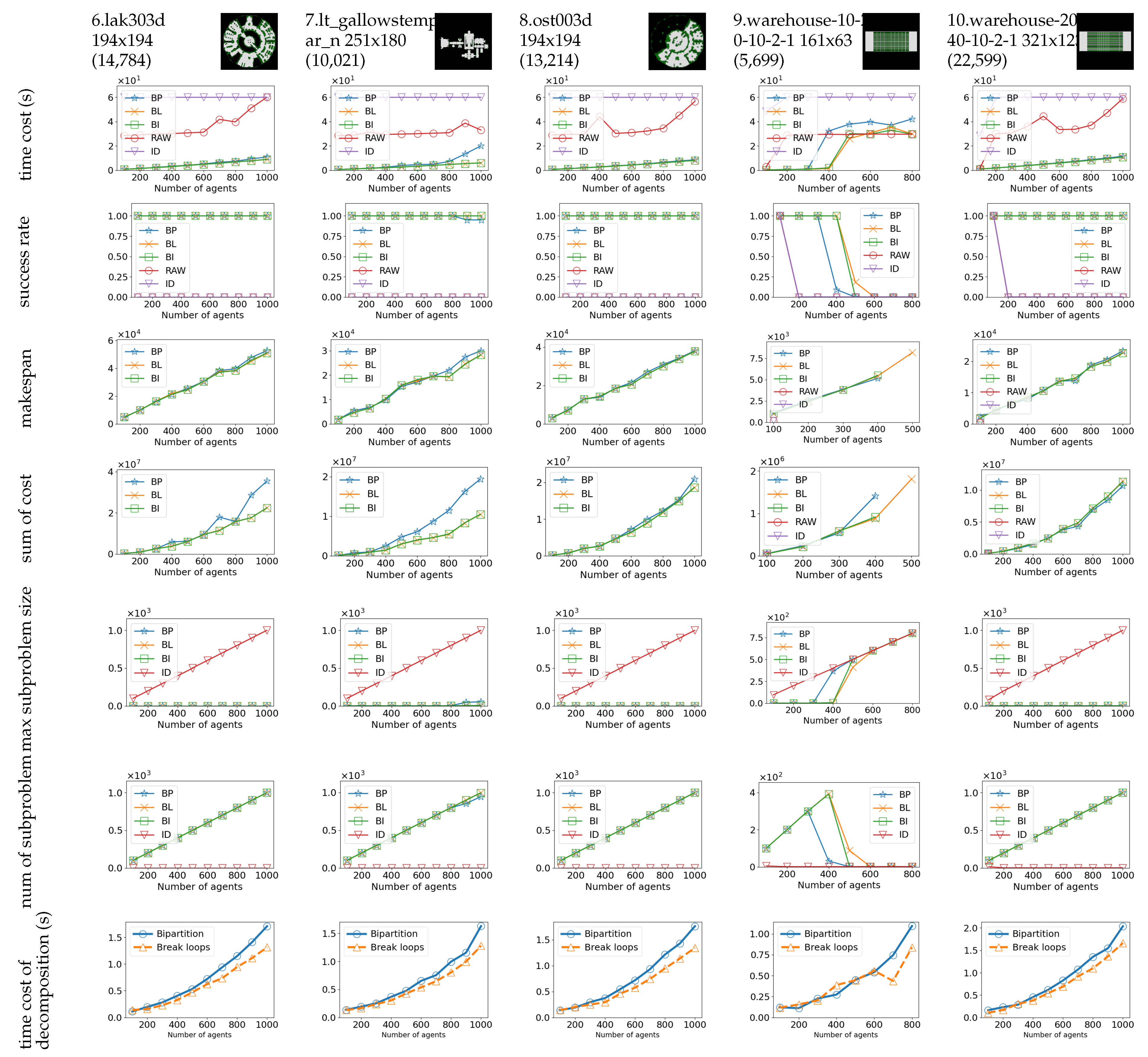
Figure A3.
These figures illustrate the performance of raw LaCAM and LaCAM with BP, BL across various maps. The performance of these methods is evaluated in terms of time cost, success rate, makespan, sum of costs, max subproblem size, number of subproblems, and time cost of decomposition. Additionally, we provide information on the scale and the number of passable cells (in brackets).
Figure A3.
These figures illustrate the performance of raw LaCAM and LaCAM with BP, BL across various maps. The performance of these methods is evaluated in terms of time cost, success rate, makespan, sum of costs, max subproblem size, number of subproblems, and time cost of decomposition. Additionally, we provide information on the scale and the number of passable cells (in brackets).
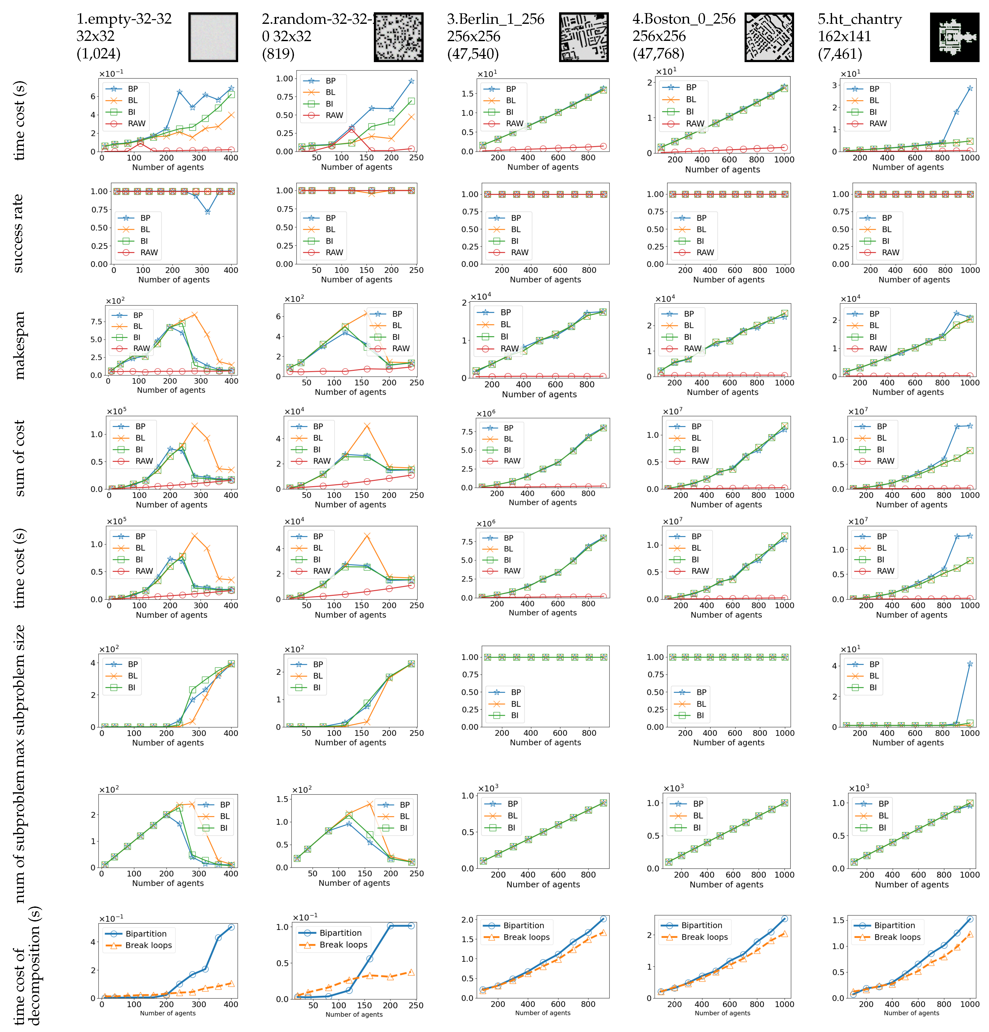
Figure A4.
These figures illustrate the performance of raw LaCAM and LaCAM with BP, BL across various maps. The performance of these methods is evaluated in terms of time cost, success rate, makespan, sum of costs, max subproblem size, number of subproblems, and time cost of decomposition. Additionally, we provide information on the scale and the number of passable cells (in brackets).
Figure A4.
These figures illustrate the performance of raw LaCAM and LaCAM with BP, BL across various maps. The performance of these methods is evaluated in terms of time cost, success rate, makespan, sum of costs, max subproblem size, number of subproblems, and time cost of decomposition. Additionally, we provide information on the scale and the number of passable cells (in brackets).
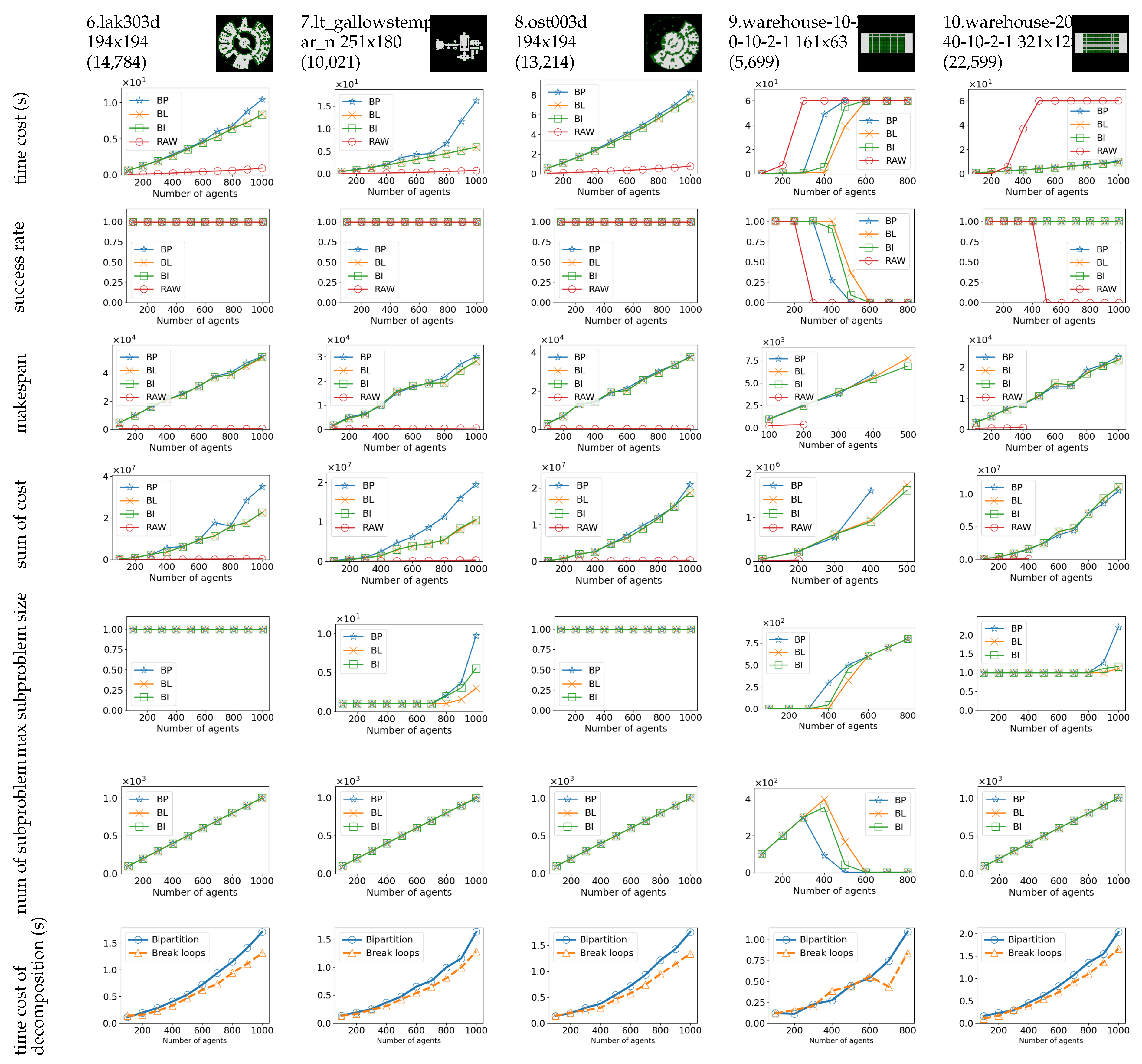
Figure A5.
These figures illustrate the performance of raw LA-CBS, LA-CBS with BP and BL, and ID across various maps. The performance of these methods is evaluated in terms of time cost, success rate, makespan, sum of costs, max subproblem size, number of subproblems, and time cost of decomposition. Additionally, we provide information on the scale and the number of free cells (in brackets).
Figure A5.
These figures illustrate the performance of raw LA-CBS, LA-CBS with BP and BL, and ID across various maps. The performance of these methods is evaluated in terms of time cost, success rate, makespan, sum of costs, max subproblem size, number of subproblems, and time cost of decomposition. Additionally, we provide information on the scale and the number of free cells (in brackets).
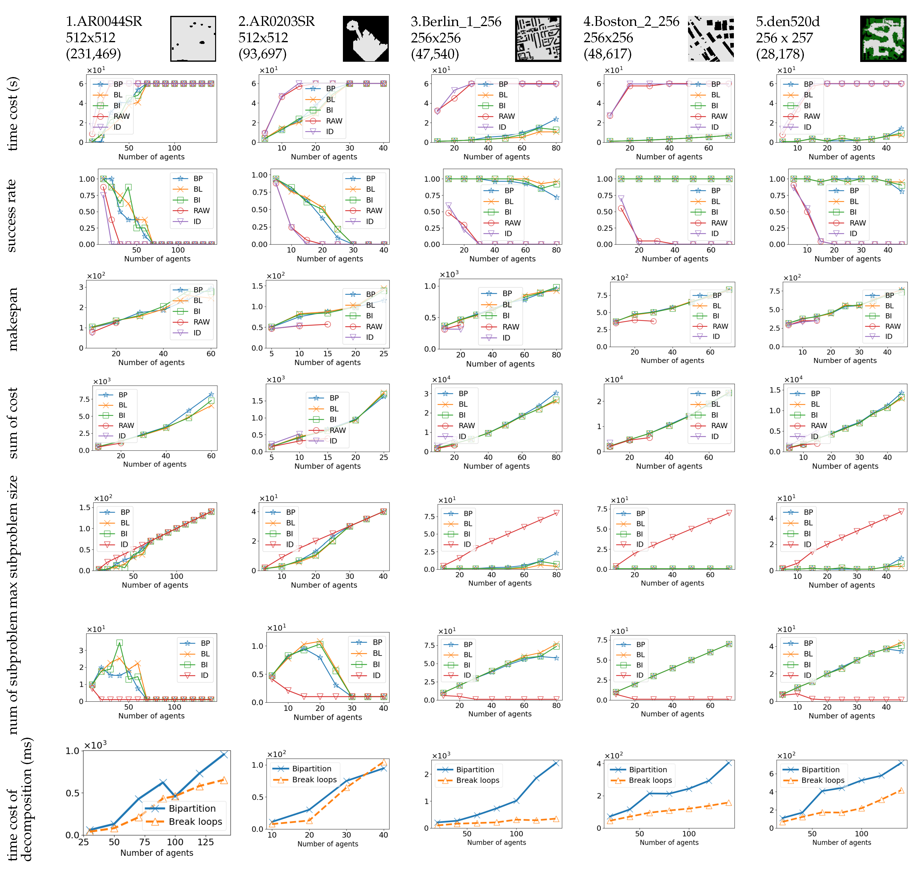
Figure A6.
These figures illustrate the performance of raw LA-CBS, LA-CBS with BP, and BL, and ID across various maps. The performance of these methods is evaluated in terms of time cost, success rate, makespan, sum of costs, max subproblem size, number of subproblems, and time cost of decomposition. Additionally, we provide information on the scale and the number of free cells (in brackets).
Figure A6.
These figures illustrate the performance of raw LA-CBS, LA-CBS with BP, and BL, and ID across various maps. The performance of these methods is evaluated in terms of time cost, success rate, makespan, sum of costs, max subproblem size, number of subproblems, and time cost of decomposition. Additionally, we provide information on the scale and the number of free cells (in brackets).
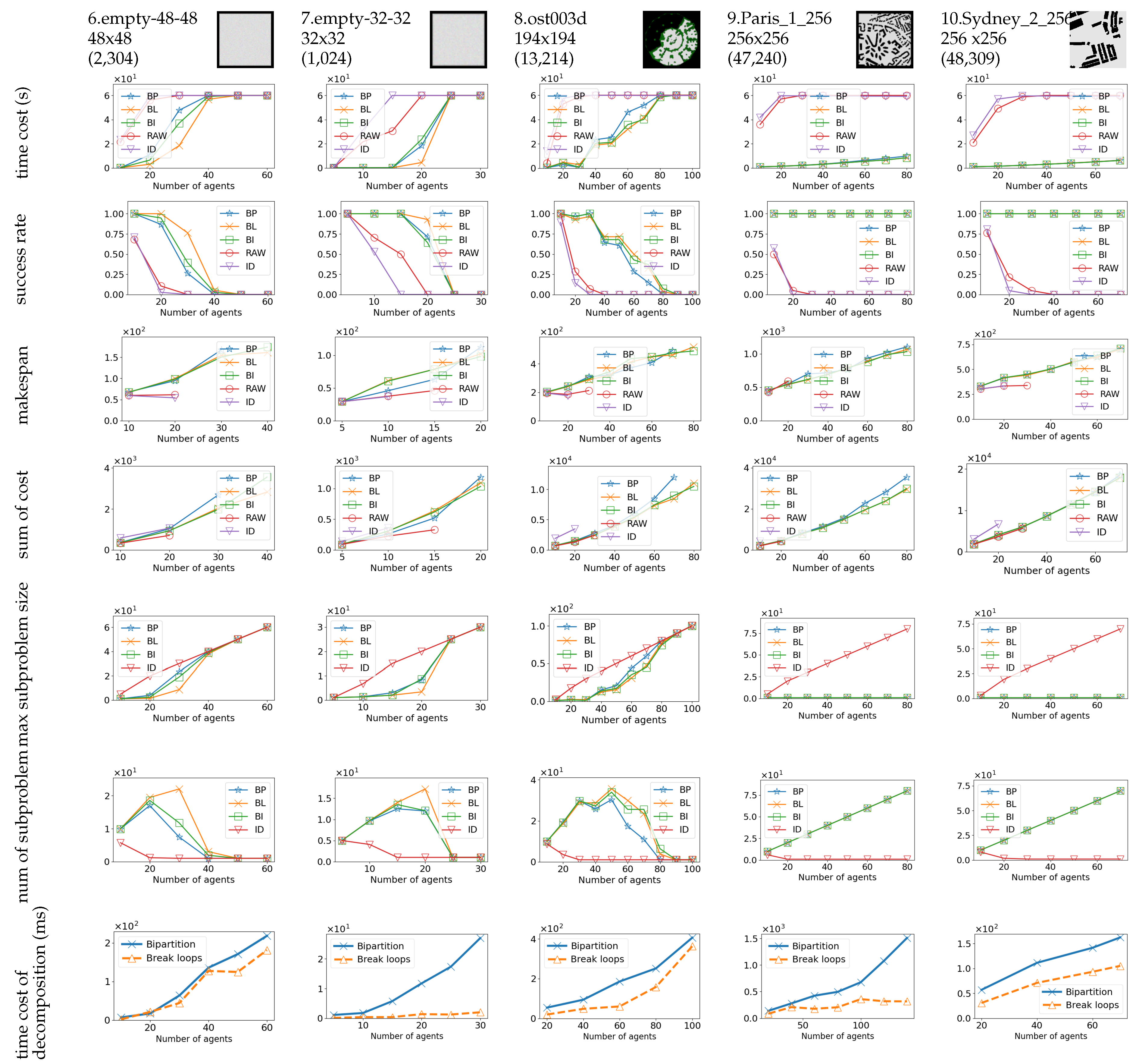
Figure A7.
These figures illustrate the performance of raw LA-LaCAM and LA-LaCAM with BP, and BL across various maps. The performance of these methods is evaluated in terms of time cost, success rate, makespan, sum of costs, max subproblem size, number of subproblems, and time cost of decomposition. Additionally, we provide information on the scale and the number of passable cells (in brackets).
Figure A7.
These figures illustrate the performance of raw LA-LaCAM and LA-LaCAM with BP, and BL across various maps. The performance of these methods is evaluated in terms of time cost, success rate, makespan, sum of costs, max subproblem size, number of subproblems, and time cost of decomposition. Additionally, we provide information on the scale and the number of passable cells (in brackets).
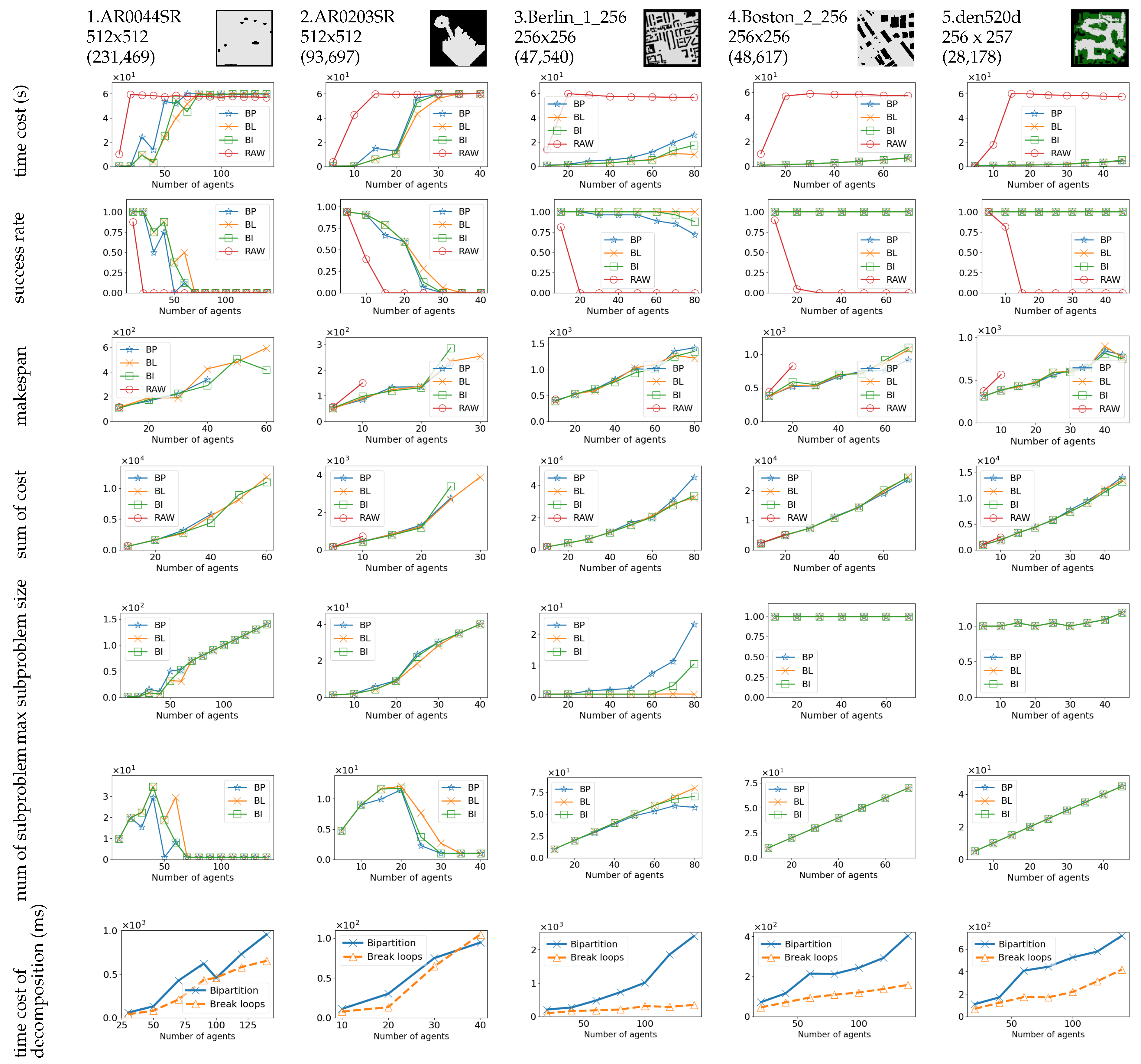
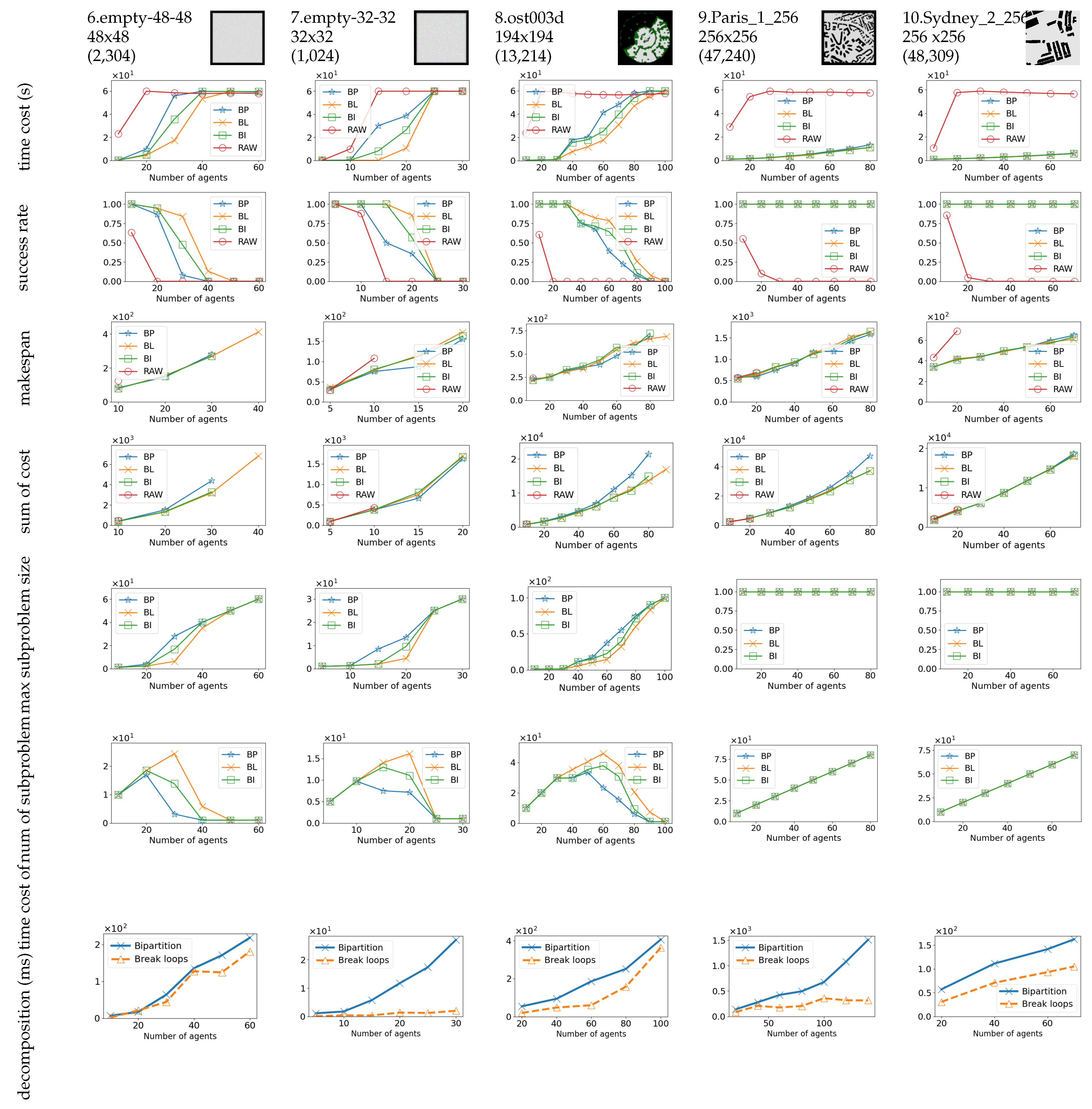
Figure A8.
These figures illustrate the performance of raw LA-LaCAM and LA-LaCAM with BP, BL across various maps. The performance of these methods is evaluated in terms of time cost, success rate, makespan, sum of costs, max subproblem size, number of subproblems, and time cost of decomposition. Additionally, we provide information on the scale and the number of passable cells (in brackets).
Figure A8.
These figures illustrate the performance of raw LA-LaCAM and LA-LaCAM with BP, BL across various maps. The performance of these methods is evaluated in terms of time cost, success rate, makespan, sum of costs, max subproblem size, number of subproblems, and time cost of decomposition. Additionally, we provide information on the scale and the number of passable cells (in brackets).
References
- Sharon, G.; Stern, R.; Felner, A.; Sturtevant, N.R. Conflict-based search for optimal multi-agent pathfinding. Artificial intelligence 2015, 219, 40–66. [CrossRef]
- Ma, H.; Harabor, D.; Stuckey, P.J.; Li, J.; Koenig, S. Searching with consistent prioritization for multi-agent path finding. In Proceedings of the Proceedings of the AAAI conference on artificial intelligence, 2019, Vol. 33, pp. 7643–7650. [CrossRef]
- Okumura, K.; Machida, M.; Défago, X.; Tamura, Y. Priority Inheritance with Backtracking for Iterative Multi-agent Path Finding. In Proceedings of the Proceedings of the Twenty-Eighth International Joint Conference on Artificial Intelligence, IJCAI-19. International Joint Conferences on Artificial Intelligence Organization, 7 2019, pp. 535–542. [CrossRef]
- Okumura, K. Lacam: Search-based algorithm for quick multi-agent pathfinding. In Proceedings of the Proceedings of the AAAI Conference on Artificial Intelligence, 2023, Vol. 37, pp. 11655–11662. [CrossRef]
- Hönig, W.; Kiesel, S.; Tinka, A.; Durham, J.W.; Ayanian, N. Persistent and Robust Execution of MAPF Schedules in Warehouses. IEEE Robotics and Automation Letters 2019, 4, 1125–1131. [CrossRef]
- Liu, Z.; Wang, H.; Wei, H.; Liu, M.; Liu, Y.H. Prediction, Planning, and Coordination of Thousand-Warehousing-Robot Networks With Motion and Communication Uncertainties. IEEE Transactions on Automation Science and Engineering 2021, 18, 1705–1717. [CrossRef]
- Mavrogiannis, C.; Knepper, R.A. Multi-agent path topology in support of socially competent navigation planning. The International Journal of Robotics Research 2018, 38, 338 – 356. [CrossRef]
- Li, J.; Surynek, P.; Felner, A.; Ma, H.; Kumar, T.K.S.; Koenig, S. Multi-Agent Path Finding for Large Agents. In Proceedings of the Symposium on Combinatorial Search, 2019.
- Li, J.; Chen, Z.; Harabor, D.; Stuckey, P.J.; Koenig, S. MAPF-LNS2: Fast repairing for multi-agent path finding via large neighborhood search. In Proceedings of the Proceedings of the AAAI Conference on Artificial Intelligence, 2022, Vol. 36, pp. 10256–10265. [CrossRef]
- Yao, Z. LayeredMAPF: A Decomposition of Mapf Instance to Reduce Solving Costs. Preprints 2025. [CrossRef]
- Surynek, P.; Švancara, J.; Felner, A.; Boyarski, E. Variants of independence detection in sat-based optimal multi-agent path finding. In Proceedings of the Agents and Artificial Intelligence: 9th International Conference, ICAART 2017, Porto, Portugal, February 24–26, 2017, Revised Selected Papers 9. Springer, 2018, pp. 116–136.
- Zhang, H.; Li, Y.; Li, J.; Kumar, T.K.S.; Koenig, S. Mutex Propagation in Multi-Agent Path Finding for Large Agents. In Proceedings of the Symposium on Combinatorial Search, 2022.
- Wen, L.; Liu, Y.; Li, H. CL-MAPF: Multi-Agent Path Finding for Car-Like robots with kinematic and spatiotemporal constraints. Robotics and Autonomous Systems 2022, 150, 103997. [CrossRef]
- Bai, Y.; Kotpalliwar, S.; Kanellakis, C.; Nikolakopoulos, G. Multi-agent Path Planning Based on Conflict-Based Search (CBS) Variations for Heterogeneous Robots. Journal of Intelligent & Robotic Systems 2025, 111. [CrossRef]
- Standley, T.S. Finding Optimal Solutions to Cooperative Pathfinding Problems. Proceedings of the AAAI Conference on Artificial Intelligence 2010.
- Standley, T.S.; Korf, R.E. Complete Algorithms for Cooperative Pathfinding Problems. In Proceedings of the International Joint Conference on Artificial Intelligence, 2011.
- Sharon, G.; Stern, R.; Felner, A.; Sturtevant, N.R. Meta-Agent Conflict-Based Search For Optimal Multi-Agent Path Finding. In Proceedings of the Symposium on Combinatorial Search, 2021.
- Erdmann, M.; Lozano-Perez, T. On multiple moving objects. In Proceedings of the Proceedings. 1986 IEEE International Conference on Robotics and Automation, 1986, Vol. 3, pp. 1419–1424. [CrossRef]
- Čáp, M.; Novák, P.; Kleiner, A.; Selecký, M. Prioritized Planning Algorithms for Trajectory Coordination of Multiple Mobile Robots. IEEE Transactions on Automation Science and Engineering 2015, 12, 835–849. [CrossRef]
- Tarjan, R. Depth-first search and linear graph algorithms. SIAM journal on computing 1972, 1, 146–160. [CrossRef]
- Li, J.; Ruml, W.; Koenig, S. Eecbs: A bounded-suboptimal search for multi-agent path finding. In Proceedings of the Proceedings of the AAAI conference on artificial intelligence, 2021, Vol. 35, pp. 12353–12362. [CrossRef]
- Sturtevant, N. Benchmarks for Grid-Based Pathfinding. Transactions on Computational Intelligence and AI in Games 2012, 4, 144 – 148. [CrossRef]
- Stern, R.; Sturtevant, N.R.; Felner, A.; Koenig, S.; Ma, H.; Walker, T.T.; Li, J.; Atzmon, D.; Cohen, L.; Kumar, T.K.S.; et al. Multi-Agent Pathfinding: Definitions, Variants, and Benchmarks. Symposium on Combinatorial Search (SoCS) 2019, pp. 151–158.
Figure 1.
This figure illustrates a conceptual example of how we use the bipartition of a MAPF problem to decompose the MAPF problem. This methodology involves a progressive bipartition of MAPF problems, ensuring that each subproblem is as small as possible and that it passes the legality check to minimize the loss of solvability. Blocks represent problems/subproblems, and arrows indicate the bipartition of problems/subproblems.
Figure 1.
This figure illustrates a conceptual example of how we use the bipartition of a MAPF problem to decompose the MAPF problem. This methodology involves a progressive bipartition of MAPF problems, ensuring that each subproblem is as small as possible and that it passes the legality check to minimize the loss of solvability. Blocks represent problems/subproblems, and arrows indicate the bipartition of problems/subproblems.
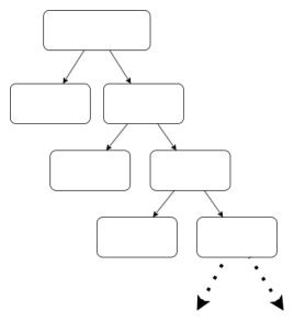
Figure 2.
Figures A and B illustrate how we check whether an agent collides with obstacle cells or another agent. Figure A depicts a circular agent, while Figure B shows a circular agent and a rectangular agent, with the cells they occupy filled with slashes. It is evident that in Figure A, the circular agent collides with the obstacle cells, and in Figure B, the circular and rectangular agents collide with each other.
Figure 2.
Figures A and B illustrate how we check whether an agent collides with obstacle cells or another agent. Figure A depicts a circular agent, while Figure B shows a circular agent and a rectangular agent, with the cells they occupy filled with slashes. It is evident that in Figure A, the circular agent collides with the obstacle cells, and in Figure B, the circular and rectangular agents collide with each other.
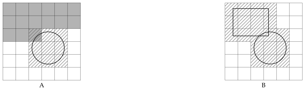
Figure 3.
Figure A shows a circular agent and a block agent, which occupy 9 and 2 cells respectively. Figure B illustrates the subgraph of the circular agent, and Figure C illustrates the subgraph of the block agent. In both subgraphs, each node represents an agent state, defined as a tuple consisting of a location and an orientation. Directed arrows represent the orientation of the nodes.
Figure 3.
Figure A shows a circular agent and a block agent, which occupy 9 and 2 cells respectively. Figure B illustrates the subgraph of the circular agent, and Figure C illustrates the subgraph of the block agent. In both subgraphs, each node represents an agent state, defined as a tuple consisting of a location and an orientation. Directed arrows represent the orientation of the nodes.
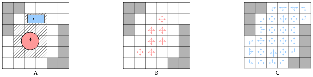
Figure 4.
Figure A shows a circular agent and a block agent exhibiting a vertex conflict. The conflict arises because their occupied cells overlap at the same timestep. Figure B illustrates a transfer (edge) conflict between two block agents. This conflict occurs when both agents transition from one state to another simultaneously, and their occupied cells overlap during the transition.
Figure 4.
Figure A shows a circular agent and a block agent exhibiting a vertex conflict. The conflict arises because their occupied cells overlap at the same timestep. Figure B illustrates a transfer (edge) conflict between two block agents. This conflict occurs when both agents transition from one state to another simultaneously, and their occupied cells overlap during the transition.
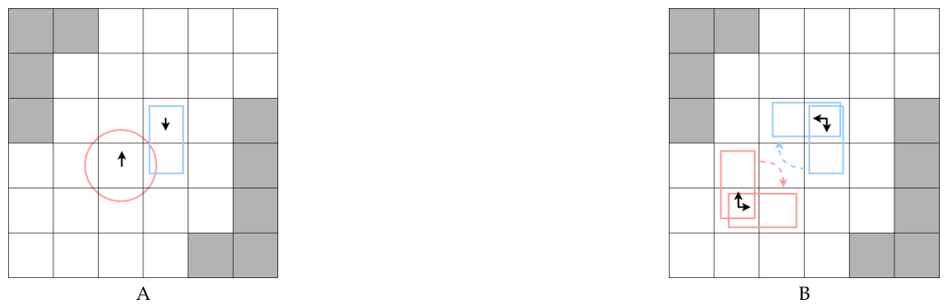
Figure 5.
Figure A shows a LA-MAPF problem with three agents: one block agent and two circle agents. We assume the agents can only move forward (i.e., move in their orientation) and change orientation by . Their start and target states are labeled as S1, T1; S2, T2; and S3, T3, respectively. All nodes in are shown in Figure B. The nodes in related to agent 2’s start or target (i.e., ) are shown in Figure C. Similarly, the nodes in related to agent 3’s start or target (i.e., ) are shown in Figure D.
Figure 5.
Figure A shows a LA-MAPF problem with three agents: one block agent and two circle agents. We assume the agents can only move forward (i.e., move in their orientation) and change orientation by . Their start and target states are labeled as S1, T1; S2, T2; and S3, T3, respectively. All nodes in are shown in Figure B. The nodes in related to agent 2’s start or target (i.e., ) are shown in Figure C. Similarly, the nodes in related to agent 3’s start or target (i.e., ) are shown in Figure D.
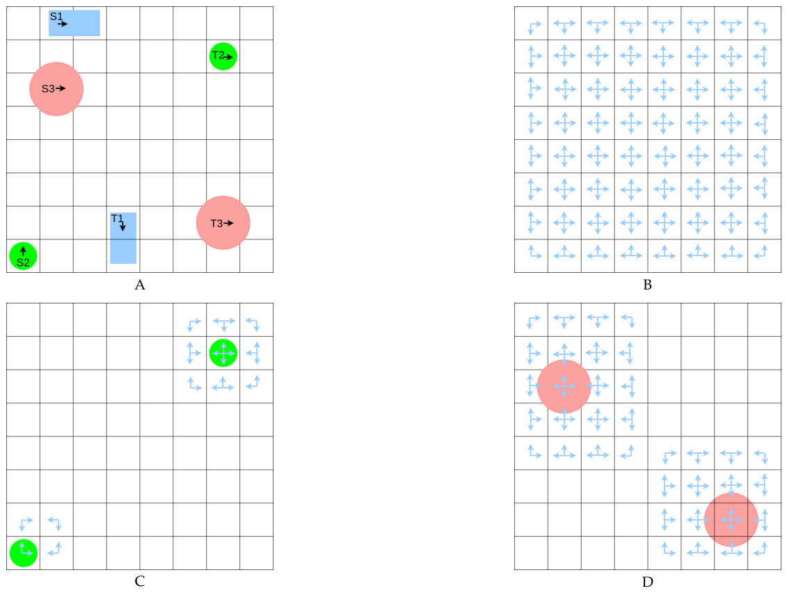
Figure 6.
This figure illustrates examples of what it means for an agent’s subgraph’s node to be related to another agent’s start or target. The blue rectangle represents agent 1 () in Figure 5 and the red circle represents the start state (S3) and target state (T3) of the third agent () in Figure 5. , , , and denote four states in agent 1’s subgraph . and are related to ’s start, because ; is also related to ’s start, because . But is not related to ’s start, because and for any state it can transfer to or from (denoted as ), and .
Figure 6.
This figure illustrates examples of what it means for an agent’s subgraph’s node to be related to another agent’s start or target. The blue rectangle represents agent 1 () in Figure 5 and the red circle represents the start state (S3) and target state (T3) of the third agent () in Figure 5. , , , and denote four states in agent 1’s subgraph . and are related to ’s start, because ; is also related to ’s start, because . But is not related to ’s start, because and for any state it can transfer to or from (denoted as ), and .
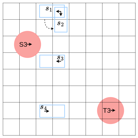
Figure 7.
These figures show a simple solvable MAPF problem (Figure A) and a simple unsolvable MAPF problem (Figure C). and represent the start and target cells of the three agents in the problem, as follows. For simplicity, all agents occupy just one cell. The paths of each agent in the problem are shown in Figures B and D, respectively. The problem in Figure A passes the solvability check, as all its agents have a path to their target. However, the problem in Figure C does not pass the solvability check and is unsolvable because only the 3rd agent has a path to its target, while the 1st and 2nd agents have no path to their target. Grey cells represent unpassable cells, while white cells represent passable cells, as follows.
Figure 7.
These figures show a simple solvable MAPF problem (Figure A) and a simple unsolvable MAPF problem (Figure C). and represent the start and target cells of the three agents in the problem, as follows. For simplicity, all agents occupy just one cell. The paths of each agent in the problem are shown in Figures B and D, respectively. The problem in Figure A passes the solvability check, as all its agents have a path to their target. However, the problem in Figure C does not pass the solvability check and is unsolvable because only the 3rd agent has a path to its target, while the 1st and 2nd agents have no path to their target. Grey cells represent unpassable cells, while white cells represent passable cells, as follows.
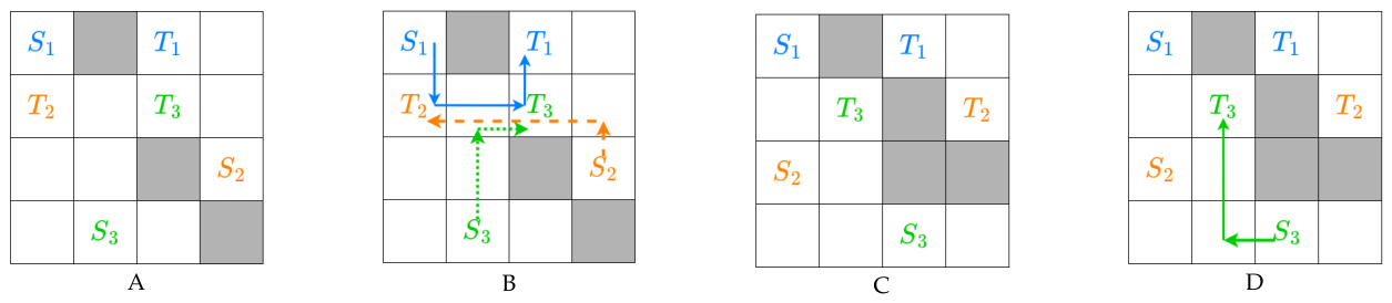
Figure 8.
This figure shows a simple LA-MAPF problem that passes the mentioned solvability check but is unsolvable. All agents occupy just one cell. Both and have a path from their start (, ) to their target (, ) when considered in isolation, provided the other agent’s start and target cells are treated as passable. However, the problem is unsolvable because inevitably blocks the only path for .
Figure 8.
This figure shows a simple LA-MAPF problem that passes the mentioned solvability check but is unsolvable. All agents occupy just one cell. Both and have a path from their start (, ) to their target (, ) when considered in isolation, provided the other agent’s start and target cells are treated as passable. However, the problem is unsolvable because inevitably blocks the only path for .
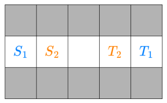
Figure 9.
These figures are based on the LA-MAPF problem shown in Figure 5. Figure A marks the range of nodes that may be related to other agents with dotted line rectangles. Figure B shows the nodes in that are related to other agents. Blue, green, red, purple, and yellow arrows represent nodes that have no relation to other agents, are related to , are related to , are related to , and are related to , respectively. And navy blue nodes represent the start and target states of . Figure C shows the generated from . The color of each node indicates its relationship with other agents, similar to Figure B. Figure E provides information about which nodes belong to which component. Some nodes of and their nearby nodes have the same relation with agents but are not in the same component, e.g., component 11, 7, 15. In this problem, because all agents can only move forward or rotate, some nodes are spatially adjacent but have no connecting edge between them, which prevents them from forming a directed cycle and thus excludes them from the same strongly connected component. Figure D is a simplified version of , containing only components that are related to other agents (i.e., components 1, 2, 3, 4) and components that contain ’s start or target nodes (i.e., components 1, 6). Each component’s related start state and target state are shown in brackets (e.g., S3” means start state of agent 3 and T1” means target state of agent 1). Ignored nodes have no influence on the relationship with other agents, so the simplified is equivalent to in determining an agent’s relationship with other agents. It is noteworthy that in Figure D, there is no direct connection between component 2 and component 6 , as there is no path in that connects components 2 and 6 without passing through 1 and 4.
Figure 9.
These figures are based on the LA-MAPF problem shown in Figure 5. Figure A marks the range of nodes that may be related to other agents with dotted line rectangles. Figure B shows the nodes in that are related to other agents. Blue, green, red, purple, and yellow arrows represent nodes that have no relation to other agents, are related to , are related to , are related to , and are related to , respectively. And navy blue nodes represent the start and target states of . Figure C shows the generated from . The color of each node indicates its relationship with other agents, similar to Figure B. Figure E provides information about which nodes belong to which component. Some nodes of and their nearby nodes have the same relation with agents but are not in the same component, e.g., component 11, 7, 15. In this problem, because all agents can only move forward or rotate, some nodes are spatially adjacent but have no connecting edge between them, which prevents them from forming a directed cycle and thus excludes them from the same strongly connected component. Figure D is a simplified version of , containing only components that are related to other agents (i.e., components 1, 2, 3, 4) and components that contain ’s start or target nodes (i.e., components 1, 6). Each component’s related start state and target state are shown in brackets (e.g., S3” means start state of agent 3 and T1” means target state of agent 1). Ignored nodes have no influence on the relationship with other agents, so the simplified is equivalent to in determining an agent’s relationship with other agents. It is noteworthy that in Figure D, there is no direct connection between component 2 and component 6 , as there is no path in that connects components 2 and 6 without passing through 1 and 4.
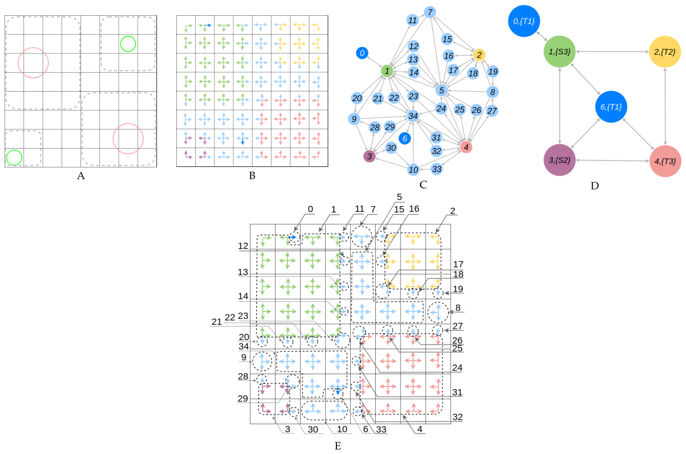
Figure 10.
This is a simplified component connectivity graph used to demonstrate how works. The graph corresponds to agent in a LA-MAPF problem involving three agents (, , ).
Figure 10.
This is a simplified component connectivity graph used to demonstrate how works. The graph corresponds to agent in a LA-MAPF problem involving three agents (, , ).
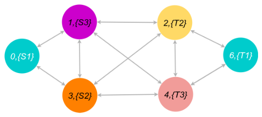
Figure 11.
This figure illustrates how to check whether the LA-MAPF problem in Figure 5 can be decomposed into three subproblems () under the simplified scenario. As shown in the figure, each subproblem has a solution (indicated by dotted lines) that avoids the target state of the previous subproblems and the start state of the next subproblems. Therefore, the problem can be decomposed into these three subproblems.
Figure 11.
This figure illustrates how to check whether the LA-MAPF problem in Figure 5 can be decomposed into three subproblems () under the simplified scenario. As shown in the figure, each subproblem has a solution (indicated by dotted lines) that avoids the target state of the previous subproblems and the start state of the next subproblems. Therefore, the problem can be decomposed into these three subproblems.
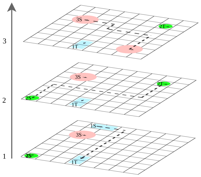
Figure 12.
This figure presents a simplified component connectivity graph of a MAPF problem involving four agents: , , , and . Here, and represent the start and target states of agent , respectively.
Figure 12.
This figure presents a simplified component connectivity graph of a MAPF problem involving four agents: , , , and . Here, and represent the start and target states of agent , respectively.
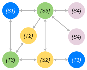
Figure 13.
The two figures show two different derived from two different dependency paths, along with the related subproblems.
Figure 13.
The two figures show two different derived from two different dependency paths, along with the related subproblems.
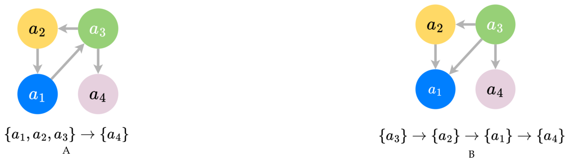
Figure 14.
Figure A illustrates three subproblems () and their solving order, indicated by solid arrows. The two dotted arrows represent potential new loops introduced by ’s dependency paths: the left dotted arrow corresponds to passing through the target states of , and the right dotted arrow corresponds to passing through the start states of . Figure B shows a solving order graph in which a loop involving four agents () exists. The left dotted arrow indicates an incoming edge from another agent in the same loop to , while the right dotted arrow indicates an outgoing edge from to another agent in the loop. If we can break one of these edges without introducing new loops, the original loop can be eliminated, resulting in a better decomposition.
Figure 14.
Figure A illustrates three subproblems () and their solving order, indicated by solid arrows. The two dotted arrows represent potential new loops introduced by ’s dependency paths: the left dotted arrow corresponds to passing through the target states of , and the right dotted arrow corresponds to passing through the start states of . Figure B shows a solving order graph in which a loop involving four agents () exists. The left dotted arrow indicates an incoming edge from another agent in the same loop to , while the right dotted arrow indicates an outgoing edge from to another agent in the loop. If we can break one of these edges without introducing new loops, the original loop can be eliminated, resulting in a better decomposition.
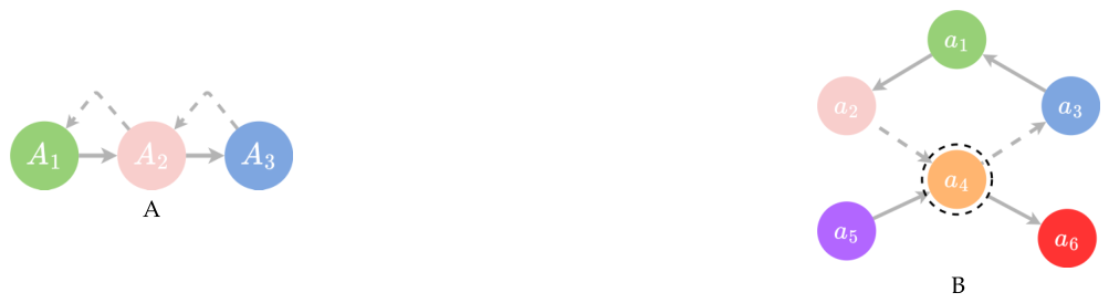
Figure 15.
In these figures, we present a solvable MAPF problem that our algorithm decomposes into unsolvable subproblems. Figure A demonstrates the start states and target states of three agents and the map. Our method may decompose this problem into two subproblems: . All subproblems pass the legality check; however, is unsolvable if we set subsequent subproblems’ start states to occupied, as can never reach its target state since blocks its way, as shown in Figure B. Then, according to our solvability safeguard, we ignore cells occupied by other subproblems’ start and target states and solve , the solutions are shown in Figures C and D. In Figure D, moves to (’s start state) to make way for to reach its target state; thus, is merged into . is solvable, and the solvability safeguard completes. Although this is an example of a MAPF problem, the same rules apply to LA-MAPF problems.
Figure 15.
In these figures, we present a solvable MAPF problem that our algorithm decomposes into unsolvable subproblems. Figure A demonstrates the start states and target states of three agents and the map. Our method may decompose this problem into two subproblems: . All subproblems pass the legality check; however, is unsolvable if we set subsequent subproblems’ start states to occupied, as can never reach its target state since blocks its way, as shown in Figure B. Then, according to our solvability safeguard, we ignore cells occupied by other subproblems’ start and target states and solve , the solutions are shown in Figures C and D. In Figure D, moves to (’s start state) to make way for to reach its target state; thus, is merged into . is solvable, and the solvability safeguard completes. Although this is an example of a MAPF problem, the same rules apply to LA-MAPF problems.
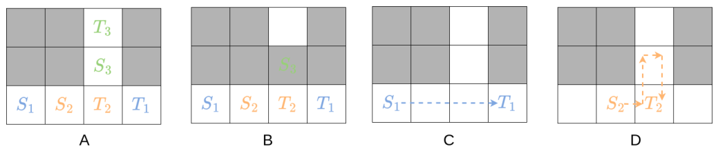
Figure 17.
This figure illustrates the map AR0203SR from the aforementioned dataset. It features 50 agents of various sizes, each with a path connecting its start and target states. As previously mentioned, 25 of the agents are circular, and the remaining 25 are rectangular.
Figure 17.
This figure illustrates the map AR0203SR from the aforementioned dataset. It features 50 agents of various sizes, each with a path connecting its start and target states. As previously mentioned, 25 of the agents are circular, and the remaining 25 are rectangular.
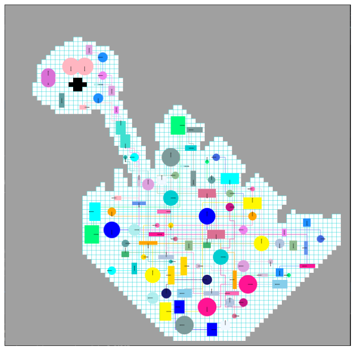
Figure 18.
These figures show partial time costs of the results in our experiments. In these results, BL increases the success rate of CBS substantially. More details can be found in Figure A1 and Figure A2.
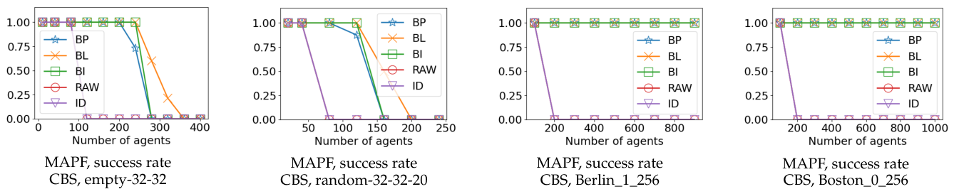
Figure 19.
These figures show partial success rate of the results in our experiments. In these results, BL increases the success rate of LaCAM substantially. More details can be found in Figure A4.
Figure 19.
These figures show partial success rate of the results in our experiments. In these results, BL increases the success rate of LaCAM substantially. More details can be found in Figure A4.
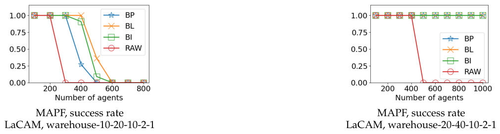
Figure 20.
These figures show partial success rate of the results in our experiments. In these results, BL increases the success rate of LA-CBS substantially. More details can be found in Figure A5 and Figure A6.
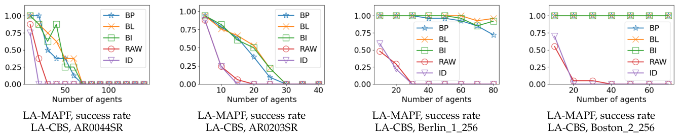
Figure 21.
These figures show partial success rate of the results in our experiments. In these results, BL increases the success rate of LA-LaCAM substantially. More details can be found in Figure A7 and Figure A8.
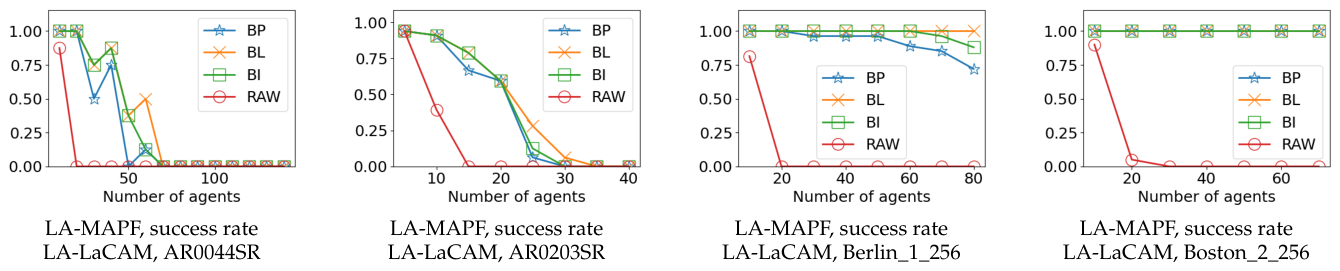
Figure 22.
These figures show partial time costs of the results in our experiments. There is no significant difference between the time cost of BI and BL on these maps. More details can be found in Figure A1, Figure A3, Figure A5, and Figure A7.
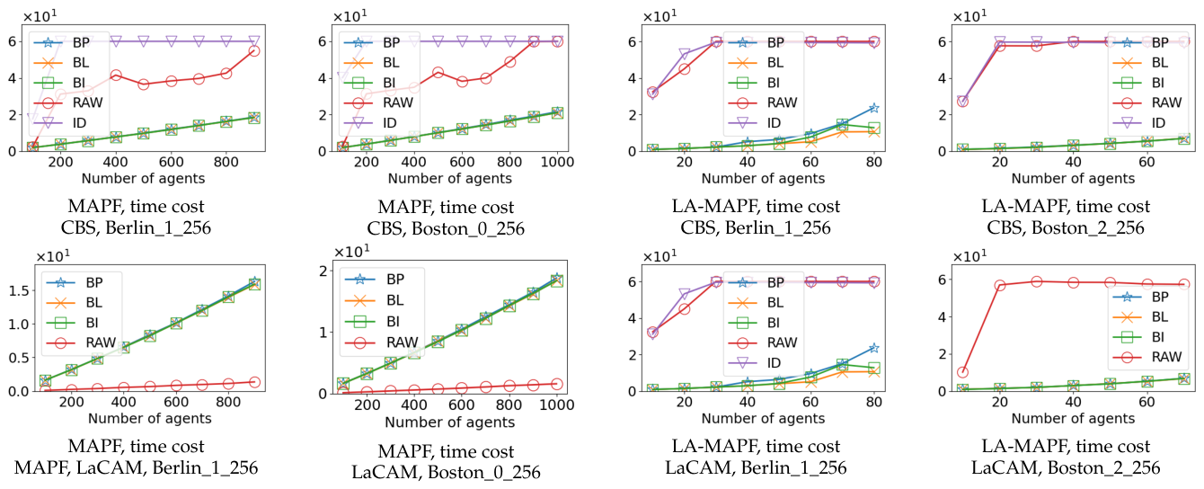
Figure 23.
These figures show partial time costs of the results in our experiments. There is significant difference between the time cost of BI and BL on these maps. More details can be found in Figure A1, Figure A4, Figure A6, and Figure A7.
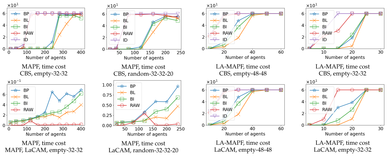

Table 1.
Comparison on CBS in average.
| Method | RAW | ID | BP | BL | BL_INIT |
| Time cost (s) | 35.54 | 55.16 | 9.81 | 7.21 | 8.21 |
| Success rate | 0.13 | 0.10 | 0.75 | 0.88 | 0.87 |
| Max subproblem size | - | 457.4 | 61.4 | 50.2 | 54.6 |
| Number of subproblem | - | 2.52 | 396.6 | 507.8 | 403.7 |
| Decomposition time cost (s) | - | - | 0.37 | 0.30 | 0.27 |
Table 2.
Comparison on CBS in average (makespan).
| RAW | ID | BP | BL | |
| RAW | - | 172.9 / 172.9 | 204.4 / 1484.8 | 204.4 / 1469.0 |
| ID | - | - | 172.9 / 890.6 | 172.9 / 897.9 |
| BP | - | - | - | 10647.4 / 10529.6 |
| BL | - | - | - | - |
Table 3.
Comparison on CBS in average (sum of cost).
| RAW | ID | BP | BL | |
| RAW | - | / | / | / |
| ID | - | - | / | / |
| BP | - | - | - | / |
| BL | - | - | - | - |
Table 4.
Comparison on LaCAM in average.
| Method | RAW | BP | BL | BL_INIT |
| Time cost (s) | 7.93 | 8.09 | 6.68 | 7.94 |
| Success rate | 0.90 | 0.93 | 0.96 | 0.90 |
| Max subproblem size | - | 55.1 | 45.6 | 52.6 |
| Number of subproblem | - | 400.5 | 412.4 | 386.1 |
| Decomposition time cost (s) | - | 0.37 | 0.30 | 0.27 |
Table 5.
Comparison on LaCAM in average (makespan).
| RAW | BP | BL | |
| RAW | - | 310.5 / 10784.9 | 309.9 / 10663.2 |
| BP | - | - | 10679.4 / 10587.9 |
| BL | - | - | - |
Table 6.
Comparison on LaCAM in average (sum of cost).
| RAW | BP | BL | |
| RAW | - | / | / |
| BP | - | - | / |
| BL | - | - | - |
Table 7.
Comparison on LA-CBS in average.
| Method | RAW | ID | BP | BL | BL_INIT |
| Time cost (s) | 54.25 | 55.13 | 21.91 | 19.79 | 22.79 |
| Success rate | 0.11 | 0.10 | 0.52 | 0.73 | 0.65 |
| Max subproblem size | - | 40.97 | 19.77 | 16.31 | 18.85 |
| Number of subproblem | - | 1.76 | 17.95 | 24.41 | 22.87 |
| Decomposition time cost (s) | - | - | 0.378 | 0.168 | 0.161 |
Table 8.
Comparison on LA-CBS in average (makespan).
| RAW | ID | BP | BL | |
| RAW | - | 231.23 / 228.08 | 234.07 / 261.0 | 234.07 / 263.15 |
| ID | - | - | 236.03 / 260.16 | 236.03 / 263.47 |
| BP | - | - | - | 488.59 / 484.99 |
| BL | - | - | - | - |
Table 9.
Comparison on LA-CBS in average (sum of cost).
| RAW | ID | BP | BL | |
| RAW | - | 1178.2 / 2268.3 | 1349.6 / 1483.4 | 1349.6 / 2476.7 |
| ID | - | - | 2348.0 / 1336.0 | 2348.0 / 1331.7 |
| BP | - | - | - | 8149.7 / 7700.5 |
| BL | - | - | - | - |
Table 10.
Comparison on LA-LaCAM in average.
| Method | RAW | BP | BL | BL_INIT |
| Time cost (s) | 52.32 | 23.62 | 17.14 | 19.78 |
| Success rate | 0.11 | 0.58 | 0.78 | 0.71 |
| Max subproblem size | - | 19.40 | 16.86 | 18.11 |
| Number of subproblem | - | 13.30 | 28.83 | 24.59 |
| Decomposition time cost (s) | - | 0.38 | 0.18 | 0.16 |
Table 11.
Comparison on LA-LaCAM in average (makespan).
| RAW | BP | BL | |
| RAW | - | 358.2 / 290.3 | 358.2 / 286.1 |
| BP | - | - | 593.5 / 605.3 |
| BL | - | - | - |
Table 12.
Comparison on LA-LaCAM in average (sum of cost).
| RAW | BP | BL | |
| RAW | - | 1638.3 / 1436.4 | 1638.3 / 1425.4 |
| BP | - | - | 9938.4 / 9266.4 |
| BL | - | - | - |
Disclaimer/Publisher’s Note: The statements, opinions and data contained in all publications are solely those of the individual author(s) and contributor(s) and not of MDPI and/or the editor(s). MDPI and/or the editor(s) disclaim responsibility for any injury to people or property resulting from any ideas, methods, instructions or products referred to in the content. |
© 2026 by the authors. Licensee MDPI, Basel, Switzerland. This article is an open access article distributed under the terms and conditions of the Creative Commons Attribution (CC BY) license (http://creativecommons.org/licenses/by/4.0/).
Copyright: This open access article is published under a Creative Commons CC BY 4.0 license, which permit the free download, distribution, and reuse, provided that the author and preprint are cited in any reuse.


