Submitted:
27 May 2026
Posted:
28 May 2026
You are already at the latest version
Abstract
Teledermatology has the potential to improve access to dermatological care in resource-limited settings, particularly for infectious skin diseases and Neglected Tropical Diseases (NTDs), where diagnostic capacity is often limited. This study aims to evaluate the feasibility of an artificial intelligence (AI) - based Teledermatology system, to support the classification of infectious versus non-infectious skin lesions. A convolutional neural network based on the ResNet50 architecture was trained on a dataset of dermatological images and optimized for deployment on a low-cost embedded device (Raspberry Pi 3). The system was designed to operate locally and includes a user interface for image acquisition, local storage, and cloud synchronization via Google Drive to enable remote consultation. The proposed model achieved an overall classification accuracy of 96% and a sensitivity of 89% for infectious lesions on the evaluated dataset, indicating its potential usefulness as a triage and decision-support tool for frontline healthcare workers. These findings suggest that AI-enabled Teledermatology systems deployed on affordable hardware may offer a scalable and cost-effective approach to supporting earlier identification of infectious cutaneous conditions, including NTDs, in underserved regions.
Keywords:
artificial intelligence
; teledermatology
; neglected tropical diseases
; convolutional neural network
; infectious skin diseases
; global health
1. Introduction
Neglected Tropical Diseases (NTDs) are a group of infectious diseases found in tropical and subtropical climates, primarily affecting populations living in extreme poverty. Although they affect more than 1.5 billion people worldwide, they have historically remained on the sidelines of global health initiatives, receiving disproportionately low attention, funding and investment in research compared to other diseases such as HIV/AIDS, malaria, or tuberculosis [1]. Their neglect is not due to their low prevalence, but rather because the populations they affect are socioeconomically invisible: communities that are politically unrepresented and have no way to robustly defend their rights [2].
NTDs proliferate precisely in places where access to clean water, sanitation, adequate housing and medical care is very limited. Therefore, they are closely related to the social determinants of health, and their persistence indicates deep-rooted patterns of inequality. Many NTDs cause chronic, disfiguring and disabling problems rather than high mortality, making them even more marginalized in policy decisions, typically based on mortality statistics. Yet, they have a significant impact on public health. NTDs cause more than 14.1 million disability-adjusted life years (DALYs) annually, and diseases such as leprosy, onchocerciasis, lymphatic filariasis and Buruli ulcer disease cause significant long-term suffering, stigmatization and exclusion [3].
Ultimately, NTDs have a multidimensional impact: affected individuals are often socially isolated, face barriers to education and employment, psychological trauma and economic dependence. This ultimately reinforces the cycle of poverty, affecting more to women and children, who bear additional burdens due to gender norms and caregiving roles [4]. Figure 1 is a visual representation of various neglected tropical diseases, their modes of transmission, and the types of pathogens (protozoan, helminthic, echinococcosis, fungal, bacterial, non-viral) involved in their spread, categorized by transmission methods such as vectors, direct contact, and environmental factors.
Recently, digital health tools have been increasingly becoming a big aid in the fight against NTDs. Mobile health (mHealth) applications, telemedicine platforms and AI-based diagnostic systems are very useful in overcoming geographical and infrastructure barriers, especially for cutaneous NTDs, which often produce visible lesions that allow for image analysis and remote consultation [2].
Neglected Tropical Diseases (NTDs) are endemic in many low- and middle-income countries (LMICs), where poverty, weak health systems, limited specialist availability, and poor infrastructure lead to delayed diagnosis and underreporting, particularly for cutaneous NTDs. Although mobile broadband coverage is widespread, digital health use remains limited, underscoring the need for affordable, offline-capable solutions. The Gulf of Guinea, specifically Benin, Côte d’Ivoire, Ghana, and Togo, represents a strategic focus due to high endemicity of multiple cutaneous NTDs and significant gaps in diagnostic capacity. These settings are well suited for deploying AI-supported, image-based diagnostic tools that align with long-term national strategies and global priorities such as the WHO 2021–2030 Roadmap for NTDs and Sustainable Development Goal 3.3. [6,7]
Figure 2.
Geographical and strategic context of challenges in NTD control in Low- and Middle-Income Countries (LMICs) and Gulf of Guinea.
Figure 2.
Geographical and strategic context of challenges in NTD control in Low- and Middle-Income Countries (LMICs) and Gulf of Guinea.

The integration of artificial intelligence (AI)-based systems into teledermatology workflows has the potential to improve the early detection and triage of infectious skin diseases in resource-limited settings. Recent advances in medical imaging and deep learning have demonstrated promising performance in the classification of dermatological conditions under controlled experimental settings. However, significant challenges remain regarding clinical generalizability, dataset diversity, infrastructure limitations, and deployment in low-resource environments. Addressing these challenges is essential for the development of scalable and clinically relevant AI-assisted teledermatology systems.
2. Materials and Methods
2.1. Telemedicine and Teledermatology
Teledermatology has been widely applied in the management and diagnosis of skin-related neglected tropical diseases (NTDs), using both real-time consultation and store-and-forward approaches [2]. There are several projects using real-time teledermatology consultations, such as those conducted in Taiwan using Intouch Lite software, that have also shown good patient satisfaction and clinical efficacy. For conditions like scabies that have very specific signs in the skin, doing immediate dermoscopic examinations remotely allows the doctors to diagnose very fast [8].
Table 1 summarizes key characteristics of existing digital health solutions addressing skin-related Neglected Tropical Diseases (NTDs), highlighting substantial heterogeneity in scope, technology, and performance.
Most tools are designed to support diagnosis, training, or case management of multiple cutaneous NTDs, while some focus on a single disease, such as leishmaniasis. Mobile applications are predominant technology, complemented by SMS-based teleconsultation systems and more complex teledermatology platforms, including robotic microscopy. Offline functionality is incorporated in several mobile apps to accommodate resource-limited settings, whereas real-time telemedicine solutions depend on stable internet connectivity. Most platforms integrate teleconsultation features to connect frontline health workers with specialists.
Diagnostic accuracy varies widely, with mobile applications reporting moderate to high performance and real-time systems achieving higher accuracy, largely influenced by image quality and algorithm design. Initial user engagement is generally high, although sustaining long-term use remains challenging, particularly for highly specialized tools. Common implementation challenges include infrastructure constraints, data security concerns, variable image quality, and inconsistent user adherence.
Cost-effectiveness also differs, with SMS-based systems being more affordable than hardware-intensive solutions. Overall, the solutions are primarily intended for rural and underserved settings. Future research should prioritize improving diagnostic accuracy, ensuring scalability and data security, expanding regional integration, and conducting comprehensive cost-effectiveness analysis to support sustainable implementation [8,9,10,11].
2.2. Solutions based on Raspberry Pi for Teledermatology
Alaidi et al. [12] show how they comprehensively implemented a monkeypox diagnostic system using AI and the Raspberry Pi 5. Their project incorporates a convolutional neural network (CNN) developed to identify skin symptoms such as smallpox from patient images. They decided to use the Raspberry Pi because they needed a portable detection system that did not necessarily require a connection, as outbreak-prone areas lack adequate resources.
Singh et al. [13] developed a prototype that uses a Raspberry Pi and classifies cutaneous signs using a CNN trained with melanoma images from the ISIC archive.
Srinivasan et al. [14] developed a public health-focused project consisting of two parts: an automated screening booth with a Raspberry Pi and an Artificial Neural Network (ANN). The goal is to combine AI with human-computer interaction to enable early detection of skin cancer in public spaces.
Based on this analysis (Table 2), Raspberry Pi emerges as a cost-effective and portable platform with sufficient computational capability to support optimized neural networks, thereby representing a promising solution for teledermatology applications in underserved settings. The availability of recent models, such as the Raspberry Pi 5, together with integrated AI accelerators, further enhances its suitability for deploying AI-driven systems of this nature.
2.3. Cloud-Based AI Platforms: Google Cloud for Skin Diseases
Although we have seen that non-cloud implementations can be very useful, the arrival of cloud computing has undoubtedly revolutionized the implementation and scalability of AI solutions in the healthcare field. One of the most widely used platforms in this area is Google Cloud Platform (GCP), which offers integrated tools for data storage, computing, and machine learning (ML).
In the context of teledermatology, GCP offers very useful features through its AutoML Vision and Google Vision APIs, which enable image classification and recognition for diagnostic support.
AutoML Vision has an intuitive interface for training custom machine learning models with minimal programming, which is perfect for facilitating access to AI tools for healthcare professionals without extensive technical knowledge. It is particularly useful in resource-limited settings, as it enables automated training, evaluation, and deployment of deep learning models using labeled images, such as those of skin signs, directly on the cloud infrastructure [15].
Several studies have shown that using this feature is feasible and diagnostically effective in various medical imaging areas such as skin lesions, retinal images, and chest X-rays. For example, Faes et al. [16] demonstrated that AutoML achieves specificity levels between 67% and 100% in multiclass classification tasks with dermatological images. Furthermore, data is secure within the Google Cloud ecosystem, as access is authenticated and encrypted, addressing key concerns about patient data privacy. The platform also facilitates real-time collaboration between healthcare teams and researchers globally, improving clinical decision-making. Furthermore, Google Cloud can be seamlessly integrated with mobile apps and devices, paving the way for developing scalable telemedicine solutions tailored to rural and underserved regions [15]. These capabilities make Google Cloud a very good option for a project like the one we are working on.
3. Results
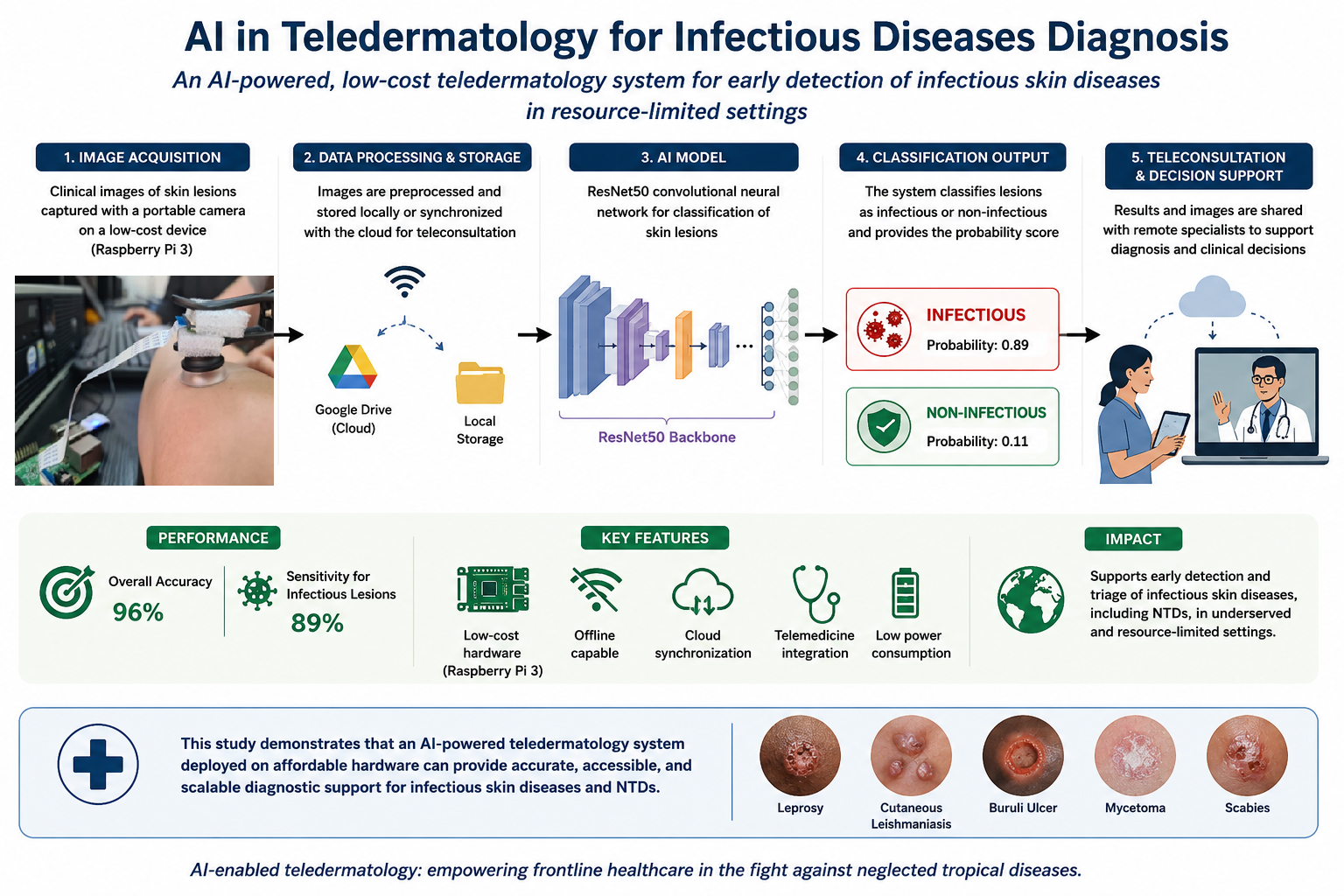
This paper presents the results of the developed platform, which was designed to address the key challenges identified in the current literature. The system integrates artificial intelligence for image analysis and lesion classification (infectious versus non-infectious) and is deployed on portable edge-computing hardware based on the Raspberry Pi 3, specifically targeting low-resource environments. The device is capable of fully offline operation, while also supporting cloud connectivity via Google Cloud when internet access is available. This hybrid architecture enables autonomous use in remote settings and facilitates expert consultation under connected conditions.
The platform was developed in collaboration with the Anesvad Foundation, a non-governmental organization with extensive experience in the management of cutaneous neglected tropical diseases (NTDs) in endemic regions. Their involvement ensured that the proposed solution is aligned with real-world clinical workflows and can be integrated into existing healthcare systems in resource-constrained settings.
The goal of this research is to develop an integrated teledermatology platform based on image classification with AI that addresses the challenges faced in diagnosing skin NTDs.
The specific infectious diseases and their clinical importance that we included in the study are explained in Table 3.
The non-infectious controls were Atopic Dermatitis, Eczema, Psoriasis, Contact Dermatitis, Benign Tumors, Malignant tumors (melanoma, BCC, SCC), Genetic skin diseases, Systemic disease manifestations. The excluded conditions were nail disorders.
3.1. System Architecture
Our system architecture consists of a hardware component responsible for image acquisition, a software component where we include our CNN, and a cloud component for uploading the acquired images to the cloud. The architecture is broadly divided into data acquisition, data transmission, processing, and inference/diagnosis.
Figure 3.
System architecture diagram.

The stored data are processed by a deep learning model composed of two main stages. In the first stage, a ResNet50 convolutional neural network is employed as the backbone for feature extraction. The adopted architecture follows the standard ResNet50 design, consisting of five sequential stages that include convolutional layers, batch normalization, ReLU activation functions, as well as identity and convolutional residual blocks.
In the second stage, the features extracted by the ResNet50 backbone are passed to a custom fully connected classification head. This head comprises a linear layer with 2048 input features and 256 output features, followed by a ReLU activation function and a dropout layer with a rate of 0.3 to mitigate overfitting. The final output layer produces logits that represent the raw classification scores. These logits are subsequently subjected to a thresholding mechanism (e.g., pinf > 0.5) to enable binary classification.
The trained and optimized model is stored in the cloud to support version control and facilitate efficient deployment across local devices.
Once a model is trained and validated, the next step is to download and deploy it on the local Raspberry Pi. Using this implemented model, we can perform real-time classification of the images we acquire with the Raspberry Pi itself. The result is a binary prediction: "INFECTIOUS" or "NON-INFECTIOUS," which serves as triage, and both the image and the classification can be sent to a medical professional. This would provide a clinical decision support tool that helps the physician make a final pathological diagnosis.
3.2. Data Collection and Preprocessing
For any AI model to be reliable and generalized adequately, the training data must be high-quality, diverse, and representative. In the current context of NTDs, the challenge is even greater because there is no available data representing these diseases, as the Anesvad Foundation stated when we requested images to develop the model. It is also very difficult to obtain images of patients with darker skin tones or from certain geographic regions. This section details the design, sources, selection criteria, and preprocessing techniques we used to build a robust dataset suitable for binary classification of skin lesions into infectious and non-infectious categories.
Data Sources
We obtained all the images used in this project from the publicly available Skin Diseases, DermNet dataset hosted on Kaggle [17]. This dataset contains thousands of curated dermatological images originally sourced from DermNet New Zealand, a reputable open-access resource managed by dermatologists.
The dataset consists of non-dermatoscopic clinical photographs, taken in natural light, depicting a wide range of dermatological diseases across various anatomical regions and skin types. From the entire repository, we extracted a subset of images corresponding to 23 disease categories, which we manually reclassified into a binary taxonomy: infectious and non-infectious (see Table 4). We performed the reclassification following the clinical dermatology literature.
In total, we included in the working dataset:
- ✓
- 1,204 images labeled as infectious
- ✓
- 3,615 images labeled as non-infectious
This class imbalance reflects the nature of the original dataset, in which infections are underrepresented (25% compared to 75% non-infectious), and this has influenced the modelling strategy.
These images were already divided into three folders in the dataset itself: train, test, and validation, and we decided to respect this division. Therefore, our project dataset is divided into six folders:
- ✓
- 959 images belonging to the infectious train set (80% of the infectious set)
- ✓
- 100 images belonging to the infectious test set (8% of infectious)
- ✓
- 145 images belonging to the infectious validation set (12% of infectious)
- ✓
- 2,880 images belonging to the non-infectious train set (80% of the non-infectious set)
- ✓
- 300 images belonging to the non-infectious test set (8% of non-infectious)
- ✓
- 435 images belonging to the non-infectious validation set (12% of non-infectious)
The training set was used for model optimization. The validation set was used to tune hyperparameters and early stopping. Finally, the validation and test sets were used for final model evaluation and metrics reporting.
To ensure clinical relevance and model integrity, included images were:
- ✓
- Images corresponding to confirmed dermatological diagnoses, based on original DermNet metadata.
- ✓
- Cropped images that lack watermarks, logos, or overlays that could bias the model.
Images in standard JPEG/PNG format with sufficient resolution. We verified that they were at least 300 pixels wide or high.
3.3. Preprocessing Pipeline
Several preprocessing steps were applied to the raw data using Python scripts to prepare the dataset for CNN training.
All images had a white text watermark in the center (see Figure 4), which could introduce spurious correlations during training because it can lead the model to associate background text features with class labels. Therefore, we attempted to remove it from the image using OpenCV's inpainting technique.
A quick look at the images showed that image restoration cleaned up some of the watermark elements, but it was image-specific and introduced quite a few artifacts (Figure 4). Additionally, the process sometimes removed non-text regions (e.g., bright highlights on skin or scar edges) if they exceeded a threshold.
For these reasons, we ultimately decided not to include this approach in the final preprocessing process. The next strategy was to avoid the watermark by cropping up the images (see Figure 5).
The original dataset was organized by disease category, with each folder containing images associated with a specific diagnosis. However, to make the binary classification task (distinguishing between infectious and non-infectious diseases) easier, we simplified and reorganized the data. We categorized each image to correspond to one of two labels based on the nature of the disease (e.g., fungal, bacterial, viral, or parasitic for infectious diseases; autoimmune, inflammatory, neoplastic, or allergic for non-infectious diseases).
We implemented robust error handling to identify and skip corrupted or unreadable files in both scripts, using exception handling provided by PIL's UnidentifiedImageError. This ensured that the pipeline was fault-tolerant and could run unattended on large datasets. The result was a clean and standardized directory structure with preprocessed images categorized into six folders corresponding to the binary classes (infectious and non-infectious) and the three data splits.
3.4. Model Development
The core of our AI system is the model development stage. The algorithm we developed is designed to automatically classify dermatological images into two clinical categories: infectious and non-infectious diseases. This system is based on deep learning models, specifically convolutional neural networks (CNNs), which have demonstrated very good performance in visual diagnostic tasks in dermatology.
As an exploratory step to improve the model's lesion localization capabilities, we decided to first program a classical computer vision workflow in Python to perform unsupervised segmentation of the images. We tested this method with examples of both infectious and non-infectious lesions to see if a basic thresholding and contour-based approach could isolate the region of interest (ROI), that is, the lesion area, from the background.
The segmentation had several parts. First, we loaded each image using OpenCV and converted it from BGR to RGB format for visualization. Then, we transformed it into grayscale to simplify pixel intensity analysis. We applied Otsu thresholding to the grayscale image using the cv2.THRESH_BINARY_INV + cv2.THRESH_OTSU flags. This adaptive method automatically determines an optimal global threshold value that separates the lesion (usually darker or textured) from the lighter skin or background. We inverted the binary mask we obtained in this step to make the dark regions the foreground. To identify external contours, we used cv2.findContours(). We assumed the largest contour by area was that of the main lesion. We drew a bounding rectangle around this contour to extract the ROI and created a copy of the original image with the contour overlaid for visualization.
Although the segmentation experiments provided qualitative insights into lesion localization, the approach was not integrated into the final classification pipeline due to inconsistent performance across heterogeneous dermatological images. Future work may explore more advanced segmentation methods, including attention-based deep learning architectures.
The visualization of each image has four panels (Figure 6): original image, binary segmentation mask, extracted ROI and original image with the lesion contour superimposed. With this technique, we got visually significant ROIs in many cases, especially when the contrast between the lesion and the surrounding skin was very strong. However, the results were more variable in other cases. Sometimes the algorithm misclassified skin folds or light reflections as foreground, thus segmenting the image incorrectly.
3.5. Architecture Selection
To begin the development process, we benchmarked two widely used CNN architectures: EfficientNet-B4 and ResNet50. We selected these two networks for their proven effectiveness in the literature for classifying dermatological images [18,19]. EfficientNet is a family of scalable and lightweight CNNs, introduced by Tan and Le in 2019 [20], which has become popular for its parameter efficiency and very high accuracy in computer vision tasks. ResNet50 is a red residual proposed by He et al. in 2015 [21], which is known for its simplicity and robustness, especially in clinical applications.
To compare these two architectures, we decided to implement two initial prototypes in separate Jupyter notebooks, using a reduced version of the dataset for faster experimentation: 400 images in total, which we split into train and test (80-20%). In ResNet, we initialized the model with pre-trained ImageNet weights and adapted it to binary classification by replacing its final fully connected layer with a custom head that outputs only a logit. We used the model's output in conjunction with the BCEWithLogitsLoss function, which combines two things: a sigmoid activation and a binary cross-entropy loss in a numerically stable way, resulting in efficient optimization for binary classification tasks. During this stage, we retrieved the selected images by connecting the notebook to Google Drive, where they are hosted in the /MyDrive/skinpatients folder. The data is organized into two subfolders: test infection/ and test non-infection/. The chosen images were resized to 224x224 pixels, and the training protocol used the Adam optimizer with a learning rate of 1x10⁻⁴, a batch size of 4 for 10 epochs, and the binary cross-entropy with logit loss objective function (BCEWithLogitsLoss). We evaluated performance using precision, recall, f1 score, support and a confusion matrix on a test set.
In EfficientNet, we used the same subset of images taken from Google Drive in the same way. We initialized it with pre-trained ImageNet weights and adapted it to binary classification by replacing its final layer with a custom head that outputs a single sigmoid value. The output was used in conjunction with the BCELoss loss function to enable optimization for binary classification tasks. The images were resized again, but this time to 380x380 pixels, and our CNN was trained using the Adam optimizer with a learning rate of 1×10⁻⁴ and a batch size of 4, for 10 epochs. We evaluated performance with the same metrics: precision, recall, F1-score, support and a confusion matrix on a test set.
In the results of this first test, we saw a trade-off between overall accuracy and sensitivity to the minority class. While ResNet50 achieved higher overall accuracy (74% vs. 57%) and better performance for the majority class (non-infectious lesions), EfficientNet-B4 demonstrated substantially higher sensitivity for the minority class (infectious lesions), achieving a recall of 0.70 compared to 0.10 for ResNet50. Despite this, we decided to select ResNet as the final architecture because it performed more consistently across different epochs and achieved much higher accuracy. However, this model needed some changes before training, validation and testing on all images.
3.6. Final Model
Previous CNNs were limited, it was just a test: we split the dataset into training and testing using train_test_split, which does not give us a reliable way to monitor the model's generalization during training. Furthermore, at that time, we had not yet included early stopping in the training process, which increased the risk of overfitting. As we already knew, there was also a significant class imbalance between infectious and non-infectious samples, which could bias the model toward the majority class, so it was very important to address this.
To address all these limitations, we introduced several methodological improvements in the improved version (Table 5). First, we decided to load the dataset from Google Drive directly into the three subsets we had prepared during data preprocessing: training, validation, and testing, so we could monitor performance in real time and retain the best model based on the validation loss. We added early stopping with a patience of 5 epochs, stopping training when we saw no improvement in the validation loss, thereby improving generalization. We addressed class imbalance by calculating a pos_weight parameter based on the ratio of negative and positive samples in the training set and integrating it into the BCEWithLogitsLoss function, which increased the model's sensitivity to the minority class, in this case, infectious diseases. Additionally, we increased the batch size from 4 to 16 and the maximum number of epochs from 10 to 20, which allowed for more stable gradient updates and improved convergence. We included resizing 224x224 pixels and normalization using ImageNet statistics to ensure the input data had a standardized range and distribution. Finally, instead of saving the final model, the refined pipeline tracks and saves the best-performing model (best_model_resnet.pth) based on the validation loss, thus ensuring optimal generalization performance in the version used for final evaluation.
To improve model robustness and reduce the risk of overfitting, data augmentation techniques were applied during training. These included horizontal flipping, random rotations, brightness adjustments, and scaling transformations. Augmentation was particularly important given the class imbalance and variability in dermatological image acquisition conditions.
At the end of the entire process, we decided to change the number of layers, comparing two architectures: ResNet50 (50 layers) and ResNet18 (18 layers), to choose the most suitable model for a limited computing environment, like the one we have with the Raspberry Pi. Both versions shared the same structure in terms of training logic, training hyperparameters, loss function and added classifier layers, the only difference being the base CNN architecture (ResNet18 vs. ResNet50), which differs in depth and number of parameters [22]. Our specific model has approximately 11.33 million parameters, which includes the pretrained ResNet-18 backbone and the custom classification head composed of two fully connected layers. Knowing each parameter is stored as a 32-bit floating point number (4 bytes), the total size of the model is around 43.2 megabytes.
To mitigate overfitting issues, we reduced the learning rate from 1×10⁻⁴ to 1×10⁻ in ResNet18, allowing for smoother and more stable convergence. We kept it at 1×10⁻⁴ in ResNet50.
In this case, although we found ResNet18 to be lighter and faster, we also know that it has a lower representation capacity. After the comparative analysis, we decided to continue with ResNet50 as the final system architecture, despite it having a bigger computational burden. We based our decision on its better performance in key metrics (accuracy, sensitivity, specificity), as well as its better ability to capture complex patterns in dermatological images. This robustness is very important given the tool's clinical objective as an AI-assisted triage system.
3.7. Integration with Raspberry Prototype
The device selected to build the prototype to be implemented was the Raspberry Pi 3 Model B, a low-power single-board computer developed by the Raspberry Pi Foundation. The hardware configuration includes a Pi board, a high-resolution camera module connected via the CSI interface, a USB Wi-Fi adapter for wireless connectivity, and a micro-USB power supply. The camera module allows for direct image acquisition, and the device has sufficient onboard capacity to perform local classification using the trained CNN model.
The Raspberry Pi 3 Model B features a 1.2 GHz quad-core 64-bit ARM Cortex-A53 CPU, 1 GB of RAM, and four USB 2.0 ports, in addition to an Ethernet port, HDMI output, a CSI camera interface, and a microSD card slot for boot and storage. It supports an HDMI display and GPIO interfaces for peripherals [23]. Despite not being the latest version, the Pi 3 Model B is still well-suited for low-power AI applications, especially where real-time GPU-based acceleration is not strictly required.
Figure 7.
Prototype including macro lens.

Performance evaluation on Raspberry Pi 3 Model B demonstrated an average inference time of approximately 420 ms per image, with average CPU utilization of 65% and memory usage of approximately 320 MB during inference. These results indicate that real-time offline deployment is feasible on low-cost embedded hardware platforms.
The goal of testing the macro lens was to see if it improved the visibility of fine-grained texture, edges, and surface features, which we thought might be important for diagnosis (e.g., whether there are scabs, ulcerations, or parasite burrows). However, capturing the image presented other challenges: there was less depth of field, it was more sensitive to motion blur, and the field of view was narrower, requiring more precise alignment and a stable mount during acquisition.
We also decided to create an acquisition protocol, whereby images are captured at a fixed distance of 10 cm from the skin using the standard settings, which would be without macro, and in direct contact with the skin using the macro settings. Standardizing these procedures ensures that all the images we capture follow the same framing, scale, and lighting conditions, which will ultimately improve the reliability of the model's predictions.
Figure 8.
Acquisition with macro lens.

3.8. User Interface and Software Inference
We developed the prototype's user interface using the Flask microframework, with the goal of creating a lightweight and accessible web application hosted locally on our Raspberry Pi. The interface can be accessed through any web browser over the local network and was designed to be simple, fast, and easy to use by healthcare professionals with no technical training.
Upon launching the system, the professional sees a structured form with two fields: the patient ID and the anatomical location of the lesion. Captured images are saved locally in the static/captures/ directory and can be immediately viewed within the web interface.
To allow remote collaboration, centralized data access and backups, we needed to integrate cloud storage into our teledermatology system, especially since we would likely need it for real-time diagnoses or for specialists to perform secondary reviews.
To achieve this, we incorporated a Google Drive-based cloud upload module into the system, implemented through the Google Drive API and protected by a dedicated service account.
Images are uploaded to the cloud using the MediaFileUpload protocol, which saves the structured file name, including the patient ID, injury site, and timestamp, so uploaded files remain traceable and well-organized. The system logs each upload for auditing purposes and allows re-uploading in the event of connectivity issues or failures.
To ensure security and privacy, we do not store or transmit sensitive personal data. The service account cannot access other Drive content and is limited to a single project folder. Future versions may integrate encryption at rest, user-level access control, and cloud-hosted inference, depending on the application context.
Using the Flask web framework again, app.py creates a local server that hosts an interactive graphical user interface (GUI), accessible from any device on the same local network.
While full regulatory certification falls beyond the scope of this academic research project, we have added several important assessments to make easier future clinical translation. Our preliminary evaluation against FDA Software as a Medical Device (SaMD) [24] Class II requirements identifies key gaps that would need addressing for regulatory submission at some point. Similarly, we analyze CE Marking requirements to understand the pathway for European deployment. Although the current prototype represents a research-stage system, future clinical translation would require formal software validation, cybersecurity assessment, usability testing, and compliance with Software as a Medical Device (SaMD) regulatory framework, including FDA and MDR requirements.
Ethical considerations are a very important part, with all prospective data collection done under Institutional Review Board approved protocols. We implement GDPR-compliant anonymization techniques to protect patient privacy while maintaining data utility. The platform's design incorporates privacy-by-design principles, including on-device processing options and encrypted data transmission for cloud-based analyses.
We exclude from the current work more resource-intensive aspects of regulatory compliance. Future steps are full 510(k) submission processes, post-market surveillance studies, and point-of-care device certification, as that would require additional partnerships and funding beyond this project's scope. However, our documentation approach ensures all necessary technical files and risk management documentation (per ISO 14971 [80]) are prepared to support such future endeavors.
In parallel, we have structured the system architecture and software lifecycle following the best practices described in the IEC 62304 standard [25], which governs software development for medical devices. We maintain the source code, version control and traceability of changes throughout the project to facilitate the preparation of a future design history file (DHF). While the prototype does not make clinical decisions autonomously, we have integrated a neural network that acts as a triage tool, providing clinical suggestions based on automatic image analysis. The final decision always rests with a physician, positioning the system as a decision-making aid rather than a substitute for clinical judgment. To this end, we have implemented robust logging and tagging mechanisms to facilitate both traceability and audit readiness, both very important aspects in a future regulatory review. We also ensure design modularity, for example by separating inference logic from the user interface, data transmission and storage, which would simplify future validation and cybersecurity assessments when required by regulatory bodies.
We designed this prototype and algorithm following key principles of privacy by design, ensuring that we do not collect, process or store personally identifiable information (PII) unless explicitly necessary. We trained the CNN using completely anonymized, publicly available images, thus avoiding the use of sensitive data in the early stages of development. The only metadata entered by the user during image acquisition is a patient identification code and the anatomical region of the lesion. This data is manually provided through the web interface and used to label the image for traceability purposes. The system never captures or records names, dates of birth, contact information or full facial images.
3.9. Results and Evaluation
Recall that after comparing EfficientNet with ResNet, the final model we chose was ResNet. We then decided to compare ResNet18 with Resnet50 due to the difference in layers between the two, which translates into a difference in learning capacity and depth. Therefore, ResNet50 should be able to capture more complex features in images, but with a higher computational cost. We will have to evaluate whether it is worth it or whether it is better to stick with a simpler model, in case it yields good results.
The ResNet50 model has a batch size of 16, a maximum number of epochs of 20, a learning rate of 1×10⁻⁴, resizing to 224x224 pixels, and normalization with standard ImageNet parameters. We also added an early stopping strategy with a patience of 5 epochs to avoid overfitting and optimize training time.
The validation loss starts at 1.0356 and ends at 0.9565, indicating that the model is learning effectively. The training loss follows a very similar decreasing pattern (from 1.0660 to 0.9989), meaning there is no overfitting.
Out of 20 epochs, the model improved 10-fold. We achieved the best performance in epoch 20, so early stopping was not necessary, and the model benefited from training for the full 20 epochs.
Initial experiments performed using simplified training configurations and reduced datasets resulted in limited sensitivity for the minority infectious class, particularly for ResNet18 (recall = 0.17). To address this limitation, the final ResNet50 pipeline incorporated several methodological improvements, including class-weighted loss functions, validation-based model selection, early stopping, normalization, and optimized training parameters. These modifications significantly improved infectious lesion detection, increasing recall to 0.89 on the independent test set. This highlights the importance of balanced optimization strategies and robust validation procedures when working with imbalanced dermatological datasets.
In ResNet50, during training, we see how the loss on both the training and validation sets progressively improves, from 0.96 in the first epoch to 0.10 in subsequent epochs, reaching an optimal point before stopping intervened early (Table 6). The validation loss steadily decreases from 0.72 to a minimum of 0.087 at epoch 13. After five consecutive epochs with no improvement in the validation loss, training was stopped early (epoch 18), indicating convergence. We automatically save the best model for later evaluation.
We calculated the time for training using the time.time() function, showing that the CNN was quite efficient for its complexity, requiring only 16 minutes to complete training using the access that Google Colab gives us to NVIDIA T4 GPUs. This is because the model architecture is highly optimized and makes efficient use of computational resources, allowing for rapid iteration and deployment in our context (with limited infrastructure) without sacrificing performance.
On the test set, consisting of 400 samples (300 non-infectious and 100 infectious), the model achieved the classification metrics we see in Table 9.

Table 7.
Classification metrics.
| Metric | Non-Infectious Class | Infectious Class |
| Accuracy | 96% | |
| Precision | 0.96 | 0.96 |
| Recall | 0.99 | 0.89 |
| F1-score | 0.98 | 0.92 |
The model demonstrated high accuracy in both classes, indicating few false positives. Recall is slightly lower for the infectious class, reflecting the inherent difficulty of correctly identifying the minority class, although a recall of 0.89 still means high sensitivity.
Using a class-weighting strategy during training, we improved the model's ability to detect infectious cases by compensating for imbalances in the dataset. This is very important in clinical settings, where false negatives (undetected infections) have serious consequences.
The confusion matrix of the binary classification model is a visual summary of how well the model performed on the test set, classifying lesions as infectious or non-infectious. It is divided into four parts, representing, from left to right and top to bottom:
- ✓
- True Negative (TN): an image from a non-infectious disease (negative) and classified as non-infectious (negative)
- ✓
- False Positive (FP): an image from a non-infectious disease (negative) and classified as infectious (positive) (also known as a Type I error or false alarm).
- ✓
- False Negative (FN): an image from an infectious disease (positive) and classified as non-infectious (negative) (also known as a Type II error).
- ✓
- True Positive (TP): an image from an infectious disease (positive) and classified as infectious (positive) [26].
- ✓
- We correctly classified 296 images as non-infectious (TN).
- ✓
- We incorrectly predicted 4 non-infectious images as infectious (FP).
- ✓
- We missed 11 infectious images, and they were predicted as non-infectious (FN).
- ✓
- We correctly classified 89 images as infectious (TP).
Figure 9.
Confusion matrix results.

The model performs very well, especially at detecting non-infectious cases, as we get very few false positives.
Although we have already calculated some of them directly in the code (Table 8), it is worth mentioning that these values are used to calculate:
- Accuracy
Overall correct predictions. Accuracy answers the question “Out of all the predictions we made, how many were true?” [27].
- Precision (Positive Predictive Value)
Precision gives us the proportion of true positives to the number of total positives that the model predicts. It answers the question “Out of all the positive predictions we made, how many were true?” [27].
- Recall (Sensitivity or True Positive Rate)
Recall focuses on how good the model is at finding all the positives. Recall is also called true positive rate and answers the question “Out of all the data points that should be predicted as true, how many did we correctly predict as true?” [27].
- • Specificity (True Negative Rate)
Specificity focuses on how good the model is at finding all the negatives. Specificity is also called true negative rate and answers the question: “Out of all the data points that should be predicted as false, how many did we correctly predict as false?”
- F1-Score
It is the harmonic mean of precision and recall, useful when there is class imbalance. As we have seen there is a trade-off between precision and recall, so F1 can be used to measure how effectively our models make that trade-off.
One important feature of the F1 score is that the result is zero if any of the components (precision or recall) fall to zero. Thereby it penalizes extreme negative values of either component [85].
- Negative Predictive Value (NPV)
NPV focuses on how much you can trust a negative prediction. It answers the question: “Out of all the data points that were predicted as false, how many were actually false?” It reflects the proportion of true negatives among all negative predictions that the model made.
- False Positive Rate (FPR)
FPR focuses on how often the model incorrectly labels negatives as positives. It answers the question: “Out of all the data points that should be predicted as false, how many did we incorrectly predict as true?” It represents the proportion of false positives among all actual negatives and is the complement of specificity.
- False Negative Rate (FNR)
FNR focuses on how often the model misses positive cases. It answers the question: “Out of all the data points that should be predicted as true, how many did we incorrectly predict as false?” It represents the proportion of false negatives among all actual positives and is the complement of recall.
- Balanced Accuracy
Balanced Accuracy focuses on giving a fair evaluation of model performance when we have imbalanced datasets. It answers the question: “How well does the model correctly identify both positive and negative classes?” It is calculated as the average of recall and specificity, making sure that both classes are equally weighted in the final performance metric.
3.10. PR Curve
The precision-recall (PR) curve graphically represents the trade-off between precision and recall at different decision thresholds [28].
The area under the precision-recall curve (PR AUC) is a summary of the model's ability to maintain high precision and recall across all thresholds. A PR AUC close to 1.0 means the model is successfully identifying most positive cases with few false positives. A lower PR AUC means the model is failing to identify the minority (positive) class.
The ROC (Ranking Operating Characteristic) curve is a graph that shows the recall versus the false positive rate across several thresholds. The area under the ROC curve (AUC ROC) represents the probability that the model will classify a randomly selected positive instance higher than a randomly selected negative instance.
Although the ROC curve is widely used, when there is class imbalance (as in our case) it can offer an overly optimistic view [29]. This is because the false positive rate considers the large number of negative samples, which can mask the poor performance of the model in the minority class. This is why we chose to report the PR-AUC metric. This curve gives us more information when there is imbalance, as it focuses specifically on the precision and recall of the minority class. This is very important to distinguish between infectious and non-infectious skin lesions, where the minority class is precisely the clinically relevant disease.
For this analysis we obtained two graphs. The first one is the PR trade-off as a function of decision threshold (Figure 11).
Figure 10.
PR trade-off as a function of decision threshold.

This graph shows how precision and recalls change when adjusting the threshold used to determine whether a lesion is infectious. At lower thresholds (for example, <0.3), the model detects almost all infectious lesions (high recall) but also misclassifies some as non-infectious (lower precision). As we increase the threshold, precision improves (meaning predictions are more reliable), but recall decreases, so some infectious lesions may be missed.
If the priority is not to miss any infectious cases, it is beneficial to have the threshold slightly below the middle (for example, 0.4) to increase recall.
In Figure 11, we see the PR curve obtained for the final model, which shows a high level of performance, with an average precision (AP) or area under the curve (AUC) of 0.97. This means that the model distinguishes very well between infectious and non-infectious skin lesions. In this curve, we see that the model maintains high precision even with high recall levels, which is very important in medical applications where false negatives can have serious consequences. We need to reliably detect lesions of infectious origin, even in images that are not of the best quality. The model demonstrates high recall without sacrificing much precision, meaning it can detect most infectious cases and avoid many false positives, which are needed for the early detection and triage of NTDs.
Figure 11.
PR curve.

3.11. Predictions on Unseen Images
To evaluate the model's classification ability with data it has not previously seen, such as a patient image when using it in the field, we tested it with an image from another dataset that was not included in the training, validation, or test sets. The first is an image of a skin lesion that we know to be infectious. We first load the image using the PIL library and display it. We then preprocess it by resizing it to the input size required by the model, converting it into a normalized tensor. The model, pretrained and saved as best_model_resnet.pth, is loaded and set to evaluation mode.
We perform a forward pass without calculating gradients (torch.no_grad()) and pass the output through a sigmoid function to obtain a probability between 0 and 1. This probability is compared to a threshold (default value 0.5; but as we saw in Figure 21, we could lower it a bit) to determine the final class. We visualize the result, the predicted class (infectious or non-infectious) and the associated confidence level (Figure 23).
Figure 12.
Image predicted as infectious.

We repeat the process, this time uploading to the model an image that it has never seen and we know is non-infectious.
Figure 13.
Image predicted as non-infectious.

As we can see, the classification is done properly, so the model would be ready to be used as a form of triage in places with high prevalence of NTDs.
3.12. Raspberry Pi Results
We built the image capture step by step, improving an initial script. These first images were taken with the Thesis.py script (Figure 26). The next step was taking images with the app.py and app1.py scripts, both with and without macro lens for comparison.
Figure 14.
First images taken by the prototype.

Figure 15.
Image taken using the macro lens accessory, named1_arm_20250514_14224. The name is standardized and represents (the patient ID)_(lesion area)_(date)_(time with minutes and seconds). The name of every image follows this structure for traceability purposes.
Figure 15.
Image taken using the macro lens accessory, named1_arm_20250514_14224. The name is standardized and represents (the patient ID)_(lesion area)_(date)_(time with minutes and seconds). The name of every image follows this structure for traceability purposes.

Several limitations of the present study should be acknowledged. The dataset was derived primarily from publicly available DermNet images and may not fully represent the variability encountered in real-world clinical environments, particularly regarding skin tone diversity, acquisition conditions, and geographic variability. Furthermore, external validation on independent datasets was not performed and will be necessary before clinical implementation.
4. Discussion
4.1. Interpretation of Results
During the evaluation phase, we obtained results that confirm that the proposed teledermatology platform is perfectly viable, both from a technical and clinical perspective. The model architecture we ultimately chose, ResNet50, demonstrated very good generalization capabilities and achieved a validation loss of only 0.087, while also avoiding overfitting thanks to our use of early stopping. This demonstrates that the model has learned the underlying patterns in the images, especially once we made improvements to the preprocessing and training strategy.
Regarding the final classification performance, we achieved an accuracy of 96% and F1 scores of 0.98 and 0.92 for the non-infectious and infectious classes, respectively, even though the classes were not balanced. We achieved a recall value of 0.89 for the infectious class, which is very important in our context since we do not want to miss any infectious diseases. In the precision-recall analysis, we achieved a PR AUC of 0.97, which is highly significant since PR curves measure performance more realistically when performing unbalanced classification compared to ROC curves. Our model maintains a high level of precision even with high recall, making it ideal for triage in endemic areas.
Another important result is how the model processes previously unseen images. With this test, we were able to confirm the model's consistency when making decisions, suggesting that it is ready to be implemented in real-world environments with data we acquire in the field.
4.2. Challenges and Solutions
During the development of this project, we addressed several technical and contextual challenges. In this section, we explain these challenges and the strategies we followed to address them and make our teledermatology platform applicable in real-world settings.
4.2.1. Data Limitations
A major problem was that annotated datasets representing skin NTDs were very scarce or nonexistent. Many of the publicly available datasets are biased toward diseases common in high-income countries, such as melanoma or psoriasis.
Instead of focusing on each NTD, since neither the Anesvad Foundation nor the WHO itself has a sufficiently large database for each disease, we obtained sets that included infectious skin diseases, which would be a broader set that also encompasses NTDs.
Therefore, to maximize the value of the available data, we decided to focus on classifying between infectious and non-infectious diseases. We used transfer learning using a pre-trained ResNet50 as a feature extractor to avoid the need for large datasets, and we used class weighting during training to account for the imbalance between infectious and non-infectious samples.
4.2.2. Class Imbalance
In the dataset, there were still many more images of non-infectious diseases than infectious ones, with the latter being underrepresented, resulting in poorer performance.
To address this, we included a class-weighted loss function to further penalize errors in the minority class. Additionally, we used evaluation metrics such as the F1 score and the precision-recall AUC ratio to ensure the model could reliably detect infectious lesions.
4.2.3. Hardware Limitations
The device we decided to use for the implementation (Raspberry Pi) has limited computing power and memory, which limits the complexity of our model and the speed of inference.
To address this, we reduced the model size by replacing the default fully connected header with a lighter custom header. We implemented the optimized PyTorch model, which we converted to TorchScript for better compatibility. It is also worth mentioning that we only included essential libraries and modules in the implementation environment, thus reducing the system load.
4.2.4. Image Variability
The test images we took under different lighting conditions, at different distances, and at different angles introduced noise and inconsistencies into the input data.
To address this, we standardized the imaging process, creating a very specific protocol and housing for the device where the camera and other elements remained fixed. Regarding preprocessing, we also applied sizing and normalization adjustments before feeding the images into the CNN.
4.2.5. Feasibility of Implementation
We had to ensure that the device could work without an internet connection, or with an unreliable internet connection, and that the solution did not need to be implemented on high-end devices.
As a solution, we successfully implemented the AI model on a Raspberry Pi 3, with acceptable inference times and offline functionality. We included optional integration with Google Cloud when internet is available, to enable data synchronization and remote consultations.
4.3. Impact on Healthcare
By developing this teledermatology platform to aid in the diagnosis of infectious diseases and NTDs, we aimed to improve global health, especially in regions with less resources. Once fully implemented, we expect this system to:
- Strengthen primary care: in many low- and middle-income countries, especially in remote areas, FHWs are often the only point of care for people with skin conditions. However, they lack specialized dermatological training or decision-support tools. This platform supports FHW clinical triage, differentiating between infectious and non-infectious lesions and enabling non-specialized personnel to make better-informed decisions. Because it works offline, it is also an accessible and context-specific diagnostic tool.
- Early detection and improved case management: cutaneous NTDs often present visible signs; however, they are usually misdiagnosed or diagnosed too late. Diagnosing infectious diseases early leads to better treatment and minimizes long-term complications. It allows us to more quickly refer to serious or unclear cases, improving the prognosis and limiting transmission if it is a communicable disease. Better triage also optimizes medical resources, avoiding unnecessary treatments.
- Integration with public health surveillance: infectious skin diseases, especially NTDs, are often underreported, making them difficult to monitor. Since the platform can store images and classification data, digital records could be created to help with epidemiological monitoring. Ideally, these records would then be integrated with national health systems to monitor diseases and, for example, identify outbreak patterns.
- Promoting health equity: existing AI applications in dermatology primarily focus on diseases in developed countries. This project refocuses the approach toward underserved populations, addressing a significant gap that existed. The use of low-cost hardware ensures that the project will be scalable and affordable.
The project directly supports these global commitments. We have developed a practical, field-oriented design to also foster collaboration between researchers and NGOs, such as the Anesvad Foundation with which we work, and ministries of health to pursue broad implementation in the future.
5. Conclusions
This paper presented the design, implementation, and technical evaluation of a low-cost, AI-enabled teledermatology platform aimed at improving the diagnosis and triage of infectious skin diseases in sub-Saharan Africa. The proposed solution addresses both technological and healthcare challenges by combining deep learning, edge computing, and telemedicine workflows, with a strong focus on accessibility, robustness, and real-world applicability.
From a technical perspective, a deep learning–based binary classifier built upon the ResNet50 architecture was developed to distinguish between infectious and non-infectious skin lesions. Trained in real clinical images, the model achieved high performance across multiple evaluation metrics, including an overall accuracy of 96% and F1 scores of 0.98 and 0.92 for the respective classes. The use of class-weighted loss functions contributed to robustness against class imbalance, while evaluation on unseen data demonstrated reliable generalization, supporting the feasibility of deployment outside controlled environments.
A key contribution to this work is the successful integration of the model into low-cost edge computing hardware. Deployment on a Raspberry Pi 3 enabled real-time inference with minimal computational and energy requirements. The platform operates through a fully local workflow for image acquisition, preprocessing, prediction, and storage, thereby reducing dependence on continuous internet connectivity and cloud infrastructure, an essential consideration in resource-constrained settings.
In terms of clinical relevance, the binary classification strategy mirrors real-world triage logic by differentiating communicable from non-communicable conditions. This approach directly supports frontline healthcare workers in referral and decision-making processes, helps reduce unnecessary treatments, and facilitates earlier detection of potentially contagious diseases. As such, it aligns closely with public health priorities related to the management of neglected tropical diseases (NTDs).
The platform was also designed with practical teledermatology workflows in mind. Cloud synchronization capabilities enable teleconsultation and data sharing when connectivity is available, while system requirements were tailored to the contextual constraints of target regions, including Benin, Ghana, Côte d’Ivoire, and Togo. This design philosophy emphasizes deployability and usability rather than purely theoretical performance.
More broadly, this work contributes to global health and health equity efforts. It is aligned with the WHO Roadmap for NTDs (2021–2030) and Sustainable Development Goal 3.3, promoting innovation in neglected disease diagnostics, democratization of AI-based medical technologies, and progress toward fairer AI systems by addressing geographic, demographic, and socioeconomic biases prevalent in existing models.
Despite these contributions, several directions for future research and development remain. First, comprehensive clinical validation is required to assess the platform’s safety, usability, and effectiveness in real-world healthcare settings. This includes pilot deployments in endemic regions, close collaboration with local health systems and non-governmental organizations, and systematic collection of qualitative and quantitative feedback from healthcare professionals.
Model explainability also remains an important requirement for clinical adoption. Future iterations of the platform should integrate explainable AI techniques, such as Grad-CAM, to provide visual explanations, confidence scores, and decision indicators within the user interface. These features would support clinician trust and responsible use of the system.
Finally, regulatory, ethical, and sustainability considerations must be addressed prior to large-scale deployment. Compliance with applicable medical device regulations, data protection standards, and informed consent requirements are essential. In parallel, sustainable implementation strategies including healthcare worker training, device maintenance plans, and long-term local partnerships will be necessary to ensure lasting impact.
In conclusion, this paper demonstrates the technical feasibility and potential public health value of low-cost, AI-driven teledermatology systems for infectious disease triage in resource-limited settings. With further validation, expansion, and governance, such platforms could play a meaningful role in strengthening primary care, supporting healthcare workers, and reducing inequities in access to dermatological expertise.
Author Contributions
All authors contributed equally to the conception, methodology, analysis, writing, and revision of the manuscript. All authors have read and agreed to the published version of the manuscript.
Funding
This research received no external funding.
Institutional Review Board Statement
Not applicable.
Informed Consent Statement
Not applicable.
Data Availability Statement
Publicly available datasets were analyzed in this study. The dermatological image dataset used for model development was obtained from the DermNet dataset available through Kaggle. Processed data supporting the findings of this study are available from the corresponding author upon reasonable request.
Acknowledgments
The authors would like to acknowledge the support provided by Anesvad Foundation https://www.anesvad.org/en/, during the development of this work. During the preparation of this manuscript, the authors used ChatGPT (OpenAI, GPT-5) for language refinement and editorial assistance. The authors reviewed and approved all generated content and took full responsibility for the final manuscript.
Conflicts of Interest
The authors declare no conflicts of interest.
Abbreviations
The following abbreviations are used in this manuscript:
| NTDs | Neglected Tropical Diseases |
| AI | Artificial Intelligence |
| DALYs | disability-adjusted life years |
| WHO | World Health Organization |
| LMICs | low- and middle-income countries |
| ANN | Artificial Neural Network |
| CNNs | convolutional neural networks |
References
- World Health Organization, Ending the Neglect to Attain the Sustainable Development Goals: A Road Map for Neglected Tropical Diseases 2021–2030, Geneva, Switzerland: World Health Organization, 2021. Available: https://www.who.int/publications/i/item/9789240010352.
- E. J. Barnowska, A. Fastenau, S. Penna, A.-K. Bonkass, S. Stuetzle, and R. Janssen, Diagnosing skin neglected tropical diseases with the aid of digital health tools: A scoping review, PLOS Digital Health, vol. 3, no. 10, Oct. 2024. [CrossRef]
- World Health Organization, Neglected tropical diseases, World Health Organization, 2026, https://www.who.int/health-topics/neglected-tropical-diseases#tab=tab_2. (Accesed on 02.03.2026).
- N. A. Pastrana, D. Beran, C. Somerville, O. Heller, J. C. Correia, and L. S. Suggs, The process of building the priority of neglected tropical diseases: A global policy analysis, PLOS Neglected Tropical Diseases, vol. 14, no. 8, Aug. 2020, Art. no. e0008498. [PMCID: PMC7423089] . [CrossRef]
- A. Frej, Protocol and pilot test to assess the quality of performance of the Skin NTDs app: a diagnosing tool developed by the World Health Organisation for Neglected tropical diseases that primarily affect the skin: a cross-sectional study, 2021. https://dugi-doc.udg.edu/handle/10256/19902.
- World Health Organization, Global Report on Neglected Tropical Diseases 2023, Geneva, Switzerland: World Health Organization, 2023. https://www.who.int/publications/i/item/9789240067295.
- K. Bahia and A. Delaporte, The State of Mobile Internet Connectivity 2020, Connected Society, GSMA, London, UK, Sep. 2020. https://www.gsma.com/r/wp-content/uploads/2020/09/GSMA-State-of-Mobile-Internet-Connectivity-Report-2020.pdf.
- C.-H. Lee, C.-C. Huang, J.-T. Huang, C.-C. Wang, S. Fan, P.-S. Wang, and K.-C. Lan, Live-interactive teledermatology program in Taiwan: One-year experience serving a district hospital in rural Taitung County, Journal of the Formosan Medical Association, vol. 120, no. 1, Part 2, pp. 422-428, Jan. 2021. doi: . [CrossRef]
- M. Cano, J. A. Ruiz-Postigo, P. Macharia, Y. A. Amoako, R. O. Phillips, E. Kinyeru, and C. Carrion, Evaluating the World Health Organization’s SkinNTDs App as a Training Tool for Skin Neglected Tropical Diseases in Ghana and Kenya: Cross-Sectional Study, J. Med. Internet Res., vol. 26, 2024, doi: 10.2196/51628; https://www.jmir.org/2024/1/e51628.
- N. Mwageni et al., The NLR SkinApp: Testing a Supporting mHealth Tool for Frontline Health Workers Performing Skin Screening in Ethiopia and Tanzania, Trop. Med. Infect. Dis., vol. 9, no. 1, p. 18, Jan. 2024. [CrossRef]
- R. Yotsu et al., An mHealth App (eSkinHealth) for Detecting and Managing Skin Diseases in Resource-Limited Settings: Mixed Methods Pilot Study, JMIR Dermatol., vol. 6, p. e46295, 2023. [CrossRef]
- A. H. M. Alaidi, Z. A. Ramadhan, J. S. Alrubaye, H. T. S. ALRikabi, H. A. Mutar, and I. Svyd, AI-based monkeypox detection model using Raspberry Pi 5 AI Kit, Sustainable Engineering and Innovation, vol. 7, no. 1, 2025. doi: . [CrossRef]
- O. Jeba Singh, D. Lavanya, S. Mahapatra, R. Rajesh Sharma, A. Sungheetha, and R. Niranjana, Raspberry Pi Integrated CNN Method to Find the Skin Lesions from Photo Images, 2024 3rd Edition of IEEE Delhi Section Flagship Conference (DELCON), New Delhi, India, 2024, pp. 1-5, doi: 10.1109/DELCON64804.2024.10867073 ; https://ieeexplore.ieee.org/document/10867073.
- S. Srinivasan, G. Indra, T. R. Saravanan, S. Murugan, C. Srinivasan, and M. Muthulekshmi, Revolutionizing Skin Cancer Detection with Raspberry Pi-Embedded ANN Technology in an Automated Screening Booth, in 2024 4th International Conference on Innovative Practices in Technology and Management (ICIPTM), Noida, India, 2024, pp. 1-6, doi: 10.1109/ICIPTM59628.2024.10563383; https://ieeexplore.ieee.org/document/10563383.
- P. Subashini, T. Dhivyaprabha, M. Krishnaveni, and J. S. M. B., Smart Intelligent System for Cervix Cancer Image Clas-sification Using Google Cloud Platform, in Enabling Technologies for Effective Planning and Management in Sustainable Smart Cities, 2023, pp. 245–281, doi: 10.1007/978-3-031-22922-0_10. https://link.springer.com/chapter/10.1007/978-3-031-22922-0_10.
- L. Faes et al., Automated deep learning design for medical image classification by health-care professionals with no coding experience: a feasibility study, Lancet Digit Health, vol. 1, no. 5, pp. e232–e242, Sep. 2019, doi: 10.1016/S2589-7500(19)30108-6. https://pubmed.ncbi.nlm.nih.gov/33323271/.
- C. Tirumala, Skin Diseases DermNet, Kaggle, 2023. https://www.kaggle.com/datasets/chetantirumala/skin-diseases-dermnet/data.
- N. D. Reddy, Classification of Dermoscopy Images using Deep Learning, arXiv preprint arXiv:1808.01607, Aug. 2018. doi: 10.48550/arXiv.1808.01607. https://arxiv.org/abs/1808.01607.
- M. Defresne, E. Coutier, P. Fricker, F. A. A. Blok, and H. Nguyen, Interpretable AI for Dermoscopy Images of Pigmented Skin Lesions, Journée santé et IA - PFIA 2024, La Rochelle, France, Jul. 2024. https://hal.science/hal-04703835v1/file/ias2024_paper_2.pdf.
- M. Tan and Q. V. Le, EfficientNet: Rethinking Model Scaling for Convolutional Neural Networks, arXiv preprint arXiv:1905.11946, 2019. doi: 10.48550/arXiv.1905.11946. https://arxiv.org/abs/1905.11946.
- K. He, X. Zhang, S. Ren, and J. Sun, Deep Residual Learning for Image Recognition, arXiv preprint arXiv:1512.03385, 2015. doi: 10.48550/arXiv.1512.03385. https://arxiv.org/abs/1512.03385.
- Maharajpet, S. S., Manjunath, H., & Dixit, S. (2025). AI-Driven Hostel Monitoring System: Integrating Automated Attendance, Real-Time Visitor Detection, and Facial Recognition-Based Geo-Fencing Using. European Journal of Applied Science, Engineering and Technology, 3(3), 14-26. [CrossRef]
- 2024. Available online: https://www.raspberrypi.com/products/raspberry-pi-3-model-b/.
- U.S. Food and Drug Administration, Global Approach to Software as a Medical Device, FDA, 2 Aug. 2022. https://www.fda.gov/medical-devices/software-medical-device-samd/global-approach-software-medical-device.
- International Electrotechnical Commission, IEC 62304:2006 – Medical device software – Software life cycle processes, IEC, Geneva, Switzerland, May 2006. Available: https://www.une.org/encuentra-tu-norma/busca-tu-norma/iec?c=6792.
- Harikrishnan N B, Confusion Matrix, Accuracy, Precision, Recall, F1-Score, Medium, Jul. 5, 2019. https://medium.com/analytics-vidhya/confusion-matrix-accuracy-precision-recall-f1-score-ade299cf63cd.
- LabelF, What is Accuracy, Precision, Recall, and F1-Score?, LabelF Blog, https://www.labelf.ai/blog/what-is-accuracy-precision-recall-and-f1-score.
- J. Ramírez, PR and ROC Curves, Medium, Sep. 19, 2019. https://medium.com/bluekiri/pr-and-roc-curves-1489fbd9a527.
- Davis and M. Goadrich, The relationship between Precision-Recall and ROC curves, in Proc. 23rd Int. Conf. Mach. Learn. (ICML '06), Pittsburgh, PA, USA, 2006, pp. 233-240. [CrossRef]
Figure 1.
Neglected tropical diseases: Overview of the WHO NTD list, their main reservoir and mode of transmission [5]. Notes: * “Direct contact” includes skin-to-skin, environmental exposure, and maternal-fetal transmission depending on disease. ** Environmental reservoirs are suspected of diseases like Buruli ulcer and mycetoma.

Figure 4.
OpenCV preprocessing.

Figure 5.
Images before and after cropping.

Figure 6.
Unsupervised segmentation of the images.

Table 1.
NTDs Digital Tools comparison.
| Feature | SkinApp (NLR) | SkinNTDs app (WHO) | eSkinHealth App | LeishCare App | LEARNS (Philippines) | Robotic Teledermatology | Intouch Lite Software (Taiwan) | Teledermatology (French Guiana) |
| Primary Purpose | Diagnostic support, training, teleconsultation | Diagnostic support, offline algorithm guidance | Image-based teledermatology, remote support | Diagnosis and management | Leprosy detection, SMS teleconsultation | Remote microscopic diagnosis | Real-time teleconsultation | Store-and-forward teleconsultation |
| Target Diseases | Multiple skin NTDs | Multiple skin NTDs | Multiple skin NTDs | Leishmaniasis | Leprosy | Multiple skin NTDs | Multiple skin NTDs | Multiple skin NTDs |
| Technology Type | Mobile app | Mobile app | Mobile app | Mobile app | SMS-based teleconsultation | Robotic microscopy | Real-time software | Store-and-forward software |
| Offline Functionality | Yes | Yes | Yes | Limited | Yes | No | No | No |
| Telemedicine Integration | Yes (WhatsApp) | Yes (integrated features) | Yes | No | Yes | Yes | Yes | Yes |
| Diagnostic Accuracy | Moderate to high | High usability, accuracy not detailed | Good usability and improved accuracy | Moderate user acceptance, accuracy unclear | Effective for early detection | Very high | High (real-time) | Moderate (image-quality dependent) |
| User Engagement | High initial, moderate sustained | High engagement | High initial, moderate sustained | High initial, low sustained | High (easy to use) | High (specialist-driven) | High (patient satisfaction) | Moderate |
| Challenges Identified | User adherence, training | Infrastructure, data security | User adherence, training, connectivity | Sustained usage, training | Image quality, training | Infrastructure investment | Infrastructure, specialist availability | Image quality, diagnostic concordance |
| Cost Effectiveness | Low to moderate | Moderate | Moderate | Low | Very low | High | Moderate | Moderate |
| Implementation Setting | Rural, resource-limited | Rural, remote | Rural, remote | Rural, endemic | Rural, remote | Urban, clinical labs | Rural, clinical settings | Rural, clinical settings |
Table 2.
Raspberry Pi vs Cloud for dermatology.
| Feature | Raspberry Pi (Edge) | Cloud-Based Solutions |
| Connectivity dependency | None (offline operation) | Requires reliable internet |
| Latency | Real-time (<1s) | Delayed (depending on bandwidth) |
| Cost | Low (~$35-100 per unit) | High (infrastructure + subscriptions) |
| Energy consumption | Low (5V USB-powered) | Moderate to high |
| User privacy | High (local storage) | Variable (cloud-hosted data) |
| Scalability in LMICs | High | Limited |
Table 3.
Infectious diseases included in the study.
| Category | Specific diseases | Clinical importance |
| Bacterial Infections | Cellulitis, Impetigo, Cutaneous TB, Buruli Ulcer, Leprosy | High morbidity in LMICs |
| Viral Infections | Herpes, HPV (cutaneous), Molluscum Contagiosum, Warts | Common mimics of NTDs |
| Parasitic Infestations | Scabies, Cutaneous Leishmaniasis | High transmission risk |
| Fungal Infections | Tinea, Candidiasis, Chromoblastomycosis | Chronic presentations |
Table 4.
Categorization of dataset images for the study.
| Category | Diseases | Cause |
| Infectious Diseases | Cellulitis, Impetigo, and other Bacterial Infections | Bacteria |
| Herpes, HPV, and other STDs | Viruses | |
| Scabies, Lyme Disease, and other Infestations | Parasites | |
| Tinea (Ringworm), Candidiasis, and other Fungal Infections | Fungi | |
| Warts, Molluscum, and other Viral Infections | Viruses | |
| Non-Infectious Diseases | Acne and Rosacea | Inflammatory |
| Actinic Keratosis, Basal Cell Carcinoma, and other Cancers | Cancerous | |
| Atopic Dermatitis | Autoimmune, Inflammatory | |
| Bullous Disease | Autoimmune, Genetic | |
| Eczema | Inflammatory | |
| Exanthems and Drug Eruptions | Drug-Induced, Immune Reactions | |
| Hair Loss, Alopecia, and other Hair Diseases | Various Causes | |
| Light Diseases and Disorders of Pigmentation | Genetics, Autoimmune, Environmental | |
| Lupus and other Connective Tissue Diseases | Autoimmune | |
| Melanoma, Skin Cancer, Nevi, and Moles | Cancerous | |
| Poison Ivy and other Contact Dermatitis | Allergic | |
| Psoriasis, Lichen Planus, and Related Diseases | Autoimmune | |
| Seborrheic Keratoses and other Benign Tumors | Benign Growths | |
| Systemic Disease | ||
| Urticaria (Hives) | Allergic | |
| Vascular Tumors | Benign Growths | |
| Vasculitis | Autoimmune | |
| Not Included in the Project | Nail Fungus and other Nail Diseases | Fungal |
Table 5.
Comparison of different versions of our CNN.
| Aspect | Initial Version | Improved Version |
| Dataset split | train_test_split into training and testing sets only | Predefined training, validation, and testing sets loaded from Google Drive |
| Monitoring generalization | Not possible during training | Real-time monitoring via validation set and best model selection based on validation loss |
| Early stopping | Not implemented | Implemented with patience = 5 epochs to prevent overfitting |
| Class imbalance handling | Not addressed | Handled with pos_weight parameter in BCEWithLogitsLoss to improve sensitivity to minority class |
| Batch size | 4 | 16 |
| Max epochs | 10 | 20 |
| Image resizing | Applied | Applied (224×224 pixels) |
| Normalization | Not applied | Applied using ImageNet mean and std |
| Model saving | Final model saved | Best model saved based on validation loss (best_model_resnet.pth) |
Table 6.
Train and validation loss of the final model.
| Epoch | Train Loss | Validation Loss | Notes |
| 1 | 0.9614 | 0.7207 | Best model saved |
| 7 | 0.2467 | 0.1796 | Best model saved |
| 13 | 0.1168 | 0.0867 | Best model saved (lowest val loss) |
| 18 | 0.1216 | 0.2021 | Early stopping |
Disclaimer/Publisher’s Note: The statements, opinions and data contained in all publications are solely those of the individual author(s) and contributor(s) and not of MDPI and/or the editor(s). MDPI and/or the editor(s) disclaim responsibility for any injury to people or property resulting from any ideas, methods, instructions or products referred to in the content. |
© 2026 by the authors. Licensee MDPI, Basel, Switzerland. This article is an open access article distributed under the terms and conditions of the Creative Commons Attribution (CC BY) license (http://creativecommons.org/licenses/by/4.0/).
Copyright: This open access article is published under a Creative Commons CC BY 4.0 license, which permit the free download, distribution, and reuse, provided that the author and preprint are cited in any reuse.


