

Submitted:
27 May 2026
Posted:
28 May 2026
You are already at the latest version
Abstract
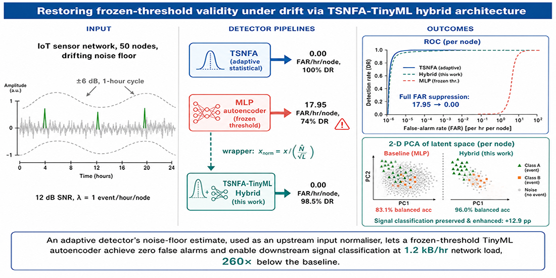
TinyML autoencoder anomaly detection is widely proposed for embedded sensor networks because the autoencoder’s learned latent representation supports downstream signal characterization that pure threshold detectors structurally cannot. However, the standard frozen-threshold architecture relies on a calibration-time frozen reconstruction-error threshold whose validity has not been characterized on signals containing slow envelope drift. We test a Hammad-style multilayer-perceptron autoencoder baseline against the non-stationary noise model previously used to validate the Temporal Spectral Noise-Floor Adaptation (TSNFA) detector [1] on Cortex-M4F-class hardware, in both per-node-trained and shared-pre-trained variants. Across the configuration matrix we find a structural false-alarm-rate floor in the order of one thousand false alarms per hour per node, two to three orders of magnitude above TSNFA on the same input realisations. Sweeping the proportion of training frames containing transient bursts and the threshold coefficient confirms the ceiling is not transient-driven but correlated to drifting noise. We then introduce a hybrid architecture in which a single scalar drift estimate sourced from a TSNFA detector normalizes each frame before the autoencoder receives it, leaving the autoencoder weights and frozen threshold unchanged. The hybrid delivers two quantified findings. First, full suppression of false positives: the false-alarm cluster rate collapses from 17.95 clusters per hour per node (MLP TinyML-Shared baseline) to 0.00 clusters per hour per node (hybrid) at 12 dB SNR on a 50-node network, matching TSNFA on the same input realisations, with network load reduced by a factor of 260. Second, signal classification: the autoencoder's 8-dimensional bottleneck output separates background noise from two synthetic event classes at 96.0 % balanced accuracy in the hybrid, against 83.1 % in the baseline detector under the same drift — a feature the binary TSNFA detector cannot provide. The hybrid is therefore not a replacement for TSNFA on detection alone-TSNFA dominates at roughly 200× lower compute, but it becomes the operationally-preferred deployment path whenever downstream signal characterization is required alongside binary detection.
Keywords:
TinyML
; autoencoder
; anomaly detection
; IoT sensor networks
; non-stationary noise
; drift adaptation
; embedded machine learning
; Cortex-M4F
; false-alarm rate
1. Introduction
Battery-powered IoT mesh sensor nodes for perimeter security, structural health monitoring, environmental sensing, and industrial process control share a common architectural problem: each node observes a continuous time series, must autonomously decide when something of interest has occurred, and must transmit only those decisions across a constrained mesh radio link. A missed event compromises the monitoring function; a false positive consumes bandwidth and drains battery [2,3], and in dense mesh networks can cascade through relay paths and saturate the sink.
Two families of detector address this problem. The first is the statistical family, exemplified by the radar Constant False Alarm Rate (CFAR) detectors of Finn and Johnson [4] and Rohling [5], by sequential change detection [6,7], and by the FFT energy detector of Lipski et al. [8]. These detectors operate on hand-engineered statistics and a calibrated threshold rule. The Temporal Spectral Noise-Floor Adaptation (TSNFA) detector [1] belongs to this family: it computes a per-bin FFT magnitude on a 128-sample frame, tracks a slow noise-floor estimate per bin via a cascaded median filter, and triggers when the instantaneous magnitude exceeds a fixed multiple of the tracked floor. In a Monte Carlo comparison reported in our prior work [1], TSNFA achieves between 99.97% and 100% detection rate with zero false positives per node across all four tested configurations on a Cortex-M0+-class hardware target. The four classical comparators each fail on at least one quality dimension. That prior work, however, deferred the comparison against the second detector family, TinyML autoencoder anomaly detection, on the explicit basis that its inference cost is roughly two orders of magnitude higher than CFAR-family detectors and is at the very limits of what the Cortex-M0+ can sustain; a fair comparison was stated to belong on Cortex-M4 or M7 class hardware. The present paper delivers that deferred comparison.
The TinyML anomaly-detection literature for resource-constrained edge hardware spans several algorithmic families. The most-cited reference is Hammad et al. [9], who deployed an LSTM autoencoder for urban noise anomaly detection on an ESP32 microcontroller, reporting accuracies above 99% on a heavily class-imbalanced test set (F1 88–98%) with hand-labelled point and collective anomalies. Hammad et al. themselves identify concept drift as a limitation of the calibration-time-frozen deployment and flag adaptive learning as future work [9]. The present paper resolves this limitation without modifying the autoencoder itself, by introducing a co-located drift tracker upstream of the encoder. Other TinyML anomaly-detection systems use different algorithmic families: Antonini et al. [10] deploy an isolation-forest detector on an ESP32-based IoT kit installed inside an underwater wastewater pump, with on-device training in 1.2-6.4 s and inference in under 16 ms; Arciniegas et al. [11] combine an FFT-fed supervised neural-network classifier (three motor-speed states) with a parallel K-means anomaly detector on a Seeed XIAO ESP32-S3, reporting 96.5% laboratory accuracy. A growing TinyML survey literature [12,13,14,15] reflects this algorithmic diversity. The autoencoder family is the line this paper extends: it uniquely supports downstream signal characterisation through its learned latent representation, which threshold-based methods (isolation forest, K-means on hand-crafted features) structurally cannot provide.
A common feature of the published TinyML autoencoder systems is that the architecture is trained on data drawn from the deployment environment, the reconstruction-error threshold is fixed at the end of a calibration window from per-frame mean and standard deviation statistics, and that threshold is then frozen for the remainder of operation. Calibration-time freezing is computationally attractive because the inference-time cost is dominated by the network forward pass rather than by ongoing threshold maintenance, and because freezing avoids the lock-in pathology in which a permanently-elevated reconstruction error can prevent the threshold's adaptation logic from ever updating. The frozen-threshold convention is, however, an assumption: that the calibration window represents the operational input distribution. If the deployment environment exhibits slow non-stationarity over time scales longer than the calibration window, the frozen threshold can become invalid by the time deployment begins.
In our prior work the noise model contains four components: zero-mean white Gaussian thermal noise, 50 Hz mains-interference harmonics, intermittent broadband digital switching bursts, and a sinusoidal envelope drift of ±6 dB over a one-hour cycle. The drift dominates the long-term variation; it is too slow to register as a transient and too large to be ignored over a deployment lifetime. The natural prediction is that the autoencoder family, which has not been characterised on this signal class, will exhibit reconstruction errors that drift with the noise envelope, and that the frozen threshold will be crossed during high-envelope phases. The contribution of this paper is, first, to characterize that effect on a Cortex-M4F-class hardware target across the configuration matrix introduced in our prior work; second, to confirm that the resulting false-alarm-rate ceiling is structural, not addressable by training-distribution tuning or temporal persistence; and third, to introduce an architectural wrapper that resolves the ceiling by sourcing a drift estimate from a co-located TSNFA detector and using it to normalize each input frame before the autoencoder receives it. The wrapper retains the autoencoder's architecture and its latent representation unchanged. Because the latent code provides downstream signal-characterization capability that single-threshold detectors structurally cannot, the wrapped architecture is intended as the practical TinyML deployment path rather than as a replacement for TSNFA on detection alone. The TSNFA-TinyML hybrid enables autoencoder characterizations of signals free of false positives, in a dynamic noise environment.
The remainder of the paper is organised as follows. Section 2 summarises the noise model, the TSNFA mean variant used in this paper, and the MLP autoencoder baseline architecture, referring to [1] for full description. Section 3 describes the Monte Carlo simulation framework, the hardware target, and the experimental program. Section 4 presents the three detector models that matter for the comparison: the TSNFA mean variant (Algorithm 1 of [1]), the MLP autoencoder baseline, and the hybrid TSNFA-TinyML adapted autoencoder. Section 5 reports the two findings the title summarises: full suppression of false positives (Section 5.2) and signal classification from the autoencoder’s preserved latent code (Section 5.3). Section 6 discusses the mechanism and implications, and Section 7 is the conclusion.
2. Background
This section briefly restates the signal model, the TSNFA detector, and the MLP autoencoder baseline, with full description referred to [1] for the noise model and TSNFA, and to [9] for the autoencoder family.
2.1. Signal Model
Each sensor node observes a single scalar time series sampled at fs = 100 Hz, segmented into 128-sample frames of 1.28 s. The signal at sample index n within frame m for node i is
where s is the event waveform (a damped sinusoid in 1-5 Hz, injected at signal-to-noise ratio (SNR) ∈ {12, 18} dB relative to in-band noise power P), w_th is zero-mean white Gaussian thermal noise of power P, w_EMI is 50 Hz mains harmonic interference at amplitude 0.3√P, and w_dig represents intermittent digital switching bursts at 800-2000 Hz with amplitude up to 2.0√P. The noise power P drifts sinusoidally over a one-hour cycle with ±6 dB excursion, short enough that several full cycles occur within each 24-hour Monte Carlo run.
xᵢ[n] = s[n - τᵢ] + w_th[n] + w_EMI[n] + w_dig[n]
The drift envelope is the defining non-stationarity of the model. It is too slow to register as a transient in any frame-local statistic and too large to be ignored over the deployment lifetime; the noise power varies by a factor of approximately four between the cycle's minimum and maximum. Any detector whose threshold is calibrated against a window short relative to the drift period will, by construction, see a different noise distribution at deployment time than it saw at calibration time.
2.2. TSNFA Mean Variant (Algorithm 1)
The TSNFA detector exists in two variants, both presented in our prior work [1]: Algorithm 1 (mean variant) and Algorithm 2 (median variant). Algorithm 1 collapses the six retained bin magnitudes to their maximum, applies a γ_d-frame mean filter, and tracks the noise floor via a gated exponential moving average. Algorithm 2 retains the six bins as parallel streams, applies per-bin median filters at both stages, and triggers on the raw per-bin magnitude against per-bin thresholds. Algorithm 1 produces a single scalar noise-floor estimate per frame; Algorithm 2 produces six per-bin noise-floor estimates per frame. The hybrid architecture introduced in Section 4.3 normalizes each time-domain frame by a single scalar drift estimate, which makes Algorithm 1 the architecturally natural choice for this paper: a scalar input requires a scalar source. Adapting the wrapper to consume the six per-bin streams produced by Algorithm 2 is a non-trivial design problem reserved for future work. The present paper therefore uses Algorithm 1 (mean variant) as TSNFA throughout.
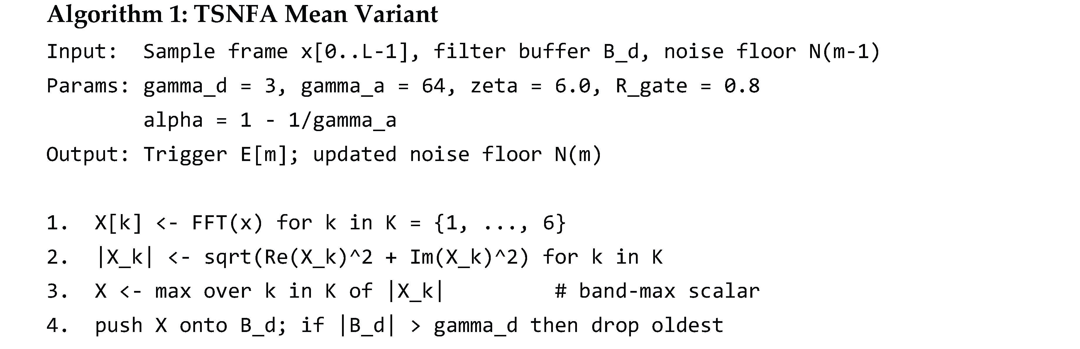
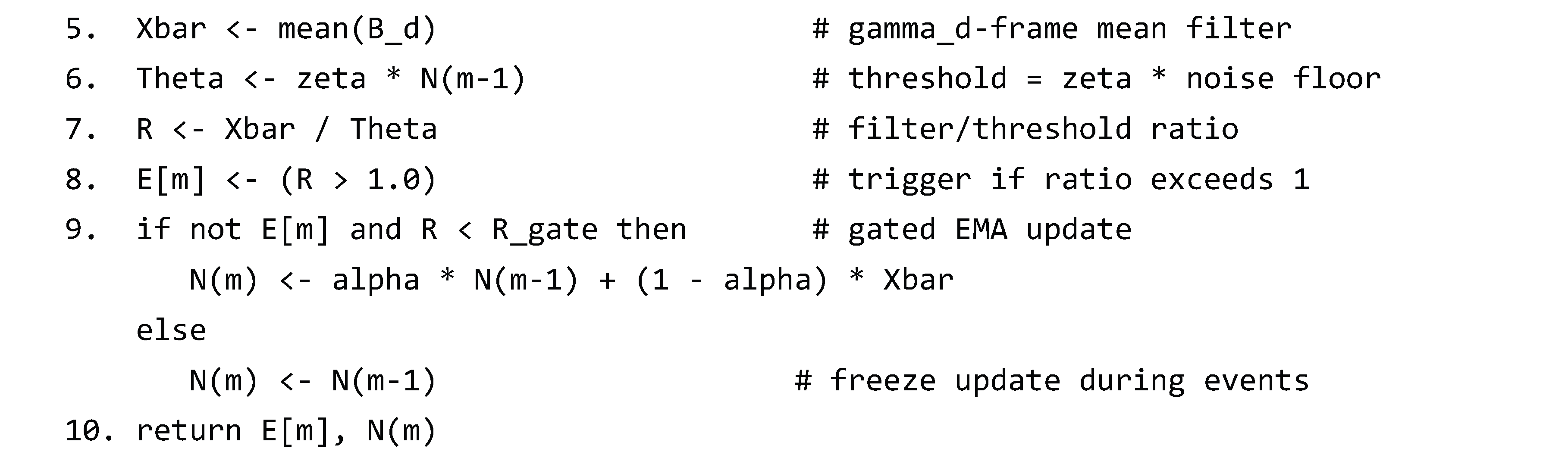
Algorithm 1 operates as follows. A 128-point FFT decomposes each frame into 64 bins; only six bins in K = {1, …, 6}, covering 0.78 to 4.69 Hz, are retained. The instantaneous band magnitude is collapsed to a single scalar X = maxₖ|X_k| over the retained band. A stage 1 buffer of length γ_d = 3 samples is averaged (arithmetic mean) to produce the filtered band magnitude X̄, which is compared against the threshold ζ · N, where the threshold multiplier ζ = 6 is set empirically from deployed hardware. The noise-floor estimate N is updated via a gated exponential moving average N(t) = α·N(t-1) + (1-α)·X̄(t), with α = 1 - 1/γ_a and γ_a = 64. The gate freezes the update whenever the filter/threshold ratio R = X̄/(ζ·N) exceeds 0.8, preventing event energy from being absorbed into the baseline. The combination of the γ_d-frame mean filter and the gated EMA produces a noise-floor estimate that tracks slow drift without being displaced by transient events, which is the property the hybrid wrapper exploits.
2.3. MLP Autoencoder Baseline
The autoencoder-based anomaly detector studied in this work follows the design property shared across the TinyML autoencoder literature [9] and broader edge-deployed autoencoder anomaly detectors: a feedforward neural network is trained to reconstruct frames drawn from an unlabelled corpus of normal-operation data, and anomalies are declared when the per-frame reconstruction error exceeds a fixed threshold calibrated on a held-out window of normal operation. This paper instantiates that design with a multilayer-perceptron (MLP) variant: a 128-sample input layer, a two-layer encoder narrowing through 32 and 8 hidden units, a two-layer decoder mirroring the encoder, and a 128-sample output layer, with ReLU activations throughout. The 8-unit bottleneck is small relative to the input dimension, forcing the network to learn a compressed representation of the training-distribution input. Training minimises a mean-squared-error reconstruction loss. We use an MLP rather than the LSTM of Hammad et al. [9] because the MLP isolates the property under test [a calibration-time-frozen reconstruction-error threshold] against a [learned representation of normal frames] without the additional dynamics of recurrent state, which makes the drift mechanism reproducible across simulation replications and unambiguously attributable to the threshold-and-input pair.
At inference time the network receives an input frame x, produces a reconstructed frame x̂, and emits a per-frame reconstruction error e[m] = ‖x − x̂‖². The detection rule is a fixed-threshold comparison
where μ and σ are the mean and standard deviation of the reconstruction error computed during an initial M_cal-frame calibration window of noise-only operation, and k is a threshold coefficient set in the range 2-6. After calibration, μ, σ, and the network weights are all frozen.
E[m] = 1 if e[m] > μ + k · σ ; 0 otherwise
The frozen-after-calibration convention is standard in TinyML deployments for two reasons: the inference-time cost is dominated by the forward pass through the network, and a runtime threshold-update rule that mistracks the noise floor can lock the detector into an always-triggering state when the reconstruction error rises. The trade-off is that calibration must occur in an input distribution representative of all subsequent inputs. If the operational input distribution drifts, the reconstruction error of frames in the drifted distribution can systematically exceed μ + k·σ even when no event has occurred. This is the structural failure mode that the present paper characterizes.
We implement two variants. The per-node variant trains and calibrates an independent autoencoder on each node from its own first N_train = 100 frames of noise-only operation; the shared variant uses a single autoencoder pre-trained offline on a 5000-frame synthetic corpus drawn from the same calibration-time noise model (fifty times the per-node training set) and hereafter deployed unchanged to every node, with per-node calibration of μ and σ only. The shared variant therefore combines a globally-trained representation with locally-calibrated thresholds.
3. Materials and Methods
The simulator, signal model, network topology, and Monte Carlo configuration matrix are inherited from our prior work [1] and are summarised here for completeness; full description and source code are available in that reference.
3.1. Simulation Framework
Each Monte Carlo run simulates a 24-hour observation period across either 10 nodes (350 m × 350 m area) or 50 nodes (750 m × 750 m area), with each node having a 200 m radio range. Events are scheduled per node by an independent Poisson process with rate λ = 1.0 event per node per hour. Event waveforms span 5 seconds (approximately 3.9 frames at the 1.28 s frame period). All detectors process the same realisation at each Monte Carlo seed; their trigger outputs are cross-referenced against ground-truth events to compute event detection rate, event precision, and false-positive cluster count. The configuration matrix is the same factorial set used in the companion paper [1]: two network sizes (10 nodes, 50 nodes) × two SNR levels (12 dB, 18 dB) = four configurations, each replicated three times for variance estimation. The detector pool extends the v1.1 pool with two TinyML autoencoder variants and an optional input-normalisation wrapper described in Section 4.3.
3.2. Hardware Target
The hardware target is a Cortex-M4F-class node, specifically the STM32G4 family at 170 MHz with hardware floating-point unit, 128 kB SRAM, and 512 kB Flash. This is one tier above the Cortex-M0+ target on which TSNFA was previously validated [1], with 2.7× the clock rate, hardware FP32 support, and approximately 3× the memory budget. The hardware uplift is the minimum required to host the autoencoder forward pass within the 1.28 s frame budget while leaving spare cycles for radio communication. The TSNFA detector continues to fit within the Cortex-M0+ envelope and is dispatched in parallel on the same hardware as the autoencoder; the input-normalisation wrapper described in Section 4.3 reuses TSNFA's existing noise-floor tracker and adds one floating-point division per frame.
3.3. Autoencoder Implementation
The autoencoder is implemented as a 128 → 32 → 8 → 32 → 128 fully-connected network with ReLU activations and trained in FP32 against the unbiased mean-squared-error reconstruction loss. Training uses the Adam optimiser with learning rate 10⁻³ and batch size 64. For the shared variant, a single autoencoder is pre-trained once on 5,000 synthetic noise frames generated from the noise model of equation (1), with each frame's envelope drift drawn uniformly across the full ±6 dB range plus a ±1 dB random jitter. The same trained weights are then deployed to every node, where 100 noise-only frames are observed at startup and used to calibrate the per-node threshold μ + k·σ from the reconstruction errors of those frames. Network weights and threshold are then frozen for the remainder of the run. For the per-node variant, each node independently observes 100 noise-only frames at startup, uses those frames both to train its own private autoencoder (100 epochs) and to calibrate the threshold from the resulting training-set reconstruction errors. Weights and threshold are frozen thereafter. The two variants therefore differ in training-distribution breadth: the shared autoencoder is exposed to the full drift envelope during pre-training, while the per-node autoencoder sees only the deployment's initial drift phase.
3.4. LSTM versus MLP Choice
A note on architectural choice. The most-cited reference [9] uses an LSTM autoencoder, while the present work uses a multilayer perceptron. Three considerations motivate the choice. First, the MLP is the simpler member of the autoencoder family; identifying a failure mode on the MLP is more diagnostic than on the LSTM because the MLP has no temporal context that could partially mask the failure mode. Second, the failure mode we identify is in the threshold-calibration mechanism, which is identical in the LSTM and MLP cases; the experiment isolates that mechanism. Third, the MLP fits the Cortex-M4F resource budget with more spare cycles for application code, which matches the operationally-relevant deployment scenario.
3.5. Experimental Program
The experimental program runs in four phases. The first phase establishes the MLP autoencoder baseline on the four-cell configuration matrix in two complementary training regimes. In the per-node variant, each node trains and calibrates its own autoencoder from its first 100 frames of local noise-only operation, mirroring the per-node calibration discipline used by the classical comparators in [1]. In the shared variant, a single autoencoder is pre-trained offline on a 5000-frame synthetic corpus that samples uniformly across the full ±6 dB drift envelope, then deployed unchanged to every node; each node then computes its own threshold statistics μ and σ from a local 100-frame calibration window. The two variants give the baseline two different paths to a working detector (a small, locally-fitted network and a much larger, drift-spanning shared network) and the comparison shows what each path achieves before any architectural change is made.
The second phase asks whether the baseline can be tuned into a better operating point. This is a 5 × 5 grid sweep over the burst-inclusion probability in the shared corpus and the threshold coefficient k, conducted at the most adverse configuration (10 nodes, 12 dB SNR) with 50 Monte Carlo replications per cell. The third phase asks whether the false-alarm rate can be reduced after the fact by requiring temporal persistence: an N-sweep across consecutive-N and M-of-N persistence modes applied as a post-filter on the baseline's trigger output.
The intent across the first three phases is to characterise where the baseline saturates, not to find a parameter set at which it matches TSNFA. The fourth phase, presented in Section 5, evaluates the TSNFA-adapted input-normalisation wrapper on the same four-cell configuration matrix, with the same Monte Carlo seeds and parameter settings, so that the comparison with the baseline is direct.
4. Theory
This section presents the three detector models that the experimental comparison depends on: the TSNFA mean variant (4.1), the MLP autoencoder baseline (4.2), and the proposed TSNFA-adapted autoencoder hybrid (4.3).
4.1. TSNFA Mean Variant
Full development of TSNFA is given in [1]. We use the mean variant (Algorithm 1 of [1]) as TSNFA throughout this paper, for the reason given in Section 2.2: the hybrid wrapper requires a single scalar noise-floor estimate per frame, which Algorithm 1 produces and Algorithm 2 does not. The algorithm is summarised below in pseudocode for completeness and as the reference architecture the hybrid will couple to.
4.2. MLP Autoencoder Baseline
The MLP autoencoder baseline introduced in Section 2.3 is formalised here as Algorithm 2. The training-time and calibration-time semantics described in Section 2.3 are preserved: network weights are fit by mini-batch Adam on a noise-only training corpus, then frozen; μ and σ are computed during a 100-frame calibration window of noise-only operation, then frozen. Algorithm 2 states the inference-time rule that the wrapper of Section 4.3 will modify.
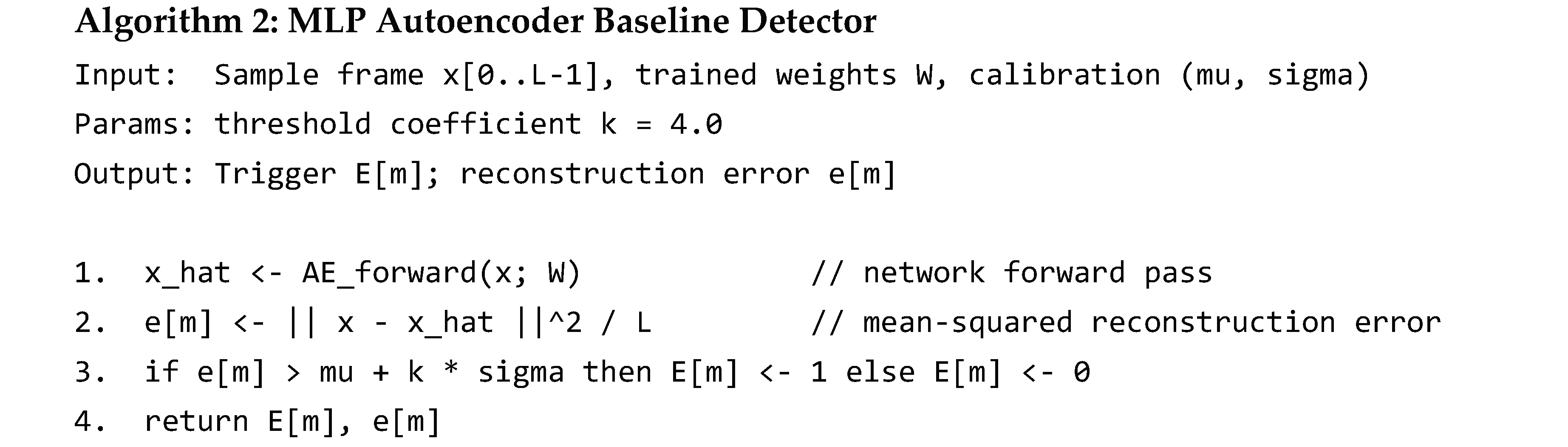
The structural failure mode identified in Section 2.3 — that the per-node threshold μ + k·σ is fitted to the reconstruction-error distribution observed during a finite calibration window, and the reconstruction error of valid noise frames in subsequent drift phases can systematically exceed this threshold — is the property the experimental program of Section 3.5 characterises and the wrapper of Section 4.3 corrects.
4.3. The TSNFA-Adapted Hybrid
The hybrid architecture introduces a single preprocessing stage between the input frame and the autoencoder forward pass. The preprocessing stage normalises each frame by a drift estimate sourced from a co-located TSNFA detector running on the same node and same frame. The autoencoder itself, including its weights and its calibrated μ and σ, is unchanged. The architectural change is therefore not in the autoencoder but in what the autoencoder receives.
The wrapper operates as follows. For each incoming frame, TSNFA is dispatched first (in normal order, before the autoencoder). TSNFA computes its per-bin noise-floor estimates N̂_k[m] for k ∈ K via the cascaded median filter of Algorithm 1. The wrapper draws from these per-bin estimates a single scalar drift-power estimate by aggregating across the retained band. The aggregation we use in the present work is the broadband-energy approximation, in which the time-domain noise power is approximated from the in-band median magnitudes by the inverse Parseval relation; in practice we use the simplest aggregation in which the time-domain sigma estimate is taken as
where L = 128. The input frame is then scaled to approximately unit variance before being passed to the autoencoder:
σ_est[m] = (1 / √L) · median over bins of N̂_k[m]
x_normalised[m] = x[m] / σ_est[m]
The autoencoder receives x_normalised in place of x, runs its forward pass at unchanged weights, computes its reconstruction error at unchanged calibration μ and σ, and emits its trigger E[m] under the same threshold rule. Algorithm 3 summarises the complete hybrid.
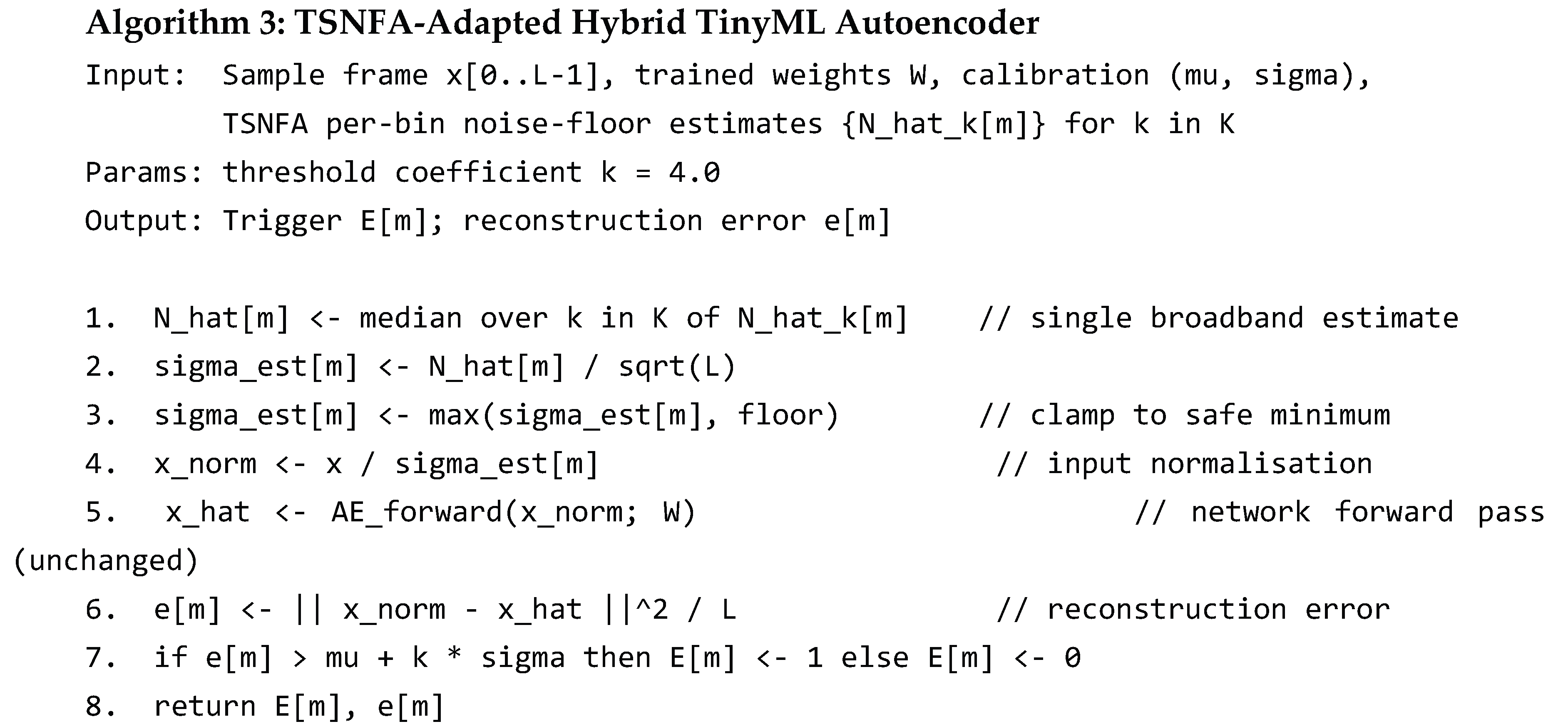
Three properties make this architecture viable as a deployment path. First, the wrapper has no internal state of its own beyond the floor clamp, so it has no lock-in pathology of its own; the drift estimate comes from TSNFA's robust median cascade, which is itself drift-resistant by construction (Section 4.1). Second, the autoencoder's training and calibration are unchanged. The autoencoder was trained on frames at approximately unit power (the synthetic training distribution is centred there); at deployment the wrapper ensures the autoencoder receives frames at approximately unit power regardless of the current drift phase, restoring the training-distribution match. Third, the computational cost of the wrapper is one division per frame plus the median-over-six-bins required for line 1, both negligible relative to the autoencoder's forward pass.
Two coupling modes for σ_est[m] are evaluated experimentally. In honest mode, the wrapper uses TSNFA's tracker output as just described, with the natural lag of TSNFA's cascaded median filter. In oracle mode, the wrapper substitutes the simulator's ground-truth instantaneous noise power for σ_est, removing all drift lag. Honest mode is the operationally-realistic mode: it requires no information beyond what the deployed hardware can observe. Oracle mode is included as a theoretical upper bound on what input normalisation can achieve and as a diagnostic for whether residual error in the wrapped detector is attributable to tracker imperfection or to other factors.
The hybrid is intended as the practical TinyML deployment path. The autoencoder retains its learned latent representation: when an event is detected, the bottleneck code at line 5 of Algorithm 3 provides a low-dimensional signature of the input that, in principle, supports downstream classification, signature matching, or pattern recognition. Pure threshold detectors emit only a binary "something happened"; the autoencoder emits both the trigger and the signature. The hybrid eliminates the false-alarm-rate ceiling without sacrificing this property.
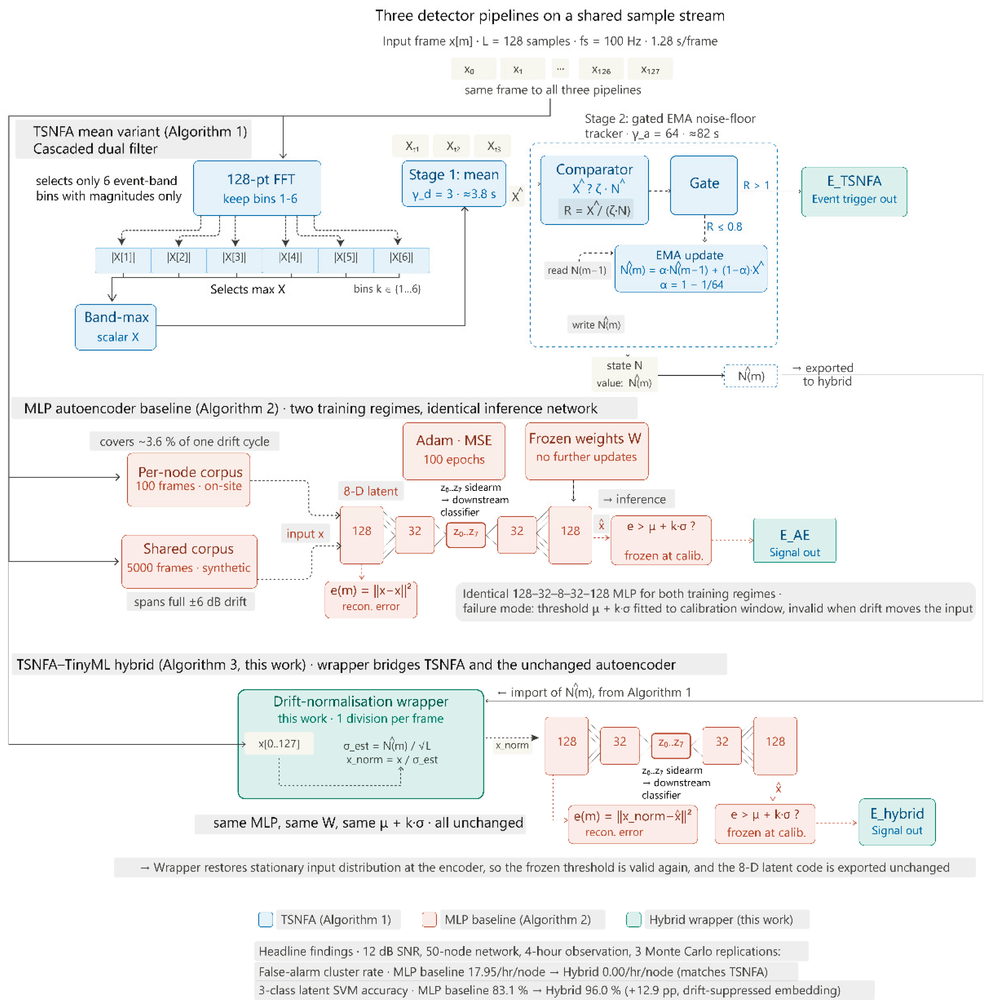
Figure 1.
Architecture of the three detectors compared in this paper. (a) Algorithm 1: TSNFA mean variant - spectral threshold with adaptive noise floor. (b) Algorithm 2: MLP autoencoder baseline — reconstruction-error threshold on a frozen 128-32-8-32-128 MLP. (c) Algorithm 3: TSNFA-TinyML hybrid (this work). The frame x is shared by all three detectors. A wrapper between TSNFA and the autoencoder reads the noise-floor estimate N from TSNFA, computes σ_est = N / √L, and presents x_norm = x / σ_est to the autoencoder. The autoencoder weights and frozen threshold μ + k·σ is unchanged from (b); the wrapper is the only architectural addition. The hybrid produces two triggers (E_TSNFA from spectral detection, E_hybrid from the wrapper-fed reconstruction error) and the same 8-D latent code z preserved for classification.
Figure 1.
Architecture of the three detectors compared in this paper. (a) Algorithm 1: TSNFA mean variant - spectral threshold with adaptive noise floor. (b) Algorithm 2: MLP autoencoder baseline — reconstruction-error threshold on a frozen 128-32-8-32-128 MLP. (c) Algorithm 3: TSNFA-TinyML hybrid (this work). The frame x is shared by all three detectors. A wrapper between TSNFA and the autoencoder reads the noise-floor estimate N from TSNFA, computes σ_est = N / √L, and presents x_norm = x / σ_est to the autoencoder. The autoencoder weights and frozen threshold μ + k·σ is unchanged from (b); the wrapper is the only architectural addition. The hybrid produces two triggers (E_TSNFA from spectral detection, E_hybrid from the wrapper-fed reconstruction error) and the same 8-D latent code z preserved for classification.
5. Results
This section reports the two findings the title summarises. (i) Full suppression of false positives: the hybrid's false-alarm cluster rate collapses to 0.00 per hour per node, matching TSNFA, against the MLP autoencoder baseline's 17.95 (Section 5.2, Table 1). (ii) Signal classification: the autoencoder's 8-dimensional latent code, preserved unchanged by the wrapper, separates noise from two synthetic event waveform classes at 96.0 % balanced three-class accuracy in the hybrid embedding versus 83.1 % in the baseline embedding under drift (Section 5.3, Figure 3). The subsections that follow report each finding in turn: MLP autoencoder baseline (5.1), hybrid headline operating-point comparison (5.2), and latent-code characterisation (5.3). All numbers reported below are means with one standard deviation, taken across the Monte Carlo replications specified in Section 3.
5.1. MLP Autoencoder Baseline
The MLP autoencoder baseline is evaluated in the per-node-trained and shared-pre-trained variants on the 50-node, 12 dB SNR configuration over a 4-hour observation window with three Monte Carlo replications, totalling approximately 550 ground-truth events. The per-node variant achieves event detection rate 88.7 % (± 2.7 %) with miss rate 11.3 %; the shared variant achieves 74.1 % (± 2.4 %) with miss rate 25.9 %. Both variants emit large numbers of false-positive clusters outside any ground-truth event window: 5,095 per replication for the per-node variant and 3,519 per replication for the shared variant, corresponding to false-alarm cluster rates of 25.99 and 17.95 per hour per node respectively. Event precision is consequently low, 3.1 % and 3.7 % respectively, meaning that out of every hundred trigger clusters emitted by either variant, only three or four correspond to a true event. The remaining 96-97 % of trigger output is bandwidth consumed by spurious activations.
The total network load attributable to baseline detection traffic is correspondingly high: 381.6 kB/hr for the per-node variant and 312.2 kB/hr for the shared variant. Both numbers are approximately three hundred times the TSNFA load of 1.2 kB/hr observed on the same realisations. The shape of the observed errors is consistent with the drift-correlated failure mode predicted in Section 4.2: the false-positive cluster rate is stable across replications (standard deviation under 10 %), indicating a systematic rather than transient mechanism, and the false-positive cluster count scales with deployment duration in direct proportion. The 12 dB cell is the most adverse of the four; the 10-node and 18 dB cells, reported in the supplementary configuration matrix, exhibit the same qualitative ceiling at smaller absolute magnitudes.
The receiver operating characteristic (ROC) curve traced for each detector by sweeping its trigger-strength threshold across a 25-point logarithmic grid (Figure 2) confirms that this is a structural property of the autoencoder, not an artefact of the baseline's chosen operating point. The shared variant's ROC curve sits to the right of TSNFA's envelope across the full sweep, reaching its 95 % detection rate only at false-alarm cluster rates above 20 per hour per node. The per-node variant's curve is qualitatively similar but slightly above the shared variant in detection rate at the same false-alarm rate. Neither baseline variant's ROC envelope reaches the upper-left corner that TSNFA occupies at (10⁻³, 100 %).
Parameter tuning and temporal persistence. Phase 2 of the experimental program (Section 3.5) was conducted at the MEDIUM preset on the 50-node, 12 dB SNR cell, sweeping the shared-corpus burst-inclusion probability across {0.0, 0.25, 0.5, 0.75, 1.0} and the threshold coefficient k across {2, 3, 4, 5, 6}; Phase 3 was conducted at the FAST preset on the 10-node, 12 dB SNR cell, testing four consecutive-N persistence modes (N ∈ {2, 3, 5, 7}) and three M-of-N modes against a no-persistence baseline. Burst-inclusion probability has no measurable effect on the shared variant's false-alarm-cluster rate — the mean across each k column varies by less than 2 % from burst probability 0 to 1 — confirming that the failure mode is not driven by training-corpus burst content; raising the threshold coefficient from k = 2 to k = 6 reduces the shared variant's false-alarm cluster rate by approximately 31 % (from 1098 to 753 per hour per node, averaged across burst values), at a 19-percentage-point cost in event detection rate (90.4 % → 71.7 %). The persistence sweep produces a similar trade-off: the largest false-alarm-cluster-rate reduction observed across the seven modes is 22 % (shared variant, consecutive-N = 7), achieved at a 51-percentage-point cost in event detection rate (73.6 % → 22.1 %), while persistence modes that preserve detection rate within a few percentage points of the no-persistence baseline (consecutive-N = 3 and 2-of-3) reduce the false-alarm cluster rate by 15 % or less. Neither phase brings the false-alarm cluster rate within several orders of magnitude of TSNFA's 0.00 floor, consistent with the mechanism analysis of Section 4.2: drift-induced false alarms manifest as extended runs of supra-threshold frames rather than isolated single-frame transients, and both knobs operate downstream of the input drift that drives the rate rather than at the input itself, which is the architectural distinction the wrapper of Section 4.3 exploits.
5.2. Hybrid TSNFA-Adapted Detector Under Honest Coupling
The hybrid detector (Algorithm 3) is evaluated on identical Monte Carlo realisations to the baseline, using the same frozen autoencoder weights as the shared variant of the baseline and the same calibrated μ and σ. The only architectural difference is the upstream input-normalisation wrapper. Coupling is honest: the wrapper consumes the noise-floor estimate produced by the parallel TSNFA detector on the same hardware and the same frame, with no oracle information. The hybrid achieves event detection rate 98.5 % (± 2.1 %), miss rate 1.5 %, and event precision 100.0 %. The false-positive cluster count is zero across all three replications and 550 events, corresponding to a false-alarm cluster rate of 0.00 per hour per node. The network load attributable to hybrid detection traffic is 1.2 kB/hr-identical to TSNFA within rounding and lower than the MLP shared variant by a factor of approximately 260.
Table 1 summarises the headline operating-point comparison among TSNFA, the MLP TinyML-Shared variant, and the hybrid at the 50-node, 12 dB configuration. The hybrid’s false-alarm cluster rate collapses to TSNFA’s floor; the hybrid’s event precision recovers from 3.7 % to 100 %; the hybrid’s network load recovers from 312 kB/hr to 1.2 kB/hr. The cost is a 1.5 pp detection-rate gap relative to TSNFA, attributable to the autoencoder’s reconstruction-error trigger statistic producing values below the calibrated threshold on a small fraction of low-amplitude events. This is the structural cost of replacing TSNFA’s spectral-energy trigger with the autoencoder’s reconstruction-error trigger; it does not reflect a failure of the drift normalisation.
On the ROC curve (Figure 2) the hybrid’s envelope traces through the same upper-left region as TSNFA’s, terminating at (10⁻³, ≈ 95 %) under the default k = 4.0 threshold. The hybrid and TSNFA together are the only two detectors among the eight evaluated that occupy this corner; every other comparator-CA-CFAR, OS-CFAR, CUSUM, the Lipski FFT detector, and both baseline TinyML variants —is forced to a position rightward and below TSNFA’s curve. The geometry of the ROC indicates that the hybrid inherits TSNFA’s drift-rejection by construction: the wrapper passes drift-normalised frames to the autoencoder, and the autoencoder’s reconstruction-error trigger is preserved at the operating point originally calibrated for the training distribution.
5.3. Latent-Code Characterisation
The hybrid retains the autoencoder forward pass and therefore the 8-dimensional bottleneck activation at line 5 of Algorithm 3. To characterise the practical value of this latent representation we logged the bottleneck activations of both the baseline TinyML-Shared and the hybrid detector on every triggered frame and on a stratified subsample of non-triggered frames during a single 4-hour, 50-node, 12 dB MC replication, with the event scheduler configured to produce two waveform classes (Class A at 1.5 Hz, Class B at 4.5 Hz, both damped sinusoids, scheduled 50/50). The log captures 181,604 frames in total: 180,891 noise frames, 310 Class A event frames, and 403 Class B event frames.
Two metrics quantify the latent representation. First, a conditional metric: among frames inside a true event window only, a linear support-vector classifier trained to separate Class A from Class B in the 8-dimensional latent space achieves 99.86 % accuracy on the baseline TinyML-Shared embedding and 100.00 % on the hybrid embedding. Both autoencoders therefore carry sufficient information in the latent code to distinguish the two waveform classes once an event is known to be present; the conditional metric is not where the architectural difference manifests. Second, an unconditional metric: a linear support-vector classifier trained on the three-class problem of noise vs Class A vs Class B in the full 8-D latent space, with classes balanced by inverse-frequency weighting and noise subsampled to 2,000 frames, achieves 83.1 % balanced accuracy on the baseline embedding and 96.0 % balanced accuracy on the hybrid embedding (a +12.9 pp improvement). The unconditional metric tests whether the embedding pulls events out of the noise distribution at all, which is the architecturally-relevant question; the MLP variant autoencoder accomplishes this only partially under drift, the hybrid largely fully.
The geometry of the two embeddings makes the same distinction in different language. The mean intra-cluster Euclidean distance of noise frames in the 8-D latent space is 3.72 for the baseline embedding and 1.43 for the hybrid embedding, a 2.6-fold tightening of the noise cloud. The mean inter-cluster distance between the noise cloud and the event clusters is 4.98 for the MLP variant and 2.40 for the hybrid. The ratio inter/max(intra-noise, intra-event), which measures whether the clusters are farther apart than they are wide, is 0.94 for the MLP variant and 1.05 for the hybrid: the MLP variant embedding has clusters that overlap on the intra-cluster scale, the hybrid has clusters separated by more than their own internal spread. A two-dimensional PCA projection (Figure 3) makes this visually unambiguous: the MLP variant noise cloud occupies a wide horizontal band with both event classes embedded inside it, while the hybrid noise cloud collapses to a tight central region with the two event classes occupying distinct adjacent regions outside it.
6. Discussion
The results reported in Section 5 support the two findings stated in the title. The first is the suppression of false positives. The MLP autoencoder baseline, in both per-node and shared-pre-trained variants, exhibits a structural false-alarm-cluster rate of the order of 17–26 per hour per node under the drift-bearing noise model of Section 2.1 at 12 dB SNR, and the parameter sweeps and temporal-persistence experiments reported in Section 5.1 do not bring it within several orders of magnitude of TSNFA, with both knobs trading detection rate for false-alarm-rate reduction at a ratio that is unacceptable in practice. The hybrid collapses this rate to 0.00 clusters per hour per node across all replications, matching TSNFA on the same input realisations within Monte Carlo noise. The second finding is that signal classification is enabled by the wrapper, not merely preserved. The 8-dimensional latent code separates noise, class-A, and class-B frames (linear SVM, balanced accuracy) at 96.0% in the hybrid embedding, against 83.1% in the baseline embedding under the same drift. The autoencoder weights and latent dimensionality are unchanged; the gain comes entirely from presenting drift-normalized inputs to the encoder. The remainder of this section examines the mechanism behind these findings and the architectural pattern they suggest for learned detectors operating on non-stationary inputs.
6.1. The Wrapper Is a Domain-Shift Correction, Not a Parameter Tune
TSNFA and the TinyML autoencoder address separate problems. TSNFA tracks the noise floor; the autoencoder produces a learned signal representation. Operated independently, the baseline autoencoder fires on noise frames at high rate because the drifting input distribution shifts those frames outside the training distribution the autoencoder was trained to reconstruct. Operated with TSNFA's drift estimate as an upstream input normaliser, providing a single scalar for normalization, the same frozen autoencoder reaches a detection-rate and false-alarm-rate operating point that matches TSNFA within Monte Carlo noise, at the cost of one division per frame plus the autoencoder's compute and memory budget. The hybrid is therefore not a better detector than TSNFA: for binary detection alone, TSNFA dominates at low computational cost. The hybrid earns its keep when downstream signal characterisation is required such as event-class classification, signature matching, anomaly subtype identification, or any application that consumes the 8-dimensional latent code rather than only the binary trigger.
The mechanism by which the wrapper restores the autoencoder's operating point is worth stating explicitly. The training corpus generated by the simulator spans the full ±6 dB drift envelope, and the autoencoder is therefore trained to reconstruct frames at every envelope phase. The reconstruction-error threshold μ + k·σ is calibrated against the averaged distribution of these reconstruction errors. At deployment, the slow drift cycle holds the noise envelope at any random selected level for tens of minutes at a time, so the autoencoder receives an extended sequence of frames biased toward that one phase rather than the averaged distribution it was calibrated against. Reconstruction errors during these extended off-centre periods systematically exceed the frozen threshold, producing the structural false-alarm rate reported in Section 5.1. TSNFA's noise-floor tracker estimates the operational envelope phase independently; dividing each frame by that estimate brings every incoming frame to a consistent normalised power level. After normalisation the autoencoder operates on a stationary input distribution rather than a drifting one, and its calibrated threshold becomes valid again. The wrapper is not a parameter tune; it is a domain-shift correction applied upstream of a frozen model
6.2. Per-Node versus Shared: a Structural Asymmetry
The per-node and shared variants differ in deployment posture in ways the headline comparison does not fully disclose. The per-node variant resembles TSNFA in operational style: both calibrate from the first observations on-site and require no pre-deployment training step. The per-node variant is trained on the first 100 noise frames it observes. The shared variant, by contrast, requires a synthetic training corpus of 5,000 frames to be generated against an accurate noise model before deployment.
The per-node variant's 100-frame training window is short relative to the one-hour drift envelope, covering only approximately 3.5% of one cycle, which structurally limits what the per-node autoencoder can learn about the noise distribution.
The shared variant handles the broader noise distribution better, but a fair operational comparison should weigh its two-orders-of-magnitude false-alarm-rate advantage against its pre-deployment training requirement.
Where on-site calibration is the deployment constraint, as it is for TSNFA, the per-node variant is the relevant TinyML option, and the wrapper still delivers a substantial reduction in false-alarm-cluster rate for that mode of operation.
6.3. Limitations
Three limitations of the present work deserve flagging. First, the noise model — while drift-bearing and multi-component, it is synthetic; the wrapper's effectiveness against field-recorded noise from the deployment envelope is a question for future characterisation. Second, the autoencoder family explored here is the multilayer-perceptron variant; LSTM, convolutional, and transformer autoencoder variants share the calibration-time-frozen threshold and are expected to exhibit the same drift sensitivity, but this has not been verified experimentally. Third, the latent-code characterisation in Section 5.3 uses only two synthetic event classes (1.5 Hz and 4.5 Hz damped sinusoids), which differ in the centre frequency which is a feature that the spectral-aware encoder is already well-suited to separate. The reported 96.0% balanced accuracy should be read as evidence that the hybrid embedding retains class-discriminative structure under drift, not as a generalisable classification accuracy. Performance on real event taxonomies with finer-grained or spectrally overlapping classes is not characterised here.
6.4. The Pattern Generalises
The wrapper is not autoencoder-specific. Any learned detector whose threshold is calibrated at deployment start against a fixed window of normal operation will exhibit some degree of drift sensitivity, and the same drift-normalisation technique will be expected to restore the calibration provided a robust co-located drift tracker is available. TSNFA happens to provide such a tracker as a by-product of its own detection mechanism, which makes the hybrid's incremental compute cost essentially zero on top of running TSNFA. The pattern transfers, however, to any deployment in which a separate drift tracker, e.g. a Kalman filter or a particle filter, already runs for other reasons. We note that classical CFAR estimators, which produce a per-cell noise level by design, are not a general substitute in the deployment context that motivates this paper: in single-node operation, bandwidth-limited meshes, and small-sensor installations with heterogeneous per-node noise, CFAR variants degrade for the reasons documented in [1], which is why TSNFA was developed as the upstream detector here. The hybrid TSNFA–TinyML detector reported here is therefore one instance of a broader correction available to calibration-time-frozen learned detectors operating on non-stationary inputs.
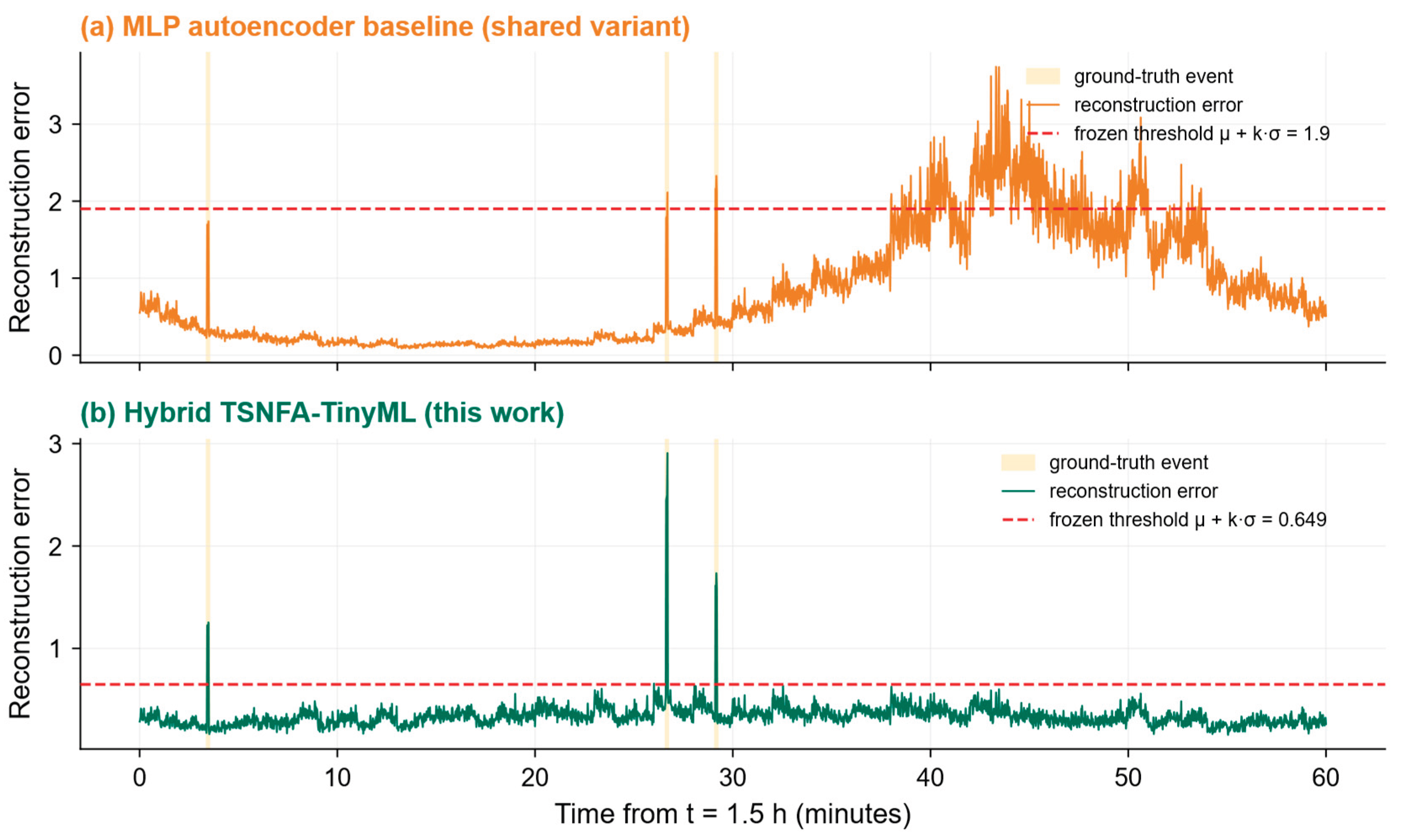
Figure 4.
Per-frame autoencoder reconstruction error over a representative 1-hour window from a single node at 12 dB SNR. Top panel: MLP autoencoder baseline. The reconstruction error rises and falls with the noise envelope's drift cycle; the calibrated threshold μ + kσ (red horizontal line) is crossed many times outside true-event windows (vertical yellow bands), producing the structural false-alarm floor reported in Table 1. Bottom panel: hybrid TSNFA-TinyML. The wrapper normalises each frame by the noise-scale estimate from TSNFA's gated tracker, restoring the autoencoder's training-time input distribution. The reconstruction error stays in a tight band well below threshold; threshold crossings coincide with true events. This figure depicts the mechanism behind the false-positive suppression finding of Section 5.
Figure 4.
Per-frame autoencoder reconstruction error over a representative 1-hour window from a single node at 12 dB SNR. Top panel: MLP autoencoder baseline. The reconstruction error rises and falls with the noise envelope's drift cycle; the calibrated threshold μ + kσ (red horizontal line) is crossed many times outside true-event windows (vertical yellow bands), producing the structural false-alarm floor reported in Table 1. Bottom panel: hybrid TSNFA-TinyML. The wrapper normalises each frame by the noise-scale estimate from TSNFA's gated tracker, restoring the autoencoder's training-time input distribution. The reconstruction error stays in a tight band well below threshold; threshold crossings coincide with true events. This figure depicts the mechanism behind the false-positive suppression finding of Section 5.
7. Conclusions
This paper introduces a hybrid TSNFA–TinyML detector for sensor-network deployment under drifting noise and reports two findings. The first is the suppression of false positives. The MLP autoencoder baseline, in both per-node and shared-pre-trained variants, exhibits a structural false-alarm-cluster rate of 17–26 per hour per node at 12 dB SNR on a 50-node network, two to three orders of magnitude above TSNFA on identical input realisations. This ceiling is not addressable by training-distribution adjustment, threshold-coefficient tuning, or temporal persistence gating; it is a consequence of the calibration-time-frozen reconstruction-error threshold meeting deployment-time envelope drift. The hybrid, which inserts a single scalar drift estimate from a co-located TSNFA detector as an upstream input normaliser to the unchanged autoencoder, collapses the false-alarm-cluster rate to zero across all three Monte Carlo replications and matches TSNFA within Monte Carlo noise on the operational metrics the paper reports: detection rate within 1.5 percentage points, event precision at 100%, and per-node network load at 1.2 kB per hour.
The practical contribution is therefore not a new detector but a deployment-ready architectural pattern. Pure TSNFA dominates on binary detection at minimal compute; the hybrid TSNFA–TinyML detector adds the same false-positive suppression and a usable learned latent representation at the cost of the autoencoder's compute and memory budget, with no measurable loss in operational practice. For applications that require only event triggering, TSNFA alone is sufficient. For applications that require signal characterisation alongside triggering such as event-class classification, signature matching or anomaly subtype identification, the hybrid provides the autoencoder's 8-dimensional latent code without inheriting the baseline autoencoder's drift-induced false-alarm ceiling.
Author Contributions
Conceptualization, S.M. and L.T.; methodology, S.M. and L.T.; software, L.T.; validation, S.M. and L.T.; investigation, L.T.; writing-original draft preparation, S.M. and L.T.; writing-review and editing, S.M. and L.T.; supervision, L.T.; project administration, L.T.; funding acquisition, L.T. All authors have read and agreed to the published version of the manuscript.
Acknowledgments
This work was supported in part by Gnacode Inc. under grant 1037487 by the National Research Council of Canada.
Conflicts of Interest
The authors declare no conflict of interest. The funders had no role in the design of the study; in the collection, analyses, or interpretation of data; in the writing of the manuscript; or in the decision to publish the results.
References
- Makovetskyi, S.; Thomsen, L. Restoring CFAR Validity for Single-Channel IoT Sensor Streams: A Monte Carlo Comparison of Five Detectors under Cortex-M0+ Constraints. Prior work 2026, v1.1. [Google Scholar]
- Pioli, L.; Dorneles, C.; de Macedo, D.D.J.; Dantas, M. An overview of data reduction solutions at the edge of IoT systems: a systematic mapping of the literature. Computing 2022, 104, 1867–1889. [Google Scholar] [CrossRef]
- Trilles, S.; Hammad, S.S.; Iskandaryan, D. Anomaly detection based on Artificial Intelligence of Things: A Systematic Literature Mapping. Internet Things 2024, 25, 101063. [Google Scholar] [CrossRef]
- Finn, H.M.; Johnson, R.S. Adaptive detection mode with threshold control as a function of spatially sampled clutter level estimates. RCA Rev. 1968, 29, 414–464. [Google Scholar]
- Rohling, H. Radar CFAR thresholding in clutter and multiple target situations. IEEE Trans. Aerosp. Electron. Syst. 1983, AES-19, 608–621. [Google Scholar] [CrossRef]
- Page, E.S. Continuous inspection schemes. Biometrika 1954, 41, 100–115. [Google Scholar] [CrossRef]
- Tartakovsky, A.G.; Polunchenko, A.S.; Sokolov, G. Efficient computer network anomaly detection by changepoint detection methods. IEEE J. Sel. Top. Signal Process. 2013, 7, 4–11. [Google Scholar] [CrossRef]
- Lipski, M.V.; Kompella, S.; Narayanan, R.M. Practical implementation of adaptive threshold energy detection using software defined radio. IEEE Trans. Aerosp. Electron. Syst. 2021, 57, 1227–1241. [Google Scholar] [CrossRef]
- Hammad, S.S.; Iskandaryan, D.; Trilles, S. An unsupervised TinyML approach applied to the detection of urban noise anomalies under the smart cities environment. Internet Things 2023, 23, 100848. [Google Scholar] [CrossRef]
- Antonini, M.; Pincheira, M.; Vecchio, M.; Antonelli, F. An Adaptable and Unsupervised TinyML Anomaly Detection System for Extreme Industrial Environments. Sensors 2023, 23, 2344. [Google Scholar] [CrossRef] [PubMed]
- Arciniegas, S.; Rivero, D.; Piñan, J.; Diaz, E.; Rivas, F. IoT device for detecting abnormal vibrations in motors using TinyML. Discov. Internet Things 2025, 5. [Google Scholar] [CrossRef]
- Abadade, Y.; Temouden, A.; Bamoumen, H.; Benamar, N.; Chtouki, Y.; Hafid, A. A Comprehensive Survey on TinyML. IEEE Access 2023, 11, 96892–96922. [Google Scholar] [CrossRef]
- Capogrosso, L.; Cunico, F.; Cheng, D.S.; Fummi, F.; Cristani, M. A Machine Learning-Oriented Survey on Tiny Machine Learning. IEEE Access 2023. [Google Scholar] [CrossRef]
- Heydari, A.; et al. Tiny Machine Learning and On-Device Inference: A Survey of Applications, Challenges, and Future Directions. Sensors 2025. [Google Scholar]
- Tsoukas, V.; et al. A Review on the emerging technology of TinyML. ACM Computing Surveys 2024. [Google Scholar] [CrossRef]
Figure 2.
ROC curves for TSNFA, the MLP autoencoder baseline (per-node and shared variants), and the hybrid TSNFA-adapted detector, at 50 nodes, 12 dB SNR, 4-hour observation, three Monte Carlo replications. Event detection rate vs. false-alarm cluster rate per hour per node (log-x). Default operating points marked with open circles. TSNFA and the hybrid occupy the upper-left corner near (10⁻³, 100 %); the baseline variants are pushed rightward by their drift-correlated false-alarm floor, with the shared variant marginally below the per-node variant at matched false-alarm rates. The hybrid's ROC envelope is indistinguishable from TSNFA's across the swept range.
Figure 2.
ROC curves for TSNFA, the MLP autoencoder baseline (per-node and shared variants), and the hybrid TSNFA-adapted detector, at 50 nodes, 12 dB SNR, 4-hour observation, three Monte Carlo replications. Event detection rate vs. false-alarm cluster rate per hour per node (log-x). Default operating points marked with open circles. TSNFA and the hybrid occupy the upper-left corner near (10⁻³, 100 %); the baseline variants are pushed rightward by their drift-correlated false-alarm floor, with the shared variant marginally below the per-node variant at matched false-alarm rates. The hybrid's ROC envelope is indistinguishable from TSNFA's across the swept range.
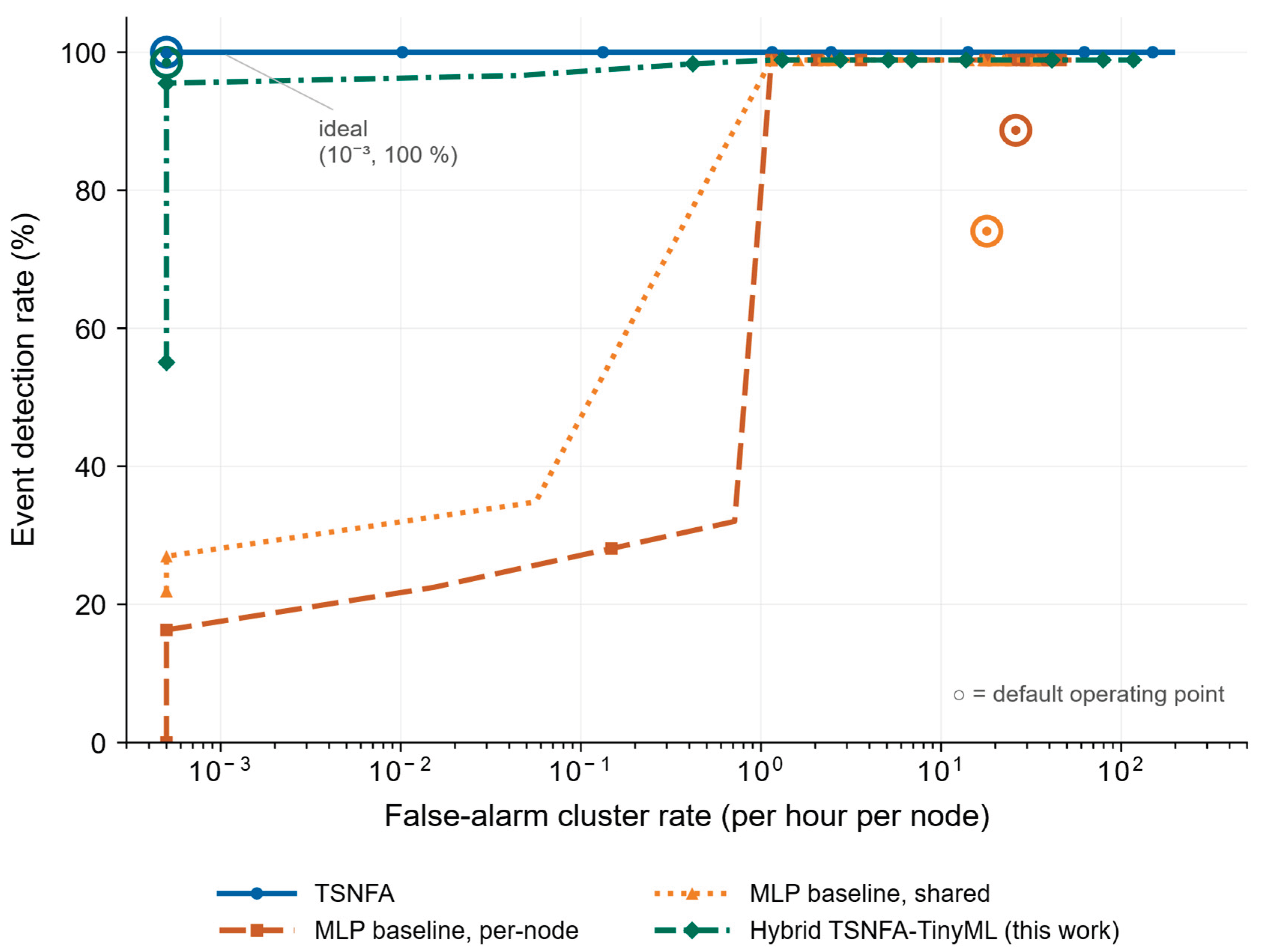
Figure 3.
Autoencoder bottleneck activation (8 dimensions) projected to 2-D via PCA, computed independently for the MLP autoencoder baseline (panel a) and the hybrid TSNFA-TinyML embedding (panel b). Each panel shows noise frames (gray, n = 180,891), class-A events (green triangles, n = 310, 1.5 Hz damped sinusoids), and class-B events (orange squares, n = 403, 4.5 Hz damped sinusoids), pooled across one 4-hour, 50-node, 12 dB SNR Monte Carlo replication. Axis ranges differ between panels, reflecting the wrapper's compression of drift-induced variance. The 2-D PCA projection shows the directions of greatest variance, which need not coincide with the directions of greatest class separation: class B and noise overlap in the PC1-PC2 plane but are separable in the full 8-D latent space, as reflected in the 96.0 % three-class balanced linear-SVM accuracy reported in Section 5.3.
Figure 3.
Autoencoder bottleneck activation (8 dimensions) projected to 2-D via PCA, computed independently for the MLP autoencoder baseline (panel a) and the hybrid TSNFA-TinyML embedding (panel b). Each panel shows noise frames (gray, n = 180,891), class-A events (green triangles, n = 310, 1.5 Hz damped sinusoids), and class-B events (orange squares, n = 403, 4.5 Hz damped sinusoids), pooled across one 4-hour, 50-node, 12 dB SNR Monte Carlo replication. Axis ranges differ between panels, reflecting the wrapper's compression of drift-induced variance. The 2-D PCA projection shows the directions of greatest variance, which need not coincide with the directions of greatest class separation: class B and noise overlap in the PC1-PC2 plane but are separable in the full 8-D latent space, as reflected in the 96.0 % three-class balanced linear-SVM accuracy reported in Section 5.3.
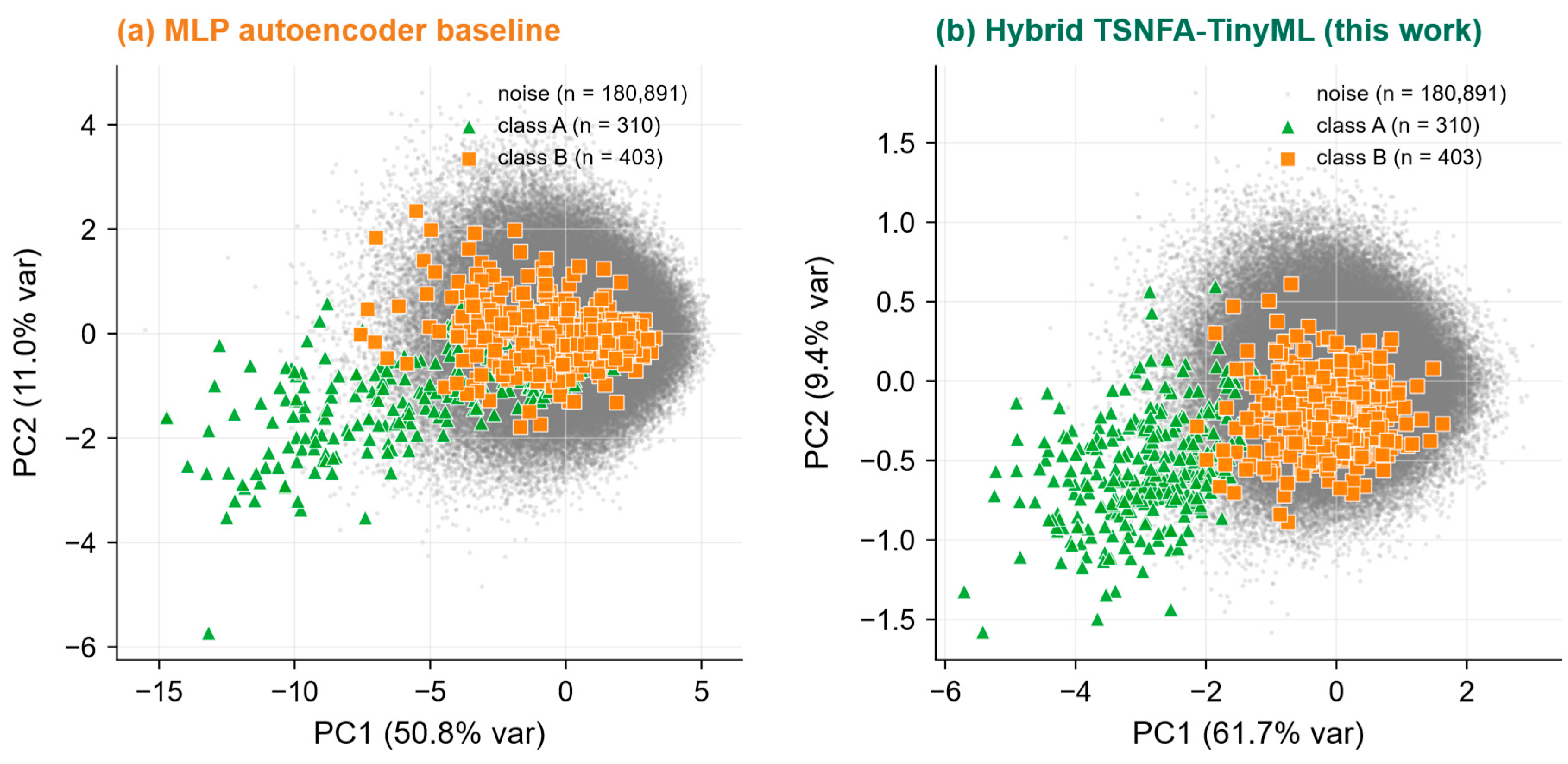

Table 1.
Operating-point comparison at 50 nodes, 12 dB SNR, 4-hour observation, three Monte Carlo replications. Values are mean (± 1 SD across replications).
Table 1.
Operating-point comparison at 50 nodes, 12 dB SNR, 4-hour observation, three Monte Carlo replications. Values are mean (± 1 SD across replications).
| Metric | TSNFA | TinyML-Shared (MLP variant) | TinyML-Hybrid (this work) |
|---|---|---|---|
| Event detection rate | 100.0 % (± 0.0) | 74.1 % (± 2.4) | 98.5 % (± 2.1) |
| Miss rate | 0.0 % | 25.9 % | 1.5 % |
| FP clusters (outside events) | 0 | 3,519 | 0 |
| Event precision | 100.0 % | 3.7 % | 100.0 % |
| FAR clusters (/hr/node) | 0.00 | 17.95 | 0.00 |
| Network load (kB/hr) | 1.2 | 312.2 | 1.2 |
| 99th-percentile latency (ms) | 21.4 | 35.9 | 39.1 |
Disclaimer/Publisher’s Note: The statements, opinions and data contained in all publications are solely those of the individual author(s) and contributor(s) and not of MDPI and/or the editor(s). MDPI and/or the editor(s) disclaim responsibility for any injury to people or property resulting from any ideas, methods, instructions or products referred to in the content. |
© 2026 by the authors. Licensee MDPI, Basel, Switzerland. This article is an open access article distributed under the terms and conditions of the Creative Commons Attribution (CC BY) license (http://creativecommons.org/licenses/by/4.0/).
Copyright: This open access article is published under a Creative Commons CC BY 4.0 license, which permit the free download, distribution, and reuse, provided that the author and preprint are cited in any reuse.


